Radiative corrections to the Casimir energy in the $\lambda|\phi|^{4}$ model under quasi-periodic boundary conditions

F. A. Barone

Centro Brasileiro de Pesquisas Físicas

Rua Dr. Xavier Sigaud, 150, Urca, 22290-180 Rio de Janeiro, RJ, Brazil

R. M. Cavalcanti and C. Farina

Instituto de Física, Universidade Federal do Rio de Janeiro

Caixa Postal 68528, 21941-972 Rio de Janeiro, RJ, Brazil

Abstract

We compute the first radiative correction to the Casimir energy in the $(d+1)$-dimensional $\lambda|\phi|^{4}$ model submitted to quasi-periodic boundary conditions in one spatial direction. Our results agree with the ones found in the literature for periodic and anti-periodic boundary conditions, special cases of the quasi-periodic boundary conditions.

The idea of introducing an arbitrary parameter in order to interpolate continuously distinct theories is not new in the literature. For instance, fermionic and bosonic partition functions can be obtained as particular cases of more general ones which are computed assuming that these fields satisfy a more general boundary conditions (BC) in the imaginary time, where the fields acquire a phase $e^{i\theta}$ whenever $\tau\rightarrow\tau+\beta$ ($\beta=1/T$) [1] (for non-relativistic partition functions see Ref. [2]). Periodic and antiperiodic BC (for bosons and fermions, respectively) correspond to $\theta=0$ and $\theta=\pi$.

It can be shown that the same effects can be obtained if instead of introducing the parameter $\theta$, we couple the charged field (bosonic or fermionic) appropriately with a constant gauge potential of the form $(A_{0},{\bf 0})$, which cannot be gauged away due to the compactification in the $x_{0}$-direction, introduced to take into account the thermal effects.

Similarly, we can consider that the field under study is submitted to quasi-periodic BC in a space dimension, which interpolates the periodic and antiperiodic ones. Analogously, the introduction of the interpolating parameter is equivalent to coupling the charged field with a constant gauge field with a non-vanishing component along the space-dimension which is assumed to be compactified [3].

In this work we discuss the effects of an interpolating BC in the vacuum energy of a complex scalar field. More precisely, we compute the $O(\lambda)$ correction to the Casimir energy of a complex scalar field whose dynamics is described by the (Euclidean) lagrangian density

$${\cal L}_{\rm E}=|\partial_{\mu}\phi|^{2}+m^{2}|\phi|^{2}+\lambda|\phi|^{4}+{\cal L}_{\rm ct},$$ (1)

where ${\cal L}_{\rm ct}$ contains the renormalization counterterms, and subject to quasi-periodic boundary conditions in the $x_{d}$-direction, i.e.,

$$\phi(x_{0},x_{1},\ldots,x_{d}+a)=e^{i\theta}\phi(x_{0},x_{1},\ldots,x_{d}),\qquad 0\leq\theta<2\pi.$$ (2)

In previous works we performed similar calculations for Dirichlet-Dirichlet, Neumann-Neumann [4], and Dirichlet-Neumann [5] boundary conditions.

The Casimir energy (per unit area) of a free field subject to those boundary conditions was computed in [6] in the $(3+1)$-dimensional case; the result is

$${\cal E}_{\theta}^{(0)}(a)\Big{|}_{d=3}=-\frac{m^{2}}{\pi^{2}a}\sum_{n=1}^{\infty}\frac{1}{n^{2}}\,\cos(n\theta)\,K_{2}(nma),$$ (3)

where $K_{\nu}(z)$ is the modified Bessel. In the massless limit Eq. (3) becomes

$${\cal E}_{\theta}^{(0)}(a)\Big{|}_{d=3,\,m=0}=-\frac{2}{\pi^{2}a^{3}}\sum_{n=1}^{\infty}\frac{\cos(n\theta)}{n^{4}}=\frac{2\pi^{2}}{3a^{3}}\,B_{4}\left(\frac{\theta}{2\pi}\right)\qquad(0\leq\theta<2\pi),$$ (4)

where $B_{4}(x)=x^{4}-2x^{3}+x^{2}-1/30$ is the Bernoulli polynomial of fourth degree [7] (see Fig. 1).

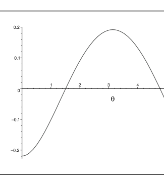
Figure 1: $a^{3}{\cal E}_{\theta}^{(0)}(a)$ as a function of $\theta$ for a massless field in ($3+1$) dimensions.

The $O(\lambda)$ correction to (3) is formally given by

$${\cal E}^{(1)}=\int_{0}^{a}dx_{d}\left[\lambda G^{2}(x,x)+\delta m^{2}\,G(x,x)+\delta\Lambda\right],$$ (5)

where $G(x,x^{\prime})$ is the Green’s function of the free theory (i.e., with $\lambda=0$, but obeying the boundary conditions), $\delta m^{2}$ is the radiatively induced shift in the mass parameter, and $\delta\Lambda$ is the shift in the cosmological constant (i.e., the change in the vacuum energy which is due solely to the interaction, and not to the confinement).

The spectral representation of $G(x,x^{\prime})$ in $d+1$ dimensions is given by

$$G(x,x^{\prime})=\frac{1}{a}\int{d^{d}k\over(2\pi)^{d}}\,e^{i{\bf k}\cdot({\bf x}-{\bf x}^{\prime})}\sum_{n=-\infty}^{\infty}\frac{e^{iq_{n}(z-z^{\prime})}}{{\bf k}^{2}+q_{n}^{2}+m^{2}}\ ,$$ (6)

where ${\bf x}=(x_{0},\ldots,x_{d-1})$, $z=x_{d}$, and $q_{n}=(2n\pi+\theta)/a$. $G(x,x^{\prime})$ diverges when $x^{\prime}\to x$ for $d\geq 1$, therefore a regularization prescription is needed in order that $G(x,x)$ makes sense. We shall compute it using dimensional regularization; the result is

$$G(x,x)={\Gamma\left(1-d/2\right)\over(4\pi)^{d/2}a}\sum_{n=-\infty}^{\infty}\omega_{n}^{d-2}\qquad(d<1),$$ (7)

where $\omega_{n}=\sqrt{q_{n}^{2}+m^{2}}$. Inserting this result into Eq. (5) and arranging terms, we obtain

$${\cal E}^{(1)}_{\theta}={\lambda\over a}\left[{\Gamma(1-d/2)\over(4\pi)^{d/2}}\sum_{n=-\infty}^{\infty}\omega_{n}^{d-2}+{a\,\delta m^{2}\over 2\lambda}\right]^{2}+a\left[\delta\Lambda-{(\delta m^{2})^{2}\over 4\lambda}\right].$$ (8)

In order to compute the sum that appears in Eq. (8) it is convenient to reexpress it as

$$\sum_{n=-\infty}^{\infty}\omega_{n}^{d-2}=\left({2\pi\over a}\right)^{d-2}{\cal D}\left({2-d\over 2},{ma\over 2\pi},{\theta\over 2\pi}\right),$$ (9)

where ${\cal D}$ is defined as

$${\cal D}\left(s,\nu,\frac{\theta}{2\pi}\right):=\sum_{n=-\infty}^{\infty}\left[\nu^{2}+\left(n+\frac{\theta}{2\pi}\right)^{2}\right]^{-s},\qquad{\rm Re}(s)>1/2.$$ (10)

The function ${\cal D}$ has an analytic continuation to the whole complex $s$-plane given by [2]

$${\cal D}\left(s,\nu,\frac{\theta}{2\pi}\right)=\frac{\sqrt{\pi}\,\nu^{1-2s}}{\Gamma(s)}\left[\Gamma\left(s-\frac{1}{2}\right)+4\sum_{n=1}^{\infty}\cos(n\theta)\,\frac{K_{1/2-s}(2n\pi\nu)}{(n\pi\nu)^{1/2-s}}\right],$$ (11)

with simple poles at $s=1/2,-1/2,-3/2,\ldots$ Inserting Eqs. (9) and (11) into Eq. (8) yields

$${\cal E}^{(1)}_{\theta} = {\lambda\over a}\left\{\frac{am^{d-1}}{(4\pi)^{(d+1)/2}}\left[\Gamma\left(\frac{1-d}{2}\right)+4\sum_{n=1}^{\infty}\cos(n\theta)\,\frac{K_{(d-1)/2}(nma)}{(nma/2)^{(d-1)/2}}\right]+{a\,\delta m^{2}\over 2\lambda}\right\}^{2}$$ (12)

$$+a\left[\delta\Lambda-{(\delta m^{2})^{2}\over 4\lambda}\right].$$

Let us now fix the renormalization conditions for $\delta m^{2}$ and $\delta\Lambda$. The former is fixed by imposing that the one-loop self-energy, given by $\Sigma^{(1)}(x,x)=2\lambda G(x,x)+\delta m^{2}$, is finite and satisfies $\lim_{a\rightarrow\infty}\Sigma^{(1)}(x,x)=0$. In addition, we require that $\delta m^{2}$ be independent of $a$. All these conditions are fulfilled by taking

$$\delta m^{2}=-\lambda\,\frac{2m^{d-1}}{(4\pi)^{(d+1)/2}}\,\Gamma\left(\frac{1-d}{2}\right).$$ (13)

To fix $\delta\Lambda$ we also require that it does not depend on $a$, and that the Casimir energy per unit volume, ${\cal E}/a$, vanishes as $a\to\infty$. This is attained by taking

$$\delta\Lambda=\frac{(\delta m^{2})^{2}}{4\lambda}\ .$$ (14)

Inserting (13) and (14) into Eq. (12) we finally arrive at the desired result:

$${\cal E}^{(1)}_{\theta}(a)=\frac{\lambda m^{d-1}}{2^{d-1}\pi^{d+1}a^{d-2}}\left[\sum_{n=1}^{\infty}\cos(n\theta){K_{(d-1)/2}(man)\over n^{(d-1)/2}}\right]^{2}.$$ (15)

In the special case of $d=3$ spatial dimensions it yields

$${\cal E}^{(1)}_{\theta}(a)\Big{|}_{d=3}=\frac{\lambda m^{2}}{4\pi^{4}a}\left[\sum_{n=1}^{\infty}\cos(n\theta)\,\frac{K_{1}(nma)}{n}\right]^{2}.$$ (16)

If we further take the limit $m\to 0$ we obtain

$${\cal E}^{(1)}_{\theta}(a)\Big{|}_{d=3,\,m=0}=\frac{\lambda}{4\pi^{4}a^{3}}\left[\sum_{n=1}^{\infty}\frac{\cos(n\theta)}{n^{2}}\right]^{2}=\frac{\lambda}{4a^{3}}\left[B_{2}\left(\frac{\theta}{2\pi}\right)\right]^{2}\qquad(0\leq\theta<2\pi),$$ (17)

where $B_{2}(x)=x^{2}-x+1/6$ is the Bernoulli polynomial of second degree [7] (see Fig. 2).

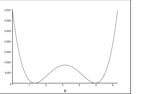
Figure 2: $\lambda^{-1}a^{3}{\cal E}_{\theta}^{(1)}(a)$ as a function of $\theta$ for a massless field in ($3+1$) dimensions.

By taking the limit $m\to 0$ in Eq. (15) we also recover results found in the literature for the periodic ($\theta=0$) and antiperiodic ($\theta=\pi$) boundary conditions [8].

References

[1] P. F. Borges, H. Boschi-Filho, and C. Farina,
Mod. Phys. Lett. A 13, 843 (1998);
Mod. Phys. Lett. A 14, 1217 (1999).
[2] H. Boschi-Filho and C. Farina,
Phys. Lett. A 205, 255 (1995).
[3] A. A. Actor, Int. J. Mod. Phys. A 17, 835 (2002).
[4] F. A. Barone, R. M. Cavalcanti, and C. Farina,
in Proceedings of the XXIII Brazilian National Meeting on
Particles and Fields,
http://www.sbf1.if.usp.br/eventos/enfpc/
xxiii/procs/RES142.pdf
[hep-th/0301238].
[5] F. A. Barone, R. M. Cavalcanti, and C. Farina,
hep-th/0306011.
[6] M. V. Cougo-Pinto, C. Farina, J. F. M. Mendes, and
M. S. Ribeiro, in Proceedings of the XX Brazilian National Meeting
on Particles and Fields, http://www.sbf1.if.usp.br/
eventos/enfpc/xx/procs/res265/.
[7] I. S. Gradshteyn and I. M. Ryzhik,
Table of Integrals, Series, and Products, 6th. ed.
(Academic Press, San Diego, 2000) pp. 1031–1032.
[8] D. J. Toms, Phys. Rev. D 21, 2805 (1980);
M. Krech and S. Dietrich, Phys. Rev. A 46, 1886 (1992).