A Scale Invariance due to Compositeness Condition in the Induced Gauge Theory

Abstract

The scale invariance of the coupling constant in the induced gauge theory due to its compositeness condition is demonstrated in the renormalization group flow of the finite-cutoff gauge theory at the leading order in $1/N$, where $N$ is the number of the matter fermion species.

From theoretical points of view, the gauge fields can be dynamically induced as composite even without preparing them as fundamental objects. The idea of the composite gauge bosons are applied to QED [1], hadron physics [2], the electroweak theory [3, 4, 5], QCD [4, 6], induced gravity [7], braneworld [8] the theory of hidden local symmetry [9] etc. Some people observe that gauge structures emerge in connection with quantization on non-trivial sub-manifolds [10]. Gauge fields are also induced associated with geometric (Berry) phases [11] which appear in the optical, molecular, solid state, nuclear, cosmological and various physical systems [12, 13, 14].

In these models, we expect that the gauge fields become dynamical propagating fields through the quantum fluctuations of the matters. Unfortunately these models are not renormalizable. A powerful way to analyze such models is to rely on their equivalence to the ordinary gauge theory under the compositeness condition (CC), $Z_{3}=0$ [15], where $Z_{3}$ is the wave-function renormalization constant of the gauge field. In recent years, Hattori and one of the present authors (K. A.) investigated theoretical aspects of the CC, and observed a complementarity between gauge boson compositeness and asymptotic freedom of the theory [16]. The renormalization group (RG) approaches provide important clues to investigate these model. In fact many people attempted to study and apply the method [17]. Most of them, however, considered the limit of the infinite momentum cutoff, which necessitates some additional assumptions, such as existence of fixed point and ladder approximation. Here, we take the momentum cutoff as a large but finite physical parameter, and make no further assumptions. In the previous paper, we analyzed the RG flow of the Yukawa model and the scale invariance of the coupling constants in the Nambu-Jona-Lasinio model [18]. In this letter, we show scale invariance of the coupling constant in the induced gauge theory due to its compositeness condition at the leading order in $1/N$, where $N$ is the number of the fermion species. We demonstrate it in the renormalization group flow of the finite-cutoff gauge theory which includes the induced gauge theory as a special case.

We consider the induced (composite) gauge fields $V_{\mu}$ described by the Lagrangian

$${\cal L}_{\rm comp}=\overline{\Psi}(i\!\not\!\partial-\not\!V-M)\Psi$$ (1)

where $\Psi=(\Psi_{1},\Psi_{2},\cdots,\Psi_{N})$ are $N$ fermions, $M$ is the mass of $\Psi$. Classically $V_{\mu}$ is not an independent dynamical variable since it has no kinetic term. Its Euler equation, however, imposes a constraint, giving rise to interactions among $\Psi$, which supply the kinetic term of $V_{\mu}$ through their quantum fluctuations. Thus $V_{\mu}$ is interpreted as a quantum composite field. The form of the Lagrangian (1) is the common essential step in the various theories of the induced (composite) gauge field [1, 2, 3, 4, 5, 6, 7, 8, 9, 10, 11, 12, 13, 14]. We want to show that the coupling constant $g$ is independent of the scale.

In order to see it, we consider the Abelian gauge theory for the gauge boson $A^{0}_{\mu}$ and $N$ matter fermions $\psi^{0}=(\psi^{0}_{1},\psi^{0}_{2},\cdots,\psi^{0}_{N})$ with the following Lagrangian

$${\cal L}_{\rm G}=-{1\over 4}(\partial_{\mu}A^{0}_{\nu}-\partial_{\nu}A^{0}_{\mu})^{2}+\overline{\psi^{0}}(i\!\not\!\partial-g_{0}\not\!\!A^{0}-m_{0})\psi^{0}$$ (2)

where $m_{0}$ is the bare mass of $\psi^{0}$, and $g_{0}$ is the bare coupling constant. We adopt the dimensional regularization where we consider everything in $d(=4-2\varepsilon)$ dimensional spacetime with small but non-vanishing $\varepsilon$. By them we are not considering ”the theory at the $d(=4-2\varepsilon)$”, but that at $d=4$ with the momentum cutoff described by the scheme. The parameter $\varepsilon$ roughly corresponds to $1/\log\Lambda$ with the momentum cutoff $\Lambda$. To absorb the divergences of the quantum loop diagrams due to (2), we renormalize the fields, the mass, and the coupling constants as

$$\psi^{0}=\sqrt{Z_{2}}\psi,\ \ \ A_{\mu}^{0}=\sqrt{Z_{3}}A_{\mu},\ \ \ Z_{2}m_{0}^{2}=Z_{m}m^{2},\ \ \ Z_{2}\sqrt{Z_{3}}g_{0}={Z_{1}}g\mu^{\varepsilon},\ \ \ \ \$$ (3)

where $\psi$, $A_{\mu}$, $m$, and $g$ are the renormalized fields, mass, and coupling constants, respectively, $Z_{1}$, $Z_{2}$, $Z_{3}$, and $Z_{m}$ are the renormalization constants, and $\mu$ is a mass scale parameter to make $g$ dimensionless. Then the Lagrangian ${\cal L}_{\rm G}$ becomes

$${\cal L}_{\rm G}=-{1\over 4}Z_{3}(\partial_{\mu}A_{\nu}-\partial_{\nu}A_{\mu})^{2}+Z_{2}\overline{\psi}i\!\not\!\partial\psi+Z_{1}g\mu^{\varepsilon}\overline{\psi}\not\!\!A_{\mu}\psi+Z_{m}m\overline{\psi}\psi.$$ (4)

As the renormalization condition, we adopt the minimal subtraction scheme, where, as the divergent part to be absorbed into in the renormalization constants, we retain all the negative power terms in the Laurent series in $\varepsilon$ of the divergent (sub)diagrams. Then the parameter $\mu$ is interpreted as the renormalization scale. Since the coupling constants are dimensionless, the renormalization constants depend on $\mu$ only through $g$, but do not explicitly depend on $\mu$.

We can see that the Lagrangian (4) coincides with the Lagrangian (1) if

$$Z_{3}=0,\ \ \ Z_{1}\not=0,\ \ \ Z_{2}\not=0.$$ (5)

The condition (5) is the “compositeness condition” (CC) [15] which imposes relations among the coupling constant $g$, the mass $m$, and the cutoff parameter $\varepsilon$ in the gauge theory so that it reduces to the induced (composite) gauge theory. The perturbative calculation shows that $g\rightarrow 0$ as $\varepsilon\rightarrow 0$ at each order, and the theory becomes trivial free theory. Therefore we fix the cutoff $\Lambda=\mu e^{1/\varepsilon}$ at some finite value. We can read off from (1) and (4) that the fields and masses should be connected by the relations

$$\Psi=\sqrt{Z_{2}}\psi,\ \ V_{\mu}={Z_{1}g\mu^{\varepsilon}\over Z_{2}}A_{\mu},\ \ Z_{2}M=Z_{m}m.$$ (6)

In terms of the bare parameters the CC (5) corresponds to the limit

$$g_{0}\rightarrow\infty.\ \ \ \$$ (7)

This behaviors may look singular at first sight, but they are of no harm because they are unobservable bare quantities.

Let us consider RG equation in the gauge theory with special cares on the finite cutoff. In our case, it amounts to fix $\varepsilon=(4-d)/2$ at some non-vanishing value. The beta functions and the anomalous dimensions are defined as

$$\beta_{g}^{(\varepsilon)}(g)=\mu{\partial g\over\partial\mu},$$ (8)

$$\gamma_{A_{\mu}}^{(\varepsilon)}(g)={1\over 2}\mu{\partial\ln Z_{\phi}\over\partial\mu}\ ,\ \ \ \ \gamma_{\psi}^{(\varepsilon)}(g)={1\over 2}\mu{\partial\ln Z_{\psi}\over\partial\mu}\ ,$$ (9)

where the differentiation $\partial/\partial\mu$ performed with $g_{0}$ and $\varepsilon$ fixed. Operating $\mu(\partial/\partial\mu)$ to the equations in (3) we obtain

$$\left[\beta_{g}^{(\varepsilon)}{\partial\over\partial g}+\varepsilon\right]gJ=0,\ \ \ \$$ (10)

where $J=Z_{1}/(Z_{2}\sqrt{Z_{3}})$. Comparing the residues of the poles at $\varepsilon=0$, we obtain

$$\beta_{g}^{(\varepsilon)}=-\varepsilon g+g{\cal D}J_{1}$$ (11)

where ${\cal D}=g(\partial/\partial g)$, and $J_{1}$ is the residue of the simple pole of $J$. On the other hand the anomalous dimensions are given by

$$\gamma_{A_{\mu}}^{(\varepsilon)}=-{1\over 2}{\cal D}Z_{3,1},\ \ \ \ \gamma_{\psi}^{(\varepsilon)}=-{1\over 2}{\cal D}Z_{2,1},$$ (12)

where $Z_{3,1}$ and $Z_{2,1}$ are the residues of the simple poles of $Z_{3}$ and $Z_{2}$, respectively. We can read off from (11) and (12) that $\beta_{g}^{(\varepsilon)}$ depends on the cutoff only through the first terms $-\varepsilon g$ of the expression, while $\gamma^{(\varepsilon)}$’s are independent of $\varepsilon$. We should be careful not to neglect the cutoff dependence of $\beta_{g}^{(\varepsilon)}$.

The CC $Z_{3}=0$ (eq.(5)) with (14) connects the terms with different order in the coupling constants. Accordingly, the expansion in the coupling constants fails in the case of the induced gauge theory. Therefore we instead adopt the $1/N$ expansion by assigning

$$g^{2}\sim 1/N,\ \ \ \$$ (13)

which does not mix the different orders in CC (5). Explicit calculations at the leading order in $1/N$ show

$$Z_{3}=1-{Ng^{2}\over 12\pi^{2}\varepsilon}\ ,\ \ \ Z_{1}=Z_{2}=1.\ \ \$$ (14)

Applying (13) and (14) to (11) and (12), we get, at the leading order in $1/N$,

$$\beta_{g}^{(\varepsilon)}=-\varepsilon g+{Ng^{3}\over 12\pi^{2}},\ \ \ \gamma_{A_{\mu}}^{(\varepsilon)}={Ng^{2}\over 12\pi^{2}}\ ,\ \ \ \gamma_{\psi}^{(\varepsilon)}=0.\ \ \$$ (15)

The RG equation with the functions in (15) determine the flow of the various quantities with the increasing scale $\mu$.

The RG equations for the coupling constant $g$ are given by (8) with (15), and are solved as

$$g^{2}={1\over\displaystyle{N\over 12\pi^{2}\varepsilon}+{\mu^{2\varepsilon}\over g_{0}^{2}}}\ ,$$ (16)

where the integration constant has been determined in accordance with (3). We can confirm the results by deriving (16) directly from (3) with (14). In fact the RG flow of coupling constant is entirely determined by (3). In the infinite cutoff limit $\varepsilon\rightarrow 0$, (16) becomes

$$g^{2}={1\over\displaystyle a-{N\ln\mu^{2}\over 12\pi^{2}}}\ ,$$ (17)

with $a=N/16\pi^{2}\varepsilon+1/g_{0}^{2}$ kept fixed.

Let us consider the properties of the induced gauge theory in the RG flow of the cutoff gauge theory. In the limit of induced gauge theory (7), the solution (16) reduces to

$$g^{2}={12\pi^{2}\varepsilon\over N}\equiv g^{2}_{\rm comp},\ \ \ \$$ (18)

This can also be derived by directly solving the compositeness condition $Z_{3}=0$ in (5) with (14). The coupling constant (18) for the induced gauge theory is independent of the scale parameter $\mu$. Namely, the induced gauge theory is at the fixed point (18) in the RG flow of the cutoff gauge theory.

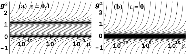
Figure 1: The RG flow of $g^{2}$ vs $\mu$ at (a) finite cutoff and (b) infinite cutoff.

Fig. 1 shows the $\mu$-dependence of $g^{2}$ for various values of $g_{0}^{2}$, (a) at finite cutoff $\varepsilon=0.1$, and (b) at the infinite cutoff limit $\varepsilon=0$. The number of the fermion species $N$ is typically taken as 10. If $g_{0}^{2}>0$, then $0<g^{2}<g^{2}_{\rm comp}$, and $g^{2}\rightarrow g^{2}_{\rm comp}-0$, as $\mu\rightarrow+0$, while $g^{2}\rightarrow+0$ as $\mu\rightarrow\infty$. If $g_{0}^{2}<0$ and $0<\mu<(-Ng_{0}^{2}/16\pi^{2}\varepsilon)^{1/2\varepsilon}\equiv\mu_{\rm c}$, then $g^{2}>g^{2}_{\rm comp}$ and $g^{2}\rightarrow g^{2}_{\rm comp}+0$, as $\mu\rightarrow+0$, while $g^{2}\rightarrow\infty$ as $\mu\rightarrow\mu_{\rm c}-0$. If $g_{0}^{2}<0$ and $\mu>\mu_{\rm c}$, then $g^{2}<0$, and $g^{2}\rightarrow-\infty$ as $\mu\rightarrow\mu_{\rm c}+0$, while $g^{2}\rightarrow-0$ as $\mu\rightarrow\infty$. Thus the $g^{2}=g^{2}_{\rm comp}$ is an infrared fixed point, and $g^{2}=0$ is an ultraviolet fixed point. The region $g^{2}<g^{2}_{\rm comp}$ is asymptotically free, though the region $g^{2}<0$ is unphysical because the Lagrangian is not hermitian. On the other hand, in the region $g^{2}>g^{2}_{\rm comp}$, $g^{2}$ blows up at $\mu=\mu_{\rm c}$, though it should not be taken serious, because the expansion itself is no longer justified in the region where $g^{2}$ is large. In the infinite cutoff limit $\varepsilon\rightarrow 0$, the fixed point $g^{2}=g^{2}_{\rm comp}$ moves to and fuses with the other fixed point $g^{2}=0$. Accordingly the physical asymptotic-freedom region $0<g^{2}<g^{2}_{\rm comp}$ disappears, leaving only the region where the coupling constant blows up.

Thus the induced gauge theory is at a fixed point in the RG flow of the cutoff gauge theory. The coupling constant in the induced gauge theory is scale-invariant, and does not run with the scale parameter. We can trace back the reason of scale invariance to the fact that beta functions vanish due to the compositeness condition. In fact if we substitute the solution (18) of the compositeness condition, the beta function in (15) vanishes. It is further traced back to the fact that the scale invariance of the relation (3) in the limit (7). Thus the scale invariance is expected to hold not only at the leading order in $1/N$, but also at higher order. We are planning to investigate it at the next-to-leading order.

This work is supported by Grant-in-Aid for Scientific Research, Japanese Ministry of Culture and Science.

References

- [1] W. Heisenberg, Rev. Mod. Phys. 29 (1957) 269; J. D. Bjorken, Ann. Phys. 24 (1963) 174; I. Bialynicki-Birula, Phys. Rev. 130 (1963) 465; D. Lurié and A. J. Macfarlane, Phys. Rev. 136 (1964) B816.
- [2] T. Eguchi and H. Sugawara, Phys. Rev. D10 (1974) 4257; H. Kleinert, Phys. Lett. 59B (1975) 163; T. Kugo, Prog. Theor. Phys. 55 (1976) 2032; T. Kikkawa, Prog. Theor. Phys. 56 (1976) 947; A. Chakrabarti and B. Hu, Phys. Rev. D13 (1976) 2347.
- [3] P. Budini, Lett. Nuovo Cim. 9 (1974) 493; P. Budini and P. Furlan, Nuovo Cim. 30A (1975) 63; T. Saito and K. Shigemoto, Prog. Theor. Phys. 57 (1977) 242.
- [4] H. Terazawa, Y. Chikashige and K. Akama, Phys. Rev. D15 (1977) 480; K. Akama and T. Hattori, Phys. Rev. D39 (1989) 1992; D40 (1989) 3688; K. Akama, T. Hattori and M. Yasuè, Phys. Rev. D 42 (1990), 789; 43 (1991) 1702.
- [5] M. Suzuki, Phys. Rev. D37 (1988) 210; S. Ishida and M. Sekiguchi, Prog. Theor. Phys. 86 (1991) 491; K. Akama and T. Hattori, Int. J. Mod. Phys. A9 (1994) 3503; B. S. Balakrishna and K. T. Mahanthappa, Phys. Rev. D49 (1994) 2653; D52 (1995) 2379; A. Galli, Phys. Rev. D51 (1995) 3876; Nucl. Phys. B435 (1995) 339.
- [6] V. A. Kazakov and A. A. Migdal, Nucl. Phys. B397 (1993) 214.
- [7] A. D. Sakharov, Dokl. Akad. Nauk SSSR 177 (1967) 70 [Sov. Phys. Dokl. 12 (1968) 1040]; K. Akama, Y. Chikashige and T. Matsuki, Prog. Theor. Phys. 59 (1978) 653; K. Akama, Y. Chikashige, T. Matsuki and H. Terazawa, Prog. Theor. Phys. 60 (1978) 868; K. Akama, Prog. Theor. Phys. 60 (1978) 1900; Prog. Theor. Phys. 61 (1979), 687; Phys. Rev. D24 (1981), 3073; S. L. Adler, Phys. Rev. Lett. 44 (1980) 1567; A. Zee, Phys. Rev. D23 (1981) 858; D. Amati and G. Veneziano, Phys. Lett. 105B (1981) 358; Nucl. Phys. B240 (1982), 451; K. Akama and I. Oda, Phys. Lett. B 259 (1991), 431; Nucl. Phys. B 397 (1993) 727.
- [8] K. Akama, Lect. Notes in Phys. 176 (1983) 267; Prog. Theor. Phys. 78, 184 (1987); 79, 1299 (1988); 80 (1988) 935; hep-th/0307240 (2003); G. Dvali, G. Gabadadze, and M. Porrati, Phys. Lett. B485 (2000) 208; K. Akama and T. Hattori,Mod. Phys. Lett. A 15 (2000) 2017.
- [9] E. Cremmer and B. Julia, Phys. Lett. 80B (1978) 48; Nucl. Phys. B159 (1979) 141; M. Bando, T. Kugo, S. Uehara, K. Yamawaki and T. Yanagida, Phys. Rev. Lett. 54 (1985) 1215;
- [10] N. P. Landsman and N. Linden, Nucl. Phys. B365 (1991) 121; D. McMullan and I. Tsutsui, Phys. Lett. B320 (1994) 287; Ann. Phys. 237 (1995) 269; S. Tanimura and I. Tsutsui, Mod. Phys. Lett. A10 (1995) 2607.
- [11] S. Pancharatnam, Proc. Indian Acad. Sci. 44A 247; G. Herzberg and H. C. Longuet-Higgins, Disc. Farad. Soc. 35 (1963) 77; C. A. Mead and D. G. Truhlar, J. Chem. Phys. 70(05) (1979) 2284; M. V. Berry, Proc. R. Soc. London Ser. A392 (1984) 45.
- [12] G. Delacrétaz et al, Phys. Rev. Lett. 56 (1986) 2598; A. Tomita and R. Chiao, Phys. Rev. Lett. 57 (1986) 937; D. Suter et al, Mol. Phys. 61 (1987) 1327.
- [13] A. Yu. Smirnov, Phys. Lett. B260 (1991) 161; S. Forte, Mod. Phys. Lett. A6 (1991) 3153; H. K. Lee, M. A. Nowak, M. Rho and I. Zahed, Ann. Phys. B227 (1993) 175; Y. Aharanov et al, Phys. Rev. Lett 73 (1994) 918; A. Corichi and M. Pierri, Phys. Rev. D51 (1995) 5870.
- [14] K. Kikkawa, Phys. Lett. B297 (1992) 89; T. Hatsuda and H. Kuratsuji, UTHEP-286 (1994); K. Kikkawa and H. Tamura, Int. J. Mod. Phys. A10 (1995) 1597.
- [15] B. Jouvet, Nuovo Cim. 5 (1956) 1133; M. T. Vaughn, R. Aaron and R. D. Amado, Phys. Rev. 124 (1961) 1258; A. Salam, Nuovo Cim. 25 (1962) 224; S. Weinberg, Phys. Rev. 130 (1963) 776; B. W. Lee, K. T. Mahanthappa, I. S. Gerstein and M. L. Whippman, Ann. Phys. B28 (1964) 466; J. Lemmon and K. T. Mahanthappa, Phys. Rev. D13 (1976) 2907; T. Eguchi, Phys. Rev. D14 (1976) 2755; D17 (1978) 611; H. Kleinert, in Understanding the fundamental constituents of matter, proceedings, 1976 Erice Summer School, ed. A. Zichichci (Plenum Publishing Corporation, 1978), 289; K. Shizuya, Phys. Rev. D21 (1980) 2327;
- [16] K. Akama, Phys. Rev. Lett. 76, 184 (1996); Nucl. Phys. A 629 (1998), 37C; K. Akama and T. Hattori, Phys. Lett. B392, 383 (1997); B445, 106 (1998); hep-th/0310236 (2003).
- [17] T. Eguchi, Ref. [15]; K. Akama and T. Hattori, Ref. [4]; J. Zinn-Justin, Nucl. Phys. B367 (1991) 105; D. Lureié and G.B. Tupper, Phys. Rev. D47 (1993) 3580; J. A. Gracey, Phys. Lett. B308 (1993) 65; B342 (1995) 297.
- [18] K. Akama, hep-th/0310183 (2003).