Quarkonium from the Fifth Dimension

Abstract:

Adding fundamental matter of mass $m_{Q}$ to ${\cal N}=4$ Yang Mills theory, we study quarkonium, and “generalized quarkonium” containing light adjoint particles. At large ’t Hooft coupling the states of spin $\leq 1$ are anomalously light (Kruczenski et al., hep-th/0304032). We examine their form factors, and show these hadrons are unlike any known in QCD. By a traditional yardstick they appear infinite in size (as with strings in flat space) but we show that this is a failure of the yardstick. All of the hadrons are actually of finite size $\sim\sqrt{g^{2}N}/m_{Q}$, regardless of their radial excitation level and of how many valence adjoint particles they contain. Certain form factors for spin-1 quarkonia vanish in the large-$g^{2}N$ limit; thus these hadrons resemble neither the observed $J/\Psi$ quarkonium states nor $\rho$ mesons.

1 Introduction

The discovery that gauge theory at large ’t Hooft coupling can be described using string theory [1] has given rise to many interesting developments in both fields. The original idea has been extended to purely four-dimensional confining gauge theories [2, 3, 4]. These examples provide the first toy models of QCD whose kinematics is that of the real world. In particular, these theories share with QCD the property of four-dimensional approximate scale invariance in the ultraviolet, as well as confinement in the infrared. Consequently, the differences between these models and QCD are largely due to dynamical, rather than kinematical, issues. Indeed, these theories smoothly become QCD-like when the ’t Hooft coupling is small.

However, most of the theories studied up to now differ from QCD in a significant way: their matter comes in representations with of order $N^{2}$ fields, and they are all neutral under some portion of the center of the gauge group. These differences from QCD are much more important, both kinematically and dynamically, than the fact that many of these theories are supersymmetric. The reasons for this are clear. Quarks in the ${\bf N}$ representation of $SU(N)$ color introduce new features into the $1/N$ expansion; quark pair-production makes confining flux tubes unstable; baryons now appear in the spectrum; and there are new flavor symmetries which may or may not be explicitly or spontaneously broken. Thus the theory without quarks in the ${\bf N}$ representation, supersymmetric or not, differs signficantly from the theory which contains them. It is thus important to the development of these toy models of QCD to introduce matter in the fundamental representation. In the limit where the number of flavors $N_{f}$ is much less than $N$, this was considered in [5, 6, 7]; a simpler method was invented in [8] and studied further in [9, 10]. Still more recently, there has been additional work in other related contexts [11].

One of the obvious objects to study in a theory with quarks is quarkonium. At small ’t Hooft coupling this is just a hydrogenic atom, but at large ’t Hooft coupling the system is highly relativistic. The quarkonium spectrum at large ’t Hooft coupling, in the model studied in [10], is remarkable from the field-theoretic point of view. Its details could not have been guessed from any known theoretical argument or from any aspect of the observed QCD spectrum, and it is profoundly tied up with the representation of the four-dimensional gauge theory as a higher-dimensional string theory. Still more puzzles emerge in states built from a quark, an antiquark, and one or more particles of the much lighter adjoint matter. These states would naively be expected to be qualitatively different in size and structure from pure quarkonium. Instead, it has been found [10] that these states are quite similar to pure quarkonium at large ’t Hooft coupling.

In order to gain better insight into the structure and couplings of these bound states, we have computed some of their form factors and transition matrix elements with respect to various conserved currents. Fourier transforming the form factors, we find that all the hadrons are more or less the same size — larger than one would expect for quarkonium, and smaller than one would expect when adjoint matter is bound to the quark-antiquark system. Our results do not solve any mysteries, but they do raise interesting questions and suggest other calculations to do in future. We are also led to a conjecture about the substructure of the hadrons.

We review the results of [8] and [10] in the following section. Sections 3, 4 and 5 contain our methodology, a summary of our results, and the detailed computations. The physical implications of our results are discussed in Section 6.

2 Preliminaries

The introduction of matter in the fundamental representation into theories with gravitational dual descriptions has been considered by a number of authors [5, 6, 7]. However, theoretical prejudices about the appropriate systems, and technical difficulties with those that were investigated, delayed progress for some time. Recently, Karch and Katz [8] cut the Gordion knot, pointing out that many interesting questions could be addressed in the simplest possible brane construction with fundamental matter: a small number $N_{f}$ of D7 branes in the vicinity of a large number $N$ of D3 branes.

2.1 The theory in question

The field theory corresponding to this arrangement of branes consists of ${\cal N}=4$ $SU(N)$ Yang-Mills coupled in an ${\cal N}=2$ supersymmetric fashion to $N_{f}$ hypermultiplets in the fundamental representation. We will write the ${\cal N}=4$ vector multiplet as an ${\cal N}=1$ vector multiplet $W_{\alpha}$ and three chiral multiplets $\Phi_{1},\Phi_{2},\Phi_{3}$ in the adjoint represntation. The hypermultiplets are given as ${\cal N}=1$ chiral multiplets $Q^{r},\tilde{Q}_{r}$ ($r=1,\dots,N_{f}$) in the fundamental and antifundamental representation respectively, and we will call their scalars “squarks” and “antisquarks” and their fermions “quarks” and “antiquarks.” Written in ${\cal N}=1$ language, the theory consists of kinetic terms for all the fields (along with ${\cal N}=1$ superpartners of the kinetic terms) and a superpotential of the form

$$W=\sqrt{2}\ {\rm tr}\Big{(}[\Phi_{1},\Phi_{2}]\Phi_{3}\Big{)}+\sum_{r=1}^{N_{f}}Q^{r}\Phi_{3}\tilde{Q}_{r}+m_{r}Q^{r}\tilde{Q}_{r}$$

where $m_{r}$ is the mass of hypermultiplet $r$ and the trace is over color indices.

The theory has an $SO(4)\approx SU(2)\times SU(2)$ symmetry, consisting of an $SU(2)_{\Phi}$ symmetry rotating $\Phi_{1}$ and $\Phi_{2}$ and an $SU(2)_{R}$ ${\cal N}=2$ R-symmetry. The charges of the fields under these symmetries are shown in the table, where we write $\Phi_{1}=X^{4}+iX^{5}$, $\Phi_{2}=X^{6}+iX^{7}$, and $\Phi_{3}=X^{8}+iX^{9}$, the adjoint fermions as $\lambda_{1}$, $\lambda_{2}$, $\lambda_{3}$, $\lambda_{4}$, and the quarks as $\psi$, $\tilde{\psi}$.

	$SU(2)_{\Phi}\times SU(2)_{\cal R}$	$U(1)_{R}$	$U(N_{f})$
$X^{4,\cdots,7}$	$(\frac{1}{2},\frac{1}{2})$	0	1
$X^{8,9}$	$(0,0)$	$\pm 2$	1
$\lambda_{1},\lambda_{2}$	$(\frac{1}{2},0)$	$-1$	1
$\lambda_{3},\lambda_{4}$	$(0,\frac{1}{2})$	$+1$	1
$Q,\tilde{Q}^{\dagger}$	$(0,{\frac{1}{2}})$	0	$N_{f}$
$\psi,\tilde{\psi}^{\dagger}$	$(0,0)$	$\mp 1$	$N_{f}$

The masses $m_{r}$ are the eigenvalues of a matrix which transforms in the adjoint of $U(N_{f})$. If all masses $m_{r}$ are zero, the $U(1)_{R}$ ${\cal N}=1$ R-symmetry is preserved by the superpotential. Nonzero masses break this $U(1)$ R-symmetry, but leave invariant the $SO(4)$. The $U(N_{f})$ is also generally broken by the masses, but if all the masses are equal, as we will assume throughout, $U(N_{f})$ is preserved.

The string dual description of this field theory [8], for large ’t Hooft coupling, is simply given as $N_{f}$ D7 branes placed as probes inside $AdS_{5}\times S^{5}$. Each D7 brane introduces a hypermultiplet of mass $m$, where $m$ is proportional to the minimum value of the $AdS_{5}$ radial coordinate $r$ to which the D7 brane descends. At any larger and fixed value of $r$, the D7 brane fills out an $S^{3}$ subspace of the $S^{5}$. We will give more details on this brane construction below.

The theory’s reduced supersymmetry is of little concern, but it does seem at first to have a serious dynamical problem. The gauge coupling now has a positive beta function, making the ultraviolet definition of the theory problematic, and potentially destroying any hope of making sense of the theory using gauge-string duality. In particular, the dilaton is no longer constant. Where the dilaton (equivalently, the gauge coupling of the gauge theory) becomes of order 1, one ought to do an S-duality transformation; but this would turn the D7-branes into magnetic 7-branes, which are very difficult to handle.

However, the gauge beta function is very small. In particular, the beta function for $g_{YM}$ is of order $g_{YM}^{3}N_{f}$, so the beta function for the ’t Hooft coupling $\lambda$ is of order $\lambda^{2}N_{f}/N$. Another way to say this is that at large $N$ and small $N_{f}$ this is a naturally “quenched” theory: all quantum effects due to the fundamental matter are parametrically suppressed by $N_{f}/N$. The squarks and quarks are simply probes of the dynamics of the ${\cal N}=4$ sector. From the supergravity point of view, this suppression is essentially the statement that the backreaction, through the variation of the dilaton, metric and other fields, caused by the D7-branes is negligible out to exponentially large $AdS$ radius. Consequently, as Karch and Katz argued, we can study to leading order in $N_{f}/N$ all of the issues that can normally be investigated in quenched QCD, including the spectrum of hadrons.

2.2 The (s)quark-anti(s)quark hadrons

Karch, Katz and Weiner [9] considered the formation of heavy-light mesons in this theory, working at large ’t Hooft coupling $\lambda\gg 1$. They found a number of surprising results, including confinement of quarks without formation of flux tubes (what one might call “Gribov confinement.” [12])

Another natural issue for study is quarkonium, namely bound states of a quark and antiquark of equal mass. At weak coupling (i.e., small $\lambda$) this is simply the problem of the hydrogen atom, but at strong coupling we do not a priori know what to expect.

A seemingly different problem is that of a quark and antiquark bound to one or more of the $\Phi_{i}$ particles. In the simplest D3-D7 system, these particles are massless. An easier system to think about is obtained by giving the $\Phi_{i}$ small bare masses, so that (as in ${\cal N}=1^{*}$[3]) confinement of flux occurs at a distance very long compared to the quarkonium mass and length scales. Then we can imagine stable bound states of a quark, antiquark and some number of the much lighter $\Phi_{i}$ particles. This problem has not been much studied at small ’t Hooft coupling, but one would expect these bound states, in which the quark and antiquark combined must be in the adjoint representation, would be very different in size and shape from the simple quarkonium bound states.

Surprisingly, at large ’t Hooft coupling both problems can be addressed simultaneously, and on the same footing. This was done by Kruczenski, Mateos, Myers and Winters [10]. They derived the spectrum and higher-dimensional wave functions of mesons consisting of one (s)quark and one anti(s)quark of equal mass, along with some number of massless adjoint particles. The spectrum for states of large spin ($s\gg\sqrt{\lambda}$) was found to be the same as that of hydrogen; this is to be expected, since in this limit the (s)quarks move nonrelativistically even though the coupling is strong. For states of lower spin it was shown that the spectrum has a Regge-like relation betweeen mass and spin: $m^{2}\propto s$. And states of spin $1$, $\frac{1}{2}$ and 0 were found to be extraordinarily deeply bound — so deep that the mass of the hadron is a tiny fraction of the mass of its (s)quark constituents. It is these anomalously light states of low spin — states that are described in the string theory variables by modes of massless higher-dimensional fields — that are the focus of this article. We now review their properties in detail.

We generally follow the setup in [8]. The near-horizon geometry of $N$ D3-branes filling the 0123 directions of the ten-dimensional space, and placed at the origin of the 456789 coordinates, is given by $AdS_{5}\times S^{5}$. We write the metric on the Poincare’ patch variously as

$$ds^{2}={r^{2}\over R^{2}}(dx^{\mu})^{2}+{R^{2}\over r^{2}}dr^{2}+R^{2}d\Omega_{5}^{2}={r^{2}\over R^{2}}\eta_{{\mu\nu}}dx^{\mu}dx^{\nu}+\sum_{c=4}^{9}{R^{2}\over r^{2}}(dx^{c})^{2}$$

where $c=4,5,6,7,8,9$, $\mu=0,1,2,3$, $r^{2}\equiv{\sum_{c}(x^{c})^{2}}$, and $R^{2}=\alpha^{\prime}\sqrt{4\pi g_{s}N}$. Note $r=0$ is the horizon of $AdS$ and $r=\infty$ is its boundary. The D7-branes fill the 01234567 directions; each is placed at some position $x^{8}+ix^{9}=m_{Q}\alpha^{\prime}$. We will make all the masses equal in this paper, so without loss of generality we can take the masses to be real ($x^{8}=m_{Q}\alpha^{\prime}\equiv L$, $x^{9}=0$.) The induced metric on the D7-branes is then

$$ds^{2} = {r^{2}\over R^{2}}\eta_{{\mu\nu}}dx^{\mu}dx^{\nu}+\sum_{c=4}^{7}{R^{2}\over r^{2}}(dx^{c})^{2}$$ (1)

$$= \frac{L^{2}}{R^{2}}(\varrho^{2}+1)\eta_{\mu\nu}dx^{\mu}dx^{\nu}+\frac{R^{2}}{\varrho^{2}+1}d\varrho^{2}+R^{2}\frac{\varrho^{2}}{\varrho^{2}+1}d\Omega_{3}^{2}\ ,$$ (2)

where $\varrho^{2}=\frac{r^{2}}{L^{2}}-1$, and the $S^{3}$ involves the angular coordinates in the four-dimensional space spanned by $x^{4},x^{5},x^{6},x^{7}$.

We will use various coordinates for our calculations which we summarize here:

$$v=(L/r)^{2}\ ,\ w=1-v\ ;\ \varrho^{2}=v^{-1}-1=\frac{w}{1-w}\ .$$ (3)

Note the boundary of the space is located at $r=\infty$, $\rho=\infty$, $v=0$ and $w=1$, whereas the point on the D7-brane which is closest to the $AdS$ horizon at $r=0$ is at $r=L$, $\rho=0$, $v=1$ and $w=0$.

It is useful to define an overall mass scale

$$m_{h}\equiv L/R^{2}=m_{Q}/\sqrt{4\pi g_{s}N}=m_{Q}/\sqrt{\lambda}\ .$$

Barred quantities will be defined relative to $m_{h}$ — for instance, we will often use dimensionless momenta $\bar{q}\equiv\sqrt{|q^{2}|}/m_{h}$ and dimensionless masses $\bar{m}=m/m_{h}$.

There are two real scalar fields and one gauge field on the D7 brane worldvolume; theses are the massless modes of the open strings whose ends are on the D7-branes. If there are $N_{f}$ D7-branes, there are $N_{f}^{2}$ such fields, transforming in the adjoint representation of $U(N_{f})$. The modes of the gauge field, when reduced to five dimensions, break up into spin-one and spin-zero modes in five dimensions. The spin-one modes are associated with the $U(N_{f})$ flavor current, and operators built by adding $\Phi$ fields to the current:

$$(Q^{{\dagger}}\Phi^{\ell}Q-\tilde{Q}\Phi^{\ell}\tilde{Q}^{{\dagger}})_{\theta\bar{\theta}}=Q^{{\dagger}}\Phi^{\ell}\partial^{\mu}Q+\psi^{{\dagger}}_{Q}\Phi^{\ell}\sigma^{\mu}\psi_{Q}-\tilde{Q}\Phi^{\ell}\partial^{\mu}\tilde{Q}^{{\dagger}}+\cdots$$ (4)

where $\Phi^{\ell}$ stands for any product of $\Phi_{1}$ and $\Phi_{2}$ which is a symmetric and traceless representation under $SO(4)$. These operators have conformal dimension $\Delta_{1}\equiv\ell+3$ and transform as $\left(\frac{\ell}{2},\frac{\ell}{2})\right.$ under $SO(4)\approx SU(2)_{\Phi}\times SU(2)_{R}$, and as adjoint under $U(N_{f})$.

When these operators act on the vacuum they can create a spin-one bound state of a $Q$, a $\tilde{Q}$, and $\ell$ $\Phi$ particles (plus any number of gluons, gluino pairs, and $\Phi$–anti-$\Phi$ pairs, of course.) In particular, for $\ell=0$ this is a spin-one quarkonium state, much the same as the J/$\psi$ or the $\Upsilon$ in QCD. The bound state spectrum, and the bulk wave functions of the individual bound states, were computed in [10], where they were termed “type $II$”. These hadrons are modes of the 8-dimensional gauge boson $A_{M}$, of the form

$$A_{\rho}=0,\quad A_{\alpha}=0,\quad A_{\mu}=\zeta_{\mu}\phi^{II}(\rho)e^{ik\cdot x}\mathcal{Y}^{\ell}(S^{3}),\qquad k\cdot\zeta=0$$ (5)

$$\phi^{II}_{\ell,n} = (C_{\ell n}^{II}/R^{2})\varrho^{\ell}(1+\varrho^{2})^{-1-n-\ell}F(-n,-1-n-\ell;\ell+2;-\varrho^{2})$$

$$= (C_{\ell n}^{II}/R^{2})w^{\ell/2}(1-w)^{-\ell/2}F(-1-n-\ell,2+n+\ell;\ell+2;w)$$

$$= (\hat{C}_{\ell n}^{II}/R^{2})v^{(\ell+2)/2}(1-v)^{\ell/2}P_{n}^{(\ell+1,\ell+1)}(2v-1)\ ,$$

where $n\geq 0$, $\ell\geq 0$,

$$C_{\ell n}^{II}=\sqrt{2(2n+2\ell+3){{n+2\ell+2}\choose{\ell+1}}{{n+\ell+1}\choose{\ell+1}}}={{n+\ell+1}\choose{\ell+1}}\hat{C}_{\ell n}^{II}\ .$$

Here $P_{n}^{(\alpha,\beta)}(x)$ denotes a Jacobi polynomial. The masses of these states are

$$M_{II}^{2}=4m_{h}^{2}(n+\ell+1)(n+\ell+2)\ ,$$

where again $m_{h}\equiv L/R^{2}=m_{Q}(\lambda)^{-1/2}$. By coincidence the $\ell=0$ states also appear in the model of [13].

Another mode which is easy to identify is the mode $I-$ in [10], whose conformal dimension is $\Delta_{0}\equiv\ell+1\ (\ell\geq 1)$, and which transforms as $\left(\frac{\ell-1}{2},\frac{\ell+1}{2}\right)$ under $SO(4)\approx SU(2)_{\Phi}\times SU(2)_{R}$. For $\ell=1$ it has dimension 2 and is a triplet under $SU(2)_{R}$. This uniquely picks it out as a multiplet containing the ${\cal N}=1$ chiral operator

$$(\tilde{Q}\Phi^{\ell-1}Q)_{\theta,\bar{\theta}=0}=\tilde{Q}\Phi^{\ell-1}Q+\cdots$$ (6)

along with other modes related by $SO(4)$ (mainly given by replacing $Q$ with $\tilde{Q}^{\dagger}$, $\Phi_{1}$ with $\Phi_{2}$ or $\Phi_{1}^{\dagger}$, etc.) The mode $I-$ is a mode of the 8-dimensional gauge field with its component on the $S^{3}$ nonzero:

$$A_{\mu}=0,\quad A_{\rho}=0,\quad A_{\alpha}\ =\phi^{I-}(\rho)e^{\ ik\cdot x}\mathcal{Y}_{\alpha}^{\ell,-}(S^{3})$$ (7)

$$\phi^{I-}_{\ell,n} = (C^{I}_{\ell n}/L)\varrho^{\ell+1}(1+\varrho^{2})^{-1-n-\ell}F(-n,1-n-\ell;\ell+2;-\varrho^{2})$$

$$= (C^{I}_{\ell n}/L)w^{\frac{\ell+1}{2}}(1-w)^{-(\ell-3)/{2}}F(1-n-\ell,2+n+\ell;\ell+2;w)$$

$$= (\hat{C}^{I}_{\ell n}/L)v^{(\ell+1)/2}(1-v)^{(\ell+1)/2}P_{n}^{(\ell+1,\ell-1)}(2v-1)$$

where $n\geq 0$, $\ell\geq 1$, and

$$C_{\ell n}^{I}=\sqrt{2(2n+2\ell+1){{n+2\ell}\choose{\ell+1}}{{n+\ell+1}\choose{\ell+1}}}={{n+\ell+1}\choose{\ell+1}}\hat{C}_{\ell n}^{I}\ .$$

These scalars have masses

$$M_{I-}^{2}=4m_{h}^{2}(n+\ell)(n+\ell+1)\ .$$

Since we will not use the type $I+$ hadrons, we will henceforth discard the minus sign in $I-$ when referring to these states.

These are the two classes of (s)quark-containing operators and states that we will use for calculations in the rest of this paper. We will also consider matrix elements of the flavor current, which is the operator appearing in Eq. (4) with $\ell=0$. This will require us to know the nonnormalizable mode of the corresponding five-dimensional gauge boson at spacelike $q^{2}=\bar{q}^{2}m_{h}^{2}$, which is of the form

$$\phi^{II}_{non}(w;\alpha)=\frac{\pi\alpha(1+\alpha)}{\sin(\pi\alpha)}F(-\alpha,1+\alpha;2;w),$$ (8)

where $\alpha=\frac{1}{2}\left(-1+\sqrt{1-\bar{q}^{2}}\right)$.

For completeness we briefly comment about the other classes of hadrons appearing in [10]. There is a set of complex operators $\psi_{\tilde{Q}}\Phi^{\ell-1}\psi_{Q}+\cdots$ which are obtained from the operators (6) by the action of two supersymmetry generators; these complex modes create the two “scalar modes” in [10]. The type $III$ and type $I+$ hadrons are harder to identify, as there are a number of candidate operators, of which only particular linear combinations are chiral.

2.3 The ${\cal N}=4$ sector

We will also consider certain modes of the ${\cal N}=4$ sector, which appear as states of the ten-dimensional supergravity on $AdS_{5}\times S^{5}$. We will only need the spin-one states created by acting on the vacuum with the $SO(4)$ current $J_{4}^{a\mu}\sim{\rm tr}\ \Phi_{i}^{\dagger}\partial_{\mu}\Phi_{j}(T^{a}_{SO(4)})_{ij}+\cdots$ and the spin-two states given by acting on the vacuum with $T^{\mu\nu}\sim{\rm{\rm tr}}\ F^{\mu}_{\rho}F^{\rho\nu}+\Phi_{i}^{\dagger}\partial^{\mu}\partial^{\nu}\Phi+\cdots$. (The traces are over color indices.) However, it will be convenient to consider also a spin zero operators which has a close relationship with the spin one and two operators. The spin zero operator corresponds to the ten-dimensional metric element which is a singlet under the transformation on the seven brane. Under the breaking $SO(6)\rightarrow SO(4)\times SO(2)$, the traceless symmetric rank two tensor representation $\boldsymbol{2}\boldsymbol{0}$ branches to $(\boldsymbol{1},\boldsymbol{1})\oplus(\boldsymbol{9},\boldsymbol{1})\oplus(\boldsymbol{1},\boldsymbol{2})\oplus(\boldsymbol{4},\boldsymbol{2})$. The singlet corresponds to the dimension-two $SO(4)$–singlet operator ${\cal S}\sim\Phi_{1}^{2}+\Phi_{2}^{2}-2\Phi_{3}^{2}$.

2.3.1 The continuous spectrum of the conformal theory

We will consider the operators whose spins range from zero to two. The non-normalizable mode for the operator with spin $S$ is [14]

$$\left(\frac{L^{2}}{R^{2}v}\right)^{S-1}\frac{(\bar{q}\sqrt{v})^{S}}{S!}K_{S}(\bar{q}\sqrt{v}).$$ (9)

where $\bar{q}=\sqrt{q^{2}}/m_{h}$ and $q^{2}>0$ is spacelike. Note that $L^{2}/R^{2}v$ in the prefactor is the warp factor of the four dimensional part of the metric. It is needed in order to have the correct boundary behavior of the non-normalizable mode.

The $SO(4)$ current is associated under AdS/CFT duality with a five-dimensional gauge boson $\hat{A}$, which descends from the off-diagonal elements of the ten-dimensional metric. In particular, let $v^{a}$ be a Killing vector on the three-sphere which points purely parallel to the D7-brane world-volume (and thus leaves it invariant.) Then the metric elements $h_{\mu a}=\hat{A}_{\mu}v_{a},h_{ra}=\hat{A}_{r}v_{a}$ (where $ds^{2}=ds^{2}_{AdS_{5}\times S^{5}}+h_{\mu a}dx^{\mu}dx^{a}$) define the $SO(4)$ gauge boson on $AdS_{5}$. In radial gauge $\hat{A}_{r}=0$, the non-normalizable modes of $\hat{A}$ at spacelike $q^{2}$ are

$$\hat{A}_{\mu}(q)=\epsilon_{\mu}\bar{q}\sqrt{v}K_{1}(\bar{q}\sqrt{v})\$$ (10)

which are normalized following (9) so that $\hat{A}_{\mu}\to\epsilon_{\mu}$ as $v\to 0$. The corresponding normalizable modes, at specific values of timelike $q^{2}=-|q^{2}|\equiv-m_{h}^{2}\bar{m}^{2}$, are of the form

$$\hat{A}_{\mu}(q)\propto\epsilon_{\mu}\bar{m}\sqrt{v}J_{1}(\bar{m}\sqrt{v})\ .$$ (11)

One can build normalizable wave packets from the normalizable modes, although, just as with plane waves in flat space, there is no normalized version of the modes in (11).

For the spin-two current we need the modes of the traceless $AdS_{5}$ part of the metric. We consider traceless fluctuations $ds^{2}=ds^{2}_{AdS_{5}\times S^{5}}+h_{\mu\nu}dx^{\mu}dx^{\nu}$, $h_{\mu}^{\mu}=0$, in radial gauge $h_{rr}=0,h_{r\mu}=0$. The normalizable modes take the form

$$h_{\mu\nu}(q)\propto\epsilon_{\mu\nu}J_{2}(\bar{m}\sqrt{v})$$ (12)

while the nonnormalizable modes are

$$h_{\mu\nu}(q)=\epsilon_{\mu\nu}\frac{L^{2}}{R^{2}v}\cdot\frac{\bar{q}^{2}v}{2}K_{2}(\bar{q}\sqrt{v})\ .$$ (13)

As $v\rightarrow 0$, the non-normalizable mode approaches $h_{\mu\nu}\rightarrow\epsilon_{\mu\nu}\frac{L^{2}}{R^{2}v}$, which is the four-dimensional warp factor, times a polarization tensor.

Since the ${\cal N}=4$ theory is conformal in the infrared, its spectrum of normalizable modes is continuous: any timelike $q^{2}$ is allowed. We should not think of the normalizable modes as hadrons, but simply as a spectral decomposition of a conformal field.

2.3.2 The discrete spectrum of hadrons of a confining model

However, it will often be useful to consider instead a confining theory, in which the conformal invariance of the ${\cal N}=4$ sector is broken in the deep infrared. For instance, we can imagine the ${\cal N}=4$ sector is deformed into a theory similar to ${\cal N}=1^{*}$ [3], where the ${\cal N}=1$ chiral superfields $\Phi_{1},\Phi_{2},\Phi_{3}$ are given a small mass. This causes confinement to set in at a low scale $\Lambda$. In all known models of this type, the $AdS$ radial coordinate is effectively cut off at $r=r_{min}=\Lambda R^{2}$. Our results will be insensitive to the details of this cutoff, as will become clear, so a crude model will suffice to capture the essence of the physics. In any such model, the flavorless ${\cal N}=4$ sector of the theory will have a discrete spectrum of spin-$s$ ($s\leq 2$) hadrons, with masses of order $n\pi\Lambda$ ($0<n\in{\bf Z}$), and with mode functions given at large $r$ by the normalizable modes of the corresponding bulk fields.

To be definite, we will model confinement through the boundary condition that the ten-dimensional wave function of each hadron satisfies the Neumann condition at $r=r_{min}$, that is, at $v_{max}=m_{h}^{2}/\Lambda^{2}$. In this simple model, the wave functions for the hadrons created by the $SO(4)$ current are precisely those of (11) for $v<v_{max}$, with a quantization condition that only $q^{\mu}$ satisfying $(\sqrt{v_{max}}J_{1}(\bar{m}\sqrt{v_{max}}))^{\prime}=0$, where again $\bar{m}=\sqrt{|q^{2}|}/m_{h}$, are allowed. Thus we have a countably infinite series of modes, with mass $m_{n}=\bar{m}\sqrt{v_{max}}=\zeta_{0;n}$, $n\geq 1$, where $\zeta_{0;n}$ is the $n^{th}$ zero of $J_{0}$. The normalization is obtained from [15]

$$\int_{0}^{v_{max}}dvd^{3}\Omega\,e^{2A}\sqrt{g_{\bot}}g^{MN}A_{M}A_{N}=1,$$ (14)

where

$$ds^{2}=e^{2A}\eta_{\mu\nu}dx^{\mu}dx^{\nu}+ds_{\bot}^{2}.$$

Thus we have a spectrum of states with normalized wave functions

$$\hat{A}_{\mu}(m_{n})=\epsilon_{\mu}\frac{\sqrt{2}\sqrt{v/v_{max}}J_{1}(\zeta_{0;n}\sqrt{v/v_{max}})}{R^{3}J_{1}(\zeta_{0;n})}=\epsilon_{\mu}R^{-3}{\Lambda\over m_{h}}\frac{\sqrt{2v}J_{1}(\bar{m}_{n}\sqrt{v})}{J_{1}(\zeta_{0;n})}\ ,$$ (15)

and masses

$$\bar{m}_{n}\equiv{m_{n}\over m_{h}}={\zeta_{0;n}}{\Lambda\over m_{h}}\underset{\quad n\gg 1}{\longrightarrow}\left(n-\frac{1}{4}\right)\pi{\Lambda\over m_{h}}\ .$$ (16)

We will need the nonnormalizable modes satisfying the same boundary condition, which are (for spacelike $q^{2}=\bar{q}^{2}m_{h}^{2}$)

$$\hat{A}_{\mu}(\bar{q})=\epsilon_{\mu}\bar{q}\sqrt{v}\left\{K_{1}(\bar{q}\sqrt{v})+I_{1}(\bar{q}\sqrt{v})\frac{K_{0}(\bar{q}m_{h}/\Lambda)}{I_{0}(\bar{q}m_{h}/\Lambda)}\right\}.$$ (17)

Similarly, the spin-two hadrons created by $T^{\mu\nu}$ have wave functions given by

$$h_{\mu\nu}(m_{n})=\epsilon_{\mu\nu}\frac{m_{h}\sqrt{2/v_{max}}J_{2}(\zeta_{1;n}\sqrt{v/v_{max}})}{R^{2}J_{2}(\zeta_{1;n})}=\epsilon_{\mu\nu}\frac{\Lambda}{R^{2}}\frac{\sqrt{2}J_{2}(\bar{m}_{n}\sqrt{v})}{J_{2}(\zeta_{1;n})}$$ (18)

with masses

$$\bar{m}_{n}\equiv{m_{n}\over m_{h}}={\zeta_{1;n}}{\Lambda\over m_{h}}\underset{\quad n\gg 1}{\longrightarrow}\left(n+\frac{1}{4}\right)\pi{\Lambda\over m_{h}}\ .$$ (19)

where $\zeta_{1;n}$ are the zeroes of $J_{1}$. The normalization constant is obtained in a similar way as in Eq. (14):

$$\int^{v_{max}}_{0}dvd^{3}\Omega\,e^{2A}\sqrt{g_{\bot}}g^{MN}g^{PQ}h_{MP}h_{NQ}=1\ .$$ (20)

The nonnormalizable modes are now

$$h_{\mu\nu}(\bar{q})=\epsilon_{\mu\nu}\frac{L^{2}}{R^{2}v}\frac{\bar{q}^{2}v}{2}\left\{K_{2}(\bar{q}\sqrt{v})+I_{2}(\bar{q}\sqrt{v})\frac{K_{1}(\bar{q}m_{h}/\Lambda)}{I_{1}(\bar{q}m_{h}/\Lambda)}\right\}\ .$$ (21)

3 Methodology

3.1 Definitions and Notation

We will concern ourselves mainly with the form factors from the hadronic matrix elements of the $U(N_{f})$ flavor current $J^{\mu}_{f}$, the $SO(4)\approx SU(2)_{\Phi}\times SU(2)_{R}$ current $J^{\mu}_{4}$, and the energy-momentum tensor $T^{\mu\nu}$. We will also consider matrix elements of the $SO(4)$-singlet spin-zero dimension-two operator ${\cal S}\propto\Phi_{1}^{2}+\Phi_{2}^{2}-2\Phi_{3}^{2}$, which is part of the conformal ${\cal N}=4$ sector.

We will compute a large number of form factors, so it is important that our notation be clear. When the maximal information needs to be displayed, we will use the following notation for a form factor. Suppose we have a spin-zero (type $I$) or a spin-one (type $II$) initial state with $\ell,n_{1}$ quantum numbers. In our calculations the final state will always be of the same type and share the same $\ell$, though $n_{2}\neq n_{1}$ in general. The operator whose matrix element we are computing will be referred to by an index $S=0,1,2$ for the spin-0,1,2 operators ${\cal S}$, $J^{\mu}_{4}$, and $T^{\mu\nu}$, and by an index $f$ for the flavor current $J^{\mu}_{f}$. The maximal notation will therefore be

$$F^{(S)\ell}_{n_{1},n_{2}}$$ (22)

In many cases one or more indices will be clear from context and will be omitted. Finally, in computations involving spin-one initial and final states, there can be more than one form factor. We will label these with an obvious subscript; in this case, the indices $S,\ell,n_{1},n_{2}$ will never be needed, and will be left implicit.

For scalar hadrons, the matrix elements of the spin-one $SO(4)$ current can be written

$${\left\langle{n_{2},\ell,p^{\prime}}\right|}J_{4}^{\mu}(0){\left|{n_{1},\ell,p}\right\rangle}=(\eta^{\mu\nu}-q^{\mu}q^{\nu}/q^{2})(p+p^{\prime})_{\nu}F^{(1)\ell}_{n_{1},n_{2}}(q^{2})\ .$$ (23)

A similar expression holds for the flavor current.

Spin-one hadrons probed by a spin-one current have (in a Lorentz-invariant parity-conserving theory) three form factors, one each for electric monopole, magnetic dipole, and electric quadrupole couplings to the spin-one current. We label these with subscripts $e,m,q$. In general the current matrix element ${\left\langle{n_{2},\ell,p^{\prime},\zeta^{\prime}}\right|}J_{4}^{\mu}{\left|{n_{1},\ell,p,\zeta}\right\rangle}$, of spin-one mesons takes the form:

$$i\left\{\right.[(\zeta^{\prime}\cdot\zeta)(p^{\prime}+p)_{\nu}-(p^{\prime}\cdot\zeta){\zeta^{\prime}}_{\nu}-(p\cdot\zeta^{\prime})\zeta_{\nu}](\eta^{\mu\nu}-q^{\mu}q^{\nu}/q^{2})F_{e}(\bar{q}^{2})+$$

$$+[(q\cdot\zeta^{\prime})\zeta^{\mu}-(q\cdot\zeta){\zeta^{\prime}}^{\mu}]F_{m}(\bar{q}^{2})+$$ (24)

$$+\frac{1}{m^{2}}[(p\cdot\zeta^{\prime})(p^{\prime}\cdot\zeta)(p^{\prime}+p)_{\nu}](\eta^{\mu\nu}-q^{\mu}q^{\nu}/q^{2})F_{q}(\bar{q}^{2})\left.\right\}\times$$

$$\times(2\pi)^{4}\delta^{4}(\sum_{i}p_{i}),$$

where $\epsilon$, $\zeta$, and $\zeta^{\prime}$ are the polarization vectors of the current, in-state, and out-state respectively, and $F_{e}$, $F_{m}$, and $F_{q}$ are electric, magnetic, and quadrupole form factors, with all other indices suppressed. For reasons to be discussed later, in the supergravity limit $F_{e}=F_{m}$ and $F_{q}=0$, so our notation will usually be to drop the subscript except when necessary, writing $F^{(1)\ell}_{n_{1},n_{2}}$ for the $SO(4)$ electric form factor and replacing $1$ with $f$ for the flavor current.

The formulas for the spin-two current are similar, although more complicated. Again we will find there is only one non-vanishing form factor both for spin-zero and spin-one hadrons, which we will label $F^{(2)\ell}_{n_{1},n_{2}}$ when necessary.

3.2 Determining the shape of the hadrons

Initially we will compute the form factors in momentum space, where they are Lorentz-invariant functions of $q^{2}$. To obtain information that is easier to interpret intuitively, we would like to reexpress the form factors in position space. There are ambiguities in how this is to be done, and problems which might arise at timelike $q^{2}$ where there are poles.

A four-dimensional Fourier transform of the form factor has the feature that it is Lorentz invariant. However this function does not have a well-known physical interpretation. Moreover one must consider large timelike $q^{2}$ where certain difficulties with the supergravity approximation will arise.

A three-dimensional Fourier transform of the form factor at spacelike $q^{2}$ is useful for nonrelativistic systems. For a two-body nonrelativistic bound state, this quantity is the square of the wave function, and a similarly simple interpretation applies for many body system: for a spin-one current, it gives the three-dimensional distribution of the corresponding charge. But our bound states are highly relativistic (since their binding energy is so large), and (for small $\ell,n$) their form factors are large even when $\sqrt{|q^{2}|}$ is of order the hadron mass. We are therefore not confident that this interpretation extends straightforwardly to our case.

By contrast, the two-dimensional Fourier transform of $F(q^{2})$ (for spacelike $q^{2}$) does have an interpretation which is applicable for relativistic systems. For a hadron moving with extremely high momentum in the $z$ direction, and choosing $q^{\mu}=(0,\vec{q}_{\perp},0)$ in the $x-y$ plane, we define

$$\tilde{F}(x_{\perp}^{2})={1\over 2\pi}\int\ d^{2}q_{\perp}\ e^{iq_{\perp}\cdot x_{\perp}}F(q^{2})$$

This function is the hadron’s two-dimensional “transverse charge distribution” $\rho_{\perp}(\vec{x}_{\perp})$ in the $x-y$ plane, times $2\pi$ in our conventions. The usefulness of this interpretation stems from its connection with generalized parton distributions [16, 17, 18], as shown with considerable care and rigor in [19]. This applies in our case even though the (s)quarks have large masses, as long as the hadron is ultrarelativistic compared to the quark mass scale.

In some cases we will find elegant closed-form expressions for $\tilde{F}(x_{\perp}^{2})$. In others we can still compute many of their general properties: the large- and small-$q^{2}$ behavior of $F(q^{2})$, the large- and small-$x_{\perp}^{2}$ behavior of its Fourier transform, and some characteristic measures of hadron shape and size.

One classic measure of the size of a hadron is given by the second moment $\langle r^{2}\rangle$ of the transverse charge distribution. For any given form-factor, we can compute this moment using

$$\langle r^{2}\rangle\equiv 4{\partial\over\partial q^{2}}F(q^{2})\Big{|}_{q^{2}\to 0}$$ (25)

(where the 4 replaces the often-used 6 because we are measuring a two-dimensional charge distribution.) However, this measure is not unique. Another measure is $\langle r\rangle$ itself, which cannot so easily be obtained from $F(q^{2})$; it is best extracted directly from the Fourier transform $\tilde{F}(x_{\perp}^{2})$.

3.3 Calculational techniques

The required calculational techniques are well-established and straightforward; see for example [20]. Each hadron we will consider is a mode of a particular five-dimensional field, which itself is a mode of an eight-dimensional field on the D7 brane or of a ten-dimensional field in the bulk. The hadrons containing a (s)quark and anti(s)quark will be of the so-called type $I$ or type $II$ class described in the previous section, both of which descend from the gauge bosons on the D7-brane. To compute the matrix element of a current, we need to examine the five-dimensional field whose boundary value couples to that current. For $J_{f}$, this is the mode of the gauge boson on the D7-brane which has its index in spacetime and is constant on the $S^{3}$. (Acting on the vacuum it creates the type $II$ hadrons Eq. (5) with $\ell=0$.) For $J_{4}$ the gauge boson in question is the dimensional reduction of a ten-dimensional supergravity mode; as in [20] it is associated with a Killing vector on the $S^{3}\subset S^{5}$. For $T^{\mu\nu}$ we need the five-dimensional massless graviton. To compute the matrix element ${\left\langle{out}\right|}{\cal O}{\left|{in}\right\rangle}$ requires knowlege of the trilinear interaction between the three five-dimensional modes corresponding to the initial hadron, the final hadron, and the operator ${\cal O}$. This interaction can be derived from the Born-Infeld action on the D7 brane. In the supergravity limit (large $\lambda$), all of the interactions that we will require are obtained from the single term

$$\frac{1}{g_{8}^{2}}\int d^{8}x\sqrt{-g}g^{MP}g^{NQ}e^{-D}F_{MN}F_{PQ}\ ,$$ (26)

where $D$, the dilaton, will not play a role below and will be dropped from future equations. Here $M,N,P,Q$ are curved 8-dimensional indices, the metric is induced from the ten-dimensional metric, and $g_{8}$ is the eight dimensional Yang-Mills coupling, $(2\pi)^{5/2}\sqrt{g_{s}}\alpha^{\prime}$. The matrix element is then given by plugging into the appropriate trilinear vertex a nonnormalizable mode of the field corresponding to the current, and the wave functions of the incoming and outgoing hadrons. Performing the integral over the eight dimensions, we obtain the answer required. In general, the integral over the $S^{3}$ and the integral over Minkowski space will be elementary. The important integral will be that over the $AdS$ radial dimension, and will take the form (for spin-zero incoming and outgoing hadrons)

$${\rm coefficient}\ \times\int{dv\over v^{2}}\ \phi_{non}(q,v)\ \phi^{*}_{out}(v)\ \phi_{in}(v)$$ (27)

where we remind the reader that $v=(L/r)^{2}$. For spin-one hadrons the integrand is different only in small details.

4 Summary of our main results

In this section we summarize our results, and in the following section we present the detailed computations.

4.1 Form Factors

4.1.1 General results for all theories

We begin with some observations which apparently follow from conformal invariance and large-$N$ alone. We have not derived them from general arguments, but it should be possible, and would be interesting, to do so. In particular, it is not yet known whether the following properties are true only in the supergravity limit and thus apply only at large ’t Hooft coupling.

The results below apply to any hadrons with the property that (1) their mass scale is large compared to any other scale which breaks conformal symmetry, (2) the mass scale which sets their masses breaks conformal symmetry only at order $1/N$. Such hadrons will have wave functions which solve an equation in the background of a conformal theory. If the conformal sector has conserved currents in addition to the energy-momentum tensor, then we find the leading form factors of the energy-momentum tensor are related to those of the currents, which are in turn related to those of operators of spin zero and dimension two. In our case, for scalar hadrons, the form factors for ${\cal S},J^{\mu}_{4},T^{\mu\nu}$ satisfy

$$F^{(S)}(\bar{q}^{2})={(-2)^{S}\over S!}(\bar{q}^{2})^{S}{\partial^{S}\over\partial(\bar{q}^{2})^{S}}F^{(0)}(\bar{q}^{2})$$ (28)

for $S=0,1,2$. Taking a two-dimensional Fourier transform of these form factors gives functions of ${\bf{x}}^{2}$ (where $\vec{\bf{x}}\equiv m_{h}\vec{x}_{\perp}$,) satisfying

$$\tilde{F}^{(S)}({\bf{x}}^{2})={2^{S}\over S!}{\partial^{S}\over{\partial({\bf{x}}^{2})^{S}}}\left[({\bf{x}}^{2})^{S}\tilde{F}^{(0)}({\bf{x}}^{2})\right]\ .$$ (29)

These relations follow only from properties of the modes corresponding to the operators in the conformal sector, so they also apply when the incoming and outgoing hadrons have spin one. Note that

$$F^{(1)\ell}_{n_{1},n_{2}}(0)=\delta_{n_{1},n_{2}}={1\over 2\pi}\int\ d^{2}{\bf{x}}\ \tilde{F}^{(1)}({\bf{x}}^{2})={1\over 2\pi}\left[{\bf{x}}^{2}\tilde{F}^{(0)}({\bf{x}}^{2})\right]_{{\bf{x}}=0}^{{\bf{x}}=\infty}\ .$$

Since $\tilde{F}^{(0)}$ is not badly divergent at ${\bf{x}}\to 0$, this shows it must fall, at large ${\bf{x}}$, as $1/{\bf{x}}^{2}$ for $n_{1}=n_{2}$, and faster for $n_{1}\neq n_{2}$. One can see then that $\tilde{F}^{(S)}$ falls as $({\bf{x}})^{-2(1+S)}$, or faster; the bound is saturated for $n_{1}=n_{2}$, and also sometimes holds for $n_{1}\neq n_{2}$, $S>0$.

In contrast, the flavor current does not couple to the conformal sector, and is sensitive to the masses of the quarks. Its form factors fall off exponentially at large ${\bf{x}}$. Conformal invariance at large $q^{2}$ requires $F^{(f)\ell}_{n,n^{\prime}}\propto F^{(1)\ell}_{n,n^{\prime}}\propto 1/q^{2\ell}$; but supergravity imposes a stronger condition, namely that the two form factors are actually equal at large $q$ (when they are both normalized to $1$ at $q^{2}=0$.)

In general, spin-one hadrons can have three form factors under spin-one currents: electric monopole, magnetic dipole, and electric quadrupole. We find (similarly to [13]) that the anomalous magnetic dipole ($F_{m}-F_{e}$) and the quadrupole form factor ($F_{q}$) are zero in the large-$\lambda$ limit. The nonvanishing form factor $F_{e}=F_{m}$ has the same large-${\bf{x}}$ behavior as in the spin-zero case, though its large $q^{2}$ behavior is $1/q^{2\ell+4}$. This is true for both $SO(4)$ and flavor currents, and follows from properties of the couplings between hadrons and currents in the supergravity limit. This will be discussed elsewhere [21].

4.1.2 General results for this theory

In our particular theory, considerable simplification is obtained from the fact that the wave functions in the bulk are given by powers of $v$ and $(1-v)$ times Jacobi polynomials. The form factors are easily analyzed in position space using the two-dimensional Fourier transform, where they are given by integrals of the form (27).

In general, we find

$$\tilde{F}^{(S)\ell}_{n_{1},n_{2}}({\bf{x}}^{2})\propto\Pi_{1}({\bf{x}}^{2})\log\left(\frac{1+{\bf{x}}^{2}}{{\bf{x}}^{2}}\right)+\Pi_{2}({\bf{x}}^{2})\ ,$$ (30)

where $\Pi_{1}$ and $\Pi_{2}$ are polynomials. The first, up to normalization, is simply given by the wave functions themselves, or derivatives thereof:

$$\Pi_{1}({\bf{x}}^{2})=\frac{L^{2}}{2}\left[\frac{\partial^{S}}{\partial v^{S}}\left({\phi^{I}_{\ell n_{1}}\phi^{I}_{\ell n_{2}}\over v^{2-S}}\right)\right]_{v=-{\bf{x}}^{2}}$$ (31)

is of degree $2(\ell+n)$, and, importantly, begins at order $({\bf{x}}^{2})^{\ell-1}$. The second polynomial $\Pi_{2}({\bf{x}}^{2})$ is of degree $2\ell-1$ and begins at order 1. It can be determined by noting that at large ${\bf{x}}$ all terms which grow faster than ${\bf{x}}^{-2(1+S)}$ must cancel. We will determine $\Pi_{2}$ in some specific examples.

At large ${\bf{x}}$, the coefficient of the potentially-leading ${\bf{x}}^{-{2(1+S)}}$ term is

$$\int_{0}^{1}{dv\over v^{2-S}}\ \phi^{I}_{\ell n_{1}}\phi^{I}_{\ell n_{2}}\ .$$ (32)

The above integral, for $S=0$, is the normalization integral for the normalizable wave functions, and it thus vanishes for $n_{1}\neq n_{2}$. For other $S$ it need only vanish for $|n_{1}-n_{2}|\geq S$, as follows from properties of the Jacobi polynomials.

Some of these facts have natural momentum-space counterparts. The behavior at small ${\bf{x}}$ — in particular the absence of a logarithm multiplying ${\bf{x}}^{2j}$ for $j<\ell-1$ — is associated with the requirement of conformal invariance that the momentum space form factor fall as $1/q^{2\ell}$. Similarly, the $({\bf{x}}^{2})^{-(S+1)}$ behavior of $\tilde{F}^{(S)}$ at large ${\bf{x}}$ follows from the fact that the expansion of $F(q^{2})$ near zero is as a polynomial plus $(q^{2})^{S}\log q$.

For spin-one hadrons, Eq. (30) is unmodified, but Eq. (31) becomes

$$\Pi_{1}=\frac{R^{2}}{2}\left[\frac{\partial^{S}}{\partial v^{S}}\left({\frac{(1-v)\phi^{II}_{\ell n_{1}}\phi^{II}_{\ell n_{2}}}{v^{1-S}}}\right)\right]_{v=-{\bf{x}}^{2}}$$ (33)

The $\Pi_{1}$ polynomial now starts at order $({\bf{x}}^{2})^{\ell+1}$ to account for the corresponding change in the large $q^{2}$ behavior, which is now $1/q^{2\ell+4}$.

It is useful to evaluate the $SO(4)$ form factors at ${\bf{x}}=0$:

$$\tilde{F}^{(1)\ell}_{n_{1},n_{1}}(0)=\frac{2(2n_{1}+2\ell+2\pm 1)}{\ell\pm 1}\ ,$$ (34)

where the upper (lower) sign applies to hadrons of spin one (zero).

The flavor form factors are less amenable to such a description due to their mathematical complexity. We do not have general results beyond those of the previous section, except that all such form factors can be written as a sum over a finite number of spin-one $\ell=0$ hadron poles:

$$F^{(f)\ell}_{n_{1},n_{2}}(\bar{q}^{2})=\sum_{n=0}^{n_{1}+n_{2}+2\ell\mp 1}\frac{c^{\ell}_{n,n_{1},n_{2}}}{\bar{q}^{2}+\bar{m}_{n}^{2}}\ ,$$ (35)

where $\bar{m}_{n}^{2}=4(n+1)(n+2)$. The $-$ ($+$) sign in the upper limit of the summation applies for spin-zero (spin-one) external hadron states. In position space this form factor can be written as a corresponding sum of $K_{0}(m_{n}{\bf{x}})$ Bessel functions.

4.1.3 Ground state form factors for each $\ell$

Since $P_{0}^{(\alpha,\beta)}=1$, the ground states have form factors proportional to

$$\int_{0}^{1}{dv\over v^{2}}\phi_{non}(q,v)v^{(\ell+1)}(1-v)^{(\ell+1)}$$ (36)

This implies

$$\tilde{F}^{(0)\ell}_{00}({\bf{x}}^{2})=\Pi_{1}({\bf{x}}^{2})\log\left(\frac{{\bf{x}}^{2}}{1+{\bf{x}}^{2}}\right)+\Pi_{2}({\bf{x}}^{2})\ ,$$

$$\Pi_{1}=(-1)^{\ell-1}[\hat{C}^{I}_{\ell 0}]^{2}\ ({\bf{x}}^{2})^{\ell-1}(1+{\bf{x}}^{2})^{\ell+1}$$ (37)

and $\Pi_{2}$ is proportional to the polynomial $\mathcal{P}_{+-}$ defined in Eq. (75). From this we can obtain $\tilde{F}^{(S)\ell}_{00}$, $S=1,2$, as described above.

For spin-one, the electric form factor has a similar form, with

$$\Pi_{1}=(-1)^{\ell-1}[\hat{C}^{II}_{\ell 0}]^{2}\ ({\bf{x}}^{2})^{\ell+1}(1+{\bf{x}}^{2})^{\ell+1}$$ (38)

and $\Pi_{2}$ is proportional to the polynomial $\mathcal{P}_{++}$ defined in Eq. (75).

For the flavor case, $c^{\ell}_{n,0,0}$ in Eq. (35) is given in Eq. (50) for spin zero hadrons and in Eq. (99) for spin one hadrons. The small-${\bf{x}}$ behavior of $\tilde{F}^{(f)}$ is similar to that of $\tilde{F}^{(1)}$.

4.1.4 Diagonal form factors at large $\ell$

Remarkably, although these formulas become complicated at large $\ell$, an alternative and surprisingly simple formula can be used instead. We find that for both spin zero and spin one hadrons,

$$\tilde{F}^{(S)\ell}_{00}({\bf{x}})\approx{1\over\left(\frac{1}{2}+{\bf{x}}^{2}\right)^{S}}$$ (39)

for $\ell\gg 1$. This misses the $({\bf{x}}^{2})^{\ell-1}\log{\bf{x}}$ term, but this is a negligible error at large $\ell$. In momentum space

$$F^{(S)\ell}_{00}(\bar{q}^{2})\approx{1\over S!}(\bar{q}/\sqrt{2})^{S}K_{S}(\bar{q}/\sqrt{2})\ .$$ (40)

For the flavor case, the large $\ell$ limit of $c^{\ell}_{n,0,0}$ is given in Eqs. (54) and (103) for spin-zero and spin-one hadrons respectively.

4.1.5 Diagonal form factors at large $n$

At large $n$, a formula can be obtained which is valid for sufficiently large ${\bf{x}}$.

$$\tilde{F}^{(S)\ell}_{nn}({\bf{x}})={1\over 2^{S}}\binom{2S}{S}{1\over{\bf{x}}(1+{\bf{x}}^{2})^{(2S+1)/2}}\ \ (n\gg\ell)$$ (41)

This formula applies for both spin-zero and spin-one hadrons. While inaccurate for very small ${\bf{x}}$, these formulas are normalizable for $S\geq 1$, and we find empirically that this formula gives reliable answers for moments such as $\langle{\bf{x}}\rangle$ and $\langle{\bf{x}}^{2}\rangle$. The apparent divergence at ${\bf{x}}=0$ is not present for finite $n$ (except for Type $I$, $\ell=1$) as is clear from Eq. (34).

For the flavor case, $c^{\ell}_{n,\infty,\infty}$ for both spin zero and spin one hadrons is given in Eq. (5.1.1).

4.1.6 Results for some off-diagonal matrix elements

The conformal invariance of the ${\cal N}=4$ sector and the derivative relations between the Jacobi polynomials imply some additional relations for off-diagonal matrix elements between the ground state and an excited state at a given $\ell$.

$$\tilde{F}^{(0)\ell}_{0,n_{2}}({\bf{x}})=\frac{\hat{C}^{I}_{\ell n_{2}}\hat{C}^{I}_{\ell 0}}{n_{2}!(\hat{C}^{I}_{\ell+n_{2},0})^{2}}\left(\frac{d}{d{\bf{x}}^{2}}\right)^{n_{2}}\tilde{F}^{(0)\ell+n_{2}}_{0,0}({\bf{x}}).$$

From this expression the form factors for $S=1,2$ can be obtained from our general result (29). The same result holds for spin-one hadrons with $\hat{C}^{I}$ replaced with $\hat{C}^{II}$.

4.2 The transverse sizes of the hadrons

Armed with this information we can compute certain moments, in particular $\langle r\rangle=m_{h}^{-1}\langle{\bf{x}}\rangle$ and $\langle r^{2}\rangle=m_{h}^{-2}\langle{\bf{x}}^{2}\rangle$, with respect to the flavor, $SO(4)$ and energy-momentum distributions of these hadrons; we use subscripts $f$, $1$, $2$ for moments of the corresponding form factors $F^{(f)}$, $F^{(1)}$, $F^{(2)}$. Where these moments are infinite we regulate them using finite $\Lambda$ (see Sec. 2.3.2); where they are finite we set $\Lambda\to 0$.

4.2.1 The ground states $n=0$ at general $\ell$

For every $\ell$, we can compute properties of the ground state ($n=0$). For the spin-zero states, we find

$$\langle r_{1}\rangle=2\langle r_{2}\rangle=\frac{\pi}{2m_{h}}\cdot\frac{\Gamma(\ell+\frac{1}{2})\Gamma(2\ell+2)}{\Gamma(\ell)\Gamma(2\ell+\frac{5}{2})}\ ;$$

$${\left\langle r_{1}^{2}\right\rangle}=\frac{1}{m_{h}^{2}}\cdot\frac{\ell}{\ell+1}\left\{\log\left(\frac{m_{h}}{\Lambda}\right)\right\}\ ;$$

$${\langle r_{2}^{2}\rangle}=\frac{1}{8m_{h}^{2}}\cdot\frac{\ell}{\ell+1}\ ;$$

$$\frac{0.496\dots}{m_{h}}\approx\langle r_{f}\rangle_{\ell=1}\leq\langle r_{f}\rangle<\langle r_{f}\rangle_{\ell=\infty}\approx\frac{0.697\dots}{m_{h}}\ ;$$

$${\langle r_{f}^{2}\rangle}=\frac{1}{m_{h}^{2}}\frac{\ell}{\ell+1}\left[H_{2\ell+1}-H_{\ell}\right],$$

where $H_{\ell}=1+1/2+1/3+\cdots+1/{\ell}$ is the $\ell$-th harmonic number.

For the spin-one states, the formulas are similar:

$$\left\langle r_{1}\right\rangle=2\langle r_{2}\rangle=\frac{\pi}{2m_{h}}\frac{\Gamma(\ell+\frac{5}{2})\Gamma(2\ell+4)}{\Gamma(\ell+2)\Gamma(2\ell+\frac{9}{2})}\ ;$$

$${\left\langle r_{1}^{2}\right\rangle}=\frac{1}{m_{h}^{2}}\left\{\log\left(\frac{m_{h}}{\Lambda}\right)\right\}\ ;$$

$$\left\langle r_{2}^{2}\right\rangle=\frac{1}{8m_{h}^{2}}\ ;$$

$$\frac{0.672\dots}{m_{h}}\approx\langle r_{f}\rangle_{\ell=0}\leq\langle r_{f}\rangle<\langle r_{f}\rangle_{\ell=\infty}\approx\frac{0.697\dots}{m_{h}}\ ;$$

$$\langle r_{f}^{2}\rangle=\frac{1}{m_{h}^{2}}\frac{\ell+2}{\ell+1}\left[H_{2\ell+3}-H_{\ell+2}\right]\ .$$

4.2.2 The ground states at large $\ell$

For $n=0$, $\ell\to\infty$, for both spin-zero and spin-one hadrons,

$$\langle r_{1}\rangle=2\langle r_{2}\rangle\ \longrightarrow\ \frac{\pi}{2\sqrt{2}m_{h}}\ ;$$

$${\left\langle r_{1}^{2}\right\rangle}{\ \longrightarrow\ }\frac{1}{m_{h}^{2}}\left\{\log\left(\frac{m_{h}}{\Lambda}\right)\right\}\ ;$$

$$\langle r_{2}^{2}\rangle{\ \longrightarrow\ }\frac{1}{8m_{h}^{2}}\ ;$$

$$\langle r_{f}\rangle\ \longrightarrow\ {\dots 0.697\over m_{h}}\ ;$$

$$\langle r_{f}^{2}\rangle\ \longrightarrow\ {\log 2\over m_{h}^{2}}\ .$$

4.2.3 The small-$\ell$ states at large $n$

For both spin-zero and spin-one hadrons, the limit $n\to\infty$ at small and fixed $\ell$ gives

$${\left\langle r_{1}\right\rangle}=2\langle r_{2}\rangle{\ \longrightarrow\ }\frac{1}{m_{h}}\ ;$$

$$\left\langle r_{1}^{2}\right\rangle{\ \longrightarrow\ }\frac{1}{m_{h}^{2}}\left\{\log\left(\frac{m_{h}}{\Lambda}\right)\right\}\ ;$$

$${\langle r_{2}^{2}\rangle}{\ \longrightarrow\ }\frac{1}{8m_{h}^{2}}\ ;$$

$$\langle r_{f}\rangle{\ \longrightarrow\ }\frac{0.61\dots}{m_{h}}\ ;$$

$$\langle r_{f}^{2}\rangle{\ \longrightarrow\ }{2(1-\log 2)\over m_{h}^{2}}\ .$$

5 Computations

In this section we derive the results outlined in the previous section.

5.1 Spin zero hadrons

We now proceed to study the spin-zero (type $I$) hadrons created by the operators $\tilde{Q}\Phi^{\ell-1}Q$ (and other members of the same $SO(4)$ multiplet.)

5.1.1 Flavor current

In order to study the (s)quark-anti(s)quark hadrons using the matrix elements of the flavor current, we need to consider a situation with $N_{f}>1$. The hadrons in question transform in the adjoint of $U(N_{f})$, so for $N_{f}=1$ they are neutral under the flavor current. We will consider $N_{f}$ hypermultiplets of equal mass, which leaves the $U(N_{f})$ unbroken. The modes described in [10], which only depend on the quadratic terms in the D7-brane gauge fields, are unchanged for $N_{f}>1$, except for transforming under a nontrivial representation of flavor. However, the cubic interactions among the D7-brane gauge bosons give the main contribution to the flavor-current matrix elements.

For the coupling of the flavor current to two spin-zero hadrons, the important term in the D7-brane Born-Infeld action is

$$g_{8}\int d^{8}x\sqrt{-g}g^{\alpha\beta}g^{\mu\nu}f^{abc}A^{a}_{{\mu}}A^{b}_{{\alpha}}\partial_{\nu}A^{c}_{\beta},$$

where $f^{abc}$ is the structure constant of the group $SU(N_{f})$ and we have rescaled the gauge fields $A^{M}\rightarrow g_{8}A^{M}$ to obtain this form. In this form, the boundary ($r=\infty$) value of the non-normalizable mode times the coupling $g_{8}$ is set to unity.

Substituting the non-normalizable mode for $A_{\mu}$, and normalizable modes for the mesons, we obtain the matrix element:

$${\left\langle{a;\ell,n_{2};p^{\prime}}\right|}{J_{f}^{b}}^{\mu}(q){\left|{c;\ell,n_{1};p}\right\rangle}=if^{abc}(p+p^{\prime})_{\nu}(\eta^{\mu\nu}-q^{\mu}q^{\nu}/q^{2})(2\pi)^{4}\delta^{4}\left(\sum_{i}p_{i}\right)F^{\ell}_{n_{1},n_{2}}(\bar{q}^{2}),$$

$$F^{\ell}_{n_{1},n_{2}}(\bar{q}^{2})=\frac{L^{2}}{2}\int_{0}^{1}dw(1-w)^{-2}\phi^{II}_{non}(w;\alpha)\phi^{I}_{\ell,n_{1}}(w)\phi^{I}_{\ell,n_{2}}(w).$$ (42)

The above integral can be done by partial integration, using the modes in Eq. (7) and Eq. (8). The normalizable mode is a polynomial in $w$ and $\int dwF(a+1,b+1;c+1;w)=\frac{c}{ab}F(a,b;c;w)$. By integrating the non-normalizable mode and differentiating the product of normalizable modes repeatedly, this integral can be evaluated. The general form of the form factor obtained in this way is

$$F^{\ell}_{n_{1},n_{2}}(\bar{q}^{2})=\sum_{n=0}^{n_{1}+n_{2}+2\ell-1}\frac{c^{\ell}_{n,n_{1},n_{2}}}{\bar{q}^{2}+\bar{m}_{n}^{2}},$$ (43)

where $\bar{m}_{n}^{2}=4(n+1)(n+2)$ is the squared mass of the $n$-th vector meson with $\ell=0$, and $c_{n,n_{1},n_{2}}$ is a constant independent of $\bar{q}$.

For the general case, we can get the large $\bar{q}^{2}$ behavior in the following way: Remembering that we evaluate the integral by repeated partial integration, the $\ell$-times integration of $\phi^{II}_{non}(w;\alpha)$ gives a term with its leading behavior $4^{\ell}\ell!/(\bar{q}^{2})^{\ell}$ for large $\bar{q}^{2}$ and the function we need to differentiate repeatedly has the structure

$${L^{2}\over(1-w)^{2}}\phi^{I}_{\ell,n_{1}}(w)\phi^{I}_{\ell,n_{2}}(w)=\frac{\ell(\ell+1)C^{I}_{\ell n_{1}}}{(n_{1}+\ell)(n_{1}+\ell+1)}\frac{\ell(\ell+1)C^{I}_{\ell n_{2}}}{(n_{2}+\ell)(n_{2}+\ell+1)}w^{\ell+1}(1-w)^{\ell-1}$$

plus corrections suppressed by additional factors of $(1-w)$. Therefore, the first $\ell-1$ terms obtained by partial integrations vanish and the leading large $\bar{q}^{2}$ behavior is given by

$$F^{\ell}_{n_{1},n_{2}}(\bar{q}^{2})\underset{\quad\bar{q}^{2}\to\infty}{\longrightarrow}\frac{1}{2}\frac{\ell(\ell+1)C^{I}_{\ell n_{1}}}{(n_{1}+\ell)(n_{1}+\ell+1)}\frac{\ell(\ell+1)C^{I}_{\ell n_{2}}}{(n_{2}+\ell)(n_{2}+\ell+1)}\frac{4^{\ell}\ell!}{(\bar{q}^{2})^{\ell}}\propto\frac{1}{(\bar{q}^{2})^{\Delta_{0}-1}},$$ (44)

where $\Delta_{0}=\ell+1$ is the conformal dimension of the spin-$0$ mode. This behavior agrees with the “quark counting rules” in QCD [22, 23], because the latter follow from conformal invariance and are not in fact limited to weak coupling and the valence-parton model of hadrons.

It is possible to compute the Fourier transformation of the form factor. Using the 2-d Fourier transformation

$$FT\left(\frac{1}{q^{2}+m^{2}}\right)=K_{0}(m{\bf{x}}),$$

we get

$$\tilde{F}^{\ell}_{n_{1},n_{2}}({\bf{x}}) = m_{h}^{2}\sum_{n=0}^{n_{1}+n_{2}+2\ell-1}c^{\ell}_{n,n_{1},n_{2}}K_{0}(m_{n}{\bf{x}})$$ (45)

$$\underset{{\bf{x}}\to\infty}{\longrightarrow} m_{h}^{2}c^{\ell}_{\hat{n},n_{1},n_{2}}\sqrt{\frac{\pi}{2m_{\hat{n}}{\bf{x}}}}\quad e^{-m_{\hat{n}}{\bf{x}}},$$

$$\underset{{\bf{x}}\to 0}{\longrightarrow} m_{h}^{2}\!\!\!\!\sum_{n=0}^{n_{1}+n_{2}+2\ell-1}\!\!\!\!c^{\ell}_{n,n_{1},n_{2}}\sum_{k=0}^{\infty}\left[-\log{\left(\frac{m_{n}{\bf{x}}}{2}\right)}+\psi(k+1)\right]\frac{\left(\frac{m_{n}{\bf{x}}}{2}\right)^{2k}}{(k!)^{2}},$$ (46)

where $\hat{n}$ is the smallest value of $n$ with nonvanishing $c^{\ell}_{n,n_{1},n_{2}}$. If $\sum c^{\ell}_{n,n_{1},n_{2}}=0$, the logarithmic divergence for ${\bf{x}}\rightarrow 0$ vanishes; as can be seen from Eq. (43), this is also the condition that the coefficient of $1/\bar{q}^{2}$ at large $\bar{q}^{2}$ vanishes. We know this must occur for $\ell>1$. In general, from the fact that the form factor falls as $1/\bar{q}^{2\ell}$, we can deduce that $\sum c^{\ell}_{n,n_{1},n_{2}}(\bar{m}_{n})^{2j}=0$ for $j=0,1,\cdots,\ell-2$, and thus the leading non-analytic term in the small-${\bf{x}}$ expansion is $-[{\bf{x}}^{2(\ell-1)}+\cdots]\log{{\bf{x}}}$.

In principle, we can get all $c^{\ell}_{n,n_{1},n_{2}}$ by partial integrations, but it’s difficult to get a closed form for $c^{\ell}_{n,n_{1},n_{2}}$ in general. In the case of $n_{1}=n_{2}=0$, we can get a closed form which is given by

$$c^{\ell}_{n,0,0} = {C^{II}_{0,n}}^{2}{C^{I}_{l,0}}^{2}B(\ell+1,n+\ell+2){}_{3}F_{2}(-n,-n-1,\ell+1;2,-n-\ell-1;1)$$ (50)

$$= \left\{\begin{array}[]{ll}(-1)^{\frac{n}{2}}\phantom{0}\frac{4(2n+3)(n+1)!}{[(n/2)!]^{2}}\frac{(1+2\ell)!(\ell+n/2)!}{(\ell+1)(\ell-n/2-1)!(1+2\ell+n)!}&\text{$n$ even}\\ \\ (-1)^{\frac{n-1}{2}}\phantom{0}\frac{2(n+1)(2n+3)(n+2)!}{[(n/2+1/2)!]^{2}}\frac{(1+2\ell)!(1/2+\ell+n/2)!}{(\ell+1)(\ell-n/2-1/2)!(2+2\ell+n)!}&\text{$n$ odd}\end{array}\right.$$

$$\rightarrow \left\{\begin{array}[]{ll}(-1)^{n/2}\phantom{0}\frac{4(2n+3)(n+1)!}{2^{n}[(n/2)!]^{2}}&\text{$n$ even}\\ \\ {\rm Order}(1/\ell)\rightarrow 0&\text{$n$ odd}\end{array},\quad\ell\rightarrow\infty\right.$$ (54)

where $B(a,b)$ is the Beta function and we used the Stirling’s formula $z!\sim\sqrt{2\pi}z^{z+\frac{1}{2}}e^{-z}$ in the last equation.

In the case of $n_{1}=n_{2}\rightarrow\infty$, $c_{n,n_{1},n_{2}}^{\ell}$, becoming independent of $\ell$, is given by

$$c^{\ell}_{n,\infty,\infty} = {C^{II}_{0,n}}^{2}\frac{(2n)!}{2^{2n}n!(n+1)!}\phantom{0}{}_{3}F_{2}(-n,-n-1,\frac{3}{2};2,\frac{1}{2}-n;1)$$

$$= \left\{\begin{array}[]{ll}+\frac{(2n+3)[(n+1)!]^{2}}{2^{2n-2}[(n/2)!]^{4}}&\text{$n$ even}\\ \\ -\frac{(n+1)(2n+3)(n+1)!(n+2)!}{2^{2n}[(n/2+1/2)!]^{4}}&\text{$n$ odd}\end{array}\right.$$

$$\rightarrow (-1)^{n}\frac{16}{\pi}n^{2},\quad n\rightarrow\infty$$

We can use this information to get some measures of the size of the scalar meson. First, we can get an exact answer for $(\ell,n)=(\infty,0)$,

$$m_{h}^{2}\langle r_{f}^{2}\rangle_{\ell\to\infty} = 4\sum_{n=0}^{\infty}\frac{c^{\ell=\infty}_{n,0,0}}{(\bar{m}_{n})^{4}}$$

$$= \sum_{k=0}(-1)^{k}\frac{(2k)!}{2^{2k}(k!)^{2}(2k+1)}-\sum_{k=0}(-1)^{k}\frac{(2k+1)!}{2^{2(k+1)}[(k+1)!]^{2}}$$

$$= \sinh^{-1}(1)-[\log(1+\sqrt{2})-\log 2]\ =\ \log 2$$

Next, $\langle r_{f}\rangle_{\ell\to\infty}$ can be estimated well enough numerically by considering the first few terms in the summation because $c^{\ell=\infty}_{n,0,0}$ has alternating sign and the magnitude of ${c^{\ell=\infty}_{n,0,0}}/{\bar{m}_{n}^{3}}$ decreases for large $n$: for large even $n$,

$$\frac{c^{\ell=\infty}_{n,0,0}}{\bar{m}_{n}^{3}}\sim(-1)^{n/2}\frac{2}{\sqrt{2\pi}}n^{-3/2}\ .$$

This gives

$$m_{h}\langle r_{f}\rangle_{\ell\to\infty}=\frac{\pi}{2}\sum_{n=0}^{\infty}\frac{c^{\ell=\infty}_{n,0,0}}{(\bar{m}_{n})^{3}}\approx 0.697\ .$$

For general $\ell$,

$$m_{h}\langle r_{f}\rangle_{\ell}=\frac{\pi}{2}\sum_{n=0}^{2\ell-1}\frac{c_{n,0,0}^{\ell}}{(\bar{m}_{n})^{3}}\qquad,$$

which increases with $\ell$ but is bounded by $\langle r_{f}\rangle_{\ell\to\infty}$. We can also estimate $\langle r_{f}\rangle_{n\to\infty}$ by using $c_{n,\infty,\infty}^{\ell}$ for $n_{1}=n_{2}=\infty$:

$$m_{h}\langle r_{f}\rangle_{n\to\infty}\approx 0.61\ .$$ (59)

More exact results on $\langle r_{f}^{2}\rangle_{\ell}$ can be obtained by differentiating Eq. (42) with respect to $q^{2}$ first and then integrating. For the scalar meson with $(\ell,n=0)$,

$${\langle r_{f}^{2}\rangle_{\ell}}=\frac{1}{m_{h}^{2}}\frac{\ell}{\ell+1}\left[\psi(2\ell+2)-\psi(\ell+1)\right]=\frac{1}{m_{h}^{2}}\frac{\ell}{\ell+1}\left[H_{2\ell+1}-H_{\ell}\right],$$ (60)

where $H_{\ell}=1+1/2+1/3+\cdots+1/{\ell}$ is the $\ell$-th harmonic number. For example, $\langle r_{f}^{2}\rangle_{\ell=1}=5/12m_{h}^{2}$ and the squared radius is bounded by

$$\langle r_{f}^{2}\rangle_{\ell\to\infty}={\log 2\over m_{h}^{2}}\ .$$ (61)

The effect of large $n$ is to make $\langle r_{f}^{2}\rangle$ decrease to some extent, but $\langle r_{f}^{2}\rangle$ is bounded from below :

$$\langle r_{f}^{2}\rangle_{n\to\infty}={2(1-\log 2)\over m_{h}^{2}}\ .$$ (62)

Examples:

In the case of ${\left\langle{1,0}\right|}J_{f}^{\mu}(q){\left|{1,0}\right\rangle}$,

$$F_{0,0}^{\ell=1}(\bar{q}^{2})=\frac{6}{\bar{q}^{2}+\bar{m}_{0}^{2}}+\frac{6}{\bar{q}^{2}+\bar{m}_{1}^{2}}\sim\frac{12}{\bar{q}^{2}}$$

$$\tilde{F}_{0,0}^{\ell=1}({\bf{x}}) = 6m_{h}^{2}\left[K_{0}(m_{0}{\bf{x}})+K_{0}(m_{1}{\bf{x}})\right]$$

$$\rightarrow 6m_{h}^{2}\sqrt{\frac{\pi}{2m_{0}{\bf{x}}}}\quad e^{-m_{0}{\bf{x}}},\qquad{\bf{x}}\rightarrow\infty$$

$$\rightarrow -12m_{h}^{2}\log{(m_{h}{\bf{x}})},\qquad{\bf{x}}\rightarrow 0$$

The logarithmic divergence for ${\bf{x}}\rightarrow 0$ stems from the leading $1/q^{2}$ behavior for large $\bar{q}^{2}$.

More generally,

$$F^{(f)\ell=1}_{0,n_{2}}(\bar{q}^{2})=(-1)^{n_{2}+1}\sqrt{\frac{12}{2n_{2}+3}}\left[\frac{n_{2}(n_{2}+2)}{\bar{q}^{2}+\bar{m}_{n_{2}-1}^{2}}-\frac{2n_{2}+3}{\bar{q}^{2}+\bar{m}_{n_{2}}^{2}}-\frac{(n_{2}+1)(n_{2}+3)}{\bar{q}^{2}+\bar{m}_{n_{2}+1}^{2}}\right].$$

In the limit of large $\bar{q}^{2}$, the leading behavior of this form factor goes like $1/\bar{q}^{2}$.

5.1.2 $SO(4)$ current

The $SO(4)$ current is associated with the Killing vectors which generate the isometry of $S^{3}$. For simplicity we limit ourselves to the two $U(1)$ subgroups in the maximal torus of $SO(4)$ under which our hadrons are eigenstates, namely the diagonal $U(1)$ subgroups of $SU(2)_{\Phi}$ and $SU(2)_{R}$.

In this case, the setup is almost identical to the one in [20]. We consider the interaction of the hadron modes with the canonically normalized $SO(4)$ mode on the D7 brane, given in section 2.3, through the vertex

$$\frac{\kappa}{R}\int\sqrt{g}\hat{A}^{m}v^{\alpha}g^{\beta\gamma}\partial_{m}A_{\beta}\partial_{\alpha}A_{\gamma}=\frac{\kappa}{R}i\mathcal{Q}\int\sqrt{g}\hat{A}^{m}g^{\beta\gamma}\left\{(\partial_{m}A_{\beta})_{f}^{\ast}(A_{\gamma})_{i}-(A_{\beta})^{\ast}_{f}(\partial_{m}A_{\gamma})_{i}\right\}\ .$$

where $i\mathcal{Q}$ is the eigenvalue from acting with the Killing vector $v^{\alpha}\partial_{\alpha}$ on the mode.

When the non-normalizable mode with canonical normalization is put in this vertex along with the normalizable modes, we have the matrix element

$${\left\langle{\ell,n_{2};p^{\prime}}\right|}J_{4}^{\mu}{\left|{\ell,n_{1};p}\right\rangle}=\mathcal{Q}\epsilon^{\mu}(p+p^{\prime})^{\nu}(\eta_{\mu\nu}-q_{\mu}q_{\nu}/q^{2})(2\pi)^{4}\delta^{4}\left(\sum_{i}p_{i}\right)F_{n_{1},n_{2}}^{(1)\ell}(\bar{q}^{2})\ ,$$ (63)

$$\quad\,F_{n_{1},n_{2}}^{(1)\ell}(\bar{q}^{2})\,=\frac{L^{2}}{2}\int^{1}_{0}\frac{dv}{v^{2}}\,\bar{q}\sqrt{v}K_{1}(\bar{q}\sqrt{v})\phi^{I}_{\ell,n_{1}}(v)\phi^{I}_{\ell,n_{2}}(v)\ .$$ (64)

Note that (64) approaches the normalization integral for the normalizable modes in the $q^{2}\to 0$ limit. This guarantees that $F^{(1)\ell}_{n_{1},n_{2}}(0)=\delta_{n_{1},n_{2}}$.

Since $\phi^{I}_{\ell,n}(v)$ is a polynomial in $\sqrt{v}$, the exact form of the integral can be obtained for arbitrary modes in principle, but the general form is hard to obtain. However, we can obtain some interesting results which apply to all or many of the states. First of all, as in the flavor case, the form factor goes like $1/(q^{2})^{\Delta_{0}-1}$. From Eq. (64), $\bar{q}\sqrt{v}K_{1}(\bar{q}\sqrt{v})$ falls to zero very rapidly and the integration gets the contribution mostly from the region $0\leq v\lesssim 1/\bar{q}^{2}$. It is therefore useful to convert the integration variable to $\bar{q}^{2}v$. Now, suppose $q^{2}\gg m_{h}^{2}$ is large $(\bar{q}^{2}\gg 1)$. Then the term with the lowest power of $\bar{q}\sqrt{v}$ yields the leading contribution. The calculation only with the term of the minimal power in $v$ is easy and it gives us exactly Eq. (44).

To compute the two-dimensional Fourier transformation of the form factor is straightforward.

$$\tilde{F}_{n_{1},n_{2}}^{(1)\ell}({\bf{x}}^{2})=\frac{L^{2}}{2}\int\frac{dv}{v^{2}}\,\frac{2v}{(v+{\bf{x}}^{2})^{2}}\cdot\phi^{I}_{\ell,n_{1}}(v)\phi^{I}_{\ell,n_{2}}(v)\ .$$ (65)

Again, we can extract the important information without getting into too much computational detail. First of all, instead of the previous equation, we consider the following

$$\tilde{F}^{(0)}({\bf{x}}^{2})=\frac{L^{2}}{2}\int^{1}_{0}\frac{dv}{v^{2}}\,\frac{\phi^{I}_{\ell n_{1}}\phi^{I}_{\ell n_{2}}}{v+{\bf{x}}^{2}}\ ,$$ (66)

which has the following relationship with the Fourier transformation we want:

$$\tilde{F}^{(1)}({\bf{x}}^{2})=2\frac{d}{d{\bf{x}}^{2}}{\bf{x}}^{2}\tilde{F}^{(0)}({\bf{x}}^{2})\ .$$ (67)

This is proven in the appendix, as are the more general set of relations (28) and (29). Now, by partial integration, we have

$$\tilde{F}^{(0)\ell}_{n_{1},n_{2}}({\bf{x}}^{2})=\Pi_{1}({\bf{x}}^{2})\log\left(1+\frac{1}{{\bf{x}}^{2}}\right)+\Pi_{2}({\bf{x}}^{2})$$

$$\Pi_{1}({\bf{x}}^{2})=\left.\frac{L^{2}}{2}\frac{\phi^{I}_{\ell n_{1}}\phi^{I}_{\ell n_{2}}}{v^{2}}\right|_{v=-{\bf{x}}^{2}}$$

In the small-${\bf{x}}$ region, $\Pi_{2}({\bf{x}}^{2})$ dominates because the lowest order term of $\Pi_{1}({\bf{x}}^{2})$ is $\sim({\bf{x}}^{2})^{\ell-1}$, except for the case $\ell=1$ for which there is a logarithmic singularity as ${\bf{x}}\to 0$. This behavior is the same as in the flavor form factors. Once again, this is not a coincidence since it is related to the behavior of the form factors at large $q^{2}$, which should be the same for both cases by conformal symmetry.

The large-${\bf{x}}$ behavior is obtained by approximating $(v+{\bf{x}}^{2})\to{\bf{x}}^{2}$ in Eq. (65). The coefficient of the leading $1/{\bf{x}}^{4}$ term turns out to be non-zero only for $n_{1}=n_{2}$ and $n_{1}=n_{2}\pm 1$ because of the orthogonality and the recurrence relations of Jacobi polynomials.

We also compute the $SO(4)$ charge radius squared $\langle r_{1}^{2}\rangle$ of the mesons as given in (25). In the purely conformal case $\Lambda=0$, we find a logarithmic divergence. This is an infrared effect, stemming from the continuous spectrum of the conformal field theory in the ${\cal N}=4$ sector. The introduction of a nonzero $\Lambda$ regulates the divergence. The non-normalizable modes for $\hat{A}$ are now those of Eq. (17), and so we obtain

$$\left.\frac{d}{dq^{2}}\bar{q}\sqrt{v}\left\{K_{1}(\bar{q}\sqrt{v})+I_{1}(\bar{q}\sqrt{v})\frac{K_{0}(\bar{q}m_{h}/\Lambda)}{I_{0}(\bar{q}m_{h}/\Lambda)}\right\}\right|_{q^{2}=0}=-\frac{v}{2m_{h}^{2}}\left\{\log\left(\frac{m_{h}}{\Lambda}\right)-\frac{1}{2}\log v+\frac{1}{4}\right\}.$$

Thus $\left\langle r_{1}^{2}\right\rangle$ can be written in closed form for the ground state meson $n_{1}=n_{2}=0$ for any $\ell$.

$${\left\langle r_{1}^{2}\right\rangle}=\frac{1}{m_{h}^{2}}\cdot\frac{\ell}{\ell+1}\left\{\log\left(\frac{m_{h}}{\Lambda}\right)+\frac{1}{2}(H_{2\ell+2}-H_{\ell})+\frac{1}{4}\right\}.$$ (68)

Note that this has the earlier-noted logarithmic divergence in the limit $\Lambda\to 0$ with $m_{h}$ fixed, but goes to zero in the limit $m_{h}\to\infty$ with $\Lambda$ fixed.

For large $\ell$, $n_{1}=n_{2}=0$, we find

$${\left\langle r_{1}^{2}\right\rangle}\underset{\quad l\rightarrow\infty}{\longrightarrow}\frac{1}{m_{h}^{2}}\left\{\log\left(\frac{m_{h}}{\Lambda}\right)+\frac{1}{2}\log 2+\frac{1}{4}\right\}\ ,$$ (69)

which shows the same divergence as before. As $n_{1}=n_{2}$ becomes large, $\ell$ fixed,

$$\left\langle r_{1}^{2}\right\rangle\underset{\quad n_{1}\to\infty}{\longrightarrow}\frac{1}{m_{h}^{2}}\left\{\log\left(\frac{m_{h}}{\Lambda}\right)+\log 2+\frac{3}{4}\right\}\ ,$$ (70)

which also shows the same logarithmic divergence.

However, the logarithmic divergence is misleading. It is merely an indication that ${\left\langle r_{1}^{2}\right\rangle}$ is not a good measure in this theory. Since $\bar{q}\sqrt{v}K_{1}(\bar{q}\sqrt{v})=1+\bar{q}^{2}v\log{(\bar{q}^{2}v)}/4+\cdots$ when $\bar{q}\sqrt{v}\ll 1$, the two dimensional Fourier transform of the second term is

$$\int d^{2}\bar{q}\,e^{i\bar{q}\cdot{\bf{x}}}\bar{q}^{2}v\log{(\bar{q}^{2}v)}/4\sim\frac{2v}{{\bf{x}}^{4}}+\text{(UV sensitive terms)}\ .$$

This $1/{\bf{x}}^{4}$ tail leads to a logarithmic divergence, since

$$\langle r^{2}_{1}\rangle\sim\frac{1}{m_{h}^{2}}\int d^{2}{\bf{x}}\,\ {\bf{x}}^{2}\cdot\frac{1}{{\bf{x}}^{4}}\sim\frac{1}{m_{h}^{2}}\log(m_{h}/\Lambda)\ .$$

On the other hand, there are other measures of the size which don’t suffer from this divergence. For example, from the previous equation it is clear that $\langle r_{1}\rangle$ is finite. Using

$$\int^{\infty}_{0}d{\bf{x}}\,\frac{{\bf{x}}^{2}}{({\bf{x}}^{2}+v)^{2}}=\frac{\pi}{4\sqrt{v}}\ ,$$

we can show that for $n=0$ and general $\ell$,

$$\langle r_{1}\rangle=\frac{\pi}{2m_{h}}\cdot\frac{\Gamma(\ell+\frac{1}{2})\Gamma(2\ell+2)}{\Gamma(\ell)\Gamma(2\ell+\frac{5}{2})}\ ,$$ (71)

which has a limit

$$\langle r_{1}\rangle\to\pi/(2\sqrt{2}m_{h})\ \ (\ell\to\infty)\ .$$ (72)

This result is not significantly modified for the excited states:

$${\left\langle r_{1}\right\rangle}\underset{\quad n_{1}\to\infty}{\longrightarrow}\frac{1}{m_{h}}\ .$$ (73)

Examples:

We begin with the form factor of the matrix element ${\left\langle{\ell,n_{1}=0}\right|}J^{\mu}{\left|{\ell,n_{2}}\right\rangle}$ in the position space. As explained before, the computation of $\tilde{F}^{(0)}$ is much easier in many cases and the higher spin form factors can be derived from it. We easily obtain

$$\tilde{F}^{(0)\ell}_{0,n_{2}}({\bf{x}}^{2}) = \hat{C}^{I}_{\ell n_{2}}\hat{C}^{I}_{\ell 0}\frac{(-1)^{n_{2}}}{n_{2}!}\int^{1}_{0}dv\frac{1}{v+{\bf{x}}^{2}}\left(\frac{d}{dv}\right)^{n_{2}}(1-v)^{n_{2}+\ell+1}v^{n_{2}+\ell-1}$$

$$= \frac{\hat{C}^{I}_{\ell n_{2}}\hat{C}^{I}_{\ell 0}}{n_{2}!}\int^{1}_{0}dv\hskip 2.5pt(1-v)^{n_{2}+\ell+1}v^{n_{2}+\ell-1}\left(\frac{d}{dv}\right)^{n_{2}}\frac{1}{v+{\bf{x}}^{2}}$$

$$= \frac{\hat{C}^{I}_{\ell n_{2}}\hat{C}^{I}_{\ell 0}}{n_{2}!}\left(\frac{d}{d{\bf{x}}^{2}}\right)^{n_{2}}\int^{1}_{0}dv\hskip 2.5pt\frac{(1-v)^{n_{2}+\ell+1}v^{n_{2}+\ell-1}}{v+{\bf{x}}^{2}}\ .$$

Here we discover an identity,

$$\tilde{F}^{(0)\ell}_{0,n_{2}}({\bf{x}}^{2})=\frac{\hat{C}^{I}_{\ell n_{2}}\hat{C}^{I}_{\ell 0}}{n_{2}!(\hat{C}^{I}_{\ell+n_{2},0})^{2}}\left(\frac{d}{d{\bf{x}}^{2}}\right)^{n_{2}}\tilde{F}^{(0)\ell+n_{2}}_{0,0}({\bf{x}}^{2})\ ,$$ (74)

which is derived using a relation proven in the appendix. The rest of the computation is straightfoward,

$$\tilde{F}^{(0)\ell}_{0,0}({\bf{x}}^{2})=(\hat{C}^{I}_{\ell 0})^{2}\int_{0}^{1}dv\frac{(1-v)^{\ell+1}v^{\ell-1}}{v+{\bf{x}}^{2}}=(\hat{C}^{I}_{\ell 0})^{2}\left[\hat{\Pi}_{1}({\bf{x}}^{2})\log\left(1+\frac{1}{{\bf{x}}^{2}}\right)+\hat{\Pi}_{2}({\bf{x}}^{2})\right],$$

$$\hat{\Pi}_{1}=(1+{\bf{x}}^{2})^{\ell+1}(-{\bf{x}}^{2})^{\ell-1},\quad\hat{\Pi}_{2}=\mathcal{P}_{+-}({\bf{x}}^{2}),$$

$$\mathcal{P}_{+\pm}(y)=\pm\sum^{\ell\pm 1-1}_{j=0}\binom{2\ell-j\pm 1+1}{\ell\pm 1}^{-1}\frac{(-y)^{j}}{\ell\pm 1-j}\\ -(-1)^{\ell\pm 1}\sum_{j=\ell\pm 1}^{2\ell\pm 1}\binom{\ell+1}{j-\ell\mp 1}(H_{\ell+1}-H_{j-\ell\mp 1})y^{j}.$$ (75)

As an example, the diagonal form factor for the lowest lying state is

$$\tilde{F}^{(1)\ell=1}_{0,0}({\bf{x}}^{2})=-3(5+6{\bf{x}}^{2})+6\frac{d}{d{\bf{x}}^{2}}\left[{\bf{x}}^{2}(1+{\bf{x}}^{2})^{2}\right]\log(1+1/{\bf{x}}^{2}).$$

Note that $F^{(0)\ell}_{0,0}$ has an interesting limit as $\ell$ goes to infinity. Since the minimal power of the polynomial multiplying the log is at least $v^{\ell-1}$, the log part makes the subleading contribution in that limit. This is the same for the second summation in (75). The coefficient in the first term multiplied by $(\hat{C}^{I}_{\ell 0})^{2}$ is simplified greatly $(\ell-1-j)\binom{2\ell-j-1}{\ell\pm 1}\longrightarrow 2^{-j-1}$. Hence, the limit is

$$\tilde{F}^{(0)\ell}_{0,0}({\bf{x}})\underset{\quad\ell\to\infty}{\longrightarrow}\sum_{j=0}^{\infty}2^{j+1}(-{\bf{x}}^{2})^{j}=\frac{1}{\frac{1}{2}+{\bf{x}}^{2}}\ \Rightarrow\ \tilde{F}^{(1)\ell}_{00}={1\over(\frac{1}{2}+{\bf{x}}^{2})^{2}}.$$ (76)

This result can more easily be obtained by noting that the wavefunction-squared in the large $\ell$ limit is peaked at $v=1/2$ and becomes $\delta(v-1/2)$.

For generic $\ell$, the diagonal form factor approaches the following form at large $n_{1}$,

$$\tilde{F}^{(1)\ell}_{n_{1},n_{1}}({\bf{x}})\underset{\quad n_{1}\to\infty}{\longrightarrow}\frac{1}{{\bf{x}}(1+{\bf{x}}^{2})^{3/2}}\ ,$$ (77)

which can be obtained by using the same approximation used in deriving Eq. (62). For finite $n_{1}$ there is no actual divergence at ${\bf{x}}=0$, where the integrals can be done explicitly:

$$\tilde{F}^{(1)\ell}_{n_{1},n_{1}}(0)=\frac{2(2n_{1}+2\ell+1)}{\ell-1}\ .$$ (78)

The computation in momentum space is not as tractable as that in position space. For $F^{(1)\ell=1}_{0,n_{2}}(\bar{q}^{2})$, the $v$ integration is done in a simple way. We first use an identity

$$\bar{q}^{\nu}K_{\nu}(\bar{q}x)=\int^{\infty}_{0}d\bar{m}\,\frac{\bar{m}^{\nu+1}J_{\nu}(\bar{m}x)}{\bar{q}^{2}+\bar{m}^{2}}$$

to write (64) in the following form

$$F^{(1)\ell}_{n_{1},n_{2}}(\bar{q}^{2})=\int_{0}^{\infty}d\bar{m}\,\frac{\bar{m}^{2}}{\bar{q}^{2}+\bar{m}^{2}}\frac{L^{2}}{2}\int^{1}_{0}\frac{dv}{v^{2}}\,\sqrt{v}J_{1}(\bar{m}\sqrt{v})\phi^{I}_{\ell,n_{1}}(v)\phi^{I}_{\ell,n_{2}}(v)\ .$$ (79)

In the case of $\ell=1$ and $n_{1}=0$, we use partial integration and the recurrence relations of the Bessel function in order, to finally obtain

$$F^{(1)\ell=1}_{0,n_{2}}(\bar{q}^{2})=\int_{0}^{\infty}d\bar{m}\,\frac{m^{2}}{\bar{q}^{2}+\bar{m}^{2}}\cdot\hat{C}^{I}_{10}\hat{C}^{I}_{1n_{2}}(-1)^{n_{2}}(n_{2}+2)(n_{2}+1)\cdot\\ \left(\frac{2}{\bar{m}}\right)^{3}\left[-\left(\frac{2}{\bar{m}}\right)n_{2}J_{2n_{2}+3}(\bar{m})+J_{2n_{2}+4}(\bar{m})\right]\ .$$ (80)

The $\bar{m}$ integration can be done in the following way. Since

$$J_{\nu}(z)=\frac{1}{2}\left[H^{(1)}_{\nu}(z)-e^{i\nu\pi}H^{(1)}_{\nu}(-z)\right]$$

we can convert (80) to the integration along the contour shown in Fig. 1, and we finally have

$$F^{(1)\ell=1}_{n_{2},0}(\bar{q}^{2})=2\sqrt{3(2n_{2}+3)}{{n_{2}+2}\choose 2}\cdot\\ \left(\frac{2}{q}\right)^{2}\left[s^{(1)}_{n_{2}}(\bar{q})-\left(\frac{2}{\bar{q}}\right)\left\{-2n_{2}K_{2n_{2}+3}(\bar{q})+\bar{q}K_{2n_{2}+4}(\bar{q})\right\}\right]$$ (81)

$$s^{(1)}_{n_{2}}(\bar{q})=\sum_{j=0}^{n_{2}+2}\frac{(-1)^{n_{2}-j}(n_{2}+j)!(j+1)}{(n_{2}-j+2)!}\left(\frac{2}{\bar{q}}\right)^{2j}$$

In particular, the diagonal form factor for the $(\ell,n_{1,2})=(1,0)$

$$F^{(1)\ell=1}_{0,0}(\bar{q}^{2})=\frac{12}{\bar{q}^{2}}\left[1-\frac{16}{\bar{q}^{2}}+\frac{192}{\bar{q}^{4}}-{4K_{4}(\bar{q})}\right].$$ (82)

Figure 1: The coutour used in the integration of Eq. (80).

Note that $s^{(1)\ell=1}_{n_{2}}(\bar{q})$ exactly cancels the singular pieces in the expansion of the Bessel function around $\bar{q}=0$. This is required in order that $F_{0,n_{2}}\to\delta_{0,n_{2}}$ as $q^{2}\to 0$. Also note that the form factor goes like $1/q^{2}$ at large $q$, as we have noticed before.

5.1.3 Energy-momentum tensor

We can evaluate the matrix element for the energy-momentum tensor which couples to the boundary metric. The calculation is similar to the $SO(4)$ case except that we deal with the bulk graviton. We only summarize our results here. The traceless part of the matrix element is given by

$${\left\langle{\ell,n_{2};p}\right|}T^{\mu\nu}{\left|{\ell,n_{1};p^{\prime}}\right\rangle}=\left(\eta^{\mu\rho}-\frac{q^{\mu}q^{\rho}}{q^{2}}\right)\left(\eta^{\nu\sigma}-\frac{q^{\nu}q^{\sigma}}{q^{2}}\right)\mathcal{T}_{\rho\sigma}$$ (83)

$$\mathcal{T}_{\rho\sigma}=\left((p^{\prime}+p)_{\rho}(p^{\prime}+p)_{\sigma}-\frac{q^{2}(p^{\prime}+p)^{2}-\{q\cdot(p^{\prime}+p)\}^{2}}{3q^{2}}\eta_{\rho\sigma}\right)F^{(2)\ell}_{n_{1},n_{2}}(q^{2})$$ (84)

$$F^{(2)\ell}_{n_{1},n_{2}}(\bar{q}^{2})=\frac{L^{2}}{4}\int^{1}_{0}\,\frac{dv}{v^{2}}\left\{\bar{q}^{2}vK_{2}(\bar{q}\sqrt{v})\right\}\phi^{I}_{\ell,n_{1}}(v)\phi^{I}_{\ell,n_{2}}(v)\ .$$ (85)

The analysis is parallel to the $SO(4)$ case. In fact, by recurrence relations between the Bessel functions, we have the relation

$$F^{(2)}(\bar{q}^{2})=-\bar{q}^{4}\frac{d}{d\bar{q}^{2}}\left[{F^{(1)}(\bar{q}^{2})\over q^{2}}\right]\ ,$$ (86)

as follows from relations proven in the appendix. Hence, the large $q^{2}$ behavior is dominated by the same leading power as the flavor and the $SO(4)$ cases, $1/q^{2\ell}$.

The Fourier transform of the form factor is also easily carried out. We obtain

$$\tilde{F}^{(2)\ell}_{n_{1},n_{2}}({\bf{x}}^{2})=\frac{L^{2}}{2}\int dv\,\frac{4v^{2}}{(v+{\bf{x}}^{2})^{3}}\cdot\phi^{I}_{\ell,n_{1}}(v)\phi^{I}_{\ell,n_{2}}(v)\ ,$$ (87)

and the Fourier transform also has the corresponding relationship with the $SO(4)$ case,

$$\tilde{F}^{(2)}({\bf{x}}^{2})={1\over{\bf{x}}^{2}}\frac{d}{d{\bf{x}}^{2}}\left[{\bf{x}}^{4}\tilde{F}^{(1)}({\bf{x}}^{2})\right]=2\left(\frac{d}{d{\bf{x}}^{2}}\right)^{2}\left[{\bf{x}}^{4}\tilde{F}^{(0)}({\bf{x}}^{2})\right]$$ (88)

also following from results given in the appendix. We can follow the same series of arguments to extract the general behavior. It’s the sum of a rational function in ${\bf{x}}$ and another rational one multiplied by $\log(1+1/{\bf{x}}^{2})$. The leading power of the log part in the small-${\bf{x}}$ region is ${\bf{x}}^{2(\ell-1)}$ again. In the large ${\bf{x}}$ region, $\tilde{F}({\bf{x}}^{2})\sim 1/{\bf{x}}^{6}$, although the coefficient of the $1/{\bf{x}}^{6}$ tail is non-zero only for $n_{1}=n_{2},n_{2}\pm 1,n_{2}\pm 2$.

Because the tail of $\tilde{F}^{(2)}$ falls now as $1/{\bf{x}}^{6}$, the quantity $\langle r_{2}^{2}\rangle$ is finite, unlike $\langle r_{1}^{2}\rangle$, even as $\Lambda\to 0$:

$${\langle r_{2}^{2}\rangle}=\frac{1}{8m_{h}^{2}}\cdot\frac{\ell}{\ell+1}\left\{1-\frac{(\ell+1)}{6(2\ell+3)}\left(\frac{\Lambda}{m_{h}}\right)^{2}\right\}\ .$$ (89)

For large $\ell$ we have

$$\langle r_{2}^{2}\rangle\underset{\ell\rightarrow\infty}{\longrightarrow}\frac{1}{8m_{h}^{2}}\left\{1-\frac{1}{12}\left(\frac{\Lambda}{m_{h}}\right)^{2}\right\}\ .$$ (90)

The study of the large $n_{1}=n_{2}$ limit for $\ell=1$ gives

$${\langle r_{2}^{2}\rangle}\underset{n_{1}\rightarrow\infty}{\longrightarrow}\frac{1}{8m_{h}^{2}}\left\{1-\frac{1}{8}\left(\frac{\Lambda}{m_{h}}\right)^{2}\right\}\ .$$ (91)

From the momentum space point of view, the absence of the divergence is related to the corresponding absence of the $\bar{q}^{2}\log\bar{q}^{2}$ in the small $\bar{q}$ expansion of the non-normalizible mode. Indeed, we have $\bar{q}^{2}vK_{2}(\bar{q}\sqrt{v})/2=1-\bar{q}^{2}v/4-\bar{q}^{4}v^{2}\log(\bar{q}^{2}v)/32+\cdots$.

Again we may calculate ${\langle r_{2}\rangle}$ for each case that we studied in the $SO(4)$ context. The actual computation is unnecessary since we have, from Eq. (88),

$${\langle r_{2}\rangle}=\frac{1}{m_{h}}\int\ \frac{d^{2}{\bf{x}}}{2\pi}\,{\bf{x}}\left[\frac{1}{{\bf{x}}^{2}}\frac{d}{d{\bf{x}}^{2}}{\bf{x}}^{4}\tilde{F}^{(1)}({\bf{x}})\right]=\frac{1}{2m_{h}}\int_{0}^{\infty}d{\bf{x}}\,{\bf{x}}^{2}\tilde{F}^{(1)}({\bf{x}})=\frac{\langle r_{1}\rangle}{2}.$$ (92)

Hence, we end the discussion by referring to the results of the previous section, in particular Eqs. (71) and (73).

Examples:

Since $\tilde{F}^{(2)}$ can be obtained from $\tilde{F}^{(1)}$ using Eq. (88), we can use our earlier results on the latter to find, for instance,

$$\tilde{F}^{(2)\ell=1}_{0,0}({\bf{x}})=-36(1+2{\bf{x}}^{2})+6\left[\left(\frac{d}{d{\bf{x}}^{2}}\right)^{2}{\bf{x}}^{4}(1+{\bf{x}}^{2})^{2}\right]\log\left(1+\frac{1}{{\bf{x}}^{2}}\right)$$

This is consistent with our prevous analysis on the general cases. In series expansion near ${\bf{x}}\sim\infty$, we discover that the leading term is $1/{\bf{x}}^{6}$ and there is a logarithmic divergence at ${\bf{x}}=0$, the latter being absent for $\ell>1$.

In the momentum space, $F^{(2)\ell=1}_{0,n_{2}}(\bar{q}^{2})$ has a similar expression as the $SO(4)$ case,

$$F^{(2)\ell=1}_{0,n_{2}}(\bar{q}^{2})=2\sqrt{3(2n_{2}+3)}{{n_{2}+2}\choose{2}}\\ \left(\frac{2}{\bar{q}}\right)^{2}\left[s^{(2)}_{n_{2}}(\bar{q})-\frac{1}{\bar{q}}\left\{\left(4n_{2}(n_{2}-1)+q^{2}\right)K_{2n_{2}+3}(\bar{q})+8\bar{q}K_{2n_{2}+4}(\bar{q})\right\}\right].$$ (93)

$$s^{(2)}_{n_{2}}(\bar{q})=\sum_{j=0}^{n_{2}+2}\frac{(-1)^{n_{2}-j}(n_{2}+j)!(j+2)(j+1)}{(n_{2}-j+2)!}\left(\frac{2}{\bar{q}}\right)^{2j}$$

In particular, the diagonal matrix element of the lowest lying mode yields the form factor

$$F^{(2)\ell=1}_{0,0}(\bar{q}^{2})=\frac{24}{\bar{q}^{2}}\left[1-\frac{24}{\bar{q}^{2}}+\frac{384}{\bar{q}^{4}}-\bar{q}K_{5}(\bar{q})\right]$$

Note that the $1/q^{2}$ term, which is leading at large $q^{2}$, is consistent with our analysis in general. Near $\bar{q}^{2}=0$, it can be easily checked that $s^{(2)}_{n_{2}}(\bar{q})$ cancels off the all of the singular terms coming from the Bessel function part. Therefore, the form factor is regular at $\bar{q}^{2}=0$.

5.2 Spin one hadrons

We now turn to the spin-one hadrons, type $II$ in Ref. [10], which are created by acting on the vacuum with the operators $(Q^{{\dagger}}\Phi^{\ell}Q-\tilde{Q}\Phi^{\ell}\tilde{Q}^{{\dagger}})_{\theta\bar{\theta}}$.

5.2.1 Flavor current

The coupling of the flavor current to two spin-one hadrons descends from the following term in the Born-Infeld action.

$$g_{8}\int d^{8}x\sqrt{-g}g^{\mu\sigma}g^{\nu\kappa}f^{abc}\partial_{[\mu}A^{a}_{\nu]}A_{\sigma}^{b}A_{\kappa}^{c}.$$ (94)

In general, the current matrix element ${\left\langle{p^{\prime},\zeta^{\prime}}\right|}J_{\mu}{\left|{p,\zeta}\right\rangle}$ of a spin 1 meson can be arranged into the sum of electric, magnetic, and quadrupole form factors, as in Eq. (3.1). Plugging the non-normalizable mode for $A_{\sigma}$ with no derivative and the normalizable modes for the other $A$’s in Eq. (94), we get the $F_{e}$ part of the matrix element. On the other hand, we get the $F_{m}$ part of the matrix element by plugging the non-normalizable mode for $A_{\nu}$ on which $\partial_{\mu}$ acts and the normalizable modes for the other $A$’s. However, there is no quadruple form factor: $F_{q}=0$. Moreover, the electric and magnetic form factors are equal, $F_{e}=F_{m}\equiv F^{(f)}$, and they are of the following form:

$$F^{(f)\ell}_{n_{1},n_{2}}(\bar{q}^{2})=\frac{R^{4}}{2}\int_{0}^{1}dw\left(\frac{w}{1-w}\right)\phi^{II}_{non}(w;\alpha)\phi^{II}_{\ell,n_{1}}(w)\phi^{II}_{\ell,n_{2}}(w).$$

Since $F_{e}(\bar{q}^{2}\to 0)=1$, the static magnetic ($\mu$) and quadrupole ($D$) moments of the vector meson have no anomalous component:

$$\mu = 1+F_{m}(0)=2,$$

$$D = \frac{2}{m^{2}}[F_{m}(0)-2F_{q}(0)]=\frac{2}{m^{2}}.$$

The general form of this form factor is the same as that of the spin-zero case, Eq. (43), except that the upper limit of the summation is now $n_{1}+n_{2}+2\ell+1$ with $\ell\geq 0$. Following the same argument as that of the spin-zero case, we get the large $\bar{q}^{2}$ behavior of the form factor for the general case. In analogy to Eq. (44), we find the large $\bar{q}^{2}$ behavior is given by

$$F^{(f)\ell}_{n_{1},n_{2}}(\bar{q}^{2})\underset{\quad\bar{q}^{2}\to\infty}{\longrightarrow}(-1)^{n_{1}+n_{2}}\frac{1}{2}C^{II}_{\ell n_{1}}C^{II}_{\ell n_{2}}\frac{4^{\ell+2}(\ell+2)!}{(\bar{q}^{2})^{\ell+2}}\propto\frac{1}{(\bar{q}^{2})^{\Delta_{1}-1}},$$ (95)

where $\Delta_{1}=\ell+3$ is the conformal dimension of the spin-$1$ mode.

As in [24], we can classify the form factor into three parts according to the polarizations of the incoming and the outgoing hadron states in the Breit frame (the frame in which the initial and final hadron have equal and opposite momentum vectors.) In particular, when both of the polarizations are longitudinal, the form factor is

$$F_{LL}=F_{e}-\frac{q^{2}}{2m^{2}}F_{m}+\frac{q^{2}}{m^{2}}\left(1+\frac{q^{2}}{4m^{2}}\right)F_{q}\ .$$

where $m$ is the mass of the hadron. From $F_{e}=F_{m}$ and $F_{q}=0$, it follows that $F_{LL}\sim 1/(q^{2})^{\Delta_{1}-2}$. Equivalently, $F_{LL}\sim 1/(q^{2})^{\tau_{1}-1}$, where $\tau_{1}=\Delta_{1}-1$ is the lowest twist among all operators which can create this spin one hadron. This is consistent with the parton counting rule which applies at weak coupling. In this regime, it is expected that $F_{LL}\sim 1/(q^{2})^{p-1}$, where $p$ is the number of valence partons; but $\tau_{1}=p$ at weak coupling.

Meanwhile $F_{LT}$ and $F_{TT}$, where $T$ stands for “transversely-polarized” hadrons, are expected at weak coupling to be suppressed each by $1/q$ and $1/q^{2}$, due to the breaking of helicity conservation [25, 26]. We similarly, though trivially, find the same behavior at large $\lambda$: $F_{TT}=F_{e}\sim 1/(q^{2})^{\tau_{1}-2}$ and $F_{LT}\sim qF_{e}\sim 1/(q^{2})^{\tau_{1}-3/2}$.

It is straightforward to compute the Fourier transformation of the form factor. The result is almost the same form as that of the spin-zero case, Eq. (45), except that the upper limit of the summation is now $n_{1}+n_{2}+2\ell+1$ with $\ell\geq 0$ and there is no logarithmic divergence for any $\ell$ as ${\bf{x}}\rightarrow 0$.

The expression for $c^{\ell}_{n,0,0}$ is given by

$$c^{\ell}_{n,0,0} = {C^{II}_{0,n}}^{2}{C^{II}_{l,0}}^{2}B(\ell+3,n+\ell+2){}_{3}F_{2}(-n,-n-1,\ell+3;2,-n-\ell-1;1)$$ (99)

$$= \left\{\begin{array}[]{ll}(-1)^{\frac{n}{2}}\phantom{0}\frac{4(2n+3)(n+1)!}{[(n/2)!]^{2}}\frac{2(2\ell+3)!(2+\ell+n/2)!}{(l+1)(\ell-n/2)!(4+2\ell+n)!}&\text{$n$ even}\\ \\ (-1)^{\frac{n+1}{2}}\phantom{0}\frac{2(n+1)(2n+3)(n+2)!}{[(n/2+1/2)!]^{2}}\frac{(2\ell+3)!(3/2+\ell+n/2)!}{(l+1)(\ell-n/2+1/2)!(4+2\ell+n)!}&\text{$n$ odd}\end{array}\right.$$

$$\rightarrow \left\{\begin{array}[]{ll}(-1)^{n/2}\phantom{0}\frac{4(2n+3)(n+1)!}{2^{n}[(n/2)!]^{2}}&\text{$n$ even}\\ \\ {\rm Order}(1/\ell)\rightarrow 0&\text{$n$ odd}\end{array},\quad\ell\rightarrow\infty\right.$$ (103)

In the case of $n_{1}=n_{2}\rightarrow\infty$, we get the same expression for $c_{n,\infty,\infty}^{\ell}$ as in the spin-zero case, Eq. (5.1.1).

We know that $\langle r_{f}^{2}\rangle_{\ell\to\infty}$ as well as $\langle r_{f}\rangle_{\ell\to\infty}$ is the same as that of spin-zero case because $c^{\ell}_{n,0,0}$ for $\ell\rightarrow\infty$ approach the same limit. For any $\ell$,

$$m_{h}\langle r_{f}\rangle_{\ell}=\frac{\pi}{2}\sum_{n=0}^{2\ell+1}\frac{c_{n,0,0}^{\ell}}{(\bar{m}_{n})^{3}}\qquad,$$

which has the same behavior with respect to $\ell$ as in the spin-zero case. $\langle r_{f}\rangle_{n\to\infty}$ is also the same as in the spin-zero case.

The mean squared radius of the ground state ($n=0$) vector meson of a general $\ell$ is

$${\langle r_{f}^{2}\rangle}_{\ell}=\frac{1}{m_{h}^{2}}\frac{\ell+2}{\ell+1}\left[\psi(2\ell+4)-\psi(\ell+3)\right]=\frac{1}{m_{h}^{2}}\frac{\ell+2}{\ell+1}\left[H_{2\ell+3}-H_{\ell+2}\right].$$ (104)

This differs slightly from Eq. (60) but has the same general behavior, and it has the same large–$\ell$ and large–$n$ limits as Eqs. (61) and (62).

Examples:

In the case of ${\left\langle{0,0}\right|}J_{f}^{\mu}(q){\left|{0,0}\right\rangle}$,

$$F^{(f)\ell=0}_{00}(\bar{q}^{2})=\frac{12}{\bar{q}^{2}+\bar{m}_{0}^{2}}-\frac{12}{\bar{q}^{2}+\bar{m}_{1}^{2}}\sim\frac{192}{\bar{q}^{4}}$$

$$\tilde{F}^{(f)\ell=0}_{00}({\bf{x}}) = 12m_{h}^{2}\left[K_{0}(m_{0}{\bf{x}})-K_{0}(m_{1}{\bf{x}})\right]$$

$$\rightarrow 12m_{h}^{2}\sqrt{\frac{\pi}{2m_{0}{\bf{x}}}}\quad e^{-m_{0}{\bf{x}}},\qquad{\bf{x}}\rightarrow\infty$$

$$\rightarrow 6m_{h}^{2}\log{3},\qquad{\bf{x}}\rightarrow 0$$

Since there is no $1/\bar{q}^{2}$ behavior for large $\bar{q}^{2}$, $\tilde{F}^{(f)\ell=0}_{00}({\bf{x}}^{2})\rightarrow\mbox{constant}$ as ${\bf{x}}\to 0$.

More generally,

$$F^{(f)\ell=0}_{0,n_{2}}(\bar{q}^{2}) = (-1)^{n_{2}+1}\times$$

$$\sqrt{\frac{24(n_{2}+1)(n_{2}+2)}{(2n_{2}+3)}}\left[\frac{n_{2}}{\bar{q}^{2}+\bar{m}_{n_{2}-1}^{2}}-\frac{2n_{2}+3}{\bar{q}^{2}+\bar{m}_{n_{2}}^{2}}+\frac{n_{2}+3}{\bar{q}^{2}+\bar{m}_{n_{2}+1}^{2}}\right].$$

5.2.2 $SO(4)$ current

One part of the matrix element for the SO(4) current descends from the term

$$\frac{\kappa}{R}\int\sqrt{g}\hat{A}^{m}v^{\alpha}g^{nr}\partial_{[m}A_{n]}\partial_{\alpha}A_{r}=\\ \frac{\kappa}{R}i\mathcal{Q}\int\sqrt{g}\hat{A}^{m}g^{nr}\left\{(\partial_{[m}A_{n]})^{\ast}_{f}(A_{r})_{i}-(A_{r})^{\ast}_{f}(\partial_{[m}A_{n]})_{i}\right\}\ .$$ (105)

Unlike the spin zero case, there is another contribution from

$$\frac{\kappa}{2R}\int\sqrt{g}(-\hat{\Gamma}^{\nu}_{\alpha\mu}A_{\nu}\partial^{\alpha}A^{\mu}+\hat{\Gamma}^{\mu}_{\alpha\nu}A_{\mu}\partial^{\alpha}A^{\nu})=\\ \frac{\kappa}{R}i\mathcal{Q}\int\sqrt{g}\partial_{\nu}\hat{A}_{\mu}\left\{(A^{\nu})_{f}^{\ast}(A^{\mu})_{i}-(A^{\nu})_{i}(A^{\mu})_{f}^{\ast}\right\}\ .$$ (106)

The matrix element is of the form given in (3.1), but the form of (105) and (106) implies once again $F_{e}=F_{m}\equiv F^{(1)}$ and $F_{q}=0$. The general form is similar to Eq. (64),

$$F^{(1)\ell}_{n_{1},n_{2}}(\bar{q}^{2})=\frac{R^{2}}{2}\int^{1}_{0}\frac{dv}{v}\,(1-v)\bar{q}\sqrt{v}K_{1}(\bar{q}\sqrt{v})\phi^{II}_{\ell,n_{1}}(v)\phi^{II}_{\ell,n_{2}}(v)\ .$$ (107)

Following the same argument as the scalar meson case, we rediscover Eq. (95).

As before, the Fourier transform is obtained by (67) and

$$\tilde{F}^{(0)\ell}_{n_{1},n_{2}}({\bf{x}}^{2}) = \frac{R^{2}}{2}\int^{1}_{0}\frac{dv}{v}(1-v)\frac{\phi^{II}_{\ell n_{1}}\phi^{II}_{\ell n_{1}}}{v+{\bf{x}}^{2}}$$

$$= \Pi_{1}({\bf{x}}^{2})\log\left(1+\frac{1}{{\bf{x}}^{2}}\right)+\Pi_{2}({\bf{x}}^{2})$$

$$\Pi_{1}({\bf{x}}^{2})=\left.\frac{R^{2}}{2}\frac{(1-v)\phi^{II}_{\ell n_{1}}\phi^{II}_{\ell n_{2}}}{v}\right|_{v=-{\bf{x}}^{2}}$$

It is easily seen that the general properties of the vector mesons are the same as the scalar mesons, though the degree of the polynomials is different. Less obvious is the fact that both at large $\ell$, for $n_{1}=n_{2}=0$, and at large $n_{1}=n_{2}$, for fixed $\ell$, the spin-one form factors approach the same limits as the spin-zero form factors, Eqs. (76) and (77).

The charge radius $\left\langle r_{1}^{2}\right\rangle$ is similar in form to that found for the spin-zero case; it also has an infrared divergence in the $\Lambda\to 0$ limit.

$${\left\langle r_{1}^{2}\right\rangle}=\frac{1}{m_{h}^{2}}\left\{\log\left(\frac{m_{h}}{\Lambda}\right)+\frac{1}{2}(H_{2\ell+4}-H_{\ell+2})+\frac{1}{4}\right\}\ .$$ (109)

For large $\ell$ we find

$$\langle r_{1}^{2}\rangle\underset{\quad\ell\rightarrow\infty}{\longrightarrow}\frac{1}{m_{h}^{2}}\left\{\log\left(\frac{m_{h}}{\Lambda}\right)+\frac{1}{2}\log 2+\frac{1}{4}\right\}\ .$$ (110)

Note the large $\ell$ limit is the same as the spin zero case, Eq. (69). This follows from the above-mentioned identity of the form factors in this regime. Similarly, we find that the large $n_{1}$ limit for generic fixed $\ell$ is identical to that of the spin zero case, Eq. (70).

Meanwhile, for the $n_{1}=n_{2}=0$ states, we have

$$\left\langle r_{1}\right\rangle=\frac{\pi}{2m_{h}}\frac{\Gamma(\ell+\frac{5}{2})\Gamma(2\ell+4)}{\Gamma(\ell+2)\Gamma(2\ell+\frac{9}{2})}\ .$$ (111)

Again, the identity of the spin-zero and spin-one form factors at large $\ell$ implies $\left\langle r_{1}\right\rangle\to(\pi/2\sqrt{2})m_{h}^{-1}$, as in the spin zero case Eq. (72). For fixed $\ell$, the large–$n_{1}$ limit is $1/m_{h}$, as for the spin zero result Eq. (73).

Examples:

Following the same line of computation as in the spin zero case, we find the identity

$$\tilde{F}^{(0)\ell}_{0,n_{2}}({\bf{x}}^{2})=\frac{\hat{C}^{II}_{\ell 0}\hat{C}^{II}_{\ell n_{2}}}{n_{2}!(\hat{C}^{II}_{\ell+n_{2},0})^{2}}\left(\frac{d}{d{\bf{x}}^{2}}\right)^{n_{2}}\tilde{F}^{(0)\ell+n_{2}}_{0,0}({\bf{x}}^{2}),$$

and a similar expression for the case of the ground states

$$\tilde{F}^{(0)\ell}_{0,0}({\bf{x}}^{2})=(\hat{C}^{II}_{\ell 0})^{2}\left[\hat{\Pi}_{1}({\bf{x}}^{2})\log\left(1+\frac{1}{{\bf{x}}^{2}}\right)+\hat{\Pi}_{2}({\bf{x}}^{2})\right],$$

$$\hat{\Pi}_{1}({\bf{x}}^{2})=(1+{\bf{x}}^{2})^{\ell+1}(-{\bf{x}}^{2})^{\ell+1},\quad\hat{\Pi}_{2}({\bf{x}}^{2})=\mathcal{P}_{++}({\bf{x}}^{2}).$$

where $\mathcal{P}_{++}$ is defined in Eq. (75). In particular,

$$\tilde{F}^{(1)\ell=1}_{0,0}({\bf{x}}^{2})=5(1-8{\bf{x}}^{2}-66{\bf{x}}^{4}-60{\bf{x}}^{6})+60\frac{d}{d{\bf{x}}^{2}}\left[{\bf{x}}^{6}(1+{\bf{x}}^{2})^{2}\right]\log\left(1+\frac{1}{{\bf{x}}^{2}}\right)$$ (112)

Note that this is the lowest state that the form factor calculation is meaningful. Since the spin one hadron is in the $(\ell/2,\ell/2)$ representation, the $\ell=0$ hadrons are neutral under $SO(4)$ transformation.

In the momentum space, we compute the matrix element ${\left\langle{\ell=1,n_{2}}\right|}J_{4}^{\mu}{\left|{1,0}\right\rangle}$. The form factor is

$$F^{(1)\ell=1}_{0,n_{2}}(\bar{q}^{2})=3\sqrt{5(2{n_{2}}+5){{n_{2}+4}\choose 4}}\\ \left(\frac{2}{q}\right)^{6}\left[s^{(1)}_{n_{2}}(\bar{q})-3R_{2n_{2}+7}(4/\bar{q}^{2})\left(\frac{2}{\bar{q}}\right)K_{2n_{2}+7}(\bar{q})+R_{2n_{2}+8}(4/\bar{q}^{2})K_{2n_{2}+8}(\bar{q})\right]\ ;$$ (113)

$$R_{2n_{2}+7}(z)=(n_{2}+2)z^{2}+14\binom{n_{2}+3}{3}z+16(2n_{2}+7)\binom{n_{2}+3}{4}\ ;$$

$$R_{2n_{2}+8}(z)=z^{2}+6\binom{n_{2}+2}{2}z+48\binom{n_{2}+3}{4}\ .$$

Here $s^{(1)}_{n_{2}}(\bar{q})$ is minus the singular part of the rest of the expression. In particular when $n_{2}=0$,

$$F^{(1)\ell=1}_{00}(\bar{q}^{2})=\frac{23040}{\bar{q}^{6}}\left[1-\frac{96}{\bar{q}^{2}}+\frac{3840}{\bar{q}^{4}}+\frac{21\bar{q}+\bar{q}^{3}}{4}K_{7}(\bar{q})-\frac{24\bar{q}^{2}+\bar{q}^{4}}{48}K_{8}(\bar{q})\right].$$

We have a leading $1/q^{6}$ term at large $q^{2}$, as predicted.

5.2.3 Energy-momentum tensor for the spin one case

We can also compute the energy-momentum tensor matrix element for the spin one hadrons. It comes with the similar tensor structure as (83) and (84), and the form factor can be written in the same way as (85) except that the metric factor is now different. As before, we can derive these form factors from the $SO(4)$ form factors using Eqs. (86) and (88).

The general properties are similar to the spin zero case. The form factor has the same large $q^{2}$ behavior as the $SO(4)$ current, $1/q^{2(\ell+1)}$. For $n=0$ and general $\ell$,

$$\left\langle r_{2}^{2}\right\rangle = \frac{1}{8m_{h}^{2}}\left\{1-\frac{(\ell+3)}{6(2\ell+5)}\left(\frac{\Lambda}{m_{h}}\right)^{2}\right\}$$

$$\underset{\quad\ell\to\infty}{\longrightarrow} \frac{1}{8m_{h}^{2}}\left\{1-\frac{1}{12}\left(\frac{\Lambda}{m_{h}}\right)^{2}\right\}$$

There is no logarithmic divergence. Again, since the spin-one and spin-zero form factors are the same in the $\ell\to\infty$ limit ($n_{1}=n_{2}=0)$ and in the large $n_{1}=n_{2}$ limit for fixed $\ell$, our results for $\langle r_{2}^{2}\rangle$ agree with the spin-zero case in these computations, namely Eqs. (90) and (91). Moreover, it is again true from Eq. (92) that $\langle r_{2}\rangle=\langle r_{1}\rangle/2$, and so for $n_{1}=n_{2}$ and general $\ell$, $\langle r_{2}\rangle$ can be obtained from Eq. (111). The large $\ell$ and large $n_{1}=n_{2}$ limits can be similarly read off from Eqs. (72) and (73).

Examples:

Using Eqs. (86) and (88), we find

$$F^{(2)\ell=0}_{0,0}(\bar{q}^{2})=\frac{576}{\bar{q}^{4}}\left[1-\frac{32}{\bar{q}^{2}}-\frac{\bar{q}^{3}}{8}K_{5}(\bar{q})+\frac{\bar{q}^{4}}{48}K_{6}(\bar{q})\right]$$

$$F^{(2)\ell=1}_{0,0}(\bar{q}^{2})=\frac{92160}{\bar{q}^{6}}\left[1-\frac{120}{\bar{q}^{2}}+\frac{5760}{\bar{q}^{4}}+\frac{48\bar{q}^{2}+\bar{q}^{4}}{24}K_{8}(\bar{q})-\frac{48\bar{q}^{3}+\bar{q}^{5}}{384}K_{9}(\bar{q})\right]$$

and their Fourier transforms are

$$\tilde{F}^{(2)\ell=0}_{0,0}({\bf{x}}^{2})=\frac{12}{1+{\bf{x}}^{2}}(1+12{\bf{x}}^{2}+12({\bf{x}})^{4})-12\left(\frac{d}{d{\bf{x}}^{2}}\right)^{2}\left[{\bf{x}}^{6}(1+{\bf{x}}^{2})\right]\log\left(1+\frac{1}{{\bf{x}}^{2}}\right),$$

$$\tilde{F}^{(1)\ell=1}_{0,0}({\bf{x}}^{2})=10(1-12{\bf{x}}^{2}-150{\bf{x}}^{4}-180{\bf{x}}^{6})+60\left(\frac{d}{d{\bf{x}}^{2}}\right)^{2}\left[{\bf{x}}^{8}(1+{\bf{x}}^{2})^{2}\right]\log\left(1+\frac{1}{{\bf{x}}^{2}}\right).$$

6 Implications

Combining the results of [10] with those of the previous sections reveals a number of unfamiliar patterns. Taken together, they confirm that this is a class of bound states quite unlike any previously studied.

6.1 The quarkonium spectrum

Of course the first surprise involves the mass spectrum itself [10]. As we noted earlier, we would not normally expect quarkonium of spin $\leq 1$ to be so much lighter than quarkonium states with higher spin, and certainly not to have a mass of order $m_{h}\sim\lambda^{-1/2}m_{Q}$. Also surprising is that the masses of states with radial quantum number $n$, and with $\ell$ of the light $\Phi_{i}$ particles added to the (s)quark and anti(s)quark, is approximately linear in $(n+\ell)$. One might wonder if a constituent quark model might apply to these hadrons, though this would require quark constituent masses of order $m_{h}$ (much less than the bare quark masses) and constituent masses for the $\Phi_{i}$ of order $m_{h}$ (much greater than any confinement scale $\Lambda$, if there is any low-energy confinement at all.)

All of these facts are of course straightforward to understand from supergravity. In the supergravity limit, the scale $m_{h}$ is the only one which appears in the equations solved by [10]. Moreover, the $n+\ell$ dependence is at least partially guaranteed by the extra-dimensional Kaluza-Klein-like structure. The quantum number $n$ sets the number of nodes of the hadron’s wave function in the $r$ direction, while $\ell$ sets the number of nodes on the $S^{3}$, so linear dependence in $n$ when $n\gg\ell$ and in $\ell$ when $\ell\gg n$ is natural. But these arguments give no insight into how to derive these facts independently from quantum field theory.

Similarly, the large binding energy of these states is no surprise from string theory. The (s)quarks are strings connecting the D3 branes to the D7 brane, and in the supergravity limit are strings extending from the D7-brane to the horizon of $AdS$. They are much longer, and indeed more massive, than the 7-7 strings, which are massless on the D7 brane. But from the field theory point of view, this is still completely mysterious. The strange nature of this binding is highlighted by the fact that it is vastly reduced for quarkonium involving two (s)quarks of significantly different mass, or, even more remarkably, between (s)quarks whose mass parameters $m_{1}$ and $m_{2}$ differ only by a phase. The masses of such states are of order $|m_{1}-m_{2}|$. The phases of the mass parameters appear in the interactions of the field theory, but how they conspire to make deep binding possible when $m_{1}=m_{2}$ is unknown.

6.2 The size of quarkonium

Perhaps our most striking new observation is this: the form factors we computed indicate that these states all have sizes of order $m_{h}^{-1}=\sqrt{\lambda}/m_{Q}$, for all $n$ and $\ell$.

From the supergravity point of view, this is not that hard to understand. Just as the supergravity equations ensure that $m_{h}$ is the only scale which can determine the masses of hadrons, so it is the only scale which can appear in the form factors in the nonconfining theories (where $\Lambda=0$.) Thus for $\Lambda=0$ it must be that $F(q^{2})$ is really $F(\bar{q}^{2})$ (recall $\bar{q}\equiv q/m_{h}$) and $\tilde{F}(x_{\perp})$ is really $\tilde{F}({\bf{x}})$ (recall ${\bf{x}}=m_{h}x_{\perp}$.) We therefore should not be surprised that $m_{Q}$ does not appear in any of our expressions, since any such appearance would require that $\alpha^{\prime}$ appear in the bulk physics, through some string theoretic effect beyond supergravity.

But $m_{h}$ is not the only possible scale. A hadron’s size, especially if it contains at least one $\Phi$ particle, certainly could be infinite in the $\Lambda\to 0$ limit. We might have expected that at least some measure of the charge radius of these hadrons would have been of order $\Lambda^{-1}$. This does not happen (at least for the conserved currents.)

What is strange about this result is that it differs greatly from what we would have expected at small ’t Hooft coupling. Let us consider pure (s)quarkonium first, and then (s)quarkonium with $\Phi$ particles added; at small ’t Hooft coupling these are very different systems.

6.2.1 Pure (s)quarkonium

The pure (s)quarkonium system, in which the (s)quark and anti(s)quark are in a color-singlet state, is hydrogenic — or more precisely, positronium-like — at small ’t Hooft coupling. At $\Lambda=0$ there is an exactly Coulombic potential between the (s)quarks, so at small $\lambda$ the size of (s)quarkonium is certainly $\sim(\lambda m_{Q})^{-1}$. As $\lambda$ increases, the system becomes relativistic (for small angular momentum), so this estimate breaks down. We do know on general grounds that the size of low-lying states will be $r\sim f(\lambda)/m_{Q}$, where $f$ is an unknown function that behaves as $1/\lambda$ at small $\lambda$. At large $\lambda$, $f(\lambda)$ could certainly be of order 1, or even smaller; we have no preconceived notion from the field theory point of view of how it should behave.

In principle it might have been the case that the quarkonium bound state approached in appearance a point-particle, with size much less than its inverse mass, in the large $\lambda$ limit. If $f$ continued to shrink, or even went to a constant, this would have been the case. However, this does not happen; $f(\lambda)$ reaches a minimum somewhere around $\lambda\sim 1$ and then begins to grow. The (s)quarkonium states remain as large as, or larger than (for highly excited states), their inverse masses. In this sense they retain the fluffy properties of composite objects even at large $\lambda$.

6.2.2 Generalized (s)quarkonium

The behavior of the states containing $\Phi$ particles is even more difficult to understand. For example, consider the case with one $\Phi$ added to $Q$ and $\tilde{Q}$. In this case the (s)quark and anti(s)quark are combined in the adjoint representation of color. We might naively expect, therefore, that they repel, as they do at leading order in $\lambda$; however the repulsion is suppressed at large $N$, so instead we should think of them as noninteracting. The only interaction between them is induced by the light $\Phi$ particle. In this sense, this system is like a hydrogen molecule, but without the repulsion between the protons.

At small ’t Hooft coupling it is straightforward to carry out a Born-Oppenheimer computation of this object. As is easily seen, the light $\Phi$ particle has a wave function that spreads out over a distance scale $L_{\Phi}\sim 1/\lambda m_{\Phi}$. This answer is nearly independent of the distance between the $Q$ and $\tilde{Q}$; it is manifestly true both when the $Q$ and $\tilde{Q}$ are well-separated from one another (in which case the $\Phi$ can be in one of two patches of size $L_{\Phi}$, one near $Q$ and one near $\tilde{Q}$) and when the $Q$ and $\tilde{Q}$ are placed at the same point in space (in which case the $\Phi$ has a hydrogenic wave function of size $\sim L_{\Phi}$.)

The two heavy particles now move in an effective potential induced by the fact that both are attracted to the $\Phi$ particle. It is easy to show that the average size $L_{Q}$ of the $Q$ and $\tilde{Q}$ wave functions is large compared to $1/\lambda m_{Q}$ and small compared to $1/\lambda m_{\Phi}$, independent of the precise details of the potential. In the limit $m_{\Phi}\to 0$, $m_{Q}$ and $\lambda$ fixed, both $L_{\Phi}$ and $L_{Q}$ diverge. This also happens in the limit $\lambda\to 0$ with fixed $Q$ and $\Phi$ masses. On the other hand, in the limit $m_{Q}\to\infty$, $m_{\Phi}$ and $\lambda$ fixed, $L_{\Phi}$ is constant and $L_{Q}\to 0$. These results would be reflected in the size of the hadron as measured by the flavor current (which would see only the heavy particles) and by the $SO(4)$ current (which would be sensitive to $\Phi$ as well.)

What we have learned about the large-$\lambda$ regime is very surprising. We have found that both the flavor and $SO(4)$ currents see a hadron whose size is of order $\sqrt{\lambda}/m_{Q}$. This is parametrically smaller than either current would see in the small $\lambda$ regime. Taking interesting limits makes this especially clear. For $m_{\Phi}\to 0$, $m_{Q}$ and $\lambda$ fixed, the size of the hadron is fixed from the point of view of both currents. For $m_{Q}\to\infty$, $m_{\Phi}$ and $\lambda$ fixed, both currents see a hadron shriking to a point; and this is even true when $m_{Q}\to\infty$, $m_{\Phi}\to 0$, with, say, $m_{Q}m_{\Phi}$ fixed. This is a striking phenomenon not seen previously in quantum field theory, to our knowledge. The light, or even massless, $\Phi$ is somehow trapped by its interactions with the heavy particles at a size scale of order $m_{Q}$.

Comparing this behavior with the small-$\lambda$ regime, we see that from the point of view of $SO(4)$ (and, to a lesser extent, flavor) the derivative of the hadron’s size with respect to $\lambda$ is extremely large, and negative, near $\lambda\sim 1$. As $m_{\Phi}\to 0$ and/or $m_{Q}\to\infty$, the dependence of the size and shape of the hadron on $\lambda$ is apparently nonanalytic.

6.3 The meaning of the divergence of $\langle r_{1}^{2}\rangle$

Now let us turn to the issue of the logarithmic divergence in $\langle r_{1}^{2}\rangle$. It is conventional wisdom that a good measure of size, given a form factor $F(q^{2})$, is $\langle r^{2}\rangle\propto d[F(q^{2})]/d(q^{2})$ at $q^{2}=0$. However, this idea relies crucially on the exponential falloff of all charge distributions in position space. In this model, the $SO(4)$-charge distributions in position space fall off only as a power of radius, because the (s)quarks are coupled to a conformally-invariant sector that carries $SO(4)$ charge. No matter how small the coefficient of $1/{\bf{x}}^{4}$ might be in a transverse charge distribution for the $SO(4)$ current, it always leads to a divergent $\langle r^{2}\rangle$. This proves not that the hadron is infinite in size but that $\langle r^{2}\rangle$ is a bad measure to use. Indeed other form factors, even in the ${\cal N}=4$ sector, have finite $\langle r^{2}\rangle$, as does $\langle r\rangle$ for $SO(4)$.

More physically, if one simply compares graphs of flavor form factors and of $SO(4)$ form factors in position space, as in Figs. 2, 3 and 4, one finds they can be difficult to distinguish, and are never very different. Instead one sees that all the hadrons have a core of order $m_{h}^{-1}$ in size, and that their power-law tails are only a small part of the structure of the hadron. In particular, for large $\ell$ and $n=0$ the fraction of $SO(4)$ charge stored inside $|{\bf{x}}|<2$ is $8/9$; for large $n$ and fixed $\ell$ the fraction is almost the same, $2/\sqrt{5}$.

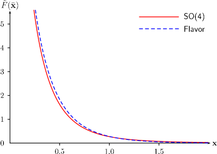
Figure 2: The diagonal flavor and $SO(4)$ form factors, in position space, for the $\ell=1$, $n=0$ spin-zero hadron.

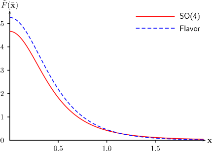
Figure 3: The diagonal flavor and $SO(4)$ form factors, in position space, for the $\ell=10$, $n=0$ spin-zero hadron.

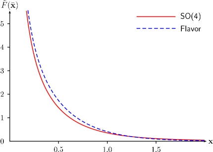
Figure 4: The diagonal flavor and $SO(4)$ form factors, in position space, for the $\ell=1$, $n=10$ spin-zero hadron.

This fact has implications for string theory. It has long been said that strings are infinite in size, because of the divergence found in $d[F(q^{2})]/d(q^{2})$ at $q^{2}=0$ for the energy-momentum form factor. However, this conclusion might be erroneous. Strings, which couple to massless gravitons, etc., might well have charge-distributions and energy-momentum distributions with power-law tails. It would be worthwhile to revisit the question of the size of strings in the light of this observation.

6.4 The structure of quarkonium

As we have seen, all of the hadrons in question appear to have a core and a power-law tail. The detailed shape of the core, though not its radial width, depends on $n$ and somewhat on $\ell$. The tail has a fixed power and a normalization which is rather insensitive to $n$ and $\ell$.

The flavor form factor tells us where the (s)quarks are located, and is insensitive to the adjoint matter. Its properties indicate that the (s)quarks are located in the core. The $SO(4)$ current, which is sensitive to the $\Phi$ fields and gluinos as well as the (s)quarks, sees a tail for any $\ell$. That this is true even for $\ell=1$ (spin-zero), for which there are no valence $\Phi$ particles in the hadron, suggests that the tail is populated by a sea of gluons, gluinos and $\Phi$ pairs. (Results from [20] suggest that the sea dominates hadrons at large $\lambda$, in contrast to expectations at small $\lambda$, where valence particles play a more significant role.) The lack of any dramatic difference between the tails of $\ell=1$ and $\ell=2$ states suggests that the valence $\Phi$ particles do not strongly change the structure of the hadron.

At large $\ell$ the $SO(4)$ form factor is independent of $\ell$, while the charge ${\cal Q}$ of the hadron is proportional to $\ell$. Raising $\ell$ by one corresponds to adding a $\Phi$ particle into the state; that this has no effect on the shape of the hadron suggests that for large $\ell$ the valence $\Phi$ particles are all coincident in position and distribution, affecting the $SO(4)$ charge distribution only through an overall scaling with $\ell$.

Increasing $n$ does change the shape of the hadron; a somewhat larger fraction of the flavor charge, $SO(4)$ charge and energy are located in central part of the core. However, even in this case the fractions of the charges located in the tail differs little between large and small $n$. It does not seem, then, that large $n$ has much impact on the basic structure of the state.

In both the large–$\ell$ and large–$n$ limits, in which the hadron mass also becomes large, the form factors have a simple structure. The core size is of order $m_{h}^{-1}$ (which is much larger than the hadron’s inverse Compton length), and the tail has a fixed normalization and power law. This suggests that the hadron acts like a bag; the $\Phi$ particles, trapped inside, have a symmetric wave function with radius of order $m_{h}^{-1}$. The puzzle, as before, is that the size of this bag is set by $1/m_{h}$, rather than the mass-scale of the $\Phi$ particles themselves.

The small size of the bag is directly tied to the deep binding of the state, in the following sense. Suppose a $\Phi$ particle’s wave function spreads out to a width $d$, where $\Lambda^{-1}\gg d\gg m_{h}$. This arrangement suffers a huge energy cost. In the stringy dual description of this phenomenon, this corresponds roughly to a part of the 7-7 string which represents the hadron descending from the D7 brane, which lies at the $AdS$ radius $L=m_{Q}\alpha^{\prime}$, down to an $AdS$ radius of order $r=\sqrt{\lambda}\alpha^{\prime}/d$, and then returning to the vicinity of the D7 brane. This would have an energy cost not of order $1/m_{h}$, as one might expect, but of order $2(m_{Q}-\sqrt{\lambda}/d)$. Thus the same physics which makes the 7-7 string nearly massless also provides a mechanism by which it can energetically trap the $\Phi$ particles. Similarly, if the $\Phi$ wavefunction remains small but moves a distance $d$ from the center of the bound state, this costs of order $2\sqrt{\lambda}m_{h}^{2}d=2(m_{Q}^{2}/\lambda)d$. This linear growth of the energy with $d$ is a less drastic effect than the previous one, but is still substantial, and is consistent with the Regge-behavior found in [10] for states of moderate spin, which are of linear size larger than $1/m_{h}$. As emphasized earlier, we still have no idea from the field theory point of view why the deep binding is present, but it is clear that the small size and deep binding are correlated.

6.5 The case of the missing form factors

Finally we turn our attention to another key observation, which was first made by Son and Stephanov [27] in the context of a recent model [13]. These authors noted that there are no anomalous magnetic form factors or quadrupole form factors for the spin-one particles in their recent model [13]. This is in contrast to hadrons in QCD, such as the $\rho$ meson [24]. The reason for this can be traced to the supergravity limit. The couplings which are required are present in the string Lagrangian but are subleading in the $\alpha^{\prime}$ expansion. The hadrons in our model also share this feature. For instance, anomalous flavor magnetic form factors $F_{m}-F_{e}$ could only be generated by a term $\alpha^{\prime}{\rm tr}F_{\mu}^{\nu}F_{\nu}^{\sigma}F_{\sigma}^{\mu}$ in the D7-brane Born-Infeld action. This term, if present, could only generate a contribution to $F_{m}-F_{e}$ which is suppressed by $1/\sqrt{\lambda}$. In a supersymmetric theory, the coefficient of this term vanishes identically. But even were supersymmetry broken at order one, so that the $F^{3}$ term had a coefficient of order one, the existence of a low-energy gravity limit would still ensure that the anomalous magnetic form factor was extremely small. The quadrupole form factors are suppressed for the same reasons. These facts should have general implications for the structure of hadrons at large ’t Hooft coupling, but we have yet to understand precisely what those might be. In particular, despite the fact that these hadrons have a nontrivial size, there is a sense in which they retain some of the properties of fundamental point particles in the large $\lambda$ limit.

6.6 Unanswered questions

There are many additional computations to consider. A key issue in these theories is to understand which aspects of hadronic physics are determined by scale invariance in the ultraviolet. Such aspects may apply approximately in QCD. We have obtained some results which probably follow from conformal invariance, possibly in combination with the large-$\lambda$ limit; it remains to prove this connection and understand which conditions are necessary and which sufficient.

The shapes and sizes of hadrons in this particular model may or may not reflect properties of typical light hadrons found in the large $\lambda$ limit; this remains to be explored. Our results presumably can be used to help interpret the structure of light hadrons purely in the ${\cal N}=4$ sector. Previously, the lack of a second scale in theories such as ${\cal N}=1^{*}$ has limited our ability both to calculate and to interpret form factors. In the present paper, we were able to separate the hadron mass scale $m_{h}$ and the confinement scale $\Lambda$, to great advantage.

On the other hand, the internal structure of these (generalized) quarkonium states still is unknown. The methods of [20] can and should be applied to them, in order to better understand what role the (s)quark and anti(s)quark are playing. It would be even more effective to study the full off-forward distribution amplitudes [16, 17, 18, 19] which can combine these pieces of information into one package.

Finally, there are a large number of still more challenging computations to do that go beyond the supergravity approximation. What happens to these (s)quark-anti(s)quark bound states when one quark mass is much larger than the other? or even when their masses have the same magnitude but different phases, which changes the interactions and the binding energies drastically? What is the structure and the dynamics governing the higher spin states? Do any of these stringier states in any way resemble their counterparts in QCD? Can we understand, perhaps even quantitatively, how states with various spins metamorphose from their small-$\lambda$ to large-$\lambda$ forms? As of now, the answers to these questions can only be guessed at, but many of them seem tractable, and there is hope that considerable progress is possible even with present-day techniques.

Appendix A Decomposition of the Form Factors

A matrix element $\langle b,p^{\prime}|J^{\mu}(q)|a,p\rangle$ can be written in terms of a sum over many hadronic states in the supergravity limit. In particular, the following decomposition of the form factor can be used:

$$\quad F_{ab}(q^{2})=\sum_{n}\frac{f_{n}g_{nab}}{q^{2}+m_{n}^{2}}$$ (114)

as illustrated in Fig. 5. This decomposition of the form factor into a sum over resonances is not justified a priori in a general confining field theory. However, in the large $N$, large $\lambda$ limit, it is exact, with corrections of order $1/N$ and $1/\sqrt{\lambda}$.

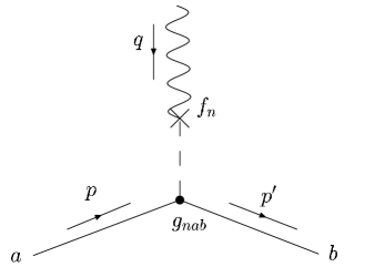
Figure 5: Decomposition of the form factor into a sum over hadron states, as in Eq. (114).

For the spin-one current matrix elements, the $f_{n}$ are the hadron decay constants of the spin-one hadrons created by the current

$${\left\langle{0}\right|}J^{\mu}(q){\left|{n,p,\epsilon}\right\rangle}=f_{n}\epsilon_{\nu}\left(\eta^{\mu\nu}-\frac{q^{\mu}q^{\nu}}{q^{2}}\right)\delta^{4}(p-q)\ ,$$

where ${\left|{0}\right\rangle}$ is the vacuum of the thoery, and ${\left|{n,p,\epsilon}\right\rangle}$ is the spin-one hadron state with mass $m_{n}$, momentum $p$ and polarization $\epsilon_{\mu}$ created by the current operator $J^{\mu}$. The $f_{n}$ are associated with the Wronksian between the normalizable and nonnormalizable mode. For instance, consider the modes created by the flavor current, which satisfy the differential equation for $\phi^{II}(\rho)$ with $\ell=0$:

$$\frac{1}{\rho^{3}}\partial(\rho^{3}\partial\phi)+\frac{m^{2}}{(1+\rho^{2})^{2}}\phi=0$$

This is already written in a self-adjoint form, so the Wronskian of two solutions is

$$W[\phi_{1},\phi_{2}]=(\phi_{1}\phi_{2}^{{}^{\prime}}-\phi_{2}\phi_{1}^{{}^{\prime}})=\frac{f}{\rho^{3}},$$ (115)

where $f$ is a constant independent of $\rho$. The fact that $f=f_{n}$ when $m=m_{n}$ follows from the form of the two-point function of the current. We may evaluate $f_{n}$ by evaluating the Wronskian at any value of $\rho$ that is convenient. We do so at $\rho\to\infty$, using the fact that the nonnormalizable mode $\phi_{non}$ associated to a conserved current goes to a $q^{2}$-independent constant as $\rho\to\infty$, while the corresponding normalizable mode $\phi_{n}$ goes as $\phi_{n}(\rho)=\xi_{n}\rho^{-2}+{\rm order}(\rho^{-3})$.

$$f_{n}=\lim_{\rho\to\infty}\rho^{3}W[\phi_{non}(m_{n}),\phi_{n}]=\phi_{non}(\rho\to\infty)\left[\rho^{3}\frac{\partial\phi_{m}}{\partial\rho}\right]_{\rho\to\infty}=-2\phi_{non}^{(0)}\xi_{n}\$$

where $\phi_{non}^{(0)}=\phi_{non}(\rho\to\infty)$. For the flavor-current case,

$$f_{n}=(-1)^{n}2(L^{2}/g_{8}R^{2})C_{0n}^{II}.$$

The $g_{nab}$ are the coupling constants between this hadron and the incoming and outgoing scalar hadrons, which are given in almost the same way as the matrix element, except that instead of a nonnormalizable mode of the gauge boson or graviton corresponding to the current, with arbitrary momentum $q^{\nu}$, we plug into the trilinear vertex a normalizable mode corresponding to the hadron $n$, on shell. For example, in the decomposition of the form factor Eq. (42), the corresponding $g_{n,n_{1},n_{2}}^{\ell}$ is given by

$$g^{\ell}_{n,n_{1},n_{2}}=g_{8}\frac{L^{2}}{2}\int_{0}^{1}dv\frac{1}{v^{2}}\phi^{II}_{0,n}(v)\phi^{I}_{\ell,n_{1}}(v)\phi^{I}_{\ell,n_{2}}(v).$$

Combining this result and the previous one with Eqs. (43) and (114), we can now compute $c^{\ell}_{n,n_{1},n_{2}}=f_{n}g^{\ell}_{n,n_{1},n_{2}}/m_{h}^{2}$.

Appendix B Some Identities

We begin with proving Eqs. (67) and (88). It’s enough to prove the following identity. Let $\zeta\equiv v+\sigma$ where $\sigma={\bf{x}}^{2}$. Then for an integer $S\geq 0$,

$${v^{S}\over\zeta^{S+1}}={(-1)^{S}\over S!}v^{S}\frac{\partial^{S}}{\partial\sigma^{S}}\frac{1}{\zeta}={1\over S!}\frac{\partial^{S}}{\partial\sigma^{S}}\left(\sigma^{S}\frac{1}{\zeta}\right)$$ (116)

where we have used the fact that $v=\zeta-\sigma$ and $S$ derivatives of $\zeta^{S-n}$, $1\leq n\leq S$, all vanish.

Let’s take the two-dimensional Fourier transform of this with respect to $d^{2}{\bf{x}}$, converting it to a function of $\bar{q}^{2}$, where $\bar{q}_{\mu}=q_{\mu}/m_{h}$ is conjugate to $x^{\mu}$. The Fourier transform of $1/\zeta$ is

$$FT\left({1\over\zeta}\right)=\frac{1}{2\pi}\int d^{2}{\bf{x}}\,e^{i\bar{q}\cdot{\bf{x}}}{1\over v+{\bf{x}}^{2}}=K_{0}(\bar{q}\sqrt{v}).$$

Now we are ready to show that Eq. (29) implies (28), and vice versa.

$$FT\left({v^{S}\over\zeta^{S+1}}\right) = {(-1)^{S}\over S!}v^{S}\frac{\partial^{S}}{\partial v^{S}}FT\left({1\over\zeta}\right)={1\over 2^{S}S!}(\bar{q}\sqrt{v})^{S}K_{S}(\bar{q}\sqrt{v})$$

$$= {(-1)^{S}\over S!}(\bar{q}^{2})^{S}{\partial^{S}\over\partial(\bar{q}^{2})^{S}}K_{0}(\bar{q}\sqrt{v})$$

This relation also follows from

$$\frac{1}{2\pi}\int d^{2}{\bf{x}}e^{i\bar{q}\cdot{\bf{x}}}{\partial^{S}\over\partial({\bf{x}}^{2})^{S}}{\bf{x}}^{2S}\tilde{F}({\bf{x}}^{2}) = \frac{1}{2\pi}\int d|{\bf{x}}|^{2}d\theta\cos(\sqrt{\bar{q}^{2}{\bf{x}}^{2}}\cos\theta){\partial^{S}\over\partial({\bf{x}}^{2})^{S}}{\bf{x}}^{2S}\tilde{F}({\bf{x}}^{2})$$ (117)

$$= \frac{1}{2}\int d|{\bf{x}}|^{2}J_{0}(\sqrt{\bar{q}^{2}{\bf{x}}^{2}}){\partial^{S}\over\partial({\bf{x}}^{2})^{S}}{\bf{x}}^{2S}\tilde{F}({\bf{x}}^{2})$$ (118)

$$= (-1)^{S}\frac{1}{2}\int d|{\bf{x}}|^{2}d\theta\left[{\partial^{S}\over\partial({\bf{x}}^{2})^{S}}J_{0}(\sqrt{\bar{q}^{2}{\bf{x}}^{2}})\right]{\bf{x}}^{2S}\tilde{F}({\bf{x}}^{2})$$ (119)

$$= (-1)^{S}\frac{1}{2}\int d|{\bf{x}}|^{2}d\theta\left({\bar{q}^{2}\over{\bf{x}}^{2}}\right)^{S}\left[{\partial^{S}\over\partial(\bar{q}^{2})^{S}}J_{0}(\sqrt{\bar{q}^{2}{\bf{x}}^{2}})\right]{\bf{x}}^{2S}\tilde{F}({\bf{x}}^{2})$$

$$= (-\bar{q}^{2})^{S}{\partial^{S}\over\partial(\bar{q}^{2})^{S}}F(\bar{q}^{2})$$

where we have used the fact that the integral is even under $\cos\theta\to-\cos\theta$, and assumed the function $F({\bf{x}}^{2})$ is sufficiently convergent at ${\bf{x}}\to 0$ and ${\bf{x}}\to\infty$ to allow the integration by parts (which is the case in our applications of this identity.)

Another useful relation that we used in derivation of Eq. (74) is

$$\frac{\partial^{n}}{\partial v^{n}}{v^{S}\over\zeta^{S+1}}={1\over S!}\frac{\partial^{S}}{\partial\sigma^{S}}\sigma^{S}\frac{\partial}{\partial v^{n}}\frac{1}{\zeta}={1\over S!}\frac{\partial^{S}}{\partial\sigma^{S}}\sigma^{S}\frac{\partial^{n}}{\partial\sigma^{n}}\frac{1}{\zeta}.$$ (121)

References

• [1] J. M. Maldacena, “The large N limit of superconformal field theories and supergravity,” Adv. Theor. Math. Phys.  2, 231 (1998) [Int. J. Theor. Phys.  38, 1113 (1999)] [arXiv:hep-th/9711200]; for a review, see O. Aharony, S. S. Gubser, J. M. Maldacena, H. Ooguri and Y. Oz, “Large N field theories, string theory and gravity,” Phys. Rept.  323, 183 (2000) [arXiv:hep-th/9905111].
• [2] C. Csaki, J. Russo, K. Sfetsos and J. Terning, “Supergravity models for 3+1 dimensional QCD,” Phys. Rev. D 60, 044001 (1999) [arXiv:hep-th/9902067].
• [3] J. Polchinski and M. J. Strassler, “The string dual of a confining four-dimensional gauge theory,” arXiv:hep-th/0003136.
• [4] I. R. Klebanov and M. J. Strassler, “Supergravity and a confining gauge theory: Duality cascades and $\chi$SB-resolution of naked singularities,” JHEP 0008, 052 (2000) [arXiv:hep-th/0007191].
• [5] O. Aharony, A. Fayyazuddin and J. M. Maldacena, “The large N limit of ${\cal N}=2,1$ field theories from three-branes in F-theory,” JHEP 9807, 013 (1998) [arXiv:hep-th/9806159]; A. Fayyazuddin and M. Spalinski, “Large N superconformal gauge theories and supergravity orientifolds,” Nucl. Phys. B 535, 219 (1998) [arXiv:hep-th/9805096].
• [6] M. Graña and J. Polchinski, “Gauge/gravity duals with holomorphic dilaton,” Phys. Rev. D 65, 126005 (2002) [arXiv:hep-th/0106014].
• [7] S. G. Naculich, H. J. Schnitzer and N. Wyllard, “Vacuum states of ${\cal N}=1^{\ast}$ mass deformations of ${\cal N}=4$ and ${\cal N}=2$ conformal gauge theories and their brane interpretations,” Nucl. Phys. B 609, 283 (2001) [arXiv:hep-th/0103047]; S. G. Naculich, H. J. Schnitzer and N. Wyllard, “A cascading ${\cal N}=1$ Sp(2N+2M) $\times$ Sp(2N) gauge theory,” Nucl. Phys. B 638, 41 (2002) [arXiv:hep-th/0204023].
• [8] A. Karch and E. Katz, “Adding flavor to AdS/CFT,” JHEP 0206, 043 (2002) [arXiv:hep-th/0205236].
• [9] A. Karch, E. Katz and N. Weiner, “Hadron masses and screening from AdS Wilson loops,” Phys. Rev. Lett.  90 (2003) 091601 [arXiv:hep-th/0211107].
• [10] M. Kruczenski, D. Mateos, R. C. Myers and D. J. Winters, “Meson spectroscopy in AdS/CFT with flavour,” JHEP 0307, 049 (2003) [arXiv:hep-th/0304032].
• [11] T. Sakai and J. Sonnenschein, “Probing flavored mesons of confining gauge theories by supergravity,” JHEP 0309, 047 (2003) [arXiv:hep-th/0305049]; J. Babington, J. Erdmenger, N. Evans, Z. Guralnik and I. Kirsch, “Chiral symmetry breaking and pions in non-supersymmetric gauge/gravity duals,” arXiv:hep-th/0306018; X.-J. Wang and S. Hu, “Intersecting branes and adding flavors to the Maldacena-Nunez background,” JHEP 0309, 017 (2003) [arXiv:hep-th/0307218]; P. Ouyang, “Holomorphic D7-branes and flavored ${\cal N}=1$ gauge theories,” arXiv:hep-th/0311084.
• [12] V. N. Gribov, “Orsay lectures on confinement. (I, II and III)” arXiv:hep-ph/9403218, arXiv:hep-ph/9404332, arXiv:hep-ph/9905285.
• [13] D. T. Son and M. A. Stephanov, “QCD and dimensional deconstruction,” arXiv:hep-ph/0304182.
• [14] See for example V. Balasubramanian, P. Kraus and A. E. Lawrence, “Bulk vs. boundary dynamics in anti-de Sitter spacetime,” Phys. Rev. D 59, 046003 (1999) [arXiv:hep-th/9805171]; W. Muck and K. S. Viswanathan, “Conformal field theory correlators from classical field theory on anti-de Sitter space. II: Vector and spinor fields,” Phys. Rev. D 58, 106006 (1998) [arXiv:hep-th/9805145]; W. Muck and K. S. Viswanathan, “The graviton in the AdS-CFT correspondence: Solution via the Dirichlet boundary value problem,” arXiv:hep-th/9810151.
• [15] J. Polchinski and M. J. Strassler, “Hard scattering and gauge/string duality,” Phys. Rev. Lett.  88, 031601 (2002) [arXiv:hep-th/0109174].
• [16] D. Muller, D. Robaschik, B. Geyer, F. M. Dittes and J. Horejsi, “Wave functions, evolution equations and evolution kernels from light-ray operators of QCD,” Fortsch. Phys.  42 (1994) 101 [arXiv:hep-ph/9812448].
• [17] X.-D. Ji, “Gauge invariant decomposition of nucleon spin,” Phys. Rev. Lett. 78, 610 (1997) [arXiv:hep-ph/9603249] .
• [18] For reviews, see A. V. Radyushkin, “Nonforward parton distributions,” Phys. Rev. D 56, 5524 (1997) [arXiv:hep-ph/9704207]; X.-D. Ji, “Off-forward parton distributions,” J. Phys. G 24, 1181 (1998) [arXiv:hep-ph/9807358].
• [19] M. Burkardt, “Impact parameter space interpretation for generalized parton distributions,” Int. J. Mod. Phys. A 18, 173 (2003) [arXiv:hep-ph/0207047].
• [20] J. Polchinski and M. J. Strassler, “Deep inelastic scattering and gauge/string duality,” JHEP 0305, 012 (2003) [arXiv:hep-th/0209211].
• [21] D. T. Son, M. A. Stephanov and M. J. Strassler, unpublished.
• [22] S. J. Brodsky and G. R. Farrar, “Scaling Laws At Large Transverse Momentum,” Phys. Rev. Lett.  31, 1153 (1973); S. J. Brodsky and G. R. Farrar, “Scaling Laws For Large Momentum Transfer Processes,” Phys. Rev. D 11, 1309 (1975).
• [23] V. A. Matveev, R. M. Muradian and A. N. Tavkhelidze, “Automodellism In The Large - Angle Elastic Scattering And Structure Of Hadrons,” Lett. Nuovo Cim.  7, 719 (1973).
• [24] B. L. Ioffe and A. V. Smilga, “Meson Widths And Form-Factors At Intermediate Momentum Transfer In Nonperturbative QCD,” Nucl. Phys. B 216, 373 (1983).
• [25] S. J. Brodsky and G. P. Lepage, “Helicity Selection Rules And Tests Of Gluon Spin In Exclusive QCD Processes,” Phys. Rev. D 24, 2848 (1981);
• [26] For a review, see V. L. Chernyak and A. R. Zhitnitsky, “Asymptotic behavior of exclusive processes in QCD,” Phys. Rept. 112, 173 (1984).
• [27] D. T. Son and M. A. Stephanov, private communication.