String Form Factors

Abstract

We compute the cross section for scattering of light string probes by randomly excited closed strings. For high energy probes, the cross section factorizes and can be used to define effective form factors for the excited targets. These form factors are well defined without the need for infinite subtractions and contain information about the shape and size of typical strings. For highly excited strings the elastic form factor can be written in terms of the ‘plasma dispersion function’, which describes charge screening in high temperature plasmas.

I Introduction

Classically, a string is a one dimensional object and its shape is simply given by the set of functions $X^{\mu}(\sigma,\tau)$. However, when we try to define the size and shape of a quantum string we run into trouble, since the coordinates $X^{\mu}$ become quantum fields on the worldsheet and, as such, undergo infinite zero-point fluctuations had . For instance, if we try to compute the mean square radius of a ground state string (i.e. a tachyon, photon or graviton, depending on the concrete string theory) we find

$${\langle}X^{2}{\rangle}\sim\alpha^{\prime}\sum_{1}^{\infty}{1\over n}=\alpha^{\prime}\log\infty\,.$$ (1)

This, however, is not the end of the story, as was recognized long ago size . The reason we get an infinite result for the mean square radius is that we are summing over the infinite modes of the string. But any real attempt to measure the size of the string will be limited by the time resolution $\epsilon$ of the experiment, and all modes with frequency $\omega>1/\epsilon$ will be averaged out and effectively cut off, so that ${\langle}X^{2}{\rangle}\sim\alpha^{\prime}\log(1/\epsilon)$.

A very natural way to measure the shape of a string is by a scattering experiment. Consider for instance the Veneziano amplitude ${\mathcal{A}}(s,t)$ describing the scattering of two open string tachyons. In the Regge limit of fixed momentum transfer $t=-q^{2}$ and high energy $E$ (with $s\sim 2E^{2}$) the amplitude can be written as gsw ; pol

$${\mathcal{A}}\sim s^{1-\alpha^{\prime}q^{2}}\Gamma(\alpha^{\prime}q^{2}-1)\,.$$ (2)

At low momentum transfer the amplitude is dominated by the photon pole in the gamma function and can be interpreted as the product of the photon propagator times the form factors ${\mathcal{F}}(q^{2})$ of the scattered strings comp :

$${\mathcal{A}}\sim{E^{2}\over q^{2}}(e^{-\alpha^{\prime}q^{2}\log E})^{2}={E^{2}\over q^{2}}{\mathcal{F}}^{2}(q^{2})\,.$$ (3)

Using the relation between form factors and mean square radius one finds

$${\langle}X^{2}{\rangle}\sim-\partial_{q^{2}}{\mathcal{F}}(q^{2})|_{q^{2}=0}\sim\alpha^{\prime}\log E\,.$$ (4)

This agrees with the previous estimate for the square radius if we relate the resolution time with the energy according to $\epsilon\sim 1/E$. The same kind of argument can be applied to the scattering of closed string tachyons. In the Regge limit, the corresponding Virasoro-Shapiro amplitude behaves like gsw ; pol

$${\mathcal{A}}_{c}\sim s^{2-{1\over 2}\alpha^{\prime}q^{2}}{\Gamma(\frac{1}{4}\alpha^{\prime}q^{2}-1)\over\Gamma(2-{1\over 4}\alpha^{\prime}q^{2})}\sim{E^{4}\over q^{2}}(e^{-\frac{1}{2}\alpha^{\prime}q^{2}\log E})^{2}={E^{4}\over q^{2}}{\mathcal{F}}_{c}^{2}(q^{2})\,,$$ (5)

giving again a mean radius that grows logarithmically with the energy.

The fact that the size of the string depends on the energy has important consequences regarding the behavior under Lorentz transformations lor (transverse spreading) and the black hole complementarity principle comp , but we shall not dwell on these interesting applications here. For us, the moral of this simple example is that defining the size and shape of strings is problematic only if we assume infinite resolution; as long as we use finite resolution probes such as other strings we get well defined, finite answers.

The same method could be used, in principle, to compute form factors for excited states, but there are many different states at every mass level and most of then are described by very complicate vertex operators. As far as we know, only for states on the leading Regge trajectory of the open string has the method been used bo . The vertex operators for these states are quite simple, and the computed form factors describe a ring distribution. This agrees with the classical interpretation of states on the leading Regge trajectory as rigidly rotating rods, with the ends describing a circumference of radius proportional to the energy.

Strings on the leading Regge trajectory are rather special, maximum angular momentum states with properties which can be very different from those of a typical excited string. Indeed, it has been recently shown that closed strings on the leading Regge trajectory have lifetimes proportional to their masses ang ; semi . There are other families of states not on the leading Regge trajectory, but still described by relatively simple vertex operators, which show an even more striking stability, with lifetimes proportional to higher powers of the mass long . Given the exponential growth of mass degeneracies, we have plenty of ground to explore and it seems likely that we can still find many surprises as we consider other families of excited states.

On the other hand, there are different contexts, such as the collapse of highly excited strings to form a black hole hor ; dam as the mass grows above the correspondence point cor , string interactions in the Boltzmann equation approach to a Hagedorn gas sal ; sen ; liz ; lowe , or the production of ‘string balls’ in a collider rob , where one is interested in general, statistical properties of typical excited strings. These general properties (typical sizes, decay and interaction rates, etc.) can be obtained by averaging over all states in a given mass level. This is the approach followed in ayr , where the averaged massless emission spectrum of highly excited strings was shown to be that of a black body at the Hagedorn temperature and in dec , where the complete decay spectrum of excited strings, including branching ratios, was computed.

In this paper we follow the last approach. Rather than studying individual excited states, we compute the equivalent of ‘unpolarized’ cross-sections, as we average over all the excited states at given mass levels of the target string, and from them extract effective form factors. In a sense, we obtain highly detailed information about the spatial distribution of excited strings by directly ‘looking’ at a statistical ensemble of them in a Rutherford type experiment. These form factors contain information not only about the geometry of excited strings, but also about their effective interactions with other strings.

This paper is organized as follows. In Section 2 we derive an exact formula for the averaged cross section corresponding to the scattering of light strings by an excited closed string and show that, for high energy probes, this result can be used to define an effective form factor for the massive string. This form factor is explicitly evaluated in Section 3 in the case of very heavy target strings, and the spatial distribution of strings of mass $M$ is investigated in detail. Section 4 considers $1/E$ corrections, where $E$ is the energy of the probe, and our conclusions and outlook are presented in Section 5.

II Averaged Cross Sections and Form Factors

We begin by computing the averaged cross section for scattering of tachyons by excited closed strings. The reason we choose closed strings is twofold. On one hand, since closed strings interact by split-join interactions that can take place anywhere along their length, the cross section contains information about the spatial distribution of the whole string; in the case of open strings, only the positions of the endpoints are mapped out. On the other hand, the computation with open strings is more involved, since one has to take into account different orderings of the vertex operators, as well as group theory factors. Similarly, we choose tachyons as probes for the sake of simplicity. As we will see, the form factors are independent of the nature of the probe, which only shows up as polarization dependent factors in the cross-section.

The averaged interaction rate is defined by averaging over all initial target states at mass level $N$ and momentum $p$ and summing over all final target states at mass level $N^{\prime}$ and momentum $p^{\prime}$. Concretely,

$${\cal R}_{c}(N,N^{\prime},k,k^{\prime})\equiv{1\over{\cal G}_{c}(N)}\sum_{\Phi_{i}|_{N}}\sum_{\Phi_{f}|_{N^{\prime}}}|{\mathcal{A}}_{c}(\Phi_{i},\Phi_{f},k,k^{\prime})|^{2}\,,$$ (6)

where the masses of the initial and final states are given by $\alpha^{\prime}M^{2}=4(N-1)$ and $\alpha^{\prime}M^{\prime 2}=4(N^{\prime}-1)$ respectively, ${\cal G}_{c}(N)$ is the degeneracy of the $N^{\mathrm{th}}$ closed string mass level, and $k$ and $k^{\prime}$ are the momenta of the incoming and outgoing tachyons. Since every closed string state can be written as the product of two open string states, it is convenient to use the well known holomorphic factorization property of 4-point tree amplitudes gsw ; pol

$${\cal A}_{c}(1,2,3,4;4\alpha^{\prime})=-\sin(2\pi\alpha^{\prime}k\cdot k^{\prime}){\cal A}_{o}(1,2,3,4;\alpha^{\prime}){\cal A}_{o}^{*}(1,3,2,4;\alpha^{\prime})\,,$$ (7)

which expresses the (unique) closed string amplitude in terms of two inequivalent cyclic orderings for the open string vertex operators. Then, given that ${\mathcal{G}}_{c}(N)={\mathcal{G}}_{o}(N)^{2}$, the averaged cross sections are related by

$${\cal R}_{c}(N,N^{\prime},k,k^{\prime};4\alpha^{\prime})=\sin^{2}(2\pi\alpha^{\prime}k\cdot k^{\prime}){\cal R}_{o}(N,N^{\prime},k,k^{\prime};\alpha^{\prime}){\cal R}_{o}(N,N^{\prime},k^{\prime},k;\alpha^{\prime})\,.$$ (8)

In what follows, we will set $\alpha^{\prime}=1/2$, which implies that our closed string rates are valid for $\alpha^{\prime}=2$.

We can use the operator formalism to write an explicit formula for ${\cal R}_{o}(N,N^{\prime},k,k^{\prime})$, extending the computations carried out in ayr ; dec for three-point functions. The details are presented in Appendix A, where it is shown that

$${\cal R}_{o}(N,N^{\prime},k,k^{\prime}) = {1\over{\cal G}_{o}(N)}\int_{0}^{1}dxx^{k\cdot p}\int_{0}^{1}dyy^{k\cdot p}\oint_{C_{w}}{dw\over w}w^{-N}f(w)^{2-D}\oint_{C_{v}}{dv\over v}v^{N-N^{\prime}}$$ (9)

$$\cdot {\langle}V_{0}(-k,1)V_{0}(-k^{\prime},y)V_{0}(k^{\prime},yv)V_{0}(k,xyv){\rangle}_{w}\,.$$

The contours $C_{w}$ and $C_{v}$ satisfy $|w|<|v|<1$ and $f(w)$ is related to the Dedekind $\eta$-function by

$$f(w)=\prod_{n=1}^{\infty}(1-w^{n})=w^{-1/24}\eta\left(\frac{\ln w}{2\pi i}\right)\,,$$ (10)

$D$ is the number of space-time dimensions and $V_{0}$ is the oscillator part of the open string tachyon vertex operator

$$V(k,z)=:e^{ik.X(z)}:=V_{0}(k,z)z^{k\cdot p-1}e^{ik\cdot x}\,.$$ (11)

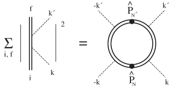
Figure 1: Averaged rate as projection of one-loop four-tachyon amplitude.

In order to evaluate (9), one should use the oscillator part of the two point correlator on the cylinder

$${\langle}V_{0}(k,z)V_{0}(k^{\prime},z^{\prime}){\rangle}_{w}=\hat{\psi}(z^{\prime}/z,w)^{\,k\cdot k^{\prime}}$$ (12)

with

$$\hat{\psi}(v,w)=(1-v)\prod_{n=1}^{\infty}{(1-w^{n}v)(1-w^{n}/v)\over(1-w^{n})^{2}}\ .$$ (13)

The $w$ and $v$ contour integrals should be done first, giving a linear combination of powers of $x$ and $y$. Then, the remaining $x$ and $y$ integrals can be written in terms of Beta functions by analytic continuation.

Note that (9) is closely related to the formula giving the 4-tachyon one-loop amplitude for the open string (see, for instance, Chapter 8 of gsw ). The main differences are in the treatment of the zero modes (there is not loop-momentum integration, the correlator involves only the oscillator parts of the vertex operators) and in the presence of contour integrals. Indeed, this formula can be understood as the projection of the usual 4-tachyon loop amplitude onto (initial) states with momentum $p$ and level $N$ and (final) states with momentum $p^{\prime}$ and level $N^{\prime}$, as shown in fig. 1.

The computation of the differential cross-section is completed by using (8), which gives the closed string rate, and adding the appropriate phase space factors and closed string coupling constant $g_{c}$

$$\Bigl{(}{d\sigma\over d\Omega}\Bigr{)}_{cm}={g_{c}^{2}\over 2E_{p}2E|v_{p}-v|}{k^{D-3}\over(2\pi)^{D-2}}{1\over 4E_{cm}}{\cal R}_{c}(N,N^{\prime},k,k^{\prime})\,,$$ (14)

where $E_{p}$ and $E$ are the initial energies of the target and probe string respectively, $v_{p}$ and $v$ are their velocities in the center of mass frame, and $E_{cm}=E_{p}+E$.

II.1 Factorization and Form Factors

Here we will show that the exact formula (9) for the interaction rate factorizes for high energy probes at fixed momentum transfer $q^{2}=(k+k^{\prime})^{2}$, allowing the definition of a form factor for the probe. We begin by noting that the Regge limit (2) of the Veneziano amplitude, which one usually obtains by using Stirling formula for the Gamma functions in

$${\mathcal{A}}(k\cdot p,k\cdot k^{\prime})={\Gamma(k\cdot p+1)\Gamma(k\cdot k^{\prime}+1)\over\Gamma(k\cdot p+k\cdot k^{\prime}+2)}=\int_{0}^{1}dxx^{k\cdot p}(1-x)^{k\cdot k^{\prime}}\,,$$ (15)

can also be obtained directly from the integral representation. In the $k\cdot p\to\infty$ limit (with fixed $k\cdot k^{\prime}$) the integral is dominated by the $x\sim 1$ region, and one can use Laplace method for integrals dominated by endpoint contributions erde . The change of variable $x=e^{-\epsilon}$ gives

$${\mathcal{A}}=\int_{0}^{\infty}d\epsilon e^{-\epsilon(k\cdot p+1)}\epsilon^{k\cdot k^{\prime}}[1+O(\epsilon)]\sim(k\cdot p)^{-k\cdot k^{\prime}-1}\Gamma(k\cdot k^{\prime}+1)[1+O\big{(}{1\over k\cdot p}\big{)}]$$ (16)

and generates an asymptotic expansion in $1/k\cdot p$. The first term of this expansion is (2) (use $k\cdot k^{\prime}+1=q^{2}/2-1$ and $-k\cdot p\sim s/2$). Note that this is quite different from the ‘hard scattering limit’ considered by Gross collaborators gross1 ; gross2 where both $k\cdot p$ and $k\cdot k^{\prime}$ are large. In that case the integral is dominated by a saddle-point in the middle of moduli space, and (2) can not be recovered from the hard scattering approximation by taking the fixed $k\cdot k^{\prime}$ limit, since the Gamma function is not reproduced.

The same kind of argument can be used with our formula for the averaged rate (9). In this case, $k\cdot p=-ME$, where $M$ is target mass and $E$ is the probe energy in the target rest frame. For $E\gg 1$ in string units and fixed $q^{2}$, the $x$ and $y$ integrals in (9) are endpoint dominated and one should be able to use Laplace method to generate an asymptotic expansion in $1/E$. To this end, make the change of variables $x=e^{-\epsilon_{1}}$, $y=e^{-\epsilon_{2}}$, and note that the leading term in the expansion corresponds to the lowest powers of $\epsilon_{1}$ and $\epsilon_{2}$. These can be easily identified by using the following OPEs

$$V_{0}(-k,1)V_{0}(-k^{\prime},y)\sim V_{0}(-q,1)\epsilon_{2}^{k\cdot k^{\prime}}+\ldots\ \ ,\ \ \ V_{0}(k^{\prime},yv)V_{0}(k,xyv)\sim V_{0}(q,v)\epsilon_{1}^{k\cdot k^{\prime}}+\ldots\ \$$ (17)

with $q=k+k^{\prime}$. Upon substitution of these OPEs in (9) we get

$${\cal R}_{o}(N,N^{\prime},k,k^{\prime}) \sim {1\over{\cal G}_{o}(N)}\int_{0}^{\infty}d\epsilon_{1}e^{-\epsilon_{1}k\cdot p}\epsilon_{1}^{k\cdot k^{\prime}}\int_{0}^{\infty}d\epsilon_{2}e^{-\epsilon_{2}k\cdot p}\epsilon_{2}^{k\cdot k^{\prime}}$$ (18)

$$\cdot \oint_{C_{w}}{dw\over w}w^{-N}f(w)^{2-D}\oint_{C_{v}}{dv\over v}v^{N-N^{\prime}}{\langle}V_{0}(-q,1)V_{0}(q,v){\rangle}_{w}\,.$$

The $1/E$ corrections to this formula come from the higher powers of $\epsilon_{1}$ and $\epsilon_{2}$ neglected in the OPEs. The $\epsilon_{1}$ and $\epsilon_{2}$ integrals can be done in terms of Gamma functions, giving

$${\cal R}_{o}(N,N^{\prime},k,k^{\prime}) \sim (EM)^{2-q^{2}}\Gamma(q^{2}/2-1)^{2}$$ (19)

$$\cdot {1\over{\cal G}_{o}(N)}\oint_{C_{w}}{dw\over w}w^{-N}f(w)^{2-D}\oint_{C_{v}}{dv\over v}v^{N-N^{\prime}}{\langle}V_{0}(-q,1)V_{0}(q,v){\rangle}_{w}.$$

This factorized form for the interaction rate suggests the following definition for the target effective form factor

$${\mathcal{F}}_{NN^{\prime}}(q^{2})={M^{-q^{2}}\over{\cal G}_{o}(N)}\oint_{C_{w}}{dw\over w}w^{-N}f(w)^{2-D}\oint_{C_{v}}{dv\over v}v^{N-N^{\prime}}{\langle}V_{0}(-q,1)V_{0}(q,v){\rangle}_{w}\,.$$ (20)

One can motivate this definition by noting that substituting (19) with (20) into (8) and using the identity $\Gamma(x)\Gamma(1-x)=\pi/\sin(\pi x)$ gives the following expression for the closed string interaction rate in the Regge limit

$${\cal R}_{c}(N,N^{\prime},k,k^{\prime})\sim M^{4}\left|{\Gamma(\frac{q^{2}}{2}-1)\over\Gamma(2-{q^{2}\over 2})}(EE^{\prime})^{1-{q^{2}\over 2}}\right|^{2}|{\mathcal{F}}_{NN^{\prime}}(q^{2})|^{2}\,.$$ (21)

For $N=N^{\prime}$ (elastic scattering) and $M\gg E$, where target recoil can be neglected ($E=E^{\prime}$), and for low momentum transfer $q^{2}\sim 0$, this gives

$${\cal R}_{c}(N,N^{\prime},k,k^{\prime})\sim\left|{(ME)^{2}\over q^{2}}{\mathcal{F}}_{c}(q^{2}){\mathcal{F}}_{NN}(q^{2})\right|^{2}$$ (22)

and we recognize the square of the Regge limit of the Virasoro-Shapiro amplitude describing tachyon-tachyon scattering (5), with one tachyon form factor ${\mathcal{F}}_{c}(q^{2})$ replaced by ${\mathcal{F}}_{NN}(q^{2})$. Thus, the effective form factor characterizes the difference between tachyon-tachyon and tachyon-probe scattering. This is analogous to the situation in field theory, where form factors ‘measure’ the departure of real particles from ideal point-like objects. Here, what we are actually measuring is the departure from being ‘tachyon–like’, or as point–like as a string can be.

It is important to note that, even though we have considered a very special limit (heavy target, elastic scattering and low momentum transfer) in order to obtain (22) and motivate our definition, the effective form factors are useful also for inelastic scattering $(N\neq N^{\prime})$ and light targets. The reason is that (21) holds as long as we are in the Regge limit of high energy probes ($E,E^{\prime}\to\infty$) and fixed (not necessarily small) momentum transfer $q^{2}$, where strings are known to interact by exchanging the leading Regge trajectory as a whole. In this sense, the effective form factors describe the coupling of the target to the leading Regge trajectory or ‘Reggeon’.

The formula for the effective form factor contains the correlator of two off-shell tachyon vertex operators. In fact (20) is essentially the off-shell extension of the tachyon emission rate for a typical open string at mass level $N$ which decays into any string at mass level $N^{\prime}$ (see eq. (2.26) of dec ). Is this related to our use of tachyons as probes? What happens if one uses other probes, such as gravitons or massive states? The only difference is that, instead of (17), one has to compute the OPEs of the corresponding vertex operators, but the tachyons still appear as the leading term (lowest power of $\epsilon_{1}$ and $\epsilon_{2}$) in the r.h.s., giving rise to the same formula for the form factor (20). In other words, the form factors describe the coupling of the target string to the leading Regge trajectory, and this is controlled by eq. (20). Using other probes just changes the coupling of the probe to the the leading Regge trajectory. This shows up as overall polarization dependent factors in (21), but the target form factor is unchanged.

One can obtain the spatial distribution of the target by Fourier transforming the elastic ($N=N^{\prime}$) form factor

$$\rho(x)={1\over(2\pi)^{D-1}}\int d^{D-1}q\,e^{iq\cdot x}{\mathcal{F}}_{NN}(q^{2})\,.$$ (23)

A first consistency check of our definition is obtained by using

$${\langle}V_{0}(-q,1)V_{0}(q,v){\rangle}_{w}=\hat{\psi}(v,w)^{-q^{2}}$$ (24)

and noting that

$${\mathcal{F}}_{NN^{\prime}}(0)=\delta_{NN^{\prime}}\,.$$ (25)

This implies that, for an experimenter which uses only very low momentum transfers ($q^{2}\sim 0$), the target will look point-like, i.e. $\rho(x)\sim\delta(x)$.

III Elastic Form Factors for heavy targets

For the rest of the paper we will study the spatial distributions of very heavy target strings and be concerned only with elastic form factors, which we write as ${\mathcal{F}}_{M}(q^{2})\equiv{\mathcal{F}}_{NN}(q^{2})$. We assume that $M$ is the largest scale in the problem, i.e. $M\gg E\gg 1$, and neglect all corrections of order $O(1/M)$. In this limit the center of mass frame coincides with the target rest frame where $E_{p}=M$, and the cross section (14) can be written as

$$\Bigl{(}{d\sigma\over d\Omega}\Bigr{)}_{cm}={g_{c}^{2}\over 16EM^{2}}{k^{D-3}\over(2\pi)^{D-2}}{\cal R}_{c}(N,N^{\prime},k,k^{\prime})\,.$$ (26)

The computation of the effective form factor (20) can be simplified by using the well known fact that, for $N\gg 1$, the $w$-integral

$$\oint_{C_{w}}{dw\over w}w^{-N}f(w)^{2-D}$$

is dominated by a saddle-point at $w\approx 1$, where the function $f(w)$ can be approximated by

$$\ln f(w)={1\over 2}\ln 2\pi-{1\over 2}\ln\beta+\frac{1}{24}\beta-\frac{\pi^{2}}{6\beta}+O\big{(}e^{-4\pi^{2}/\beta})$$ (27)

with $w\equiv e^{-\beta}$. For $w\approx 1$, $f(w)$ is a rapidly varying function, whereas the variation of the two-point correlator in the complete integral (20) is much slower. Thus the approximate position of the saddle-point can be obtained by solving $N=(D-2)\partial_{\beta}\ln f(w)$, with the result

$$\beta\approx\pi\sqrt{D-2\over 6N}={1\over 2MT_{H}}\,,$$ (28)

where $M=\sqrt{2N}$ and $T_{H}$ is the Hagedorn temperature

$$T_{H}=\frac{1}{2\pi}\sqrt{\frac{3}{D-2}}\ .$$ (29)

The solution (28) for $\beta$ is accurate up to (relative) corrections of order $O(1/M)$. We will check a posteriori that the shift in the saddle-point position due to the presence of the 2-point correlator is also of order $O(1/M)$. Thus, in the saddle-point approximation, the correlator enters only as a multiplicative correction. Taking into account that $f(w)^{2-D}$ is the partition function for the open string

$$\oint_{C_{w}}{dw\over w}w^{-N}f(w)^{2-D}={\mathcal{G}}_{o}(N)\,,$$ (30)

we arrive at the following simple formula for the elastic form factor, valid for $M\gg 1$

$${\mathcal{F}}_{M}(q^{2})=M^{-q^{2}}\oint_{C_{v}}{dv\over v}{\langle}V_{0}(-q,1)V_{0}(q,v){\rangle}_{\beta}\,,$$ (31)

where the correlator should be evaluated on a cylinder with modular parameter $w=e^{-\beta}$, with $\beta$ given by (28).

The correlator (13) is written in terms of theta functions in Appendix B, where the following explicit formula, valid for $M\gg 1$, is obtained for the elastic form factor

$${\mathcal{F}}_{M}(q^{2})=(2\pi T_{H})^{q^{2}}{\mathcal{I}}(\beta,q^{2})$$ (32)

with

$${\mathcal{I}}(\beta,q^{2})\equiv{1\over\pi}\int_{0}^{\pi}d\xi\exp\left[q^{2}\left({\xi^{2}\over 2\beta}-\ln\cosh({\pi\xi\over\beta})\right)\right]\ .$$ (33)

III.1 Evaluation of ${\mathcal{I}}(\beta,q^{2})$

The integral (33) can not be done analytically without further approximations, and these depend on the range of $q^{2}$ we are interested. For $q^{2}\gg 1/M$ ($q^{2}\gg\beta$), the change of variable $z=\pi\xi/\beta$ shows that the quadratic term in the exponent can be neglected and we are left with

$${\mathcal{I}}(\beta,q^{2})\approx{\beta\over\pi^{2}}\int_{0}^{\infty}dz\ (\cosh z)^{-q^{2}}={\beta\over 2\pi^{3/2}}{\Gamma({q^{2}\over 2})\over\Gamma({q^{2}+1\over 2})}\ \ \ ,\ \ \ q^{2}\gg{1\over M}\ .$$ (34)

Evaluating the effect of the neglected term perturbatively shows that this formula is accurate up to relative corrections of order $O(1/Mq^{2})$. One can check the consistency of the saddle-point method used to evaluate the $w$-integral at the beginning of this section by noting that $\ln{\mathcal{I}}(\beta,q^{2})$ has a logarithmic dependence on $\beta$, to be compared to the leading $1/\beta$ dependence of $\ln f(w)$ in (27).

For $q^{2}\;\raise 1.29167pt\hbox{$<$\kern-7.5pt\raise-4.73611pt\hbox{$\sim$}}\;1/M$, the quadratic term can not be neglected and (34) is no longer valid. Instead, one can use the approximation $\ln\cosh z\sim z-\ln 2$, valid for $z\gg 1$, giving

$${\mathcal{I}}(\beta,q^{2})\approx{2^{-q^{2}}\over\pi}\int_{0}^{\pi}d\xi\exp\left[-{q^{2}\over 2\beta}\,\xi(2\pi-\xi)\right]\ .$$ (35)

The relative corrections to this formula are of order $O(q^{4})$, and the approximation is valid not only for $q^{2}\;\raise 1.29167pt\hbox{$<$\kern-7.5pt\raise-4.73611pt\hbox{$\sim$}}\;1/M$, but for any $q^{2}\ll 1$. This integral can be done in terms of the ‘imaginary error function’, defined by

$$\mathrm{Erfi}(z)\equiv{2\over\sqrt{\pi}}\int_{0}^{z}dte^{t^{2}}\,.$$ (36)

The result is

$${\mathcal{I}}(\beta,q^{2})\approx{\sqrt{\pi}\over 2z}e^{-z^{2}}\mathrm{Erfi}(z)\ \ \ ,\ \ \ z\equiv{\pi q\over\sqrt{2\beta}}\ \ \ ,\ \ \ 0\leq q^{2}\ll 1\ ,$$ (37)

where we have set $2^{-q^{2}}\approx 1$. In this region one can set $(2\pi T_{H})^{q^{2}}\approx 1$ and ${\mathcal{F}}_{M}(q^{2})={\mathcal{I}}(\beta,q^{2})$. Now the dependence on $\beta$ is more involved, but one can still verify the consistency of the method used to evaluate the $w$-integral by noting that the exact equation for the saddle point is $N=(D-2)\partial_{\beta}\ln f(w)-\partial_{\beta}\ln{\mathcal{I}}(\beta,q^{2})$, with $\partial_{\beta}=-(z/2\beta)\partial_{z}$. The contribution from $\partial_{\beta}\ln{\mathcal{I}}(\beta,q^{2})$ is of order $O(1/\beta)$, and can be neglected against $\partial_{\beta}\ln f(w)$, which is of order $O(1/\beta^{2})$

It is interesting to note that (37) coincides with the function $g_{1}(q)$ describing static screening in an electron gas at high temperature.  This is related to the real part of the plasma dispersion function $\Phi(x)$ plasma by

$$g_{1}(x)={2\sqrt{\pi}\over x}\;\Phi\big{(}{x\over 4\sqrt{\pi}}\big{)}\ \ \ ,\ \ \Phi(x)=2e^{-x^{2}}\int_{0}^{x}\textrm{d}y\,e^{y^{2}}\,.$$ (38)

The coincidence may be due to the fact that $g_{1}$ is obtained from a one-loop diagram evaluated in the high temperature limit where the electron gas behaves classically, i.e. where one can use Boltzmann distribution as an approximation to Fermi-Dirac (see fet for details). Our effective form factor is obtained as an open string one-loop correlator (31) which, due to the simplifications used in the large-$M$ limit, somehow seems to go over to a (thermal) field theory one-loop correlator. On a more speculative level, this coincidence may suggest a correspondence between an ensemble of highly excited strings and a high temperature gas of particles or ‘string bits’ thorn ; brane ; halyo .

Expanding (37) around $z=0$ gives

$${\mathcal{F}}_{M}(q^{2})=\sum_{n=0}^{\infty}{(-2z^{2})^{n}\over(2n+1)!!}=1-{\pi^{2}\over 3\beta}q^{2}+O(q^{4})$$ (39)

that, using the well known relation between the power series of the form factors and the distribution moments, can be used to obtain ${\langle}r^{2n}{\rangle}$ for arbitrary $n$. In particular, the mean square radius is given by

$${\langle}r^{2}{\rangle}=-2(D-1)\partial_{q^{2}}{\mathcal{F}}(q^{2})|_{q^{2}=0}=(D-1){2\pi^{2}\over 3\beta}={4\pi^{2}\over 3}(D-1)T_{H}M\,.$$ (40)

As far as we know, the higher distribution moments have never been computed before, but the second moment was obtained long ago by Mitchell and Turok mit by oscillator methods. They found

$${\langle}r^{2}{\rangle}={D-1\over T}\sqrt{N\over 6(D-2)}\ \ \ ,\ \ \ T={1\over 2\pi\alpha^{\prime}}\ ,$$ (41)

which agrees with (40) for $\alpha^{\prime}=2$.

The ranges of validity for the two approximate expressions (34) and (37) overlap for $1/M\ll q^{2}\ll 1$. In this region, the integral is well approximated by

$${\mathcal{I}}(\beta,q^{2})\approx{1\over 2z^{2}}={\beta\over\pi^{2}q^{2}}\ \ \ ,\ \ \ 1/M\ll q^{2}\ll 1\ ,$$ (42)

which can be obtained as the $q^{2}\to 0$ limit of (34) or the $q^{2}\to\infty$ limit of (37), and has relative corrections of order $O(1/Mq^{2})$ and $O(q^{4})$. In this regime the interaction rate (21) will be proportional to $M^{2}$, giving a cross-section (26) which is totally independent of the target mass! In other words, a Rutherford type experiment designed to explore the inner structure of highly excited strings would show that this structure is independent of $M$, as long as $1/M\ll q^{2}\ll 1$. We will find a very natural interpretation for this fact below.

Lastly, for $q^{2}\gg 1$, the $q^{2}\to\infty$ limit of (34) gives

$${\mathcal{I}}(\beta,q^{2})\approx{\beta\over\sqrt{2}\pi^{3/2}q}\ \ \ ,\ \ \ q^{2}\gg 1\ .$$ (43)

To summarize, most of the structure of ${\mathcal{I}}(\beta,q^{2})$ is concentrated around $q^{2}\;\raise 1.29167pt\hbox{$<$\kern-7.5pt\raise-4.73611pt\hbox{$\sim$}}\;1/M$. Away from this region, the integral exhibits a simple power-like behavior, with a cross-over from $1/q^{2}$ to $1/q$ at the string scale $q^{2}\sim 1$ given by (34) (see fig. 2).

Figure 2: Left: ${\mathcal{I}}(\beta,q^{2})$ as a function of $z$ for $q^{2}\ll 1$ as given by (37). Right: $\log{\mathcal{I}}(\beta,q^{2})$ versus $\log q^{2}$ according to eq. (34). Note the change in slope from $-1$ to $-\frac{1}{2}$ around $q^{2}=1$.

III.2 Spatial Distribution of Heavy Strings

The spatial distribution is obtained by Fourier transforming the form factor. Since the radius of heavy strings is given by (40), and most of the interesting structure arises at low $q^{2}$, one must use (37) for the form factor. Doing the $q$-integral gives

$$\rho(r)={1\over(2\pi)^{d}}\int d^{d}q\,e^{iq\cdot r}{\mathcal{F}}_{M}(q^{2})={1\over\pi}\left({\beta\over 2\pi}\right)^{{d\over 2}}\int_{0}^{\pi}d\xi h(\xi)^{-{d\over 2}}\exp\left(-{\beta r^{2}\over 2h(\xi)}\right)\ ,$$ (44)

where $h(\xi)\equiv\xi(2\pi-\xi)$ and $d\equiv D-1$. Although $\rho(r)$ can not be evaluated analytically, it is obvious from (44) that

$$\int d^{d}x\rho(r)=1\,.$$ (45)

As the form factor describes the coupling of the string to the first Regge trajectory, and at low momentum transfer this is dominated by the graviton multiplet, we may assume that $\rho(r)$ is proportional to the mass distribution of the string. The proportionality constant is fixed by (45) and we define the mass density by $\rho_{M}(r)\equiv M\rho(r)$.

In general, $\rho_{M}(r)$ has to be computed numerically, but the behavior at ‘short distances’ $1\ll r\ll\sqrt{M}$ can be obtained by setting $h(\xi)\approx 2\pi\xi$ in  (44). The result is

$$\rho_{M}(r)\approx A_{d}r^{2-d}\ \ \ ,\ \ \ A_{d}={\pi^{-2-d/2}\over 8\,T_{H}}\,\Gamma({d\over 2}-1)$$ (46)

and we see that the inner mass distribution of the string is entirely independent of the total mass $M$. This explains the lack of dependence with $M$ in the cross section that we found after (42), which is in fact the Fourier transform of (46): The inner structure of the string is universal and independent of $M$, even at distances much larger than the string scale. Also note that the string has a rather ‘hard’ core, as exhibited by the singular behavior of $\rho_{M}$ in (46).

In the opposite limit $r\gg\sqrt{M}$ the integral in (44) is dominated by a saddle-point at $\xi=\pi$ and can be approximated by

$$\rho_{M}(r)\sim{A^{\prime}_{d}\over r}\exp(-{\beta r^{2}\over 2\pi^{2}})\,.$$ (47)

where $A^{\prime}_{d}=2^{-(d+1)/2}\pi^{-3(d-1)/2}\beta^{(d-1)/2}$.

When $r$ is neither very large nor small compared to the mean radius $R$ given by (40), $\rho_{M}(r)$ must be obtained numerically. Given the singular behavior at small $r$ given by (46), it is convenient to consider instead the radial density defined by

$${dm\over dr}=\rho_{M}(r)\Omega_{d-1}r^{d-1}\ \ \ ,\ \ \ \Omega_{d-1}={2\pi^{d/2}\over\Gamma(d/2)}\ ,$$ (48)

and the mass $m(r,M)$ within a sphere of radius $r$

$$m(r,M)=\int_{o}^{r}\textrm{d}r{dm\over dr}\,.$$ (49)

Figure 3: ${1\over M}{dm\over dr}$ (left) and $m(r,M)/M$ (right) as functions of $r/R$.

These are represented in fig. 3 for $d=25$ with $r$ in units of the mean radius $R$ and $m(r,M)$ in units of $M$. Note that the linear behavior for $dm/dr$ predicted by (46) actually holds for $r$ up to about half the mean radius. Correspondingly, we see that the inner structures of strings with masses $M$ and $2M$ coincide for $r\;\raise 1.29167pt\hbox{$<$\kern-7.5pt\raise-4.73611pt\hbox{$\sim$}}\;R/2$.

IV Low energy corrections

In this Section we will consider corrections to the factorized form (21) for the averaged interaction rate. This was obtained by using (18) as an approximation to the exact formula (9). For light targets, the exponent $k\cdot p=-ME$ in (9) is large only for $E\gg 1$, and it is obvious that the validity of the asymptotic approximation requires the use of high energy probes.

On the other hand, one might be tempted to think that, for very heavy targets, the factorization property (21) would hold even at low energies since, as long as $EM\gg 1$, the averaged rate (9) seems to be endpoint dominated even for low energy probes. In what follows we will show that this is not the case, and that (21) is the first term in an asymptotic expansion controlled by the small parameter $1/E$, not $1/EM$.

The exact formula (9) contains the $4$-point correlator

$${\langle}V_{0}(-k,1)V_{0}(-k^{\prime},y) V_{0}(k^{\prime},yv)V_{0}(k,xyv){\rangle}_{w}=$$ (50)

$$\hat{\psi}(x)^{k\cdot k^{\prime}}\hat{\psi}(xv)^{-k\cdot k^{\prime}}\hat{\psi}(xyv)^{-2}\hat{\psi}(v)^{-2}\hat{\psi}(yv)^{-k\cdot k^{\prime}}\hat{\psi}(y)^{k\cdot k^{\prime}}\,.$$

One obtains (18) by making the substitutions

$$\hat{\psi}(x)^{k\cdot k^{\prime}}\to\epsilon_{1}^{k\cdot k^{\prime}}\ \ \ ,\ \ \ \hat{\psi}(y)^{k\cdot k^{\prime}}\to\epsilon_{2}^{k\cdot k^{\prime}}$$ (51)

and setting $x=y=1$ in the other two-point functions. The corrections to (18) are obtained by expanding the correlators in powers of $\epsilon_{1}$ and $\epsilon_{2}$, and this involves differentiating the two-point function $\hat{\psi}$. Each power of $\epsilon_{1}$ or $\epsilon_{2}$ carries a factor $1/EM$ from

$$\int_{0}^{\infty}d\epsilon_{1}e^{-\epsilon_{1}k\cdot p}\epsilon_{1}^{k\cdot k^{\prime}+n}=(EM)^{1-q^{2}/2+n}\Gamma(q^{2}/2-1+n)$$ (52)

but, according to Appendix B, in the large $M$ limit

$$\hat{\psi}(v,w)\sim\frac{\beta}{\pi}\exp\left({\gamma^{2}\over 2\beta}-{\gamma\over 2}\right)\sin\left({\pi\gamma\over\beta}\right)\ ,$$ (53)

where $v\equiv e^{-\gamma}$. Thus, the $n^{\mathrm{th}}$ derivative of $\hat{\psi}$ carries a factor of $\beta^{-n}\propto M^{n}$, and the leading terms in the asymptotic expansion are powers of $1/E$. We conclude that, in general, the factorized form (21) for the interaction rate is valid only for $E\gg 1$.

This statement needs some qualifications, however, since so far we have neglected the scale set by the momentum transfer $q^{2}$. For $q^{2}\gg 1$ we have another large parameter, which has to be taken into account. In this limit one can take $k\cdot k^{\prime}\sim q^{2}/2$ and it is obvious that the leading corrections will come from $\hat{\psi}(x)^{k\cdot k^{\prime}}\hat{\psi}(xv)^{-k\cdot k^{\prime}}$ and $\hat{\psi}(yv)^{-k\cdot k^{\prime}}\hat{\psi}(y)^{k\cdot k^{\prime}}$ in (50). One should identify the terms with the highest powers of $q^{2}$ per power of $\epsilon_{1}$ or $\epsilon_{2}$. These are easily isolated by using

$$(\hat{\psi}(x)/\hat{\psi}(xv))^{q^{2}/2}\sim\left({\sin{\pi\epsilon_{1}\over\beta}\over\sin{\pi\over\beta}(\gamma+\epsilon_{1})}\right)^{q^{2}/2}\!\sim\;\left({\pi\epsilon_{1}\over\beta}\over\sin{\pi\gamma\over\beta}\right)^{q^{2}/2}\exp\bigg{[}-{q^{2}\over 2}{\pi\epsilon_{1}\over\beta}\cot{\pi\gamma\over\beta}\bigg{]}\ .$$ (54)

where we have exponentiated $(1+x)^{a}\sim e^{xa}$. Comparing this to (52), it is obvious that the resummed corrections in the $q^{2}\gg 1$ limit are equivalent to the substitution

$$k\cdot p\to k\cdot p\left(1+\frac{1}{2}{q^{2}\over k\cdot p}{\pi\over\beta}\cot{\pi\gamma\over\beta}\right)$$ (55)

which gives an overall multiplicative correction to the $\epsilon_{1}$-integral

$$(EM)^{-q^{2}/2}\to(EM)^{-q^{2}/2}\exp\left(-{1\over 4}{q^{4}\over k\cdot p}{\pi\over\beta}\cot{\pi\gamma\over\beta}\right)\ .$$ (56)

Taking into account an identical contribution from the $\epsilon_{2}$-integral and making the change of variables $\gamma=\beta/2+i\xi$ as in Appendix B, we see that instead of (33) we now have

$${\mathcal{I}}(\beta,q^{2})\to{1\over\pi}\int_{0}^{\pi}d\xi\exp\left[q^{2}\left({\xi^{2}\over 2\beta}-\ln\cosh({\pi\xi\over\beta})\right)+{i\over 2}{q^{4}\over k\cdot p}{\pi\over\beta}\tanh{\pi\xi\over\beta}\right]\ .$$ (57)

In the $q^{2}\gg 1$ limit this integral can be approximated by a gaussian, and it is easy to see that the effect of the new term in the exponent is an overall factor

$${\mathcal{I}}(\beta,q^{2})\to{\mathcal{I}}(\beta,q^{2})\exp\left(-{\pi^{2}q^{6}\over 8(k\cdot p)^{2}\beta^{2}}\right)\sim{\mathcal{I}}(\beta,q^{2})\exp\left(\!-{\pi^{2}T_{H}^{2}q^{6}\over 2E^{2}}\right)\ ,$$ (58)

where we have used $k\cdot p=-EM$ and the value of $\beta$ given by (28). Thus, for large momentum transfer it is not enough to have $E\gg 1$, and the condition on the energy becomes $E\gg q^{3}$. This implies very small scattering angles and is typical of the Regge region, modified in this case by the presence of a large mass.

V Discussion

In this paper we have used factorization and Regge limit asymptotics to obtain effective form factors for typical excited closed strings. These are written in terms of two point functions for open string tachyons on a cylinder (20) and, for very heavy targets and elastic scattering, take the simple form

$${\mathcal{F}}_{M}(q^{2})=M^{-q^{2}}\oint_{C_{v}}{dv\over v}{\langle}V_{0}(-q,1)V_{0}(q,v){\rangle}_{\beta}\,.$$ (59)

We have done this by following an old suggestion to define physically sensible string form factors by extracting them from scattering amplitudes size ; bo ; comp . This way the problem of infinite size is overcome by using light strings as finite resolution probes, which effectively cut-off the infinite sums over string modes. Moreover, the factorization process gives a well defined prescription for the off-shell correlator in (59). In this regard, we must remember that (59) is not conformally invariant, and is valid only for a particular parametrization of the world-sheet, namely the one where the two point function is given by (13).

The elastic form factor ${\mathcal{F}}_{M}(q^{2})$ has a rather simple behavior and for $q^{2}\ll 1$ can be written in closed form in terms of the ‘plasma dispersion function’ (eqs. (37) and  (38)) Since this is associated with static charge screening in a hot plasma fet , its appearance in this context is somewhat surprising, and may be related to the possibility of a ‘string bit’ interpretation for the statistical ensemble of excited strings thorn ; brane ; halyo .

Fourier transforming the formula for ${\mathcal{F}}_{M}(q^{2})$ valid for $q^{2}\ll 1$ gives the mass distribution for $r\gg 1$, i.e. at low resolution with respect to the string scale. This is shown in fig. 3, which can be considered as a ‘picture’ of the string ensemble obtained by using light string probes in a Rutherford type experiment. The fact that the interior of the string is independent of the mass indicates that, as the mass is increased, the string grows by piling up new shells on top of another, while the core is unchanged.

The form of the density $\rho(r)$ given by (44) implies the following scaling property for the mass $m(r,M)$ within a sphere of radius defined by (49)

$$m(r,M)=M\,m({r/\sqrt{M}},1)\ .$$ (60)

This kind of scaling is characteristic of random walks, and in particular implies ${\langle}r^{2}{\rangle}\propto M$. This property of the second moment is usually taken to mean that, in some sense, highly excited strings are random walks sal ; mit . The highly detailed information about the spatial distribution of excited strings obtained in this paper could be used to test this idea. In particular, one could compare the higher moments ${\langle}r^{2n}{\rangle}$, which are not uniquely determined by scaling but can be obtained from the Taylor expansion (39) of ${\mathcal{F}}_{M}(q^{2})$, to the ones predicted by some concrete realization of the random walk model.

Although we have only considered elastic scattering by heavy targets in this paper, the analysis could be extended to inelastic processes, giving information about the dynamical response of highly excited strings. One possible application is the study of thermalization in a Hagedorn gas. In particular, one could investigate how the energy of very energetic light strings gets redistributed among internal (string excitations) and external (kinetic energy) degrees of freedom after colliding with slow heavy strings.

In this paper we have studied the bosonic string for the sake of simplicity, but the technique could be extended to the superstring, although we do not expect qualitatively new results. Another question that we have omitted entirely is the effect of higher loop corrections. Since we were primarily interested in the internal structure of free excited strings, we have implicitly assumed that the coupling constant is so small that the tree level results can be trusted. Going beyond this approximation is a hard problem, but one might try something along the lines of muz ; eik . According to our analysis in Section 4, factorization holds in the Regge limit where one could try to do an eikonal resummation of leading loop effects, although this may be hampered by the fact that effective form factors, unlike ordinary amplitudes, contain no phase information.

Appendix A

Here we compute the averaged open string rate. This can be written as

$${\cal R}_{o}(N,N^{\prime},k,k^{\prime}) \equiv {1\over{\cal G}_{o}(N)}\sum_{\Phi_{i}|_{N}}\sum_{\Phi_{f}|_{N^{\prime}}}\big{|}\langle\Phi_{f}|V(k^{\prime})\Delta V(k)|\Phi_{i}\rangle\big{|}^{2}$$ (61)

$$= {1\over{\cal G}_{o}(N)}\sum_{\Phi_{i}|_{N}}\sum_{\Phi_{f}|_{N^{\prime}}}\langle\Phi_{i}|V^{\dagger}(k)\Delta V^{\dagger}(k^{\prime})|\Phi_{f}\rangle\langle\Phi_{f}|V(k^{\prime})\Delta V(k)|\Phi_{i}\rangle\,,$$

where $V$ is the tachyon vertex operator and $\Delta$ is the open string propagator

$$\Delta=\int_{0}^{1}{dx\over x}x^{L_{0}-1}\ \ \ ,\ \ \ L_{0}=\hat{N}+{p^{2}\over 2}\ .$$ (62)

Then the sums are converted into a trace with the help of the level projection operators

$$\hat{P}_{N}=\oint_{C}{dz\over z}z^{\hat{N}-N}\ \ \ ,\ \ \ \hat{N}=\sum_{n=1}^{\infty}\alpha_{-n}\cdot\alpha_{n}\ .$$ (63)

The result is

$${\cal R}_{o}(N,N^{\prime},k,k^{\prime})={1\over{\cal G}_{o}(N)}\oint_{C}{dz\over z}z^{-N}\oint_{C^{\prime}}{dz^{\prime}\over z^{\prime}}z^{\prime-N^{\prime}}{\rm Tr}\ \big{[}z^{\hat{N}}V^{\dagger}(k)\Delta V^{\dagger}(k^{\prime}){z^{\prime}}^{\hat{N}}V(k^{\prime})\Delta V(k)\big{]}$$ (64)

where $C$ and $C^{\prime}$ are small contours around the origin. Using

$$z^{L_{0}}\,V(k,1){z}^{-L_{0}}=V(k,z)\ ,\ \ \ \ \ \ z^{\hat{N}}\,V_{0}(k,1){z}^{-\hat{N}}=V_{0}(k,z)\ ,$$ (65)

where $V_{0}$ is the oscillator part of the tachyon vertex operator

$$V(k,z)=:e^{ik.X(z)}:=V_{0}(k,z)z^{k\cdot p-1}e^{ik\cdot x}$$ (66)

and making the change of variables $v=z^{\prime}$ and $w=xyzz^{\prime}$ gives

$${\cal R}_{o}(N,N^{\prime},k,k^{\prime}) = {1\over{\cal G}_{o}(N)}\int_{0}^{1}dxx^{k\cdot p}\int_{0}^{1}dyy^{k\cdot p}\oint_{C_{w}}{dw\over w}w^{-N}\oint_{C_{v}}{dv\over v}v^{N-N^{\prime}}$$ (67)

$$\cdot {\rm Tr}\ \big{[}V_{0}(-k,1)V_{0}(-k^{\prime},y)V_{0}(k^{\prime},yv)V_{0}(k,xyv)w^{\hat{N}}\big{]}\,,$$

where $p$ is the initial momentum of the target string. This can be converted into a 4-point correlator on a cylinder of modular parameter $w$ by using the identity

$${\rm Tr}\ \big{[}V_{0}(-k,1) V_{0}(-k^{\prime},y)V_{0}(k^{\prime},yv)V_{0}(k,xyv)w^{\hat{N}}\big{]}$$ (68)

$$= \;\;f(w)^{2-D}{\langle}V_{0}(-k,1)V_{0}(-k^{\prime},y)V_{0}(k^{\prime},yv)V_{0}(k,xyv){\rangle}_{w}\ ,$$

where $f(w)$ is given by (10) and $D$ is the number of space-time dimensions.

The final formula for the averaged rate is

$${\cal R}_{o}(N,N^{\prime},k,k^{\prime})={1\over{\cal G}_{o}(N)}\int_{0}^{1}dxx^{k\cdot p} \int_{0}^{1}dyy^{k\cdot p}\oint_{C_{w}}{dw\over w}w^{-N}f(w)^{2-D}\oint_{C_{v}}{dv\over v}v^{N-N^{\prime}}$$ (69)

$$\cdot {\langle}V_{0}(-k,1)V_{0}(-k^{\prime},y)V_{0}(k^{\prime},yv)V_{0}(k,xyv){\rangle}_{w}.$$

Appendix B

In order to evaluate the integral in (31) one should use (24) together with

$$\hat{\psi}(v,w)=\sqrt{v}\exp\left({-\ln^{2}v\over 2\ln w}\right)\ \psi(v,w)\,,$$ (70)

where $\psi(v,w)$ is the scalar correlator on the cylinder

$${\langle}X^{\mu}(1)X^{\nu}(v){\rangle}=-\eta^{\mu\nu}\ln\psi(v,w)$$ (71)

which is related to the Jacobi $\vartheta_{1}$ function by gsw

$$\psi(v,w)=\frac{2\pi i}{\tau}\,\frac{\vartheta_{1}(\nu|\tau)}{\vartheta^{\prime}_{1}(0|\tau)}\ \ \ ,\ \ \tau\equiv-\frac{2\pi i}{\ln w},\ \ \ ,\ \ \nu\equiv\frac{\ln v}{\ln w}\ .$$ (72)

Using the product formula for the theta function yields the following expression

$$\psi(v,w)=-\frac{2\pi}{\ln q}\sin\pi\nu\prod_{1}^{\infty}\frac{1-2q^{2n}\cos 2\pi\nu+q^{4n}}{(1-q^{2n})^{2}}\ \ \ \ ,\ \ \ q=e^{i\pi\tau}=e^{-2\pi^{2}/\beta}\ .$$ (73)

The infinite product in this formula is equal to one, up to corrections which are exponentially suppressed in the large $M$ limit. Using (70) and defining $v\equiv e^{-\gamma}$ gives

$$\hat{\psi}(v,w)\sim\frac{\beta}{\pi}\exp\left({\gamma^{2}\over 2\beta}-{\gamma\over 2}\right)\sin\left({\pi\gamma\over\beta}\right)\ .$$ (74)

We are now ready to give an explicit formula for the $v$-integral. Since $C_{v}$ can be any circle with $1>|v|>|w|$, in terms of the variable $\gamma$ the integral runs along $\gamma=c+i\xi$, where $0<c<\beta$ and $\xi$ is a real variable. Using the convenient choice $c=\beta/2$ gives

$$\oint_{C_{v}}{dv\over v}{\langle}V_{0}(-q,1)V_{0}(q,v){\rangle}_{\beta}={1\over 2\pi}\left({\beta\over\pi}\right)^{-q^{2}}e^{\beta q^{2}/8}\int_{-\pi}^{\pi}d\xi\exp\left[q^{2}\left({\xi^{2}\over 2\beta}-\ln\cosh({\pi\xi\over\beta})\right)\right]\ .$$ (75)

As we are assuming that the momentum transfer $q^{2}$ is very small compared to the mass $M$ of the target, we can set $\beta q^{2}/8\approx 0$, and using (28) one has the following simple expression for the elastic form factor

$${\mathcal{F}}_{M}(q^{2})=(2\pi T_{H})^{q^{2}}{\mathcal{I}}(\beta,q^{2})$$ (76)

where

$${\mathcal{I}}(\beta,q^{2})\equiv{1\over\pi}\int_{0}^{\pi}d\xi\exp\left[q^{2}\left({\xi^{2}\over 2\beta}-\ln\cosh({\pi\xi\over\beta})\right)\right]\ .$$ (77)

References

- (1) L. Susskind, Structure of Hadrons implied by Duality, Phys. Rev. D1 (1970) 1182.
- (2) M. Karliner, I. Klebanov and L. Susskind, Size and Shape of Strings, Int. J. Mod. Phys. A3 (1988) 1981.
- (3) M. Green, J. Schwarz and E. Witten, Superstring Theory, Vols. I and II, Cambridge 1987.
- (4) J. Polchinski, String Theory, Vols. I and II, Cambridge 1998.
- (5) L. Susskind, String Theory and the Principle of Black Hole Complementarity, Phys. Rev. Lett. 71 (1993) 2367.
- (6) L. Susskind, Strings, Black Holes and Lorentz Contraction, Phys. Rev. D49 (1994) 6606.
- (7) D. Mitchell and B. Sundborg, Measuring the Size and Shape of Strings, Nucl. Phys. B349 (1991) 159.
- (8) R. Iengo and J. G. Russo, The Decay of Massive Closed Superstrings with Maximum Angular Momentum, J. High Energy Phys. 11 (2002) 045 [hep-th/02102245].
- (9) R. Iengo and J. G. Russo, Semiclassical Decay of Strings with Maximum Angular Momentum, J. High Energy Phys. 03 (2003) 030 [hep-th/0301109].
- (10) R. Iengo and J. G. Russo, Decay of Long-Lived Closed Superstring States [hep-th/0310283].
- (11) G. T. Horowitz and J. Polchinski, Self Gravitating Fundamental Strings, Phys. Rev. D57 (1998) 2557, [hep-th/9707170].
- (12) T. Damour and G. Veneziano, Self-gravitating Fundamental Strings and Black Holes, Nucl. Phys. B568 (2000) 93 [hep-th/9907030].
- (13) G.T. Horowitz and J. Polchinsky, A Correspondence Principle for Black Holes and Strings, Phys. Rev. D55 (1997) 6189 [hep-th/9612146].
- (14) P. Salomonson and B. Skagerstam, On Superdense Superstring Gases: A Heretic String Model Approach, Nucl. Phys. B268 (1986) 349.
- (15) I. Senda, A Nucleation Model of Hadrons Based on the Dual String, Phys. Lett. B263 (1991) 270.
- (16) F.Lizzi and I. Senda, The Nucleation Model of the Hagedorn Phase Transition, Nucl. Phys. B359 (1991) 441.
- (17) D.A. Lowe and L. Thorlacius, Hot String Soup: Thermodynamics of Strings near the Hagedorn transition, Phys. Rev, D51 (1995) 665 [hep-th/9408134].
- (18) S. Dimopoulos and R. Emparan, Phys. Lett. B256 (2002) 393 [hep-ph/0108060].
- (19) D. Amati and J.G. Russo, Fundamental Strings as Black Bodies, Phys. Lett. B454 (1999) 207 [hep-th/9901092].
- (20) J. L. Mañes, Emission Spectrum of Fundamental Strings: An Algebraic Approach, Nucl. Phys. B621 (2002) 37 [hep-th/0109196].
- (21) A. Erdelyi, Asymptotic Expansions, Dover 1987.
- (22) D. J. Gross and P. F. Mende, String Theory beyond the Plank Scale, Nucl. Phys. B303 (1988) 407.
- (23) D. J. Gross and J. L. Mañes, High Energy Behavior of Open String Scattering, Nucl. Phys. B326 (1989) 73.
- (24) D. B. Fried and S. D. Conte, The Plasma Dispersion Function, Academic Press, New York 1961.
- (25) A. L. Fetter and J. D. Waleka, Quantum Theory of Many-Particle Systems, McGraw-Hill 1971.
- (26) O. Bergman and C. B. Thorn, String Bit Models for Superstring, Phys. Rev. D52 (1995) 5980 [hep-th/9506125].
- (27) E. Halyo, A. Rajaraman and L. Susskind, Braneless Black Holes, Phys. Lett. B392 (1997) 319 [hep-th/9605112].
- (28) E. Halyo, Gravitational Entropy and String Bits on Stretched Horizons [hep-th/0308166].
- (29) D. Mitchell and N. Turok, Statistical Properties of Cosmic Strings, Nucl. Phys. B294 (1987) 1138.
- (30) I. J. Muzinich and M. Soldate, High-energy Unitarity of Gravitation and Strings, Phys. Rev. D37 (1988) 359.
- (31) D. Amati, M. Ciafaloni and G. Veneziano, Classical and Quantum Gravity Effects from Planckian Energy Superstring Collisions, Int. J. Mod. Phys. A3 (1988) 1615.