Spacetime foam, CPT anomaly, and photon propagation

Abstract

The CPT anomaly of certain chiral gauge theories has been established previously for flat multiply connected spacetime manifolds $M$ of the type $\mathbb{R}^{3}\times S^{1}$, where the noncontractible loops have a minimal length. In this article, we show that the CPT anomaly also occurs for manifolds where the noncontractible loops can be arbitrarily small. Our basic calculation is performed for a flat noncompact manifold with a single “puncture,” namely $M=\mathbb{R}^{2}\times(\mathbb{R}^{2}\setminus\{0\})$. A hypothetical spacetime foam might have many such punctures (or other structures with similar effects). Assuming the multiply connected structure of the foam to be time independent, we present a simple model for photon propagation, which generalizes the single-puncture result. This model leads to a modified dispersion law of the photon. Observations of high-energy photons (gamma-rays) from explosive extragalactic events can then be used to place an upper bound on the typical length scale of these punctures.

I Introduction

Chiral gauge theories may display an anomalous breaking of Lorentz and CPT invariance if these theories are defined on a spacetime manifold $M$ with nontrivial topology K00 ; KS02 . One example of an appropriate manifold is $M=\mathbb{R}^{3}\times S^{1}$, as long as the chiral fermions have the correct boundary conditions (spin structure) over the compact space dimension. This so-called CPT anomaly has been established also for two-dimensional “chiral” $U(1)$ gauge theories over the torus $T^{2}$, where the Euclidean effective action is known exactly KN01 ; KM01 . The main points of the CPT anomaly have been reviewed in Ref. K01wigner and some background material can be found in Ref. KR03 .

The crucial ingredient of the CPT anomaly is the existence of a compact, separable space dimension with appropriate spin structure. For the case that this dimension is closed, there are corresponding noncontractible loops over the spacetime manifold, which must therefore be multiply connected. Up till now, attention has been focused on flat spacetime manifolds $M$ with topology $\mathbb{R}^{3}\times S^{1}$ or $\mathbb{R}\times T^{3}$ and with Minkowski metric $g_{\mu\nu}(x)=\eta_{\mu\nu}$ and trivial vierbeins $e_{\mu}^{a}(x)=\delta_{\mu}^{a}\,$. Here, the noncontractible loops occur at the very largest scale. But there could also be noncontractible loops from nontrivial topology at the very smallest scale, possibly related to the so-called spacetime foam W57 ; W68 ; H78 ; HPP80 ; Fetal90 ; H91 ; GH93 ; V96 . The main question is then whether or not a foam-like structure of spacetime could give rise to some kind of CPT anomaly.

In the present article we give a positive answer to this question. That is, we establish the CPT anomaly for one of the simplest possible manifolds of this type, namely $M=\mathbb{R}\times M_{3}$, where the three-dimensional space manifold $M_{3}$ is flat Euclidean space $\mathbb{R}^{3}$ with one straight line $\mathbb{R}$ removed. This particular manifold $M_{3}$ has a single “puncture” and arbitrarily small noncontractible loops.

But it is, of course, an open question whether or not spacetime really has a foam-like structure and, if so, with which characteristics. Let us just consider one possibility. Suppose that the spacetime manifold $\mathcal{M}$ is Lorentzian, $\mathcal{M}=\mathbb{R}\times\mathcal{M}_{3}$, and that the topology of $\mathcal{M}_{3}$ is multiply connected and time-independent (here, time corresponds to the coordinate $x^{0}\in\mathbb{R}$). The idea is that the multiply connectedness of $\mathcal{M}_{3}$ is “hard-wired.” The advantage of this restriction is that, for the moment, we do not have to deal with the contentious issue of topology change; cf. Refs. H91 ; V96 .

Physically, we are then interested in the long-range effects (via the CPT anomaly) of this foam-like structure of space on the propagation of light. The exact calculation of these anomalous effects is, however, not feasible for a spacetime manifold $\mathcal{M}$ with many punctures (or similar structures). We, therefore, introduce a model for the photon field over $\mathbb{R}^{4}$ which incorporates the basic features found for the case of a single puncture. The model is relatively simple and we can study the issue of photon propagation in the large-wavelength limit.

The outline of this article is as follows. In Sec. II, we establish the CPT anomaly for a flat spacetime manifold, where the spatial hypersurfaces have a single puncture corresponding to a static linear “defect.” (A similar result is obtained for a space manifold with a single wormhole, which corresponds to a static point-like defect. The details of this calculation are relegated to Appendix A.1.)

In Sec. III, we present a model for the photon field which generalizes the result of a single puncture (or wormhole). We also give a corresponding model for a real scalar field. Both models involve a “random” background field over $\mathbb{R}^{4}$, denoted by $g_{0}(x)$ for the scalar model and by $g_{1}(x)$ for the photon model. For the photon model in particular, the random background field $g_{1}(\vec{x})$ is believed to represent the effects of a static spacetime foam (a more or less realistic example for the case of permanent wormholes is given in Appendix A.2). In Sec. IV, we discuss some assumed properties of these random background fields.

In Sec. V, we calculate the dispersion laws for the scalar and photon models of Sec. III. In Sec. VI, we use observations of gamma-rays from explosive extragalactic events to place an upper bound on the typical length scale of the random background field $g_{1}(\vec{x})$ and, thereby, on the typical length scale of the postulated foam-like structure. In Sec. VII, we present some concluding remarks.

II CPT anomaly from a single defect of space

II.1 Chiral gauge theory and punctured manifold

In this section, three-space is taken to be the punctured manifold $M_{3}=\mathbb{R}\times(\mathbb{R}^{2}\setminus\{0\})=\mathbb{R}^{3}\setminus\mathbb{R}\,$. The considered three-space may be said to have a linear “defect,” just as a type-II superconductor can have a single vortex line (magnetic flux tube). The corresponding four-dimensional spacetime manifold $M=\mathbb{R}\times M_{3}$ is orientable and has Minkowski metric $(\eta_{\mu\nu})\equiv{\rm diag}(1,-1,-1,-1)$ and trivial vierbeins $e_{\mu}^{a}(x)=\delta_{\mu}^{a}\,$. This particular spacetime manifold $M$ is, of course, geodesically incomplete, but the affected geodesics constitute a set of measure zero. At the end of Sec. II.2, we briefly discuss another manifold, $N$, which is both multiply connected and geodesically complete.

The main interest here is in quantized fermion fields which propagate over the predetermined spacetime manifold $M$ and which are coupled to a given classical gauge field. We will use cylindrical coordinates around the removed line in three-space and will rewrite the four-dimensional field theory as a three-dimensional one with infinitely many fermionic fields, at least for an appropriate choice of gauge field. This procedure is analogous to the one used for the original CPT anomaly from the multiply connected manifold $\mathbb{R}^{3}\times S^{1}$.

The gauge field is written as $B_{\mu}(x)=g\,B_{\mu}^{b}(x)\,T^{b}$, with an implicit sum over $b$, where $g$ is the gauge coupling constant and the $T^{b}$ are the anti-Hermitian generators of the Lie algebra, normalized by ${\rm tr}\,(T^{b}T^{c})$ $=$ $-\,\frac{1}{2}\,\delta^{bc}$. For the matter fields, we take a single complex multiplet of left-handed Weyl fermions $\psi_{\alpha}(x)$. As a concrete case, we consider the $SO(10)$ gauge theory with left-handed Weyl fermions in the 16 representation. This particular chiral gauge theory includes, of course, the Standard Model with one family of quarks and leptons. Incidentally, the anomalous effects of this section do not occur for vectorlike theories such as Quantum Electrodynamics.

In short, the theory considered has

$$\left[\,G\,,\,R_{L}\,,\,M\,,\,e_{\mu}^{a}(x)\,\right]=\left[\,SO(10)\,,\,\mathbf{16}\,,\,\mathbb{R}^{4}\setminus\mathbb{R}^{2}\,,\,\delta^{a}_{\mu}\,\right]\,,$$ (1)

where $G$ denotes the gauge group, $R_{L}$ the representation of the left-handed Weyl fermions, $M$ the spacetime manifold, and $e_{\mu}^{a}(x)$ the vierbeins at spacetime point $x\in M$. The action for the fermionic fields reads

$$I_{\rm\,fermion}=\int_{M}\!{\rm d}^{4}x\,\,\bar{\psi}_{\dot{\alpha}}\;\delta_{a}^{\mu}\;{\rm i}\,\bar{\sigma}^{a{\dot{\alpha}}\alpha}\,\left(\partial_{\mu}+B_{\mu}\right)\,\psi_{\alpha}\,,$$ (2)

with

$$(\bar{\sigma}^{a{\dot{\alpha}}\alpha})=\left(\,\mathbf{1},-\vec{\sigma}\,\right)\,,$$ (3)

in terms of the Pauli spin matrices $\sigma^{1}$, $\sigma^{2}$, $\sigma^{3}$. Natural units with $\hbar$ $=$ $c$ $=$ $1$ are used throughout, except when stated otherwise.

Next, introduce cylindrical coordinates $(\rho,\phi,z\equiv x^{3},t\equiv x^{0})$, with

$$x^{1} \equiv\rho\cos\phi\,, x^{2} \equiv\rho\sin\phi\,,$$

$$\partial_{\rho} \equiv\cos\phi\;\partial_{1}+\sin\phi\;\partial_{2}\,, \partial_{\phi} \equiv-\rho\sin\phi\;\partial_{1}+\rho\cos\phi\;\partial_{2}\,,$$

$$\bar{\sigma}^{\rho} \equiv\cos\phi\;\bar{\sigma}^{1}+\sin\phi\;\bar{\sigma}^{2}\,, \bar{\sigma}^{\phi} \equiv-\sin\phi\;\bar{\sigma}^{1}+\cos\phi\;\bar{\sigma}^{2}\,.$$ (4)

The two spin matrices of Eq. (II.1) and $\bar{\sigma}^{z}$ are explicitly

$$(\bar{\sigma}^{\rho{\dot{\alpha}}\alpha})=\left(\begin{array}[]{cc}0&-{\rm e}^{-{\rm i}\phi}\\ -{\rm e}^{{\rm i}\phi}&0\end{array}\right),\;\;(\bar{\sigma}^{\phi{\dot{\alpha}}\alpha})=\left(\begin{array}[]{cc}0&{\rm i}\,{\rm e}^{-{\rm i}\phi}\\ -{\rm i}\,{\rm e}^{{\rm i}\phi}&0\end{array}\right),\;(\bar{\sigma}^{z{\dot{\alpha}}\alpha})=\left(\begin{array}[]{cc}-1&0\\ 0&+1\end{array}\right).$$ (5)

For the spinorial wave functions in terms of cylindrical coordinates, we take the antiperiodic boundary condition

$$\psi(\rho,\phi+2\pi,z,t)=-\psi(\rho,\phi,z,t)\,.$$ (6)

An appropriate Ansatz for the fermion fields is then

$$\psi_{\alpha}(\rho,\phi,z,t) =\sum_{n=-\infty}^{\infty}\Bigl{\{}{\rm e}^{+{\rm i}(n-1/2)\phi}\,\chi_{n}^{(+)}(\rho,z,t)\,\psi_{\alpha}^{(+)}\,\,+\,{\rm e}^{+{\rm i}(n+1/2)\phi}\,\chi_{n}^{(-)}(\rho,z,t)\,\psi_{\alpha}^{(-)}\Bigr{\}}\,,$$ (7a)

$$\bar{\psi}_{\dot{\alpha}}(\rho,\phi,z,t) =\sum_{n=-\infty}^{\infty}\Bigl{\{}{\rm e}^{-{\rm i}(n-1/2)\phi}\,\bar{\chi}_{n}^{(+)}(\rho,z,t)\,\bar{\psi}_{\dot{\alpha}}^{(+)}\,\,+\,{\rm e}^{-{\rm i}(n+1/2)\phi}\,\bar{\chi}_{n}^{(-)}(\rho,z,t)\,\bar{\psi}_{\dot{\alpha}}^{(-)}\Bigr{\}}\,,$$ (7b)

with constant spinors

$$\bigl{(}\psi^{(+)}_{\alpha}\bigr{)}=\left(\begin{array}[]{c}1\\ 0\end{array}\right)\,,\quad\bigl{(}\psi^{(-)}_{\alpha}\bigr{)}=\left(\begin{array}[]{c}0\\ 1\end{array}\right)\,,\quad\bigl{(}\bar{\psi}^{(+)}_{\dot{\alpha}}\bigr{)}=\left(\begin{array}[]{c}1\\ 0\end{array}\right)\,,\quad\bigl{(}\bar{\psi}^{(-)}_{\dot{\alpha}}\bigr{)}=\left(\begin{array}[]{c}0\\ 1\end{array}\right)\,,$$ (8)

and anticommuting fields $\chi^{(\pm)}_{n}$ which depend only on the coordinates $\rho$, $z$, and $t$. The unrestricted fields $\chi_{0}^{(\pm)}(\rho,z,t)$ and $\bar{\chi}_{0}^{(\pm)}(\rho,z,t)$ of Eqs. (7a,b) will play an important role in the next subsection.

II.2 CPT anomaly

In order to demonstrate the existence of the CPT anomaly, it suffices to consider a special class of gauge fields (denoted by a prime) which are $\phi$-independent and have vanishing components in the $\phi$ direction; cf. Ref. K00 . Specifically, we consider in this subsection the following gauge fields:

$$B^{\prime}_{\phi}=B^{\prime}_{\phi}(\rho,z,t)=0\,,\quad B^{\prime}_{m}=B^{\prime}_{m}(\rho,z,t)\,,\quad m=\rho,z,t.$$ (9)

Using the Ansatz (7) and integrating over the azimuthal angle $\phi$, the action (2) can be written as

$$I_{\rm\,fermion}= 2\pi{\rm i}\sum_{n=-\infty}^{+\infty}\,\int_{\epsilon}^{\infty}\!{\rm d}\rho\,\rho\,\int^{\infty}_{-\infty}\!{\rm d}z\,\int^{\infty}_{-\infty}\!{\rm d}t\,\,\Bigl{\{}\bar{\chi}_{n}^{(+)}\bigl{(}\,\partial_{t}+B^{\prime}_{t}\,\bigr{)}\chi_{n}^{(+)}+\bar{\chi}_{n}^{(-)}\bigl{(}\,\partial_{t}+B^{\prime}_{t}\,\bigr{)}\chi_{n}^{(-)}$$

$$-\bar{\chi}_{n}^{(+)}\bigl{(}\,\partial_{\rho}+B^{\prime}_{\rho}\,\bigr{)}\chi_{n}^{(-)}-\bar{\chi}_{n}^{(-)}\bigl{(}\,\partial_{\rho}+B^{\prime}_{\rho}\,\bigr{)}\chi_{n}^{(+)}-\bar{\chi}_{n}^{(+)}\bigl{(}\,\partial_{z}+B^{\prime}_{z}\,\bigr{)}\chi_{n}^{(+)}$$

$$+\bar{\chi}_{n}^{(-)}\bigl{(}\,\partial_{z}+B^{\prime}_{z}\,\bigr{)}\chi_{n}^{(-)}+\frac{1}{\rho}\,\Bigl{(}(n-1/2)\,\bar{\chi}_{n}^{(-)}\chi_{n}^{(+)}-(n+1/2)\,\bar{\chi}_{n}^{(+)}\chi_{n}^{(-)}\Bigr{)}\Bigr{\}}\,,$$ (10)

with $\epsilon$ a positive infinitesimal.

This action can be interpreted as a three-dimensional field theory with infinitely many Dirac fermions, labeled by $n\in\mathbb{Z}\,$. These three-dimensional Dirac fields are defined as follows:

$$\eta_{n}\equiv\left(\begin{array}[]{c}\sqrt{2\pi\rho}\>\chi_{n}^{(+)}\\ \sqrt{2\pi\rho}\>\chi_{n}^{(-)}\end{array}\right)\,,\quad\bar{\eta}_{n}\equiv\Bigl{(}\sqrt{2\pi\rho}\>\bar{\chi}_{n}^{(+)}\,,\,\sqrt{2\pi\rho}\>\bar{\chi}_{n}^{(-)}\Bigr{)}\>\gamma^{0}\,,$$ (11)

with $\gamma$-matrices

$$\gamma^{0}\equiv\sigma^{2}\,,\quad\gamma^{1}\equiv{\rm i}\,\sigma^{3}\,,\quad\gamma^{2}\equiv-{\rm i}\,\sigma^{1}\,,$$ (12)

which obey

$$\gamma^{0}\gamma^{1}\gamma^{2} = {\rm i}\,,\quad\{\gamma^{\mu},\gamma^{\nu}\}=2\,\eta^{\mu\nu}\,,$$ (13)

for $\mu,\nu=0,1,2$, and $(\eta^{\mu\nu})={\rm diag}\,(1,-1,-1)$. The action (10) is then given by

$$I_{\rm\,fermion}=\int_{\widetilde{M}_{3}}{\rm d}^{3}y\,\sum_{n=-\infty}^{+\infty}\left\{\bar{\eta}_{n}\>{\rm i}\,\gamma^{\mu}\bigl{(}\,\partial_{\mu}+\widetilde{B}^{\prime}_{\mu}\,\bigr{)}\,\eta_{n}+\frac{n}{y^{1}}\,\bar{\eta}_{n}\,\eta_{n}\right\}\,,$$ (14)

where $t$, $\rho$, $z$ have been renamed $y^{0}$, $y^{1}$, $y^{2}$, respectively, and $\widetilde{B}^{\prime}_{\mu}$ has been defined as $\widetilde{B}^{\prime}_{0}\equiv B^{\prime}_{t}$, $\widetilde{B}^{\prime}_{1}\equiv B^{\prime}_{\rho}$, $\widetilde{B}^{\prime}_{2}\equiv B^{\prime}_{z}\,$. The relevant three-dimensional spacetime manifold $\widetilde{M}_{3}=\mathbb{R}\times\mathbb{R}_{>0}\times\mathbb{R}\,$ has no boundary and is topologically equivalent to $\mathbb{R}^{3}$.

The $n=0$ sector of the theory (14) describes a massless Dirac fermion in a background gauge field, whereas the $n\neq 0$ sectors have additional position-dependent mass terms. At this moment, there is no need to specify the gauge-invariant regularization of the theory, one possibility being the use of a spacetime lattice; cf. Refs. K00 ; KS02 .

The perturbative quantum field theory based on the action (14) contains only tree and one-loop diagrams because the gauge field does not propagate and because there are no fermion self-interactions present. The effective gauge field action from the $n=0$ sector of the field theory (14) over the spacetime $\widetilde{M}_{3}$ is directly related to the effective action from charged massless Dirac fermions over $\mathbb{R}^{3}\,$.

The $n=0$ sector of the theory (14) has therefore the same “parity anomaly” as the standard $\mathbb{R}^{3}$ theory R84 ; ADM85 ; CL89 . The anomaly manifests itself in a contribution to the effective action $\Gamma[\widetilde{B}^{\prime}]$ of the form

$$\int_{\widetilde{M}_{3}}\!{\rm d}^{3}y\,\,s_{0}\,\pi\,\omega_{\mathrm{CS}}[\widetilde{B}^{\prime}_{0},\widetilde{B}^{\prime}_{1},\widetilde{B}^{\prime}_{2}]\,,$$ (15)

where $\omega_{\mathrm{CS}}$ is the Chern–Simons density

$$\omega_{\mathrm{CS}}[B_{0},B_{1},B_{2}]\equiv\frac{1}{16\pi^{2}}\,\epsilon^{\kappa\lambda\mu}\,\text{tr}\left(B_{\kappa\lambda}B_{\mu}-{\textstyle\frac{2}{3}}B_{\kappa}B_{\lambda}B_{\mu}\right)\,,$$ (16)

in terms of the Yang–Mills field strength $B_{\kappa\lambda}\equiv\partial_{\kappa}B_{\lambda}-\partial_{\lambda}B_{\kappa}+[B_{\kappa},B_{\lambda}]$, with indices running over $0,1,2$, and the Levi–Civita symbol $\epsilon^{\kappa\lambda\mu}$ normalized by $\epsilon^{012}=+1\,$. The factor $s_{0}$ in the anomalous term (15) is an odd integer which depends on the ultraviolet regularization used and we take $s_{0}=+1\,$. Note that the Chern–Simons integral (15) is a topological term, i.e., a term which is independent of the metric on $\widetilde{M}_{3}\,$. The total contribution of the $n\neq 0$ sectors to the effective action cannot be evaluated easily but is expected to lead to no further anomalies; cf. Refs. K00 ; KS02 .

The anomalous term (15) gives a contribution to the four-dimensional effective action $\Gamma[B^{\prime}]$ of the form

$$\int_{M}\!{\rm d}^{4}x\;\frac{\pi}{2\pi\rho}\,\left\{\frac{x^{1}}{\rho}\,\omega_{\mathrm{CS}}[B^{\prime}_{0},B^{\prime}_{1},B^{\prime}_{3}]+\frac{x^{2}}{\rho}\,\omega_{\mathrm{CS}}[B^{\prime}_{0},B^{\prime}_{2},B^{\prime}_{3}]\right\}\,,$$ (17)

in terms of the usual Cartesian coordinates $x^{\mu}$ and the corresponding four-dimensional gauge fields $B^{\prime}_{\mu}(x)$, $\mu=0,1,2,3$, and with the definition $\rho^{2}\equiv(x^{1})^{2}+(x^{2})^{2}$. In the form written, Eq. (17) has the same structure as the CPT anomaly term (4.1) of Ref. K00 for the $\mathbb{R}^{3}\times S^{1}$ manifold. The main properties of the anomalous term will be recalled in the next subsection.

For completeness, we mention that the CPT anomaly also occurs for another type of orientable manifold, $N=\mathbb{R}\times N_{3}\,$, which is both multiply connected and geodesically complete. This particular space manifold $N_{3}$ has a single wormhole, constructed from Euclidean three-space $\mathbb{R}^{3}$ by removing the interior of two identical balls and properly identifying their surfaces (in this case, without time shift); cf. Refs. Fetal90 ; V96 . The space “defect” is point-like if the removed balls are infinitesimally small. For an appropriate class of gauge fields $B^{\prime\prime}_{\mu}(x)$, the parity anomaly gives directly an action term analogous to Eq. (17), now over the spacetime manifold $N$ and with a dipole structure for the $\omega_{\mathrm{CS}}$ terms in the integrand. The detailed form of this anomalous term is, however, somewhat involved (see Appendix A.1) and, for the rest of this section, we return to the original manifold $M=\mathbb{R}^{4}\setminus\mathbb{R}^{2}$.

II.3 Abelian anomalous term

The gauge field $B_{\mu}(x)$ will now be restricted to the Abelian Lie subalgebra $u(1)\subset so(10)$ which corresponds to electromagnetism and the resulting real gauge field will be denoted by $A_{\mu}(x)$. In this case, the trilinear term of the Chern–Simons density (16) vanishes. For the $\phi$-independent gauge fields (9) restricted to the $u(1)$ subalgebra, the anomalous contribution (17) to the effective gauge field action $\Gamma[A^{\prime}]$ is simply

$$-\frac{1}{8\pi}\int_{M}{\rm d}^{4}x\;\epsilon^{\mu\nu\kappa\lambda}\;q^{\prime}_{\mu}\;\partial_{\nu}A^{\prime}_{\kappa}(x)\>A^{\prime}_{\lambda}(x)\,,$$ (18)

with the Levi–Civita symbol $\epsilon^{\mu\nu\kappa\lambda}$ normalized by $\epsilon^{0123}=+1$,

$$q^{\prime}_{\mu}\equiv\partial_{\mu}f^{\prime}=\frac{g^{2}}{4\pi}\;\left(0\,,\,-\frac{x^{2}}{\rho^{2}}\,,\,\frac{x^{1}}{\rho^{2}}\,,\,0\right)\,,$$ (19)

and $\rho^{2}\equiv(x^{1})^{2}+(x^{2})^{2}$.

Four remarks on the result (18) are in order. First, the action term (18), with $q^{\prime}_{\mu}\equiv\partial_{\mu}f^{\prime}$, is invariant under a four-dimensional Abelian gauge transformation, $A^{\prime}_{\mu}(x)\to A^{\prime}_{\mu}(x)+\partial_{\mu}\,\xi(x)$. Second, the Lorentz and time-reversal (T) invariances are broken (as is the CPT invariance), because the $q^{\prime}_{\mu}$ components in the effective action term (18) are fixed once and for all to the values (19); cf. Ref. K01wigner . Third, we expect no problems with unitarity and causality for the photon field, because the component $q^{\prime}_{0}$ vanishes exactly; cf. Refs. CFJ90 ; AK01 . Fourth, the overall sign of expression (18) can be changed by reversing the direction of the $z$-axis; cf.  Eq. (15).

After a partial integration, the anomalous contribution (18) can be generalized to the following term in the effective action $\Gamma[A]$:

$$\frac{1}{32\pi}\int_{\mathbb{R}^{4}}\!{\rm d}^{4}x\,\,f_{M}(x;A]\;\epsilon^{\kappa\lambda\mu\nu}\,F_{\kappa\lambda}(x)\,F_{\mu\nu}(x)\,,$$ (20)

with the field strength $F_{\mu\nu}(x)\equiv\partial_{\mu}A_{\nu}(x)-\partial_{\nu}A_{\mu}(x)$ and the integration domain extended to $\mathbb{R}^{4}$, which is possible for smooth gauge fields $A_{\mu}(x)$. (See Refs. CH85 ; N88 ; HR01 for a related discussion in the context of axion electrodynamics.) The factor $f_{M}(x;A]$ in the anomalous term (20) is both a function of the spacetime coordinates $x^{\mu}$ (on which the partial derivative $\partial_{\mu}$ acts to give $q_{\mu}$) and a gauge-invariant functional of the gauge field $A_{\mu}(x)$. This functional dependence of $f_{M}$ involves, most likely, the gauge field holonomies, defined as $h_{C}[A]\equiv\exp\left({\rm i}\oint_{C}{\rm d}x^{\mu}\,A_{\mu}(x)\right)$ for an oriented closed curve $C$; cf. Sec. 4 of Ref. K00 .

Note that the functional $f_{M}(x;A]$ in Eq. (20) is defined over $\mathbb{R}^{4}$ but carries the memory of the original (multiply connected) manifold $M$, as indicated by the suffix. [The same structure (20) has also been found for a manifold with a single static wormhole; see Appendix A.1.] Moreover, the absolute value of $f_{M}$ is of the order of the fine-structure constant,

$$\left|f_{M}(x;A]\right|=\mathrm{O}(\alpha)\,,\quad\alpha\equiv e^{2}/(4\pi)\,,$$ (21)

with the electromagnetic coupling constant $e\propto g\,$. The general expression for $f_{M}(x;A]$ is not known, but $f_{M}$ can be calculated on a case by case basis [that is, the function $f^{\prime}(x)$ for the gauge field configuration $A^{\prime}$, $f^{\prime\prime}(x)$ for $A^{\prime\prime}$, et cetera].

III Models

III.1 Motivation

The exact calculation of the CPT anomaly is prohibitively difficult for two or more punctures or wormholes. However, we expect the Abelian anomalies from the individual defects (considered in Sec. II and Appendix A.1) to add up incoherently, at least over large enough scales. We, therefore, assume that the total anomalous effect of the defects can be described by a contribution to the effective gauge field action $\Gamma[A]$ of the form (20) but with $f_{M}(x;A]$ replaced by a background field $g_{1}(x)$. This background field $g_{1}(x)$ carries the imprint of the topologically nontrivial structure of spacetime as probed by the chiral fermions. [The original spacetime manifold may, of course, have additional structure which does not contribute to the CPT anomaly and does not show up in $g_{1}(x)$.]

As discussed in the Introduction, we consider in this paper a particular type of spacetime foam for which the defects of three-space are static and have randomly distributed positions and orientations. The average distance between the defects can be assumed to be small compared to the relevant scales (set by the photon wavelength, for example) and the detailed form of $g_{1}(\vec{x})$ is not important for macroscopic considerations. We, therefore, consider $g_{1}(\vec{x})$ to be a “random” field and only assume some simple “statistical” properties. These statistical properties will be specified in Sec. IV.

It should, however, be clear that the background field $g_{1}(\vec{x})$ is not completely random. It contains, for example, the small-scale structure of the individual anomaly terms. The randomness of $g_{1}(\vec{x})$ traces back solely to the distribution of the static defects whose physical origin is unknown. In fact, the aim of the present paper is to establish and constrain some general characteristics of these hypothetical defects.

In the rest of this section, we present two concrete models with random background fields. The first model describes the propagation of a single real scalar field and the second the behavior of the photon field. Both models are defined over Minkowski spacetime, $M=\mathbb{R}^{4}$ and $g_{\mu\nu}(x)=\eta_{\mu\nu}\,$.

III.2 Real scalar field

The scalar model is defined by the action

$$I_{\mathrm{\,scalar}}= \int_{\mathbb{R}^{4}}\!{\rm d}^{4}x\,\,\,\exp\left[\,g_{0}(x)\,\right]$$

$$\times\Bigl{(}\partial_{\mu}\phi(x)\,\partial^{\mu}\phi(x)-m^{2}\phi(x)^{2}\Bigr{)}\,,$$ (22)

where $g_{0}$ is a real scalar background field of mass dimension zero. The background field $g_{0}$ is assumed to be random and further properties will be discussed in Sec. IV.

The corresponding equation of motion reads

$$(\Box+m^{2})\,\phi(x)=-\partial_{\mu}g_{0}(x)\,\partial^{\mu}\phi(x)\,,$$ (23)

with the following conventions:

$$\Box \equiv \eta^{\mu\nu}\,\partial_{\mu}\,\partial_{\nu}\,,$$

$$(\eta^{\mu\nu}) \equiv {\rm diag}(1,-1,-1,-1)\,.$$ (24)

There is no equation of motion for $g_{0}$, because $g_{0}$ is a fixed background field [the random coupling constants $g_{0}(x)$ are quenched variables]. The scalar field equation (23) will be seen to have the same basic structure as the one of the photon model in the next subsection.

For the free real scalar field $\phi^{(0)}$, we define

$$\phi^{(0)}(x) = \frac{1}{(2\pi)^{4}}\,\int\!{\rm d}^{4}k\,\,\,\widetilde{\phi}^{(0)}(k)\,{\rm e}^{-{\rm i}k\cdot x}\,,$$

$$\widetilde{\phi}^{(0)}(k) = 2\pi\,\delta(k_{\mu}k^{\mu}-m^{2})\,\bigl{[}\,\theta(k^{0})\,\widetilde{\phi}^{(0)}(\vec{k})$$ (25)

$$+\,\theta(-k^{0})\,\widetilde{\phi}^{(0)}(-\vec{k})^{*}\,\bigr{]}\,.$$

The causal Green function $\Delta(x)$ of the Klein–Gordon operator,

$$(\Box+m^{2})\,\Delta(x)=\delta^{4}(x)\,,$$ (26)

is given by

$$\Delta(x) = \frac{1}{(2\pi)^{4}}\int\!{\rm d}^{4}k\,\,\,{\rm e}^{-{\rm i}k\cdot x}\,\widetilde{\Delta}(k)\,,$$

$$\widetilde{\Delta}(k) = \frac{-1}{k^{2}-m^{2}+{\rm i}\,\epsilon}\,,$$ (27)

with the Feynman prescription for the $k^{0}$ integration contour IZ80 .

III.3 Photon field

The photon model is defined by the action

$$I_{\mathrm{\,photon}}= -\frac{1}{4}\int_{\mathbb{R}^{4}}\!{\rm d}^{4}x\,\,\Bigl{(}F_{\mu\nu}(x)F^{\mu\nu}(x)$$

$$+\,g_{1}(x)\,F_{\kappa\lambda}(x)\widetilde{F}^{\kappa\lambda}(x)\Bigr{)}\,,$$ (28)

where the Maxwell field strength tensor $F_{\mu\nu}$ and its dual $\widetilde{F}^{\kappa\lambda}$ are given by

$$F_{\mu\nu} \equiv \partial_{\mu}A_{\nu}-\partial_{\nu}A_{\mu}\,,$$

$$\widetilde{F}^{\kappa\lambda} \equiv {\textstyle\frac{1}{2}}\;\epsilon^{\kappa\lambda\mu\nu}\,F_{\mu\nu}\,,$$ (29)

with $\epsilon^{\kappa\lambda\mu\nu}$ the Levi–Civita symbol normalized by $\epsilon^{0123}=+1\,$.

The random (time-independent) background field $g_{1}$ in the action (28) is supposed to mimic the anomalous effects of a multiply connected (static) spacetime foam, generalizing the result (20) for a single puncture or wormhole. Following Eq. (21), the amplitude of the random background field $g_{1}$ is assumed to be of order $\alpha$. The typical length scale over which $g_{1}$ varies will be denoted by $l_{\rm foam}$ and further properties will be discussed in Sec. IV. Note that models of the type (28) have been considered before, but, to our knowledge, only for coupling constants varying smoothly over cosmological scales; cf. Refs. CFJ90 ; KLP02 .

The equations of motion corresponding to the action (28) are given by

$$\Box\,A^{\nu}(x)=-\partial_{\mu}g_{1}(x)\,\widetilde{F}^{\mu\nu}(x)\,,$$ (30)

provided the Lorentz gauge is used,

$$\partial^{\mu}A_{\mu}(x)=0\,.$$ (31)

The random coupling constants $g_{1}(x)$ in the action (28) are considered to be quenched variables and there is no equation of motion for $g_{1}$. As mentioned above, the basic structure of Eq. (30) equals that of Eq. (23) for the scalar model.

The general solution of the free field equation, $\Box A_{\mu}=0$, is

$$A^{(0)}_{\mu}(x) = \frac{1}{(2\pi)^{4}}\int\!{\rm d}^{4}k\,\,\widetilde{A}^{(0)}_{\mu}(k)\,{\rm e}^{-{\rm i}k\cdot x}\,,$$

$$\widetilde{A}^{(0)}_{\mu}(k) = 2\pi\,\delta(k_{\mu}k^{\mu})\,\bigl{[}\,\theta(k^{0})\,\widetilde{A}^{(0)}_{\mu}(\vec{k})$$ (32)

$$+\,\theta(-k^{0})\,\widetilde{A}^{(0)}_{\mu}(-\vec{k})^{*}\,\bigr{]}\,,$$

with

$$k^{\mu}\widetilde{A}^{(0)}_{\mu}(k)=0\,,$$ (33)

due to the gauge condition (31). The Feynman propagator IZ80 for the free field is simply $\Delta_{\mu\nu}(x)\equiv{\rm i}\,\eta_{\mu\nu}\,\Delta(x)$, with $\Delta(x)$ given by Eq. (27) for $m=0\,$.

IV Random background fields

The two models of the previous section have random background fields $g_{0}$ and $g_{1}$. For simplicity, we assume the same basic properties for these two random background fields and denote $g_{0}$ and $g_{1}$ collectively by $g$ in this section.

IV.1 General properties

The assumed properties of the background field $g(x)$ are the following:

1. $g$ is time-independent, $g=g(\vec{x})$,

2. $g$ is weak, $|g(\vec{x})|\ll 1$,

3. the average of $g(\vec{x})$ vanishes in the large volume limit,

4. $g(\vec{x})$ varies over length scales which are small compared to the considered wavelengths of the scalar field $\phi$ and photon field $A_{\mu}\,$,

5. the autocorrelation function of $g(\vec{x})$ is finite and isotropic, and drops off “fast enough” at large separations (see Secs. IV.3 and V below).

The random background field $g_{1}(\vec{x})$ for the photon case is considered to incorporate the effects of a multiply connected, static spacetime foam (cf. Sec. III.1) and assumption 5 about the lack of long-range correlations can perhaps be relaxed. Indeed, long-range correlations could arise from permanent or transient wormholes in spacetime; cf. Refs. GH93 ; V96 . But, for simplicity, we keep the five assumptions as listed above.

IV.2 Example

A specific class of random background fields $g(\vec{x})$ can be generated by superimposing copies of a localized, square-integrable shape $h(\vec{x})$ with random displacements. The displacements $\vec{x}_{n}$ are uniformly distributed over a ball of radius $R$ embedded in $\mathbb{R}^{3}$ and have average separation $a$. The number of elementary shapes is then given by $N=(4\pi/3)R^{3}/a^{3}$.

Concretely, we take

$$g_{N}(\vec{x})=\alpha\,\sum_{n=1}^{N}\epsilon_{n}\,h(\vec{x}-\vec{x}_{n})\,,$$ (34)

where the numbers $\epsilon_{n}=\pm 1$ are chosen randomly, so that $g_{N}(\vec{x})$ vanishes on average. The background field $g(\vec{x})$ is defined as the infinite volume limit,

$$g(\vec{x})=\lim_{N\to\infty}\,g_{N}(\vec{x})\,,$$ (35)

where $a$ is held constant.

The mean value and autocorrelation function of $g$ are defined by

$$\langle g\rangle\! \equiv \!\lim_{R\to\infty}\frac{1}{(4\pi/3)R^{3}}\!\int\limits_{|\vec{x}|<R}\!\!{\rm d}^{3}\vec{x}\,\,g(\vec{x})\,,$$ (36)

$$C(\vec{x})\! \equiv \!\lim_{R\to\infty}\frac{1}{(4\pi/3)R^{3}}\!\int\limits_{|\vec{y}|<R}\!\!{\rm d}^{3}\vec{y}\,\,g(\vec{y})\,g(\vec{y}+\vec{x})\,.$$ (37)

In the limit $R\to\infty$, we have perfect statistics ($N\to\infty$) and find

$$\langle g\rangle = 0\,,$$ (38)

$$C(\vec{x}) = \alpha^{2}\>a^{-3}\,\int_{\mathbb{R}^{3}}\!{\rm d}^{3}\vec{y}\,\,\,h(\vec{y})\,h(\vec{y}+\vec{x})\,.$$ (39)

The Fourier transforms of $h$ and $g_{N}$ are given by

$$\widetilde{h}(\vec{k}) = \int_{\mathbb{R}^{3}}\!{\rm d}^{3}\vec{x}\,\,{\rm e}^{-{\rm i}\vec{k}\cdot\vec{x}}\,h(\vec{x})\,,$$ (40a)

$$\widetilde{g}_{N}(\vec{k}) = \alpha\,\sum_{n=1}^{N}\epsilon_{n}\,\int_{\mathbb{R}^{3}}\!{\rm d}^{3}\vec{x}\,\,{\rm e}^{-{\rm i}\vec{k}\cdot\vec{x}}\,h(\vec{x}-\vec{x}_{n})$$ (40b)

$$= \alpha\,\sqrt{N}\;\,\widetilde{h}(\vec{k})\>\widetilde{G}_{N}(\vec{k})\,,$$

with

$$\widetilde{G}_{N}(\vec{k})\equiv\frac{1}{\sqrt{N}}\;\sum_{n=1}^{N}\epsilon_{n}\,{\rm e}^{-{\rm i}\vec{k}\cdot\vec{x}_{n}}\,.$$ (41)

The function (41) can be decomposed into an absolute value and a phase factor. The absolute value fluctuates around $1$, as follows from the expression

$$\left|\widetilde{G}_{N}(\vec{k})\right|^{2}=1+\frac{1}{N}\,\sum_{n\neq m}\epsilon_{n}\epsilon_{m}\,{\rm e}^{-{\rm i}\vec{k}\cdot(\vec{x}_{n}-\vec{x}_{m})}\,,$$ (42)

where the double sum on the right-hand side scatters around $0$. The fluctuation scale of $|\widetilde{G}_{N}(\vec{k})|$ is of order $2\pi/R$ and the same holds for the phase of $\widetilde{G}_{N}(\vec{k})$; see Fig. 1.

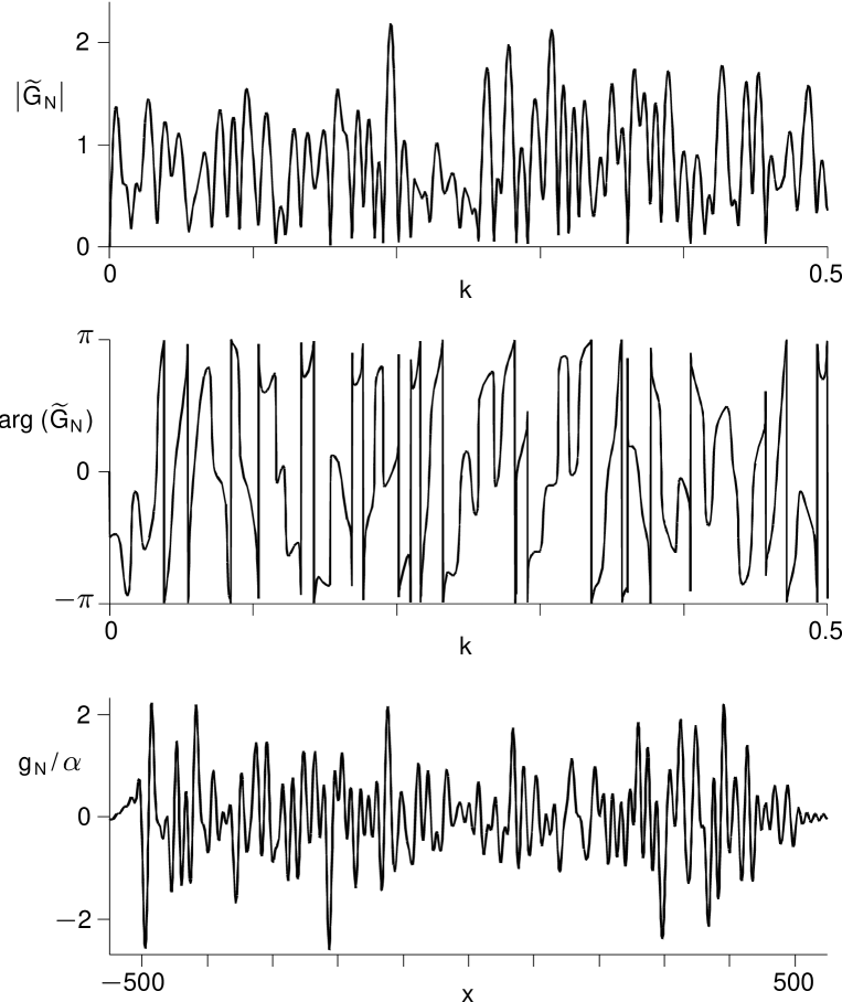
Figure 1: The top and middle panels show the momentum-space function $\widetilde{G}_{N}(k)$, defined by the one-dimensional version of Eq. (41), for $N=100$ and $R=500$. The bottom panel shows the corresponding position-space function $g_{N}(x)$, defined by the one-dimensional version of Eq. (34), for the profile function $h(x)=(20/9)\left(\,\sin\,x/2-\sin\,x/20\,\right)/x$. The Fourier transform $\widetilde{h}(k)$ of this particular profile function is nonzero and constant for $|k|\in[k_{\mathrm{low}},k_{\mathrm{high}}]$, with $k_{\mathrm{high}}=10\>k_{\mathrm{low}}>0$, and zero otherwise.

IV.3 Random phase assumption

For a given random background field $g(\vec{x})$ over $\mathbb{R}^{3}$, we define the truncated Fourier transform $\widetilde{g}_{R}(\vec{k})$ by

$$\widetilde{g}_{R}(\vec{k})\equiv\int\limits_{|\vec{x}|<R}\!{\rm d}^{3}\vec{x}\,\,{\rm e}^{-{\rm i}\vec{k}\cdot\vec{x}}\,g(\vec{x})\,,$$ (43)

with an implicit dependence on the origin of the sphere chosen. This function $\widetilde{g}_{R}$ can be parametrized as follows:

$$\widetilde{g}_{R}(\vec{k})=\sqrt{(4\pi/3)R^{3}}\,\,\widetilde{H}(\vec{k})\,\widetilde{G}_{R}(\vec{k})\,,$$ (44)

where the real function $\widetilde{H}(\vec{k})$ is obtained from the finite autocorrelation function (37),

$$C(\vec{x})=\frac{1}{(2\pi)^{3}}\int\!{\rm d}^{3}\vec{k}\,\,\,{\rm e}^{{\rm i}\vec{k}\cdot\vec{x}}\,{\widetilde{H}(\vec{k})^{2}}\,,$$ (45)

with the sign of $\widetilde{H}(\vec{k})$ chosen to make the function as smooth as possible (i.e., without cusps). Because the background field $g(\vec{x})$ is real, we have also $\widetilde{H}(-\vec{k})\>\widetilde{G}_{R}(-\vec{k})=\widetilde{H}(\vec{k})\>\widetilde{G}_{R}(\vec{k})^{*}\,$.

Motivated by the results of the preceding subsection, we assume $\widetilde{G}_{R}(\vec{k})$ to vary over momentum intervals of the order of $2\pi/R$ and $|\widetilde{G}_{R}|$ to have unit mean value. Furthermore, $\widetilde{H}(\vec{k})^{2}$ is taken to be smooth on scales of the order of $2\pi/R$, provided $R$ is large enough. For the isotropic case $\widetilde{H}(\vec{k})=\widetilde{H}(k)$, with $k\equiv|\vec{k}|$, and large enough $R$, we explicitly assume the inequality

$$\left|\,\int_{0}^{\infty}\!{\rm d}k\,\,\cos(kR)\,\widetilde{H}(k)^{2}\,\right|\ll\int_{0}^{\infty}\!{\rm d}k\,\,\widetilde{H}(k)^{2}\,,$$ (46)

with a finite positive number on the right-hand side.

Now suppose that we have to evaluate a double integral of the form

$$\int\!{\rm d}^{3}\vec{k}\,\,\!\int\!{\rm d}^{3}\vec{p}\,\,f(\vec{p},\vec{k})\,\widetilde{G}_{R}(\vec{k})\,\widetilde{G}_{R}(\vec{p})\,,$$ (47)

where $f$ is a function which is approximately constant over momentum intervals of the order of $2\pi/R\,$. Due to the rapid phase oscillations of $\widetilde{G}_{R}$, a significant contribution can arise only for $\vec{k}\approx-\vec{p}\,$ and $\widetilde{G}_{R}(\vec{k})\,\widetilde{G}_{R}(\vec{p})$ can effectively be replaced by a smeared delta-function.

The specific form of this smeared delta-function does not matter in the limit $R\to\infty$ and we simply choose

$$\delta_{R}^{3}(\vec{k})\equiv\prod_{j=1}^{3}\,\frac{\sin(k_{j}R)}{\pi k_{j}}\;.$$ (48)

We then have the result

$$\int\!{\rm d}^{3}\vec{k}\,\,\!\int\!{\rm d}^{3}\vec{p}\,\,f(\vec{p},\vec{k})\,\widetilde{G}_{R}(\vec{k})\,\widetilde{G}_{R}(\vec{p})$$

$$\approx{\cal N}\,\int\!{\rm d}^{3}\vec{k}\,\,\!\int\!{\rm d}^{3}\vec{p}\,\,f(\vec{p},\vec{k})\,\delta_{R}^{3}(\vec{k}+\vec{p})\,,$$ (49)

with a normalization factor $\cal N$ to be determined shortly. On the right-hand side of Eq. (49), the absolute values of $\widetilde{G}_{R}$ have been replaced by their average value $1$, since $f(\vec{p},\vec{k})$ is assumed to be slowly varying.

In order to determine the normalization factor $\cal N$, reconsider the autocorrelation function (37). Using Eqs. (44) and (48), the autocorrelation function can be written as follows:

$$C(\vec{x})= \lim_{R\to\infty}\frac{1}{(2\pi)^{3}}\int\!{\rm d}^{3}\vec{k}\,\,\!{\rm d}^{3}\vec{p}\,\,\,\delta^{3}_{R}(\vec{k}+\vec{p})\,\,{\rm e}^{{\rm i}\vec{p}\cdot\vec{x}}$$

$$\times\widetilde{H}(\vec{k})\,\widetilde{H}(\vec{p})\,\,\widetilde{G}_{R}(\vec{k})\,\widetilde{G}_{R}(\vec{p})\,.$$ (50)

Since there is already a delta-function present in the integrand of (50), the product $\widetilde{G}_{R}(\vec{k})\,\widetilde{G}_{R}(\vec{p})$ can simply be replaced by ${\cal N}\,\delta_{R}^{3}(\vec{k}+\vec{p})$, which gives the correct behavior for $\vec{k}\approx-\vec{p}\,$. With

$$\delta^{3}_{R}(\vec{k}+\vec{p})\,\delta^{3}_{R}(\vec{k}+\vec{p})\to\frac{R^{3}}{\pi^{3}}\,\,\delta^{3}(\vec{k}+\vec{p})\,,$$ (51)

for $R\to\infty$, Eqs. (45) and (50) are consistent if

$${\cal N}=(\pi/R)^{3}\,.$$ (52)

This fixes the normalization factor $\cal N$ of Eq. (49), which will be used extensively in the next section.

V Dispersion laws

V.1 Scalar model

We first turn to the scalar model (22), as a preliminary for the calculation of the photon model in the next subsection. In order to have a well defined Fourier transform of $g_{0}$, the system is put inside a sphere of radius $R$ with free boundary conditions for the real scalar field $\phi$. In momentum space, the scalar field equation (23) becomes

$$(k^{2}-m^{2})\,\widetilde{\phi}(k)=-\frac{1}{(2\pi)^{4}}\int\!{\rm d}^{4}q\,\,\widetilde{g}_{0R}(q)\,q_{\mu}\,(k^{\mu}-q^{\mu})\,\widetilde{\phi}(k-q)\,.$$ (53)

According to Eq. (44), the momentum-space function $\widetilde{g}_{0R}$ has the form

$$\widetilde{g}_{0R}(k)\equiv 2\pi\delta(k^{0})\,\sqrt{(4\pi/3)\,R^{3}}\,\,\widetilde{H}_{0}(|\vec{k}|)\,\widetilde{G}_{0R}(\vec{k})\,,$$ (54)

where $\widetilde{G}_{0R}$ is assumed to have the statistics properties discussed in Sec. IV.3. Furthermore, we have assumed isotropy of $\widetilde{H}_{0}$; see Sec. IV.1.

We will now show that the main effect of the random background field $g_{0}(\vec{x})$ can be expressed in the form of a modified dispersion law for the scalar modes, at least for large enough wavelengths. The basic idea is to expand the solution of Eq. (53) perturbatively to second order in $g_{0}$ (there is no contribution at first order) and to compare it with the first-order solution of a modified field equation,

$$(k^{2}-m^{2})\,\widetilde{\phi}(k)=A\bigl{(}|\vec{k}|\bigr{)}\;\widetilde{\phi}(k)\,.$$ (55)

The dispersion law will then be given by

$$\omega^{2}=m^{2}+|\vec{k}|^{2}+A\bigl{(}|\vec{k}|\bigr{)}\,,$$ (56)

with $A$ expressed in terms of the random background field $g_{0}(\vec{x})$.

In the limit $R\to\infty$, the perturbative second-order contribution to $\widetilde{\phi}(k)$ reads

$$\widetilde{\phi}^{(2)}(k)= \lim_{R\to\infty}\,\frac{1}{(2\pi)^{8}}\>\widetilde{\Delta}(k)\int\!{\rm d}^{4}q\,\,\widetilde{g}_{0R}(q)\,\,q_{\mu}\,(k-q)^{\mu}\,\widetilde{\Delta}(k-q)$$

$$\times\int\!{\rm d}^{4}p\,\,\widetilde{g}_{0R}(k-p-q)\,\,(k-p-q)_{\nu}\>p^{\nu}\,\widetilde{\phi}^{(0)}(p)$$

$$= -\lim_{R\to\infty}\,\widetilde{\Delta}(k)\,\frac{(4\pi/3)R^{3}}{(2\pi)^{6}}\,\int\!{\rm d}^{3}\vec{q}\,\,\int\!{\rm d}^{3}\vec{p}\,\,\,\widetilde{H}_{0}(|\vec{q}|)\,\,\widetilde{H}_{0}(|\vec{k}-\vec{p}-\vec{q}|)\,\,\widetilde{G}_{0R}(\vec{q})\,$$

$$\times\,\widetilde{G}_{0R}(\vec{k}-\vec{p}-\vec{q})\,\,\widetilde{\Delta}(k^{0},\vec{k}-\vec{q})\left(\vec{q}\cdot(\vec{q}-\vec{k})\right)\left((\vec{k}-\vec{p}-\vec{q})\cdot\vec{p}\,\right)\,\widetilde{\phi}^{(0)}(k^{0},\vec{p})\,,$$ (57)

where Eq. (54) has been used. According to Eqs. (49) and (52), we can replace the product $\widetilde{G}_{0R}\,\widetilde{G}_{0R}$ by $(\pi/R)^{3}\,\delta^{3}_{R}$ and take the limit $R\to\infty$,

$$\widetilde{\phi}^{(2)}(k) =\frac{1}{12\,(2\pi)^{2}}\;\widetilde{\Delta}(k)\>\int\!{\rm d}^{3}\vec{q}\,\,\,\widetilde{H}_{0}(|\vec{q}|)^{2}\,\widetilde{\Delta}(k^{0},\vec{k}-\vec{q})\,\left(\vec{q}\cdot(\vec{q}-\vec{k})\right)\left(\vec{q}\cdot\vec{k}\,\right)\,\widetilde{\phi}^{(0)}(k)\,.$$ (58)

At the given perturbative order, $k_{\mu}k^{\mu}-m^{2}$ can be put to zero in the integrand of Eq. (58), because of the delta-function contained in the free field $\widetilde{\phi}_{0}(k)$ of Eq. (25). By comparison with the first order solution of Eq. (55), the operator $A$ is identified as

$$A\bigl{(}|\vec{k}|\bigr{)}=\frac{1}{12\,(2\pi)^{2}}\,\int\!{\rm d}^{3}\vec{q}\,\,\,\widetilde{H}_{0}(|\vec{q}|)^{2}\;\frac{\bigl{(}\vec{q}\cdot(\vec{q}-\vec{k})\bigr{)}\bigl{(}\vec{q}\cdot\vec{k}\,\bigr{)}}{2\vec{k}\cdot\vec{q}-|\vec{q}|^{2}+{\rm i}\,\epsilon}\,.$$ (59)

Following the discussion of Sec. IV.1, we now assume that $\widetilde{H}_{0}(|\vec{q}|)$ vanishes for momenta $|\vec{q}|<q_{\rm low}$ (cf. Fig. 1) and that $|\vec{k}|<q_{\rm low}/2$. Performing the angular integrals in Eq. (59), one finds

$$A\bigl{(}|\vec{k}|\bigr{)}=\frac{1}{24\pi}\,\int_{0}^{\infty}\!{\rm d}q\,\,q^{2}\,\widetilde{H}_{0}(q)^{2}\left(\frac{1}{2}\,q^{2}+\frac{q^{3}}{8|\vec{k}|}\>\ln\left|\frac{q-2|\vec{k}|}{q+2|\vec{k}|}\right|\,\right)\,,$$ (60)

where the lower limit of the integral is effectively $q_{\rm low}$. Because of the large-wavelength assumption $|\vec{k}|<q_{\rm low}/2$, the same result is obtained if the causal Green function $\widetilde{\Delta}$ in the first integral of Eq. (57) is replaced by, for example, the retarded or the advanced Green function.

Next, the logarithm of Eq. (60) is expanded in terms of $|\vec{k}|/q$, which gives

$$A\bigl{(}|\vec{k}|\bigr{)}=\frac{1}{24\pi}\,\int_{0}^{\infty}\!{\rm d}q\,\,\,\widetilde{H}_{0}(q)^{2}\left(-\frac{2}{3}\,q^{2}\,|\vec{k}|^{2}-\frac{8}{5}\,|\vec{k}|^{4}\right)+\mathrm{O}\left(|\vec{k}|^{6}/q_{\rm low}^{4}\right)\,.$$ (61)

This result can also be written as

$$A\bigl{(}|\vec{k}|\bigr{)}=-\frac{\pi}{18}\,C_{0}(0)\,|\vec{k}|^{2}-\frac{2\pi}{15}\left(\,\int_{0}^{\infty}\!{\rm d}x\,\,x\,C_{0}(x)\right)|\vec{k}|^{4}+\mathrm{O}\left(|\vec{k}|^{6}/q_{\rm low}^{4}\right)\,,$$ (62)

in terms of the autocorrelation function (45), which is isotropic because $\widetilde{H}_{0}$ is,

$$C_{0}=C_{0}\bigl{(}|\vec{x}|\bigr{)}=\frac{2}{(2\pi)^{2}}\,\int_{0}^{\infty}\!{\rm d}q\,\,q^{2}\;\frac{\sin\,q|\vec{x}|}{q|\vec{x}|}\;\widetilde{H}_{0}(q)^{2}\,.$$ (63)

In order to make the identification of the $|\vec{k}|^{4}$ prefactor in Eq. (62), it has been assumed that the behavior of $\widetilde{H}_{0}(q)^{2}$ is sufficiently smooth; cf. Eq. (46).

From Eqs. (56) and (62), the dispersion law of the scalar is

$$\omega^{2}=m^{2}\,+(1-a_{0})\,|\vec{k}|^{2}\,-b_{0}\,|\vec{k}|^{4}\,+\,\dots\,,$$ (64)

where the dots stand for higher order contributions and the positive coefficients $a_{0}$ and $b_{0}$ are given by

$$a_{0}\equiv\frac{\pi}{18}\,C_{0}(0)\,,\quad b_{0}\equiv\frac{2\pi}{15}\int_{0}^{\infty}\!{\rm d}x\,\,x\,C_{0}(x)\,.$$ (65)

The isotropic autocorrelation function $C_{0}(x)$ is defined by Eq. (37) with $g$ replaced by the random background field $g_{0}$ from the action (22).

The main purpose of the scalar calculation is to prepare the way for the photon calculation in the next subsection, but let us comment briefly on the result found. Setting the scalar mass $m$ to zero in the action (22), our calculation gives no additional mass term in the dispersion law (64). It is, however, not clear what the random background field $g_{0}$ of the model (22) really has to do with a (static) spacetime foam. The propagation of an initially massless scalar could very well be strongly modified in a genuine spacetime foam; cf. Ref. HPP80 .

V.2 Photon model

To obtain the dispersion law for the photon model (28), we proceed along the same lines as for the scalar case. Again, the system is put inside a sphere of radius $R$, so that the truncated Fourier transform $\widetilde{g}_{1R}$ occurs in the momentum-space field equation,

$$k^{2}\widetilde{A}^{\nu}(k)=-\frac{1}{(2\pi)^{4}}\,\int\!{\rm d}^{4}q\,\,\widetilde{g}_{1R}(q)\,\epsilon^{\mu\nu\kappa\lambda}\,q_{\mu}\,(k-q)_{\kappa}\,\widetilde{A}_{\lambda}(k-q)\,.$$ (66)

For this truncated background field $\widetilde{g}_{1R}$, we assume a form analogous to Eq. (54),

$$\widetilde{g}_{1R}(k)\equiv 2\pi\delta(k^{0})\,\sqrt{(4\pi/3)\,R^{3}}\,\,\widetilde{H}_{1}(|\vec{k}|)\,\widetilde{G}_{1R}(\vec{k})\,,$$ (67)

where $\widetilde{G}_{1R}$ is a random function of the type discussed in Sec. IV.3.

The second-order contribution to the perturbative solution of Eq. (66) is given by

$$\widetilde{A}^{(2)\nu}(k) =\lim_{R\to\infty}\,\frac{1}{(2\pi)^{8}}\,\widetilde{\Delta}(k)\,\int\!{\rm d}^{4}q\,\,\widetilde{g}_{1R}(q)\,\epsilon^{\mu\nu\kappa\lambda}\,q_{\mu}\,(k-q)_{\kappa}\,\,\widetilde{\Delta}(k-q)$$

$$\quad\times\,\int\!{\rm d}^{4}p\,\,\,\widetilde{g}_{1R}(k-p-q)\,\epsilon_{\alpha\beta\gamma\lambda}\,(k-p-q)^{\alpha}\,p^{\beta}\,\widetilde{A}^{(0)\gamma}(p)\,.$$ (68)

Using Eq. (67) and replacing the product $\widetilde{G}_{1R}\,\widetilde{G}_{1R}$ by $(\pi/R)^{3}\,\delta^{3}_{R}\,$, one finds in the limit $R\to\infty$:

$$\widetilde{A}^{(2)\nu}(k)=-\widetilde{\Delta}(k)\,B^{\nu}{}_{\gamma}(k)\,\widetilde{A}^{(0)\gamma}(k)\,,$$ (69)

with

$$B^{\nu}{}_{\gamma}(k)\equiv\frac{1}{12\,(2\pi)^{2}}\,\int\!{\rm d}^{3}\vec{q}\,\,\widetilde{H}_{1}(|\vec{q}|)^{2}\,\frac{1}{(k-q)^{2}+{\rm i}\,\epsilon}\;\,\delta^{\mu}_{[\alpha}\delta^{\nu}_{\beta}\delta^{\kappa}_{\gamma]}\,\,q_{\mu}\,(k-q)_{\kappa}\,\,q^{\alpha}\,k^{\beta}\,,$$ (70)

where $q^{0}\equiv 0$ and the square brackets around the indices $\alpha\beta\gamma$ denote antisymmetrization with unit weight.

Since $\widetilde{A}^{(0)\gamma}(k)$ in Eq. (69) contains a factor $\delta(k_{\mu}k^{\mu})$ and furthermore obeys the Lorentz gauge condition (33), we have

$$B^{0}{}_{\nu}\,\widetilde{A}^{(0)\nu}=0\,,\quad B^{n}{}_{\mu}\,\widetilde{A}^{(0)\mu}=\hat{B}^{n}{}_{m}\,\widetilde{A}^{(0)m}\,,$$ (71)

with

$$\hat{B}^{n}{}_{m}\bigl{(}\vec{k}\bigr{)} =\frac{1}{12\,(2\pi)^{2}}\left(\delta_{m}^{n}+\frac{k^{n}k_{m}}{|\vec{k}|^{2}}\right)\int\!{\rm d}^{3}\vec{q}\,\,\widetilde{H}_{1}(|\vec{q}|)^{2}\;\frac{\bigl{(}\vec{q}\cdot\vec{k}\bigr{)}^{2}}{2\vec{k}\cdot\vec{q}-|\vec{q}|^{2}+{\rm i}\,\epsilon}=\left(\delta_{m}^{n}+\frac{k^{n}k_{m}}{|\vec{k}|^{2}}\right)\hat{B}\bigl{(}|\vec{k}|\bigr{)}\,,$$ (72)

and

$$\hat{B}\bigl{(}|\vec{k}|\bigr{)} \equiv\frac{1}{24\pi}\,\int_{0}^{\infty}\!{\rm d}q\,\,\,q^{2}\widetilde{H}_{1}(q)^{2}\,\left(\frac{1}{2}\,q^{2}+\frac{q^{3}}{8|\vec{k}|}\>\ln\left|\frac{q-2|\vec{k}|}{q+2|\vec{k}|}\right|\,\right)\,,$$ (73)

where the indices $m$ and $n$ run over $1,2,3$. In order to perform the angular integrals in Eq. (72), we have again assumed that $\widetilde{H}_{1}(|\vec{q}|)$ vanishes for momenta $|\vec{q}|<q_{\rm low}$ (cf. Fig. 1) and that $|\vec{k}|<q_{\rm low}/2\,$. Making an expansion in $|\vec{k}|/q$ for the logarithm in Eq. (73), we obtain

$$\hat{B}\bigl{(}|\vec{k}|\bigr{)}=\frac{1}{24\pi}\,\int_{0}^{\infty}\!{\rm d}q\,\,\,\widetilde{H}_{1}(q)^{2}\,\left(-\frac{2}{3}\,q^{2}\,|\vec{k}|^{2}\,-\frac{8}{5}\,|\vec{k}|^{4}+\,\dots\right)\,,$$ (74)

which is equivalent to the scalar result (61).

The modified field equations in momentum space are thus

$$k^{2}\,\widetilde{A}^{0}(k)=0\,,\quad k^{2}\widetilde{A}^{m}(k)=\hat{B}^{m}{}_{n}\bigl{(}\vec{k}\bigr{)}\,\widetilde{A}^{n}(k)\,.$$ (75)

It follows that the dispersion law for the scalar and longitudinal modes remains unchanged,

$$\omega^{2} = |\vec{k}|^{2}\,,$$ (76)

whereas the one for the transverse modes is modified,

$$\omega^{2} = |\vec{k}|^{2}+\hat{B}\bigl{(}|\vec{k}|\bigr{)}\,.$$ (77)

Of course, only the transverse modes are physical; see, e.g., Sec. 3.2 of Ref. IZ80 . From Eqs. (74) and (77), the dispersion law for the (transverse) photons is

$$\omega^{2}=(1-a_{1})\,c^{2}\,|\vec{k}|^{2}\,-b_{1}\,c^{2}\,|\vec{k}|^{4}\,+\,\dots\,,$$ (78)

where the bare light velocity $c$ has been restored and the positive coefficients $a_{1}$ and $b_{1}$ are given by

$$a_{1}\equiv\frac{\pi}{18}\,C_{1}(0)\,,\quad b_{1}\equiv\frac{2\pi}{15}\int_{0}^{\infty}\!{\rm d}x\,\,x\,C_{1}(x)\,.$$ (79)

The isotropic autocorrelation function $C_{1}(x)$ is defined by Eq. (37) with $g$ replaced by the random coupling constant $g_{1}$ from the action (28).

According to the discussion in Secs. II.3 and III.3, the random background field $g_{1}(\vec{x})$ has a typical amplitude of the order of the fine-structure constant $\alpha$ and a typical length scale of the order of $l_{\rm foam}$. The coefficients (79) may therefore be written as

$$a_{1}\equiv\alpha^{2}\,\gamma_{1}\,,\quad b_{1}\equiv\alpha^{2}\>l_{\rm foam}^{2}\,,$$ (80)

with a positive constant $\gamma_{1}$. This last equation defines, in fact, the length scale $l_{\rm foam}$. For the example background field of Sec. IV.2 with isotropic profile function $h=h(|\vec{x}|)$, one has $l_{\rm foam}\propto l_{h}\,(l_{h}/a)^{3/2}$, where $l_{h}$ is the typical length scale of the profile function $h$; cf. Eq. (39). For this type of background field, the ratio $l_{\rm foam}/a$ can be large if $l_{h}\gg a\,$. In Appendix A.2, another example background field is discussed, which is especially tailored to the case of permanent wormholes (average distance $a$ between the different wormholes, effective transverse width $2\,l_{h}$ for the individual wormholes, and long distance $d$ between the individual wormhole mouths). The result for $l_{\rm foam}$ is again found to be proportional to $l_{h}\,(l_{h}/a)^{3/2}$ and only weakly dependent on the individual scale $d$.

The dispersion law (78) violates Lorentz invariance but not CPT invariance. There is no birefringence, as the background field $g_{1}(\vec{x})$ is assumed to have no preferred direction. Note also that motion of the detector relative to the preferred frame defined implicitly by the static background $g_{1}(\vec{x})$ would bring in some anisotropy but, at the order considered, no birefringence (the two modes propagate identically in the instantaneous rest frame of the detector).

The modifications of the photon dispersion law found in Eq. (78) are rather mild (see Ref. L03 for some general remarks on the absence of odd powers of $|\vec{k}|$ in modified dispersion laws). These modifications are not unlike those of Ref. HPP80 for a simply connected, nonstatic spacetime made-up of many $S^{2}\times S^{2}$ “gravitational bubbles.” More drastic changes in the photon dispersion law have, for example, been found in certain loop quantum gravity calculations GP99 ; AMU02 . Compared to these calculations (which have the Planck length as the fundamental scale), ours is relatively straightforward, the only prerequisite being a multiply connected topology which is then probed by the chiral fermions of the Standard Model; see Sec. VII for further discussion.

VI Experimental limit

In the previous section, we have derived the photon dispersion law for the simple model (28). Using the definitions (80) and considering $\alpha$ to be parametrically small, we have the following expression for the quadratic and quartic terms in the dispersion law (78):

$$\omega^{2}\approx c_{\mathrm{ren}}^{2}\,k^{2}-c_{\mathrm{ren}}^{2}\,\alpha^{2}\,l_{\rm foam}^{2}\,k^{4}\,,$$ (81)

with the renormalized light velocity

$$c_{\mathrm{ren}}\equiv\,c\,\sqrt{1-\alpha^{2}\,\gamma_{1}}$$ (82)

and the simplified notation $k\equiv|\vec{k}|\,$.

The group velocity $v_{g}(k)\equiv{\rm d}\omega/{\rm d}k$ is readily calculated from Eq. (81). The relative change of $v_{g}(k)$ between wave numbers $k_{1}$ and $k_{2}$ is then found to be

$$\left.\frac{\Delta c}{c}\,\right|_{\,k_{1},k_{2}} \equiv \left|\frac{v_{g}(k_{1})-v_{g}(k_{2})}{v_{g}(k_{1})}\right|$$ (83)

$$\approx 2\left|k_{1}^{2}-k_{2}^{2}\right|\,\alpha^{2}\,l_{\rm foam}^{2}\,,$$

where $\Delta c/c$ is a convenient short-hand notation and $\alpha\approx 1/137$ the fine-structure constant.

As realized by Amelino-Camelia et al. AEMNS98 , one can use the lack of time dispersion in gamma-ray bursts to get an upper bound on $\Delta c/c\,$. But for our purpose, it may be better to use a particular $\mathrm{TeV}$ gamma-ray flare of the active galaxy Markarian 421, as discussed by Biller et al. B99 . Schaefer S99 obtains from this event

$$\left.\frac{\Delta c}{c}\>\right|^{\rm\;Mkn\,\,421}_{\begin{array}[]{l}{\scriptstyle k_{1}=2.5\times 10^{16}\,{\rm cm}^{-1}}\\[-5.69054pt] {\scriptstyle k_{2}=1.0\times 10^{17}\,{\rm cm}^{-1}}\end{array}}\;<\,2.5\times 10^{-14}\,.$$ (84)

The reader is invited to look at Fig. 2 of Ref. B99 , which provides the key input for the bound (84), together with the galaxy distance $D$. In fact, the right-hand side of Eq. (84) is simply the ratio of the binning interval for the gamma-ray events ($\Delta t\approx 280\>\mathrm{s}\,$) over the inferred travel time ($D/c\approx 1.1\times 10^{16}\>\mathrm{s}\,$).

Combining our theoretical expression (83) and the astrophysical bound (84), we have the following “experimental” limit:

$$l_{\rm foam}<1.6\times 10^{-22}\,\,{\rm cm}\,,$$ (85)

where $l_{\rm foam}$ is defined by (79) and (80), in terms of the autocorrelation function (37) for the static random variable $g_{1}(\vec{x})$ from the action (28). In the next section, we comment briefly on the possible interpretation of this result.

Since the spacetime foam considered in this paper has no preferred spatial direction, experimental limits obtained from bounds on the birefringence of electromagnetic waves CFJ90 ; CK98KM02 ; JLMS03 do not apply. [See also the remarks in the penultimate paragraph of Sec. V.2.] Note that the background field $g_{1}(\vec{x})$ vanishes on average and that the modification of the dispersion law in Eq. (78) is a second-order effect, governed by the autocorrelation of the background field. As shown by Eq. (81), the fundamental length scale $l_{\rm foam}$ appears only at quartic order in the photon wave number, which makes $l_{\rm foam}$ difficult to constrain (or determine) experimentally.

VII Conclusion

The present article contains two main theoretical results. First, it has been shown in Sec. II and Appendix A.1 that two particular types of “defects” of a noncompact spacetime manifold generate an anomalous breaking of Lorentz and CPT invariance. The anomalous term of the effective gauge field action can be written in a simple form, Eqs. (20) and (21). The spacetime defect is thus found to affect the photon field far away, the agent being the second-quantized vacuum of the chiral fermions. Inversely, the CPT anomaly can be used as a probe of certain spacetime structures at the very smallest scales.

Second, a modified photon dispersion law, Eq. (78), has been found in a model which generalizes the single-defect result. The random background field $g_{1}(\vec{x})$ of this model (28) traces back to a postulated time-independent foam-like structure of spacetime consisting of many randomly oriented and randomly distributed defects. The static random background field $g_{1}(\vec{x})$ of the photon model breaks Lorentz and CPT invariance and selects a class of preferred inertial frames. Incidentally, the calculated photon dispersion law shows the Lorentz noninvariance present at the microscopic scale but not the CPT violation.

This article also gives an “experimental” result. Following up on the suggestion of Refs. AEMNS98 ; B99 , it is possible to use observations of gamma-ray bursts and $\mathrm{TeV}$ flares in active galactic nuclei to obtain an upper bound (85) on the length scale $l_{\rm foam}$ of the random background field $g_{1}(\vec{x})$ of the model considered. As such, this upper bound constitutes a nontrivial result for a particular characteristic of a multiply connected space manifold at the very smallest scale, granting the relevance of the model (28) for the effects of the CPT anomaly (see, in particular, the discussion in Sec.  III.1).

The upper bound (85) on $l_{\rm foam}$ is, of course, eleven orders of magnitude above the Planck length, $l_{\rm Planck}\equiv\sqrt{G\hbar/c^{3}}\approx 1.6\times 10^{-33}\,\,{\rm cm}$. But it should be realized that we have no real understanding of the possible topologies of spacetime, be it at the very smallest scale or the very largest. It is even possible that $l_{\rm foam}$ and $l_{\rm Planck}$ are unrelated; for example, if $l_{\rm foam}$ is not a quantum effect, but has some other, unknown, origin.

Appendix A Calculations for static wormholes

A.1 CPT anomaly from a single wormhole

The orientable three-space $N_{3}$ considered in this subsection has a single permanent wormhole (traversable or not). The wormhole is constructed by removing two identical open balls from $\mathbb{R}^{3}$ and properly identifying their surfaces; see, e.g., Sec. II A of Ref. Fetal90 and Sec. 15.1 of Ref. V96 for further details. The removed balls have diameter $b$ and are separated by a distance $d$ in $\mathbb{R}^{3}$. The length of the wormhole “throat” is then zero, whereas the long distance between the wormhole “mouths” is $d$. As a particularly simple case, the width $b$ of the wormhole mouths is put to zero, so that the three-space $N_{3}$ is essentially $\mathbb{R}^{3}$ with two points identified. The coordinates of these identified points are taken to be $\vec{x}=\pm(d/2)\,\hat{r}$, for an arbitrary unit vector $\hat{r}$.

Like the punctured three-manifold $M_{3}$ of Sec. II, this three-space $N_{3}$ is multiply connected and the CPT anomaly K00 may be expected to occur. In order to show this, we proceed along the same lines as in Sec. II. That is, we introduce a suitable coordinate system over the spacetime manifold $N=\mathbb{R}\times N_{3}$ and restrict our attention to a class of background gauge fields which allows us to trace the CPT anomaly back to the three-dimensional parity anomaly R84 ; ADM85 ; CL89 .

Let $\Phi(\vec{x})$ be a scalar function on $\mathbb{R}^{3}$, so that the integral curves of $\nabla\Phi$ are noncontractible loops on $N_{3}$. As a concrete example, take

$$\Phi(\vec{x})\equiv\arctan\left(\frac{d}{|\vec{x}-(d/2)\,\hat{r}|}-\frac{d}{|\vec{x}+(d/2)\,\hat{r}|}\right)\,,$$ (86)

which resembles the potential of an electric dipole. The manifold $N_{3}$ is now parametrized by the coordinates $\eta$, $\rho$, $\phi$, where $\phi\in[0,2\pi)$ is the azimuthal angle around the $\hat{r}$-axis, $\eta\in[-\pi/2,\pi/2)$ is defined by $\eta\equiv\Phi(\vec{x})$, and $\rho\in[0,\infty)$ is a coordinate perpendicular to $\phi$ and $\eta$. The pair $(\rho,\phi)$ parametrizes the “equipotential” surfaces of $\Phi$. The equipotential surface has the topology of a two-sphere for $\eta\neq 0$ and that of a plane for $\eta=0$ ($\rho$ and $\phi$ now correspond to the usual polar coordinates); see Fig. 2.

Figure 2: Parametrization of the three-space $N_{3}$ with a permanent wormhole at $x=\pm 1$ and $y=z=0$ ($x$ and $y$ coordinates shown, $z$ coordinate suppressed). The thin lines indicate “equipotential” surfaces on which $\rho$ runs from $0$ to $\infty$ and $\phi$ from $0$ to $2\pi$ (shown here are $\phi=0$ and $\phi=\pi$). The thick lines show noncontractible loops on which $\eta$ runs from $-\pi/2$ to $+\pi/2$. The minimal length of these noncontractible loops is given by $d$ in Eq. (86), which has the value $2$ here.

For our purpose, it suffices to establish the CPT anomaly for one particular class of gauge fields. We, therefore, take the gauge fields to be independent of $\eta$ and to have no component in the direction of $\eta$. These gauge fields will be indicated by a double prime. With appropriate vierbeins, the fermionic fields are assumed to have periodic boundary conditions in $\eta$.

The anomaly can be calculated for the plane $\eta=0$ by making use of the three-dimensional parity anomaly. Choosing $\hat{r}\equiv(0,0,1)$, the relevant Chern–Simons term reads

$$\omega_{\rm CS}[B^{\prime\prime}_{0},B^{\prime\prime}_{1},B^{\prime\prime}_{2}]$$

$$=\frac{1}{16\pi^{2}}\,\,q_{\lambda}^{\prime\prime}\,\,\epsilon^{\mu\nu\kappa\lambda}\,\,\text{tr}\left(B^{\prime\prime}_{\mu\nu}B^{\prime\prime}_{\kappa}-{\textstyle\frac{2}{3}}\,B^{\prime\prime}_{\mu}B^{\prime\prime}_{\nu}B^{\prime\prime}_{\kappa}\right)\,,$$ (87)

with

$$(q^{\prime\prime\mu})\equiv\left(0,\,\,\vec{e}_{\eta}\bigr{|}_{\eta=0}\right)=(0,0,0,-1)\,,$$ (88)

where $\vec{e}_{\eta}$ denotes the unit vector in the $\eta$-direction, $\vec{e}_{\eta}\equiv\nabla\Phi/|\nabla\Phi|$. The three-dimensional anomaly term is then

$$\int_{\mathbb{R}^{3}}\!{\rm d}x^{0}\,\,\!{\rm d}x^{1}\,\,\!{\rm d}x^{2}\,\,\pi\,s_{0}\,\omega_{\rm CS}[B^{\prime\prime}_{0},B^{\prime\prime}_{1},B^{\prime\prime}_{2}]\,,$$ (89)

with an odd integer $s_{0}$ from the ultraviolet regularization (in the following, we take $s_{0}=1$). With the vector

$$\omega^{j}[B^{\prime\prime}]\equiv\frac{1}{16\pi}\,\epsilon^{\mu\nu\kappa j}\,\text{tr}\left(B^{\prime\prime}_{\mu\nu}B^{\prime\prime}_{\kappa}-{\textstyle\frac{2}{3}}\,B^{\prime\prime}_{\mu}B^{\prime\prime}_{\nu}B^{\prime\prime}_{\kappa}\right)\,,$$ (90)

the anomaly term (89) may be written as

$$-\int\!{\rm d}x^{0}\,\,\!\int_{\mathscr{S}_{0}}\vec{\omega}[B^{\prime\prime}]\cdot\,\!{\rm d}\vec{S}\,\,\,,$$ (91)

where $\mathscr{S}_{\eta}$ denotes the surface of constant $\eta$.

Since the fields considered are independent of $\eta$, the result (91) is independent of the particular equipotential surface chosen. Hence,

$$-\int\!{\rm d}x^{0}\,\,\!\int_{\mathscr{S}_{\eta}}\vec{\omega}[B^{\prime\prime}]\cdot\,\!{\rm d}\vec{S}\,\,$$ (92)

is independent of $\eta$ and can be averaged over $\eta$. The anomaly term can then be written as a four-dimensional integral over the spacetime manifold $N=\mathbb{R}\times N_{3}$,

$$-\int\!{\rm d}x^{0}\,\,\!\int_{\mathscr{S}_{0}}\vec{\omega}[B^{\prime\prime}]\cdot\,\!{\rm d}\vec{S}\,\,$$

$$=-\frac{1}{\pi}\int_{-\pi/2}^{\pi/2}\!{\rm d}\eta\,\,\int\!{\rm d}x^{0}\,\,\!\int_{\mathscr{S}_{\eta}}\vec{\omega}[B^{\prime\prime}]\cdot\,\!{\rm d}\vec{S}\,\,$$

$$=-\frac{1}{R[\Phi]}\,\int_{N}\!{\rm d}^{4}x\,\,\bigl{|}\nabla\Phi(\vec{x})\bigr{|}\,\bigl{(}\vec{\omega}[B^{\prime\prime}]\cdot\vec{e}_{\eta}\bigr{)}$$

$$=\frac{1}{R[\Phi]}\,\int_{N}\!{\rm d}^{4}x\,\,\Phi(\vec{x})\,\nabla\cdot\vec{\omega}[B^{\prime\prime}]\,,$$ (93)

where $R[\Phi]$ is the range of values of the function $\Phi(\vec{x})$, i.e., the length of the coordinate interval of $\eta$. For the particular function $\Phi$ given in Eq. (86), one has $R[\Phi]=\pi$.

If $B^{\prime\prime}_{\mu}$ contains only an electromagnetic component $A_{\mu}^{\prime\prime}$, the anomalous contribution to the effective action is

$$\int_{N}\!{\rm d}^{4}x\,\,\,\frac{\alpha\,\Phi(x)}{R[\Phi]}\;\epsilon^{\kappa\lambda\mu\nu}\,F^{\prime\prime}_{\kappa\lambda}(x)\,F^{\prime\prime}_{\mu\nu}(x)\,,$$ (94)

up to an overall constant of order $1$, which depends on the details of the theory considered. Here, the field strength $F^{\prime\prime}_{\mu\nu}(x)$ is defined by $\partial_{\mu}A^{\prime\prime}_{\nu}(x)-\partial_{\nu}A^{\prime\prime}_{\mu}(x)$ and $\Phi(x)$ is the scalar function (86), possibly with a different normalization. The general structure of the term (94) is of the form as given by Eq. (20), now with a functional $f_{N}(x;A]$ in the integrand.

A.2 Random background field and $l_{\rm foam}$

In this subsection, we present a simple background field $g_{1}(\vec{x})$ to mimic the anomalous effects from a random distribution of wormholes. The photon model (28) incorporates, in this way, the basic features of the CPT anomaly for a single wormhole as found in the previous subsection of this appendix. For purely technical reasons, we use, instead of the function (86), a function $\widehat{\Phi}$ which is the direct difference of two “monopole” contributions,

$$\widehat{\Phi}(\vec{x})=K\,\left[h\Bigl{(}\vec{x}-\frac{\delta}{2}\,\hat{r}\Bigr{)}-h\Bigl{(}\vec{x}+\frac{\delta}{2}\,\hat{r}\Bigr{)}\right]\,,$$ (95)

with a displacement parameter $\delta>0$ and a normalization factor $K>0$ (see below). In addition, the profile function $h(\vec{x})$ is assumed to be isotropic, monotonic, finite, and integrable. The random background field is a superposition of these “dipole” potentials, with random locations ($\vec{x}_{n}$) and directions ($\hat{r}_{n}$). The random background field also includes a factor $\alpha\,$; cf. Eq. (94).

For $N\equiv(4/3)\pi R^{3}/a^{3}$ dipoles in a ball of radius $R$ (with an average separation $a$ between the different wormholes), we have

$$g_{N}(\vec{x}) = \alpha\,K\,\sum_{n=1}^{N}\Bigl{[}h\Bigl{(}\vec{x}-\vec{x}_{n}-\frac{\delta}{2}\,\hat{r}_{n}\Bigr{)}$$ (96)

$$-h\Bigl{(}\vec{x}-\vec{x}_{n}+\frac{\delta}{2}\,\hat{r}_{n}\Bigr{)}\Bigr{]}\,,$$

where $\vec{x}_{n}$ are random vectors with $|\vec{x}_{n}|<R$ and $\hat{r}_{n}$ randomly chosen unit vectors. The final background field for the photon model (28) is given by the infinite volume limit, $g_{1}(\vec{x})=\lim_{N\to\infty}g_{N}(\vec{x})$. The relevant autocorrelation function is

$$C_{1}(\vec{y}) \equiv\lim_{N\to\infty}\frac{1}{(4/3)\pi R^{3}}\int_{|\vec{x}|<R}\!{\rm d}^{3}\vec{x}\,\,g_{N}(\vec{x})\,g_{N}(\vec{x}+\vec{y})$$

$$=\alpha^{2}\,\frac{K^{2}}{a^{3}}\,\,\text{av}_{\hat{r}}\int\!{\rm d}^{3}\vec{x}\,\,\left[h\Bigl{(}\vec{x}-\frac{\delta}{2}\,\hat{r}\Bigr{)}-h\Bigl{(}\vec{x}+\frac{\delta}{2}\,\hat{r}\Bigr{)}\right]$$

$$\quad\times\left[h\Bigl{(}\vec{x}+\vec{y}-\frac{\delta}{2}\,\hat{r}\Bigr{)}-h\Bigl{(}\vec{x}+\vec{y}+\frac{\delta}{2}\,\hat{r}\Bigr{)}\right]\,,$$ (97)

where $\text{av}_{\hat{r}}$ denotes the average over the orientations $\hat{r}$.

The typical length scale which enters the photon dispersion law (78) is defined by Eqs. (79) and (80),

$$l_{\rm foam}^{2} \equiv\frac{1}{30\alpha^{2}}\int\!{\rm d}^{3}\vec{y}\,\,\frac{C_{1}(|\vec{y}|)}{|\vec{y}|}\,.$$ (98)

After a suitable shift of integration variables, one finds

$$l_{\rm foam}^{2}=\frac{1}{15}\left(A-B\right)\,,$$ (99)

in terms of two integrals,

$$A \equiv K^{2}\,\int\!{\rm d}^{3}\vec{y}\,\,\!{\rm d}^{3}\vec{x}\,\,\,\frac{1}{|\vec{y}|}\,\frac{1}{a^{3}}\,h\left(\vec{x}\right)h\left(\vec{x}+\vec{y}\right)\,,$$ (100a)

$$B \equiv K^{2}\,\int\!{\rm d}^{3}\vec{y}\,\,\!{\rm d}^{3}\vec{x}\,\,\,\frac{1}{|\vec{y}-\hat{r}\,\delta|}\,\frac{1}{a^{3}}\,h\left(\vec{x}\right)h\left(\vec{x}+\vec{y}\right)\,.$$ (100b)

The integral $B$ is, in fact, independent of the direction $\hat{r}$ and there is no need to average over it. By using spherical coordinates $(y,\theta_{y},\phi_{y})$ with respect to the $\hat{r}$-axis for $\vec{y}$ and $(x,\theta_{x},\phi_{x})$ around the $\vec{y}$-axis for $\vec{x}$, one finds after performing three angular integrals:

$$B = A+K^{2}\,\frac{2\,(2\pi)^{2}}{a^{3}}\int_{0}^{\delta}\!\!{\rm d}y\,\,\!\!\int_{0}^{\infty}\!\!\!{\rm d}x\,\,\!\int_{0}^{\pi}\!\!{\rm d}\theta_{x}\,\,\sin\theta_{x}\;x^{2}y^{2}\,$$ (101)

$$\times\,\left(\frac{1}{\delta}-\frac{1}{y}\right)h(\vec{x})\,h(\vec{x}+\vec{y})\,.$$

With Eq. (99), this gives

$$l_{\rm foam}^{2} = \frac{K^{2}}{15\pi\,a^{3}}\int_{|\vec{y}|\leq\delta}\!{\rm d}^{3}\vec{y}\,\,\left(\frac{1}{|\vec{y}|}-\frac{1}{\delta}\right)$$ (102)

$$\times\,\int\!{\rm d}^{3}\vec{x}\,\,\,h(\vec{x})h(\vec{x}+\vec{y})\,.$$

Figure 3: Long distance $d$ between the wormhole mouths vs.  parameter $\delta$ entering the profile functions $h$ of Eqs. (95) and (103), both in units of the width $l_{h}$.

In order to get a concrete result for $l_{\rm foam}$, we choose the following profile function:

$$h(\vec{x})=\left(\frac{l_{h}^{2}}{|\vec{x}|^{2}+l_{h}^{2}}\right)^{2}\,,$$ (103)

with a scale parameter $l_{h}>0$. It is important to note that the peaks of $\widehat{\Phi}(\vec{x})$ from Eq. (95) are not located at $\pm(\delta/2)\,\hat{r}$, but rather at $\pm(d/2)\,\hat{r}$ for an effective distance $d=d(\delta,l_{h})$; see Fig. 3. The normalization factor $K=K(\delta,l_{h})$ in Eq. (95) is chosen such that $\widehat{\Phi}(\vec{x})$ has values $\pm 1$ at these peaks. The expressions for $d$ and $K$ are somewhat involved and need not be given explicitly.

For the profile function (103), we finally obtain

$$l_{\rm foam}^{2}=\frac{\pi^{2}}{15}\,\frac{l_{h}^{5}}{a^{3}}\;K(\delta,l_{h})^{2}\,\left(1-\frac{2l_{h}}{\delta}\arctan\frac{\delta}{2l_{h}}\right)\,,$$ (104)

with average separation $a$ between the different wormholes and parameters $\delta$ and $l_{h}$ for the individual wormholes; cf. Eqs. (95) and (103). As mentioned above, precisely the quantity $l_{\rm foam}^{2}$ enters the quartic term of the photon dispersion law (81). For $\delta/l_{h}\to\infty$, one finds

$$l_{\rm foam}^{2}\Bigr{|}_{\delta/l_{h}\to\infty}=\frac{\pi^{2}}{15}\,\frac{l_{h}^{5}}{a^{3}}\,,$$ (105)

which is essentially the same result as for a random distribution of “monopoles” with profile function $h(\vec{x})$. For $\delta/l_{h}\downarrow 0$, on the other hand, the effective distance $d$ approaches the value $\sqrt{4/5}\,\,l_{h}$ and $l_{\rm foam}^{2}$ becomes

$$l_{\rm foam}^{2}\Bigr{|}_{\delta/l_{h}=0}\approx\frac{\pi^{2}}{15}\,\frac{l_{h}^{5}}{a^{3}}\,\times\,(0.279)^{2}\,.$$ (106)

Figure 4 shows the rather weak dependence of $l_{\rm foam}$ on the individual wormhole scale $d$.

Figure 4: Length scale $l_{\rm foam}$ entering the photon dispersion law (81) vs. individual wormhole scale $d\,$, with the further definition $\Omega^{2}\equiv(\pi^{2}/15)\,l_{h}^{3}/a^{3}$.

References

• (1) F.R. Klinkhamer, Nucl. Phys. B 578, 277 (2000) [hep-th/9912169].
• (2) F.R. Klinkhamer and J. Schimmel, Nucl. Phys. B 639, 241 (2002) [hep-th/0205038].
• (3) F.R. Klinkhamer and J. Nishimura, Phys. Rev. D 63, 097701 (2001) [hep-th/0006154].
• (4) F.R. Klinkhamer and C. Mayer, Nucl. Phys. B 616, 215 (2001) [hep-th/0105310].
• (5) F.R. Klinkhamer, in Proceedings of the Seventh International Wigner Symposium, edited by M.E. Noz, published online at http://www.physics.umd.edu/robot/, [hep-th/0110135].
• (6) F.R. Klinkhamer and C. Rupp, J. Math. Phys.  44, 3619 (2003) [hep-th/0304167].
• (7) J.A. Wheeler, Ann. Phys. (N.Y.)  2, 604 (1957).
• (8) J.A. Wheeler, in Battelle Rencontres 1967, edited by C.M. DeWitt and J.A. Wheeler (Benjamin, New York, 1968), Chap. 9.
• (9) S.W. Hawking, Nucl. Phys. B 144, 349 (1978).
• (10) S.W. Hawking, D.N. Page, and C.N. Pope, Nucl. Phys. B 170, 283 (1980).
• (11) J. Friedman, M.S. Morris, I.D. Novikov, F. Echeverria, G. Klinkhammer, K.S. Thorne, and U. Yurtsever, Phys. Rev. D 42, 1915 (1990).
• (12) G.T. Horowitz, Class. Quant. Grav.  8, 587 (1991).
• (13) G.W. Gibbons and S.W. Hawking, Euclidean Quantum Gravity (World Scientific, Singapore, 1993), Part IV.
• (14) M. Visser, Lorentzian Wormholes: From Einstein to Hawking (Springer, New York, 1996).
• (15) A.N. Redlich, Phys. Rev. D 29, 2366 (1984).
• (16) L. Alvarez-Gaumé, S. Della Pietra, and G.W. Moore, Ann. Phys. (N.Y.)  163, 288 (1985).
• (17) A. Coste and M. Lüscher, Nucl. Phys. B 323, 631 (1989).
• (18) S.M. Carroll, G.B. Field, and R. Jackiw, Phys. Rev. D 41, 1231 (1990).
• (19) C. Adam and F.R. Klinkhamer, Nucl. Phys. B 607, 247 (2001) [hep-ph/0101087].
• (20) C.G. Callan and J.A. Harvey, Nucl. Phys. B 250, 427 (1985).
• (21) S.G. Naculich, Nucl. Phys. B 296, 837 (1988).
• (22) J.A. Harvey and O. Ruchayskiy, JHEP 0106, 044 (2001) [hep-th/0007037].
• (23) C. Itzykson and J.B. Zuber, Quantum Field Theory (McGraw-Hill, New York, 1980).
• (24) V.A. Kostelecký, R. Lehnert, and M.J. Perry, Phys. Rev. D 68, 123511 (2003)
[astro-ph/0212003].
• (25) R. Lehnert, Phys. Rev. D 68, 085003 (2003) [gr-qc/0304013].
• (26) R. Gambini and J. Pullin, Phys. Rev. D 59, 124021 (1999) [gr-qc/9809038].
• (27) J. Alfaro, H.A. Morales-Tecotl, and L.F. Urrutia, Phys. Rev. D 65, 103509 (2002)
[hep-th/0108061].
• (28) G. Amelino-Camelia, J.R. Ellis, N.E. Mavromatos, D.V. Nanopoulos, and S. Sarkar, Nature 393, 763 (1998) [astro-ph/9712103].
• (29) S.D. Biller et al., Phys. Rev. Lett.  83, 2108 (1999) [gr-qc/9810044].
• (30) B. Schaefer, Phys. Rev. Lett. 82, 4964 (1999) [astro-ph/9810479].
• (31) D. Colladay and V.A. Kostelecký, Phys. Rev. D 58, 116002 (1998) [hep-ph/9809521]; V.A. Kostelecký and M. Mewes, Phys. Rev. D 66, 056005 (2002) [hep-ph/0205211].
• (32) T.A. Jacobson, S. Liberati, D. Mattingly, and F. W. Stecker, [astro-ph/0309681].