Abstract

In this talk I give an overview of the work done during the last 15 years in collaboration with the late Adrian Patrascioiu. In this work we accumulated evidence against the commonly accepted view that theories with nonabelian symmetry – either two dimensional nonlinear $\sigma$ models or four dimensional Yang-Mills theories – have the property of asymptotic freedom (AF) usually ascribed to them.

1 Introduction

Our present view of nature is based on reductionism: bulk matter consists of atoms, which consist of electrons and nuclei; nuclei consist of protons and neutrons, which in turn consist of quarks and gluons. This simple idea that something ‘consists’ of something smaller becomes increasingly inadequate as we go down; certainly the statement that the proton consists of three quarks has to be taken with a big grain of salt: depending on the energy applied, it also seems to consists of three quarks and an arbitrarily large number of quark-antiquark pairs as well as gluons. But most of all, all these ‘constituents’ do not exist as particles in the usual sense: they cannot be isolated and do not fit Wigner’s definition of a particle as the embodiment of an irreducible representation of the Poincaré group.

The catchword to describe the last property is ‘confinement’ and the theory that is supposed to embody it is Quantum Chromodynamics (QCD), based on Yang-Mills theory, enriched with fermion (quark) fields. Lattice gauge theory at strong coupling shows indeed this property of confinement and a huge body of lattice simulations has given us confidence that QCD has a very good chance to describe correctly the spectrum of hadrons. Of course the lattice is an artefact and one would like to get rid of it by taking the so-called continuum limit. The way to do this is to search for a critical point of the lattice theory, in which the dynamically generated length scale diverges in lattice units.

It is part of the conventional wisdom and stated in numerous textbooks that this critical point is located at vanishing (bare) coupling, and that the continuum limit hence enjoys a property called asymptotic freedom (AF), meaning that the effective interaction strength goes to zero with increasing energy. This prediction is based on computations done in perturbation theory (PT), but so far a proof does not exist.

Similar predictions have been made about two-dimensional nonlinear $\sigma$ models with nonabelian symmetry group, which in many ways can be considered as toy models for QCD. But it should be stressed that even for this toy version AF has neither been proved nor disproved mathematically – to do so remains an important challenge for mathematical physics.

In fact Patrascioiu and the author have questioned the textbook wisdom and over the years we have accumulated a lot of evidence, both analytic and numerical, in support of a conjecture contradicting the conventional picture, namely that both four-dimensional Yang-Mills theory and its two-dimensional toy analogues, considered as lattice statistical systems, have a critical point at a finite value of the lattice coupling strength, which then corresponds to a non-Gaussian fixed point of the Renormalization Group (RG).

In this lecture I will focus on the two-dimensional toy version, which is easier to study. Concretely I will consider $O(N)$ models (classical spin models) which are defined as follows: we consider configurations of classical spins $\vec{s}$ on a simple square lattice $\mathbb{Z}^{2}$, i.e. maps

$$\mathbb{Z}^{2}\ni x\mapsto\vec{s}(x)\in\mathbb{R}^{N},\,\,\|\vec{s}(x)\|=1\,;$$ (1)

for any finite subset $\Lambda$ of the lattice $\mathbb{Z}^{2}$ a Hamiltonian is given by

$$H_{\Lambda}=-\sum_{\langle xy\rangle}\vec{s}(x)\cdot\vec{s}(y)\,;$$ (2)

On the configurations restricted to $\Lambda$, $H_{\Lambda}$ induces a Gibbs measure

$$\frac{1}{Z_{\Lambda}}e^{-\beta H_{\Lambda}}d\mu_{0}(\{\vec{s}\})\,.$$ (3)

As usual, one has to take the thermodynamic limit $\Lambda\nearrow\mathbb{Z}^{2}$. The mass gap is then defined as the inverse correlation length

$$m(\beta)=\xi^{-1}=-\lim_{|x|\to\infty}\frac{1}{|x|}\ln\langle\vec{s}(0)\cdot\vec{s}(x)\rangle\,.$$ (4)

The textbooks state that there is a fundamental difference between the models with $N=2$ (abelian symmetry) and $N>2$ (nonabelian symmetry), namely, whereas for $N=2$ we have

$$m(\beta)=0\,\,{\rm for}\ \beta\geq\beta_{\rm KT}\,,$$ (5)

for $N>2$ on the contrary

$$m(\beta)>0\,\,{\rm for\ all}\ \beta>0\,.$$ (6)

The first part of the statement, which goes back to the seminal paper of Kosterlitz and Thouless [1], has in fact been proven by Fröhlich and Spencer [2] long ago. The second part, on the other hand, remains unproven to date and it represents an important open problem of mathematical physics to either prove and disprove it. Its importance for the understanding of two-dimensional ferromagnets is obvious, but maybe even more important is its analogy to the problem of mass generation in four dimensional Yang-Mills theory or QCD. QCD as a valid theory of strong interactions requires a mass gap due to the short range nature of the nuclear forces, and it needs a mass scale (‘string tension’) describing the strength of the confining force.

2 Lattice construction of Quantum Field Theories

Let me briefly revisit the principles of constructing a massive (euclidean) Quantum Field Theory as a continuum limit of a lattice statistical model.

We assume that the thermodynamic limit of a theory on the lattice $\mathbb{Z}^{D}$ has been taken already and yields an infinite volume translation invariant Gibbs state. In the high temperature (strong coupling) regime $\beta<<1$ there is exponential clustering as can be shown using convergent cluster expansions. So the system produces its own dynamical scale, the correlation length $\xi$ defined in (4).

We now change scale, using $\xi$ as the standard of length; so the lattice appears now as the rescaled version of $\mathbb{Z}^{D}$, namely $a\mathbb{Z}^{D}$ with $a=1/\xi$. I want to stress that therefore the lattice spacing is not a freely chosen parameter of the model, but a dynamically determined quantity.

In particular a continuum limit $a\to 0$ requires $\xi\to\infty$, i.e. it requires the existence of a critical point. By taking the correlation length as the standard of length, one will produce a massive continuum limit (mass 1 by our choice).

Returning now to the $2D$ $O(N)$ models, the procedure means that the continuum limit of the spin correlation functions is given by

$$S_{a_{1},\ldots a_{n}}(x_{1},\ldots,x_{n})=\lim_{\beta\to\beta_{c}}Z(\beta)^{-n/2}\langle s_{a_{1}}(x_{1}\xi),\ldots,s_{a_{n}}(x_{n}\xi)\rangle\,.$$ (7)

where $\beta_{c}$ denotes the critical value of $\beta$ (finite or infinite) and $Z(\beta)$ is a field strength renormalization that has to go to 0 for $\beta\to\beta_{c}$, if the continuum limit is to be a nontrivial Quantum Field Theory – because in the continuum limit the correlation functions (Schwinger functions) has to blow up at coinciding points. A simple possible choice for $Z(\beta)$ is

$$Z(\beta)=\frac{\chi}{\xi^{2}}\,,$$ (8)

(cf. for instance [3]) where $\chi$ is the susceptibility of the spin model:

$$\chi=\sum_{x\in\mathbb{Z}^{2}}\langle\vec{s}(0)\cdot\vec{s}(x)\rangle\,.$$ (9)

While the construction of the continuum limit works whether $\beta_{c}$ is finite or infinite, a finite value for the $O(3)$ model has the crucial consequence that it is not aymptotically free:

$$\beta-c<\infty\Rightarrow{\rm No\ \ AF}\,!$$ (10)

This follows from the bounds in [4] and as has been stressed in [5].

It should be noted that the construction of the continuum limit in $4D$ Yang-Mills theory follows the same principle; instead of the correlation length $\xi$ one may take $1/\sqrt{\sigma}$ where $\sigma$ is the string tension giving the slope of the confining potential – it is believed that these two scales are equivalent, i.e. their ratio tends to a finite value as the continuum is approached. In any case, with this choice of scale (assuming it exists) one obtains a confining continuum limit. In this sense one may say that the ‘confinement problem’ has been solved by lattice gauge theory.

In all these cases ($2D$ nonlinear $\sigma$ models and $4D$ gauge theories) the continuum limit has no free parameter corresponding to a choice of the coupling constant, there is only a scale (multiple of $\xi$) that may be chosen. This is the famous ‘dimensional transmutation’ that is normally ascribed to properties of the perturbation theory for these models; we see that it is a much simpler and more general fact.

3 Arguments for Asymptotic Freedom

All arguments are based on perturbation theory (PT). This is a formal low temperature expansion in powers of $1/\beta=g$. For the $O(N)$ models it predicts the flow of the running coupling to be governed by the Callan-Symanzik $\beta$ function

$$\beta_{\rm CS}(g)=-\frac{N-2}{(2\pi)^{2}}-\frac{N-2}{(2\pi)^{3}}+O(g^{3})\,,$$ (11)

see [6]).

PT is in principle just the application of Laplace’s method for the derivation of asymptotic expansions for sharply peaked integrands. But one should be wary because we are dealing with infinite systems and the usual theorems (see for instance [7, 8]) do not apply. The idea is the following: the Gibbs factor $\exp(-\beta H_{\Lambda})$ for $\beta>>1$ will be sharply peaked around the ground state configuration of $H_{\Lambda}$. The ground state of an $O(N)$ model is simply any configuration in which all spins ar equal:

$$\uparrow\,\uparrow\,\uparrow\,\uparrow\,\ldots\,\uparrow\,\uparrow\,$$ (12)

The expansion is produced by treating the configurations as small fluctuations around such a ground state. For a finite system ($L<\infty$) this procedure is clearly correct; but in an infinite system ($\L=\infty$) there will always be large fluctuations according to the Mermin-Wagner theorem [9, 10, 11]. So this means that PT should be considered as a priori dubious.

Traditionally one has simply done the expansion in a finite volume (or with some other infrared regulator) and then considered the limit of the expansion coefficients as termwise as the the thermodynamic limit is taken (or the regulator is removed). In 1980 Bricmont et al [12] actually showed that for invariant observables in the $O(2)$ model, this formal procedure produces a valid asymptotic expansion for expectation values in the infinite volume. Nothing of that sort has been achieved for $N>2$.

But confidence was boosted by the finding of Elitzur [13] and later David [14] that for $N>2$ the termwise limit exists. This is generally (but without justification) assumed to mean that one obtains indeed the correct low temperature asymptotic expansion by PT.

But the problem cannot be settled by looking at the termwise limits. The structure of the problem is as follows: let $A$ be some observable; then for $L<\infty$ we have

$$\langle A\rangle_{L}=\sum_{n=0}^{M}c_{n}(L)\beta^{-n}+R_{M}(\beta,L)$$ (13)

with

$$|R_{M}(\beta,L)|\leq K_{M}(L)\beta^{-M-1}\,.$$ (14)

Elitzur and David showed that $\lim_{L\to\infty}c_{n}(L)$ exists, but to justify PT one would have to prove uniform bounds on $K_{M}(L)$.

4 Reasons for doubt

I list a few facts that should be reason not to trust PT in the $O(N)$ models for $N\geq 3$,

• I mentioned already that the Mermin-Wagner theorem requires large fluctuations at all temperatures and so destroys the logical basis of PT.

  The intuitive reason for this fact lies in the existence of localized defects of arbitrarily low energy, which disorder the system at all temperatures. We dubbed these defects ‘superinstantons’, because they will ‘beat’ the instantons (which have fixed energy) at low temperature. They can be simply described as follows: fix a spin at the origin to a certain direction, say $\vec{e}_{N}$, the unit vector in the $N$th direction; also fix all spins at approximate distance $R$ from the origin to another direction $\vec{e}^{\prime}$. The configuration of minimal energy with these boundary conditions (bc) is called superinstanton of size $R$ (and rotation angle $\arccos(\vec{e}_{N}\cdot\vec{e}^{\prime})$). It turns out that the energy of such a superinstanton is

  $$E(R)=O(R^{-1})\ {\rm in}\ D=1$$

  $$E(R)=O(1/\ln R)\ {\rm in}\ D=2$$

  $$E(R)=O(R^{0})\ {\rm in}\ D>2$$ (15)

  (see for instance [15]). A notable property of these excitations is that they do not exploit the fact that the spin has $N$ components; they are $O(2)$ like for all $N$ and all $D$. They are local minima of the energy (with the prescribed bc); in the continuum the $O(2)$ superinstanton can be seen to be the conjugate harmonic function to the vortex that plays such a fundamental role in the Kosterlitz-Thouless (KT) theory.

• Ambiguity of PT [16]:

  The thermodynamic limit of $2D$ $O(N)$ models ought to be independent of bc. This is plausible because of the Mermin-Wagner theorem, but it is a definite fact in the massive phase (which for $N>2$ according to the conventional wisdom is all there is) because of exponential clustering.

  Nevertheless Patrascioiu and the author found some bc that lead to PT coefficients that differ from the standard ones (obtained with periodic bc) in the termwise thermodynamic limit. These bc were inspired by the superinstantons and called superinstanton bc (sibc). They are defined essentially by enforcing a superinstanton of rotation angle zero. If we consider $O(N)$ invariant observables, sibc can be defined by fixing the spin at the origin and all the spins at the boundary of a square to a certain fixed direction.

  It is inportant to realize that these are indeed legitimate bc for the model: in the thermodynamic limit the effect of the boundary spins disappears, and fixing one spin in the center is inconsequential, since we are considering invariant observables.

  For $N>2$ (but not for $N=2$!) PT at one-loop level (termise thermodynamic limit), already produces an answer different from the standard one if one uses sibc . This means that at least one of the two results, possibly both, are incorrect, since the true (nonperturbative) thermodynamic limit is the same and an asymptotic expansion is unique, if it exists.

• Richard’s truncated sphere model [17]:

  If one modifies the $O(3)$ model by restricting the $z$ component of the spin to satisfy the constraint $|\vec{s}_{z}|<1-\epsilon$, the system becomes massless at sufficiently low temperatures. This was shown by J.L.Richard by the use of Ginibre’s correlation inequalities for the $x,y$ components and comparing the model to an $O(2)$ model.

  But PT would tell a different (and untrue) story: PT, expanding around a ground state oriented towards the equator does not see the constraint at all. It yields the Callan-Symanzik $\beta$ function of the ordinary $O(3)$ model (11) and therefore, by the usual reasoning, says that the model is aymptotically free and massive for all $\beta$!

5 The case against AF: discrete and continuous models

It is interesting to make a ‘lattice approximation of the target space’ by replacing for instance the 2-sphere $S_{2}$ of the $O(3)$ model with (the set of vertices of) a platonic solid such as the icosahedron or dodecahedron. In both of these cases the symmetry is also reduced from the continous $O(3)$ to the discrete icosahedral subgoup $Y$.

The study of the dodecahedron model was begun already long ago, both analytically and numerically in [18, 19] and continued in [20]; a detailed numerical study of the icosahedron model was carried out in [3]. The picture that emerged is that the dodecahedron has a critical interval between its massive high and low temperature phases (similar to the abelian $Z_{n}$ models for large enough $n$), whereas the icosahedron model has an isolated critical point $\beta_{c}$. In both cases our main interest is in the (massive) continuum limit arising by approaching criticality from the high temperature phase.

Numerically we found evidence for symmetry enhancement from $Y$ to $O(3)$ in both cases, suggesting that the massive continuum limits of the discrete models lie in the same universality class as the $O(3)$ model.

Concretely, we considered the following objects:

• Renormalized spin-spin correlation in momentum space

  $$G_{r}\left(\frac{n}{\xi}\right)\equiv\frac{\xi^{2}}{\chi}\langle\vec{s}(0)\cdot\vec{s}(n)\rangle\,,$$ (16)

  where the data presented in [20] suggest

  $$\boxed{\lim_{\xi\to\infty}\hat{G}_{r}(p)|_{\rm dodeca}=\lim_{\xi\to\infty}\hat{G}_{r}(p)|_{O(3)}}\,.$$ (17)

• Renormalized spin-spin correlation in $x$ space

  $$G_{r}\left(\frac{n}{\xi}\right)\equiv\frac{\xi^{2}}{\chi}\langle\vec{s}(0)\cdot\vec{s}(n)\rangle\,,$$ (18)

  where the data presented in [21] suggest

  $$\boxed{\lim_{\xi\to\infty}\hat{G}_{r}(x)|_{\rm ico}=\lim_{\xi\to\infty}G_{r}(x)|_{O(3)}}\,.$$ (19)

• Renormalized 4-point coupling constant

  $$g_{R}=\left(\frac{g_{4}}{g_{2}^{2}}-\frac{5}{3}\right)\frac{\xi^{2}}{\chi}\,,$$ (20)

  where the data in [21] give evidence for

  $$\boxed{\lim_{\xi\to\infty}g_{R}|_{\rm ico}=g_{R}|_{O(3)}}$$ (21)

This suggests the overall conclusion that the dodecahedron, the icosahedron and the $O(3)$ model all have the same massive continuum limit. This is relevant for our main issue, because the discrete models cannot be expected to be asymptotically free. In fact the running coupling proposed by Lüscher, Weisz and Wolff [22]

$$\overline{g}_{LWW}(z)\equiv\frac{L}{\xi(L)}\qquad\left(z=\frac{L}{\xi(\infty)}\right)$$ (22)

in the icosahedron model has found to have an ultraviolet fixed point [21]

$$\overline{g}^{\ast}\approx.595\neq 0\,.$$ (23)

So assuming the universality suggested by our does indeed hold, this means that the $O(3)$ model cannot have AF.

6 The case against asymptotic freedom: percolation

The strongest argument against AF developed by Patrascioiu and the author is based on the analysis of certain percolation properties. The idea was presented first already in 1991 and developed in a number of papers [23, 24, 25, 26]. Since the argument does not constitute a rigorous proof, a detailed numerical study to bolster it was carried out much later [5].

The argument might seem tricky, but it involves some solid analytic results, on which the heuristic/numerical arguments builds.

• The first step are two modifications of the model that should not change its universality class:

  • We replace the square lattice $\mathbb{Z}^{2}$ by a triangular lattice $\mathbb{T}$; this is achieved simply by adding extra bonds along one of the diagonals of each elementary square. All the bonds carry the same Gibbs factor, so the model is really living on an isotropic triangular lattice. There is no question that this modification does not affect the continuum limit, i.e. does not change the universality class.

  • Next we introduce a constraint in the Gibbs measure that limits the angle between neighboring spins to some maximal value:

    $$e^{-\beta H}\ \ \rightarrow\ \ e^{-\beta H}\prod_{\langle xy\rangle}\theta(\vec{s}(x)\cdot\vec{s}(y)-c)$$

    (‘standard action’) $$\rightarrow\mbox{\ \ (`cut action')}$$ (24)

    For large values of $\beta$ this change is completely innocuous, because the standard action Gibbs factor will already make large angles extremely unlikely. Our arguments will be completely independent of the value of $\beta$, so one might assume that it is already fixed at some large value. It turns out, however, that one can change the point of view by putting $\beta=0$ and varying the cut parameter $c$ instead, since the presence of the constraint also has a ferromagnetic ordering effect of the system. One finds indeed that the correlation length increases with increasing $c$ and a critical value of $c$ somewhere near 0.76 seems to exist.

    We also performed a direct numerical test of universality between this ‘cut’ model with $\beta=0$ and the standard action model by measuring the so-called ‘step scaling function’ that gives the change of the LWW coupling under doubling the scale as a function of the LWW coupling itself. The data show quite good agreement between the two models (see [5]).

• An Ising model is imbedded in the $O(3)$ model by setting

  $$\sigma_{x}\equiv{\rm sgn}\,s_{z}(x)$$ (25)

  as is done for the well-known cluster algorithms. Note that the definition of the Ising spins is well-defined except on a set of measure zero.

• A correlated bond percolation model is set up following the original work of Fortuin and Kasteleyn [27] and adapted to $O(N)$ models by Wolff [28]:

  Given a spin configuration, bonds (nearest neighbor pairs) are activated with a conditional probability $p(\langle xy\rangle|\{\vec{s}(x)\,x\in\mathbb{T}\}$ that is determined by the change in the Gibbs factor when the $z$ component of one of the spins is reflected:

  $$p(\langle xy\rangle|\{\vec{s}(x)\,x\in\mathbb{T}\}=\theta(\sigma_{x}\sigma_{y})\left[1-e^{\left(\beta\vec{s}(x)\cdot\left(R_{z}\vec{s}(y)-\vec{s}(y)\right)\right)}\right]$$ (26)

  where

  $$\vec{s}\mapsto R_{z}\vec{s}=\vec{s}-2\vec{e}_{z}(\vec{e}_{z}\cdot\vec{s})$$ (27)

  After activating the $\langle xy\rangle$ bonds independently with this probablity one forms connected bond clusters; then one averages over all spin configurations with the Gibbs measure.

  A theorem that is essentially due to Fortuin and Kasteleyn [27] now relates the expected size $\langle C_{FK}\rangle$ (i.e. number of vertices) of the bond cluster attached to the origin to the susceptibility of the imbedded Ising spins:

  $$\chi_{\rm Ising}=\langle C_{FK}\rangle\,.$$ (28)

  This theorem has an important corollary:

  $$\boxed{{\rm If}\ \ \langle C_{FK}\rangle=\infty,{\rm then}\ \ \xi=\infty}.$$ (29)

• The next step is to divide the 2-sphere into 3 regions:

  • Equatorial strip $\cal S_{\epsilon}\equiv$ $\{\vec{s}\in S^{2}|\,|s_{z}|\leq\frac{\epsilon}{2}\}$

  • North polar cap $\cal P_{\epsilon}^{+}\equiv$ $\{\vec{s}\in S^{2}|s_{z}>\frac{\epsilon}{2}\}$

  • South polar cap $\cal P_{\epsilon}^{-}\equiv$ $\{\vec{s}\in S^{2}|s_{z}<-\frac{\epsilon}{2}\}$

  The idea is now to study clusters of $\cal S_{\epsilon},\ \cal P^{+}_{\epsilon}\cup\cal P^{-}_{\epsilon}\equiv\cal P_{\epsilon}$.

  The activation probability for the bond $\langle xy\rangle$ is always 1 if $c>1-\frac{\epsilon^{2}}{2}$ and $\vec{s}(x),s(y)\in\cal P^{+}_{\epsilon}$ (or $\vec{s}(x),s(y)\in\cal P^{-}_{\epsilon}$), because in this case flipping one of the spins would violate the constraint. So we have

  $$\langle C_{FK}\rangle\geq\langle\cal P^{+}_{\epsilon}\rangle$$ (30)

• The main result of [23, 25] is the following:

  If for some $\epsilon$ and some $c>1-\epsilon^{2}/2$   $\cal S_{\epsilon}$ does NOT percolate, then $\xi=\infty$.

  The idea of the proof in intuitive terms is as follows: assume that $cS_{\epsilon}$ does not percolate, then there are two possibilities:

  • $\cal P_{\epsilon}$ percolates $\Rightarrow$ $\cal P_{\epsilon}^{+},\ \cal P_{\epsilon}^{-}$ percolate: but this is impossible because in $2D$ there cannot be two disjoint percolating clusters (actually this is a ‘principle’, proven only for Bernoulli percolation and the Ising model)

  • $\cal P_{\epsilon}$ does not percolate, but prevents percolation of $\cal S_{\epsilon}$

    $\Rightarrow$ $\cal P_{\epsilon}^{+},\ \cal P_{\epsilon}^{-}$ form ‘rings’ of arbitrarily large size; neither $\cal P_{\epsilon}^{+}$ nor its complement percolate. Now by a lemma of Russo [29], if on a self-matching lattice (such as $\mathbb{T}$) neither a set nor its complement percolate, the expected cluster size of both of them diverges: $\langle\cal P_{\epsilon}^{+}\rangle=\infty\ \Rightarrow\langle C_{FK}\rangle=\infty\ \Rightarrow\xi=\infty$, which completes the argument.

• So the question remains whether it is possible for an equatorial strip $\cal S_{\epsilon}$ to percolate for arbitrarily small $\epsilon$ and $c>1-\frac{\epsilon^{2}}{2}$. This is a priori hard to imagine. In any case, in [25, 26] we gave an argument that leads to masslessness even if we assume this implausible situation to occur:

  Assume $\cal S_{\epsilon}$ percolates. Then the same is of course true for any $\cal S_{\epsilon^{\prime}}$ with $\epsilon^{\prime}>\epsilon$. Taking $\epsilon^{\prime}$ close to 2 one obtains an ‘ocean’ with only rare and small islands corresponding to $\cal P_{\epsilon}^{\prime}$. Focussing on the two components $s_{x},s_{y}$, and taking $\beta$ very large, we have a low temperature $O(2)$ model with fluctuating coupling on that ocean. One can arrange for the islands to cover an arbitrarily small fraction of the lattice and at the same time make the effective temperature for the $O(2)$ model arbitrarily small. So one expects that one ends up in a massless Kosterlitz-Thouless (KT) phase. The only problem is that the Fröhlich-Spencer proof has not been adapted for this situation.

  Of course I should stress that I don’t think this situation ever arises; I rather expect that at low enough temperature (large enough $c$) the clusters of an arbitrarily small polar cap form rings of any size and have divergent cluster size. This conforms to the superinstanton picture and parallels the situation rigorously established for the ‘cut’ $O(2)$ model (see [24, 30]).

• Finally I want to briefly describe the extensive numerical study of the percolation properties in [5]:

  For simplicity we studied only the model with $\beta=0$, but varying cut $c$. A nonzero $\beta$ would only order the system more; if it is massless at $\beta=0$ it would a fortiori be so for $\beta>0$. We scanned the $(c,\epsilon)$ plane and measured the ratio $r(L)=\langle\cal P_{\epsilon}\rangle/\langle\cal S_{\epsilon}\rangle$ as a function of the lattice size $L$. For fixed $0.78<\epsilon<1$ and varying $c$ betwqeen -0.1 and 0.9 three regions could be distinguished:

  • For small $c$, $r(L)$ increases rapidly with $L$, indicating percolation of $\cal P_{\epsilon}$ – it should be noted that in this regime the clusters of $\cal P^{+}_{\epsilon}$ and $\cal P^{-}_{\epsilon}$ are allowed to touch.

  • For intermediate $c$, $r(L)$ decreases rapidly with $L$, presumably converging to 0 and indicating percolation of $\cal S_{\epsilon}$. The boundary between these two regions is a rather sharply defined value of $c$, where $r(L)$ is practically independent of $L$

  • for even larger $c$, this $L$ dependence of $r(L)$ seems to disappear, or even change direction again, but at most showing a very mild increase with $L$ (maybe powerlike). We take this as an indication that now neither of the sets $\cal P\epsilon$, $\cal S_{\epsilon}$ percolates (which means by Russo’s lemma that they both have divergent mean cluster size).

  It turns out furthermore that for $c<0.76$ or so the intermediate region of percolating $\cal S_{\epsilon}$ seems to disappear altogether. To assess the credibility of these conclusions, one should note that we went to quite large lattices (up to $L=1280$), but numerical results are of course never a substitute for a proof.

  We can combine the picture suggested by the numerical results into a (semiquantitative) ‘percolation phase diagram’ (Fig. 1) taken from [5].

  

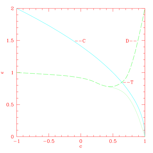
  Figure 1: Percolation phase diagram of the $O(3)$ model on the $\mathbb{T}$ lattice. C is the line $c=1-\epsilon^{2}/2$; above the dashed line D $\cal S_{\epsilon}$ percolates, above the dotted line $\langle\cal S_{\epsilon}\rangle<\infty$.

  To corroborate our conclusion that for $c<0.76$ neither $\cal P\epsilon$ nor $\cal S_{\epsilon}$ percolates, we carried out a different analysis of the equatorial clusters with width $\epsilon=0.75$; this time we compared them to the clusters of $\cal P^{+}_{\epsilon^{\prime}}$, chosen such that the polar cap has the same area as the equatorial strip $\cal S_{\epsilon}$; also both sets cover the same fraction of the lattice. The ratio $r^{\prime}(L)=\langle\cal P^{+}_{\epsilon^{\prime}}\rangle/\langle\cal S_{\epsilon}\rangle$ is always larger than 1, presumably because the polar cap has less boundary than the equatorial strip of the same area (in agreement with a conjecture stated in [31]). For small $c$ (roughly up to $c=0.4$) $r^{\prime}(L)$ shows a rapid increase with $L$, indicating that $\cal P_{\epsilon^{\prime}}$ forms rings (of all sizes) whereas the clusters of $\cal S_{\epsilon}$ have finite mean size. At $c\approx 0.4$ the behavior of $r^{\prime}(L)$ changes: it is still growing with $L$, but now only powerlike. This can only indicate that both kinds of clusters now form rings of arbitrary size; it rules out for all practical purposes that $S_{\epsilon}$ percolates, which would require a decrease to 0 as $L\to\infty$.

  The numerical results of this study are shown in Fig.2, taken from [5].

  

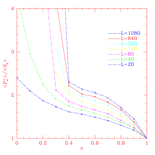
  Figure 2: The ratio of the mean cluster size of a polar cap of height 0.75 to that of an equatorial strip of the same height

  To sum up: our numerical study gives strong evidence that for sufficently small $\epsilon$ (about $<0.76$) $\cal S_{\epsilon}$ does not percolate for any value of $c$. This implies according to our results that for $c>1-0.76^{2}/2=0.745$ the correlation length $\xi=\infty$. The real challenge is of course to give a mathematical proof of this.

7 Where do we stand?

Clearly, the problem of AF is still open

• Textbook wisdom is insufficient to settle it positively

• Counterarguments are not rigorous

• Any progress towards proving or disproving AF is very desirable. For this reason programs such the one of K.R.Ito [32], attempting to prove AF by a controlled Renormalization Group approach, are very welcome.

A final remark: Solving the problem of AF for the $2D$ toy models which were mostly discussed here would be a big step towards understanding it also in $4D$ Yang-Mills theory and thereby also towards a solution of one of the Million Dollar Problems posed by the Clay Mathematics Institute.

References

- [1] J. M. Kosterlitz and D. J. Thouless, J. Phys. C 6 (1973) 1181.
- [2] J. Fröhlich , T. Spencer, Commun. Math. Phys. 83 (1982) 411.
- [3] A. Patrascioiu and E. Seiler, Phys. Rev. D 64 (2001) 065006.
- [4] A. Patrascioiu and E. Seiler, Phys. Rev. E 57 (1998) 111.
- [5] A. Patrascioiu and E. Seiler, J. Statist. Phys. 106 (2002) 811.
- [6] E. Brézin and J. Zinn-Justin, Phys. Rev. B 14 (1976) 3110.
- [7] E. T. Copson, Asymptotic Expansions, Cambridge University Press, Cambridge 1967.
- [8] F. Olver, Introduction to asymptotics and special functions, Academic Press, New York 1978.
- [9] N. D. Mermin and H. Wagner, Phys.Rev.Lett. 17 (1966) 1133.
- [10] R. L. Dobrushin and S. B. Shlosman, Commun.Math.Phys. 42 (1975) 31.
- [11] C. Pfister, Commun.Math.Phys. 79 (1981) 181.
- [12] J. Bricmont, J. R. Fontaine, J. L. Lebowitz, T. Spencer, Commun.Math.Phys. 78 (1980) 281.
- [13] S. Elitzur, Nucl. Phys. B 212 (1983) 501.
- [14] F. David, Phys. Lett. B 96 (1980) 371.
- [15] E. Seiler and K. Yildirim, J.Statist.Phys. 112 (2003) 457.
- [16] A. Patrascioiu and E. Seiler, Phys. Rev. Lett. (74 (1995) 1920.
- [17] J. L. Richard, Phys. Lett. B 184 (1987) 75.
- [18] A. Patrascioiu, J.L. Richard and E. Seiler, Phys. Lett. B 241 (1990) 229.
- [19] A. Patrascioiu, J.L. Richard and E. Seiler, Phys. Lett. B 254 (1991) 173.
- [20] A. Patrascioiu and E. Seiler, Phys. Lett. B 417 (1998) 314.
- [21] A. Patrascioiu and E. Seiler, Phys. Lett. B 532 (2002) 135.
- [22] M. Lüscher, P.Weisz and U. Wolff, Nucl. Phys. B 359 (1991) 221.
- [23] A. Patrascioiu and E. Seiler, J. Statist. Phys. 69 (1992) 573.
- [24] A. Patrascioiu and E. Seiler, Phys. Rev. Lett. 68 (1992) 1395.
- [25] A. Patrascioiu and E. Seiler, Nucl. Phys. Proc. Suppl. 30 (1993) 184.
- [26] A. Patrascioiu and E. Seiler, Percolation Theory and the Phase Structure of Two-Dimensional Ferromagnets in: CRM Proceedings and Lecture Notes 7 (1994) 153.
- [27] P. W. Kasteleyn and C. M.Fortuin, J. Phys. Soc. Jpn. 26 (Suppl.) (1969) 11; C. M. Fortuin and P. W. Kasteleyn, Physica 57 (1972) 536.
- [28] U. Wolff, Phys. Rev. Lett. 62 (1989) 361.
- [29] L. Russo, Z. Wahrsch. verw. Gebiete 43 (1978) 39.
- [30] M. Aizenman , J. Statist. Phys. 77 (1994) 351.
- [31] A. Patrascioiu, arXiv hep-lat/0002012.
- [32] K. R. Ito, these proceedings.