Vacuum Energy of Quantum Fields in Classical Background Configurations

Abstract

The ground state energy of a quantum field in the background of classical field configurations is considered. The subject of the ground state energy in framework of the quantum field theory is explained.

The short review of calculation methods (generalized zeta function and heat kernel expansion ) and its mathematical foundations is given.

We use the zeta-functional regularization and express the ground state energy as an integral involving the Jost function of a two dimensional scattering problem. We perform the renormalization by subtracting the contributions from first several heat kernel coefficients. The ground state energy is presented as a convergent expression suited for numerical evaluation. The investigation for three models has been carried out: scalar quantum field on the background of scalar string with rectangular shape, spinor vacuum polarized by magnetic string of the similar shape and spinor vacuum interacting with the Nielsen Olesen vortex. Using the uniform asymptotic expansion of the special functions entering the Jost function we are also able to calculate higher order heat kernel coefficients.

Several features of vacuum energy have been investigated numerically. We discuss corresponding numerical results.

Der Fakultät für Physik und Geowissenschaften

                              der Universität Leipzig

                                            eingereichte

                              D I S S E R T A T I O N

                   zur Erlangung des akademischen Grades

                              Doctor rerum naturalium

                                           (Dr.rer.nat)

                                             vorgelegt

von                Diplom Physiker (UA)               Igor Drozdov

geboren am 06.02.1970    in  Dnepropetrowsk, Ukraine


Leipzig, den 3.11/2003

1 Introduction

1.1 General remarks

The vacuum energy is a spectacular manifestation of the quantum nature of the real objects, in particular the fields of matter. In the framework of natural science it is also a powerful tool for investigation and of fundamental properties of our world.

It is a really non-trivial fact, that quantum field can be observable even in the case that there are no real particles of it present. The reason for this phenomena is one of the main properties inherent basically to any quantum system, namely the existence of the ground state. Indeed, it is well known from such a simple example of a quantum mechanical system as the linear harmonic oscillator with the eigenfrequency $\omega$, that the energy spectrum of this system possesses the lowest state and the energy of this state $E^{0}$ is not zero but is proportional to the Planck constant

$$E^{0}=\frac{1}{2}\hbar\omega.$$ (1.1)

This fact is generally also an intrinsic feature of any quantum object. Here we mean first of all quantum fields, namely matter fields (fermionic fields) and fields of interaction (bosonic fields). It means, one can establish the existence of a quantum field in the nature without to observe any real particles (quantums) of this field, but only through non zero vacuum values of observables, that are measurable, for example the vacuum energy.

The main point of this phenomena is that the energy of the ground state of a quantum system is not defined absolutely, that applies by the way in general to the energy itself as a physical feature. It is defined generally with a relation to some other state. That is why the discussion about the vacuum energy of quantum field makes sense in correspondence to some external condition, under which it becomes visible (or measurable in physical sense). Such an external condition can be some boundary or some classical field interacting to the quantum one (background)

The most famous manifestation of the vacuum energy was the Casimir effect (H.B.G.Casimir 1948), which consist in an interaction between two parallel conducting plates playing the role of boundaries for the electromagnetic field in vacuum state. This effect was predicted theoretically in [26] and measured experimentally 10 years later.

Sometimes, all the problems concerning the calculation of vacuum energy under external conditions are being called ”Casimir energy”, including also the problems of vacuum polarization by classical backgrounds. Actually, the vacuum energy of quantum spinor field polarized by a special homogeneous magnetic background was calculated by W.Heisenberg and H.Euler in 1936, 11 years before the discovery of the Casimir force.

1.2 Motivation

The investigation of vacuum effects in general and vacuum energy in particular has a number of applications to wide variety of physical problems (see recent reviews [23, 65, 62]). Indeed, in a lot of problems concerning the experiments in particle physics, certain effects caused by interaction with vacuum fluctuations must be taken into account as radiation corrections. For example in the bag model of hadrons in Quantum Chromodynamics the vacuum energy of quark and gluon fields makes essential contributions in the total nucleon energy. As further examples of such measurements one can refer to the experiments for the exact mass, isotopic charge, anomalous magnetic moment and so on.

Generally speaking, the vacuum corrections are more or less relevant in all problems of particle and high energy physics.

Moreover, one can imagine a situation that only the sole possibility to establish the existence of a quantum field in the nature, (since it is present in the model) is the interaction of its vacuum with an observable classical background (and measurable effects reasoned thereby). Actually, the interaction of the classical field configuration with quantum fields being in vacuum state leads to modification of macroscopic physical features of this classical object. In particular the energy and its dependence on the external parameter of this configuration undergoes an alteration. This interplay between the quantum vacuum and classical field is also called sometimes ”Casimir effect”. The modification of classical energy by vacuum corrections for real objects is usually negligible small. However, one can imagine some special field configurations such that the quantum corrections become comparable with the classical energy of the background.

Therefore it is a reasonable question to ask: could the quantum fluctuations change the main physical properties of classical object? First of all, the question concerns the stability (or instability) of field configurations.

For example, one can look for a field configuration, that acquires stability through an interaction with the quantum vacuum, although it would be instable in pure classical approach.

In particular, the issue of stability of strings is of interest. In electroweak theories, and in QED in particular, the coupling is small. Hence the vacuum energy (being a one loop correction to the classical energy) is suppressed by this coupling and indeed in most of the cases is not sufficient to change the stability properties. While in QED a magnetic string is intrinsically unstable, in electroweak theory there are unstable and stable configuration. Here quantum corrections may become important for the stability. A question of special interest is whether a strong or singular background may have a quantum vacuum energy comparable to the classical one. Such an example is considered in the present work for two kinds of field.

The vacuum correction could provide stability to classical instable objects, but vice versa it could also destabilize classical stable objects. The good illustration for this speculation can be provided by the model with the vortex of the Nielsen-Olesen type. This configuration is known to be stable for any integer vorticity $n$, if the parameter $\beta<1$. If the $\beta>1$, then only the vortex with $n=1$ remains stable, all configurations with the vorticity $n>1$ decay into n simple vortices with $n=1$. The question arises there: could the quantum vacuum fluctuation modify the parameter $\beta$ in such a way that transition from stable configuration to instable one takes place? The corresponding model will be also considered in the following sections.

The results and techniques gained here can be also applied to the problems of cosmology and to Condensed Matter Physics.

In Mathematical Physics the investigation of vacuum polarization has stimulated the development of powerful regularization and renormalization techniques based on the use of zeta function and heat kernel expansion, which are also considered below.

The subject of the work is restricted on the investigation of ground state energy of vacuum fields in presence of classical static field configurations with cylindrical and translational symmetry.

1.3 Historical review

Some people claim, that the subject of vacuum energy has no sense since this value is originally infinite. This point of view is in principal true, but the fact of Casimir force between two plates suggests the simple thought: if two plates are positioned with the distance $d$ from each other, the photon vacuum possesses really an infinite energy, and for the distance $d^{\prime}$ the vacuum energy is infinite as well, but not the same, and crucial for the problem is that the difference between these two values is finite and moreover measurable.

The same concerns the vacuum energy of quantum field, polarized by some external background. The first known example was the calculation of the vacuum energy of a spinor field in the background of a magnetic field. This problem was first considered as early as in 1936 by W. Heisenberg and H. Euler [53]. They were interested in the effective action in the background of a homogeneous magnetic field. It turned out that the global energy of spinor vacuum in presence of constant homogeneous magnetic field (the whole space is filled uniform by the field of magnitude $\vec{B}$) depends on this magnitude non trivialy. In particular the characteristic behaviour for the vacuum energy in the asymptotics of strong potential $B\rightarrow\infty$ in the form

$$E^{0}\sim B^{2}\ln B$$ (1.2)

was obtained.

Since the classical work [26] of H.B.G. Casimir, where the energy $E^{0}$ of vacuum polarized by two conducting planes was calculated analytically with the finite result

$$E^{0}=\frac{\pi^{2}}{720}\frac{\hbar c}{a^{3}}S,$$ (1.3)

a number of similar problems was investigated for various external conditions (boundary conditions, background potentials etc.). One may consult, for example, in the recent review [23] or the books [65, 62].

The discovery of the Aharonov-Bohm effect [3] gave rise to a series of works researching various approaches to the vacuum in presence of configurations similar to the Aharonov-Bohm string, so the vacuum in gauge theories claims its non trivial geometrical and topological structure, that is closely connected with the structure of gauge groups.

In this way local properties of photon and electron vacuum have been actively investigated. There it has been shown that the structure of vacuum state possesses a more reach variety of features as merely the global ground state energy [48]. In particular the subjects of interest were various local effects such as distribution of the vacuum energy density [75], vacuum currents [38], [58] and the backreaction (so called “feedback effects”) [58].

The other important application of the external field problem is the problem of non stationary vacuum under external conditions. This activity includes all the effects of particle creation by time dependent boundaries [81], or non conservative backgrounds, e.g., electric field. The most concerned problems were investigated in early 70’s, like [66], the results were restricted and confirmed for reduced space dimension [32] and generalized for arbitrary high dimension [41]. This interest was also motivated to explain of Hawking radiation of black holes.

The class of investigated backgrounds is usually restricted by the complication and solvability of a certain problem. In applications of bag models [37], [27] or in cosmology the spherical symmetric backgrounds are considered [17, 35, 21], for string like models the cylindrical symmetry is present [67, 2, 20].

Pure analytical calculations are only possible for simplest configurations, e.g. for the considered classical sample of homogeneous field [53],[59] or a very specific ones such as the transparent reflectionless domain wall [34]. For more complicated cases a number of alternative numerical approaches has been developed [68, 57, 44]. In the present work we restrict ourselves on the problems which can be treated analytically, (or analytically to some degree, demanding finally numerical evaluations [19, 20, 71, 33, 7])

Although a variety of problems for various backgrounds and in many QFT models have been successfully investigated, and a corresponding experience in handling these problems have been gained, the general understanding of the problem is so far not complete, and many features are still unclear.

The main open question is that no general rule for the dependence of the vacuum energy on the background properties has been found so far. In particular, it is unknown how to forecast the sign of the energy. Some special cases only has been recently investigated. An interesting approach is that used e.g. in [40] where the issue of the sign and of bounds on fermionic determinants in a magnetic background had been considered.

1.4 Examlpes

In QED, for the background of a flux tube with constant magnetic field inside the ground state energy was calculated in [20]. It turned out to be negative remaining of course much smaller than the classical energy of the background field.

The remarkably simple case of a magnetic background field concentrated on a cylindrical shell (i.e., a delta function shaped profile) was considered in [72]. Here different signs of the vacuum energy turned out to be possible in dependence on the parameters (radius and flux). However one has difficulties with a physical interpretation of this result since the model possesses an infinite classical energy density. So one needs a consequent interpretation in a suitable limit, as for example was done for an infinite thin Aharonov-Bohm string [42, 7]. Here a somewhat intermediate model between the rectangular potential [20] and $\delta$-shaped potential [72] is investigated in the present work.

An interesting approach is that used in [40] where the issue of the sign and of bounds on fermionic determinants in a magnetic background had been considered.

Presently, the interest is shifted to string like configurations. In [51] the contribution of the fermionic ground state energy to the stability of electroweak strings was addressed. In [30] the gluonic ground state energy in the background of a centrum-of-group vortex in QCD has been considered.

The ground state energy for vortex type solutions in gauge models with minimal coupling has been calculated implementing special numerical and partially analytical approaches to U(1) [57] and more complicated SU(2) and SU(3) theories [13]. In the case of supersymmetry the sufficient simplification is established through the high symmetry, that allowed to calculate recently a non-zero vacuum correction to the mass [79] and to the central charge [69] of the SUSY N=2 vortex. In the present work the result of [13] are extended to the vortex of Nielsen-Olesen type in the simplest U(1) abelian Higgs model.

1.5 The aim of the work

The main goals of the present research are:

Methodologically, an improvement of the existent technical tools to calculate the ground state energy in classical backgrounds is of interest as well as the applicability of these technics for more complicated configurations.

Physically, the influence of the quantum corrections on the background, in particular on the stability properties of the field system at all, and the asymptotic behaviour of the one-loop vacuum contribution to the total energy, are to be investigated by using the applied method.

1.6 The method

The class of considered problems to which we are restricted in the present work excludes basically all the problems with non stationary vacuum, since the method used below is not developed for such kind of models.

All the considered models contain one quantum field in vacuum state polarized by a classical background with special symmetry properties that simplify sufficiently the calculation procedure.

The expression for the ground state energy contains the ultraviolet divergences. To make the results of this calculations physically meaningful one has to extract the finite value from this infinite result, in other words it is necessary to subtract the ultraviolet divergences using some renormalization prescription.

There are various methods developed to get rid of non-physical divergences. In the present paper the zeta function regularization procedure has been used. This approach is well known and we follow in general [20]. Roughly speaking one has to subtract the contribution of the first few heat kernel coefficients ($a_{0}$ through $a_{2}$ in the given case of (3+1) dimensions). After that one can remove the intermediate regularization and one is left with finite expressions. However, in order to obtain these finite expressions in a form suitable for numerical calculations one has to go one step further. As described in [20, 19], see also below in Sec.5.4, one has to add and to subtract the certain part of the asymptotic expansion of the integrand.

In the present work we generalize the analysis done in [20, 71] of rectangular shaped background fields (scalar and magnetic) and, furthermore, for mixed background given in the from of numerical distribution.

The proceeding has been arranged consequently through the sections 3 - 6 simultaneously for the following three considered models.

We consider the vacuum energy of a spinor field in QED for a rectangular background, the scalar background with the same shape interacting to the scalar fluctuations, and finally the spinor vacuum polarized by the background configuration in form of the Nielsen-Olesen vortex in the abelian Higgs model.

The problem of the rectangular magnetic background reproduces in principle the main features of the one considered in [20], it is however technically more involved and allows progress in two directions. First, it allows to refine the mathematical and numerical tools for such problems and, second, it allows to address the question how the vacuum energy behaves for an increasingly singular background (making the rectangle narrower). So this model interpolates to some extend between the flux tube with homogeneous field inside in [20] and the delta shaped one in [72, 71].

The basic principles of this analytical calculation procedure are described in sections 3-5. We start with the well known zeta functional regularization. The regularized ground state energy is represented as a zeta function of a hamiltonian spectrum and treated in terms of the heat kernel expansion. A representation of the regularized ground state energy as an integral of the logarithmic derivative of the Jost function for wave scattering problem on the external background is obtained. The divergent part is identified as that part of the corresponding heat kernel expansion which does not vanish for large $m$ (mass of the quantum field). After the subtraction of this divergent part the remaining analytical expression must be transformed in order to lift the regularization . A part of the uniform asymptotic expansion of the Jost function is used for this procedure. The Jost function is obtained from the exact solutions of the equations of motion (these are the Klein-Gordon and Dirac equations respectively), derived in Sec.3.

The explicit form of exact and asymptotic Jost functions is considered in Sec.5.2 and 5.3. In Sec.5.1, 5.4 the representation useful for further numerical evaluations is derived. Sec.5.6 is devoted to the calculation of the heat kernel coefficient $a_{5/2}$ for the special magnetic background.

Finally the analytical expressions for the ground state energy are evaluated numerically. Sec.6 contains some numerical evaluations of the finite ground state energy for the considered models.

The ground state energy for the Nielsen-Olesen vortex background cannot be performed analytically since the background itself is given as the numerical solution of Nielsen-Olesen equations . In this case some analytical manipulations applied for the rectangular background have been replaced by the corresponding numerical procedures.

Additionally, the paper contains an introduction to the subject of ground state energy of quantum field in Sec.2.2. Some technical details are contained in the Appendix.

2 The ground state energy of quantized field

2.1 The effective action

In the generalized approach the contribution of the one-loop ground state energy appears as a first correction to the classical action in the so called ”effective” action. In order to derive this representation we start with the basic object of the quantum field theory in the functional integration approach namely the generating functional.

Let the action $S$ of the considered system consist of the classical field $\Phi$ and let the quantum field $\phi$ be defined in the canonical way as

$$S[\Phi,\phi]=S_{class}[\Phi]+\frac{1}{2}\int dx<\phi(x)K[\Phi]\phi(x)>,$$ (2.1)

where $\Phi$ is a classical field configuration called up from here and below ”background”, and $\phi$ is a quantized field, so called ”fluctuation”. The symbol $K[\Phi]$ relates to the kernel of the corresponding equation of motion, (the so called kernel of free action). It means particulary $K[\Phi]=\Box+m^{2}+V[\Phi]$ for scalar field with scalar potential $V$ and $K[A_{\mu}]=i\gamma^{\mu}(\partial_{\mu}-ieA_{\mu})-m$ for spinor field with the gauge background $A_{\mu}$. The edge brackets denote the full scalar product on the space of $\phi$. Proceeding from the defined action $S[\Phi,\phi]$ (2.1), we construct the related generating functional for Green functions of $\phi$

$$Z[\Phi,J]=\int{\cal D}\phi\exp\{iS[\Phi,\phi]+i\int\phi(x)J(x)dx\},$$ (2.2)

where the explicit dependence on the fluctuation $\phi$ does not appear, since it is integrated out. Here we have to notice, that we work in this paper with abelian background fields only. For non-abelian models the formula (2.2) is in general no more valid [43].

If we restrict the problem only to connected Green functions, the corresponding generating functional $W[\Phi,J]$ is related to the $Z[\Phi,J]$ by

$$Z[\Phi,J]=\exp\{iW[\Phi,J]\}.$$ (2.3)

One can formally restore the function $\phi(x)$ from the $W[\Phi,J]$ by the functional derivation

$$\phi(x)=\frac{\delta W[\Phi,J]}{i\delta J(x)}$$ (2.4)

and express the source parameter $J(x)$ with respect to the field variables

$$J=J[\Phi(x),\phi(x)].$$ (2.5)

This change of variables corresponds to the Legendre transformation $\{\Phi(x),J(x)\}\rightarrow\{\Phi(x),\phi(x)\}$. The effective action $\Gamma[\Phi(x),\phi(x)]$ is defined in terms of these new variables as

$$\Gamma[\Phi,\phi]=W[\Phi,J[\Phi,\phi]]-\int dx<\phi(x)J[\Phi(x),\phi(x)]>.$$ (2.6)

Using the Gaussian integral for the functional integrals of kind

$$\int\frac{d^{n}x}{\sqrt{2\pi}^{n}}e^{-Q(x)}$$ (2.7)

for any quadratic form $Q(x)=\frac{1}{2}<x,Kx>+<b,x>+\ c$ so that

$$\int\frac{d^{n}x}{\sqrt{2\pi}^{n}}e^{-(\frac{1}{2}<x,Kx>+<b,x>+c)}=\exp\{\frac{1}{2}<b,K^{-1}b>-c\}(\det K)^{-\frac{1}{2}}$$ (2.8)

for the functional integrals (2.2), one can calculate the generating functional $Z[\Phi(x),J(x)]$ explicit:

$$Z[\Phi,J]=e^{iS_{class}[\Phi]}(\det K[\Phi])^{\mp\frac{1}{2}}e^{-\frac{i}{2}<JK^{-1}J>}.$$ (2.9)

Here the $\det K[\Phi]$ is the functional determinant of the kernel of the free action $K[\Phi]$ (e.g. $\Box-m^{2}$, more examples for certain models are listed below, (Sec.3).

The choice of the sign of the power $(\det K[\Phi])^{\mp\frac{1}{2}}$ corresponds to the bosonic/ fermionic fields $\phi$ respectively. Using the known representation of the logarithm of determinant through the trace of logarithms

$$\ln\det K={\bf Tr\ }\ln K,$$ (2.10)

one can arrive for the connected generating functional $W[\Phi(x),J(x)]$ at

$$W[\Phi(x),J(x)]=S_{class}[\Phi]\pm\frac{i}{2}{\bf Tr\ }\ln K-\frac{1}{2}<JK^{-1}J>$$ (2.11)

and for the effective action (2.6)

$$\Gamma[\Phi(x),\phi(x)]=S_{class}[\Phi]\pm\frac{i}{2}{\bf Tr\ }\ln K+\frac{1}{2}<\phi K^{-1}\phi>.$$ (2.12)

If the quantum field $\phi$ is considered only in the ground state, the corresponding effective action reads

$$\Gamma[\Phi(x),\phi(x)]|_{\phi=0}=\Gamma[\Phi(x)],$$ (2.13)

whereat it is supposed that there is no spontaneously broken symmetry of the ground state.

The zeta-functional regularization formalism can be applied to the effective action in the form (2.13). The corresponding zeta function - regularized effective action is considered in the (Sec. 4)

2.2 The ground state energy in the framework
of canonical quantization

The explicit expression for calculation of the ground state energy can be derived also from the canonical quantization formalism, that we even use. In the following work two kinds of quantum field are discussed-the Klein-Gordon scalar field and the Dirac spinor field.

2.2.1 Quantized scalar field

Consider a simplest case of the real massive scalar field $\varphi$ with the lagrangian

$${\cal L}=\frac{1}{2}\{\partial_{\mu}\varphi\partial^{\mu}\varphi-m^{2}\varphi^{2}\}$$ (2.14)

leading to the Klein-Gordon equation

$$\left\{\Box+m^{2}\right\}\varphi(\vec{x},t)=0$$ (2.15)

All the further discussions and calculations are concerned with the Minkowski space-time $g_{\mu\nu}=diag\{1,-1,-1,-1\}$. Then the (2.15) will be rewritten as

$$\left\{\frac{\partial^{2}}{\partial{x^{0}}^{2}}-\Delta+m^{2}\right\}\varphi(\vec{x},t)=0.$$ (2.16)

Since the equation is of second order with respect to time $t=x^{0}$, we can define so called ”positive-” and ”negative-frequency” solutions $\varphi^{+}(\vec{x},x^{0})$ and $\varphi^{-}(\vec{x},x^{0})$.

The further explanation follows the textbook [11]. Let the equation of motion have a continuous spectrum of solutions $\varphi^{\pm}(\vec{x},x^{0})$. The $\varphi(x)$ are representable as the Fourier integral:

$$\varphi(x)=\frac{1}{(2\pi)^{3/2}}\int\limits_{-\infty}^{\infty}\frac{d^{3}k}{\sqrt{2k_{0}}}\left[e^{(-ik_{0}x^{0})}e^{(i\vec{k}\vec{x})}\varphi^{-}(k_{0},\vec{k})+e^{(ik_{0}x^{0})}e^{-i(\vec{k}\vec{x})}\varphi^{+}(k_{0},\vec{k})\right].$$ (2.17)

The normalization of the solutions is kept to be the one used in [11], but for our problems it is unimportant. The sign switch of the frequency $\theta(k_{0})$ is supposed to be contained in the corresponding Fourier images $\varphi^{\pm}(k_{0},\vec{k})$.

We consider the problems with the translational invariance along the z-axis. It means, the z-variable is not present in the equation of motion explicitly. The solution of the equation (2.16) may contain only the s z-dependent factor of kind $e^{\pm(ip_{z}z)}$ and this factor can be separated for the next step.

The energy of quantum field will be understood by means of the 00-component of the canonical energy momentum tensor $T^{\mu\nu}$, that is defined for a given lagrangian ${\cal L}$ as

$$T^{\mu\nu}=\frac{\partial{\cal L}}{\partial(\partial_{\mu}\varphi)}\partial^{\nu}\varphi-g^{\mu\nu}{\cal L}$$ (2.18)

For the zero-zero component of $T^{\mu\nu}$ (the hamiltonian density) of the neutral scalar field we have

$${\cal H}(x)=T^{00}(x)=\frac{1}{2}\left\{[\partial_{0}\varphi(x)]^{2}+[\nabla\varphi(x)]^{2}+m^{2}\varphi(x)^{2}\right\}$$ (2.19)

By (2.19) we have derived the explicit from of the hamiltonian density (energy density per unit volume) of the field $\varphi$. Then the resulted function of coordinates $T^{00}(x)$ describes a local spatial distribution of the energy of scalar field $\varphi$

The energy contained in the finite volume V can be obtained through the integration over $d^{3}x$. Suppose we are interesting for the energy of the field contained in the layer of finite thickness $L$ between two plates transversal to the axis $z$, say $z=0$ and $z=L$. The global field energy contained in this layer is the integral

$$E_{L} = \int T^{00}=\frac{1}{2}\int\limits_{0}^{L}dz\int d^{2}x\int\frac{d^{3}p\ d^{3}k}{2\sqrt{k_{0}p_{0}}}$$

$$\left\{-k_{0}p_{0}[\varphi^{+}(p)\varphi^{+}(k)e^{ix_{0}(k_{0}+p_{0})}e^{-i(\vec{k}+\vec{p})\vec{x}}+\varphi^{-}(p)\varphi^{-}(k)e^{-ix_{0}(k_{0}+p_{0})}e^{i(\vec{k}+\vec{p})\vec{x}}-\right.$$

$$\left.\varphi^{+}(p)\varphi^{-}(k)e^{-ix_{0}(k_{0}-p_{0})}e^{i(\vec{k}-\vec{p})\vec{x}}-\varphi^{-}(p)\varphi^{+}(k)e^{ix_{0}(k_{0}-p_{0})}e^{-i(\vec{k}-\vec{p})\vec{x}}]\right\}$$

The first and the second summand turn out to be equal zero if the integration over $d^{3}x$ is performed, in the remaining two terms the part, containing the dependence on z-variable can be separated and the integration over $dz$ builds the Fourier representation of delta-function $\delta(p_{z}-k_{z})$, that reads

$$\delta(x)=\int\limits_{-\infty}^{\infty}\frac{dp}{2\pi}e^{-ipx}$$ (2.20)

Finally one arrives at the form:

$$E_{L}=\int T^{00}=\frac{1}{2}L\int\frac{dp_{z}}{2\pi}\int d^{2}p\ p_{0}[\varphi^{+}(p)\varphi^{-}(p)+\varphi^{-}(p)\varphi^{+}(p)]$$ (2.21)

where the remaining components of the momentum space are denoted as $d^{2}p$. Divided by $L$ this value means the energy density per unit length.

The canonical secondary quantization procedure (for bosonic scalar field) means the decomposition of the arbitrary solution $\varphi(x,t)$ of (2.15) onto the eigenfunctions $\varphi^{\pm}_{n}$

$$\varphi(x,t)=\int\frac{d^{3}k}{(2\pi)^{3}2\omega_{k}}[a(k)e^{-ikx}+a^{+}(k)e^{ikx}]$$ (2.22)

with the coefficients $a(k),a^{+}(k)$ called the annihilation and creation operators with the momentum $k$. The integration is carried out with the invariant measure on-shell,[11, 70], $\omega_{k}=\sqrt{\vec{k}^{2}+m^{2}}$.

The commutation relations between $a(k),a^{+}(k)$ implied by the normalization conditions in the Fock space [11] are

$$[a(k),a^{+}(k^{\prime})]=\delta(k-k^{\prime});\ \ \ [a^{+}(k),a^{+}(k^{\prime})]=[a(k),a(k^{\prime})]=0$$ (2.23)

Within these relation the hamiltonian ${\cal H}$ takes the form

$$H=\int\frac{d^{3}k}{(2\pi)^{3}2k_{0}}\frac{k_{0}}{2}\left[a^{+}(k)a(k)+a(k)a^{+}(k)\right]=\int\frac{d^{3}k}{(2\pi)^{3}2k_{0}}k_{0}\left[N(k)+\frac{1}{2}\right],$$ (2.24)

where $N(k)=a^{+}(k)a^{(}k)$ is the operator of number of particles with the momentum $k$.

The vacuum state is understood as the lowest state of the quantum field in the Fock space is the vacuum state $|0>$ defined by

$$a(k)|0>=0,$$ (2.25)

and the corresponding co-state $<0|$ respectively

$$<0|a^{+}(k)=0$$ (2.26)

Now we define the vacuum energy as a vacuum expectation value of $T^{00}$ in the vacuum state

$$E_{vac}=\int<0|\ T^{00}\ |0>.$$ (2.27)

All problems considered below in this paper concerns with the backgrounds possessing translational symmtery along the $z$-axis, it is integrated over the $z$-component of the momentum, $p_{z}/(2\pi)$ and the transversal component of the momentum, $\vec{p}$ (say, for cylindrical coordinates $\vec{p}\equiv\vec{p}_{r\varphi}$), can be quantized, so that it acquires discrete values $\vec{p}_{(}n)$. Then, by means of the integration measure of Fourier transformations [80], the integration over $\frac{dp}{2\pi}$ will be substituted by summation over $p_{(}n)$ . Since we mention the vacuum state as a state without real particles, it leads to the relation

$$E_{vac}=\frac{1}{2}\int\frac{dp_{z}}{2\pi}\int\frac{d^{2}p}{(2\pi)^{2}}\omega_{p}=\int\frac{dp_{z}}{2\pi}\sum\limits_{(n)}\omega_{(n)}$$ (2.28)

The (2.25,2.26), substituted into the (2.21), provide the final expression for vacuum energy density ${\cal E}$ per unit length of the translational invariant field configuration

$${\cal E}=\int T^{00}=\frac{1}{2}\int\frac{dp_{z}}{2\pi}\sum\limits_{(n)}\omega_{(n)}$$ (2.29)

where $\omega_{n}=\sqrt{\vec{p_{n}}^{2}+m^{2}}$ are the eigenvalues of the hamiltonian (2.19).

Here it is suitable to notice that the solutions $\varphi(x)$ of the Klein-Gordon equation should be orthonormalized with respect to the inner product for scalar field, but the normalization coefficients of the eigenfunctions $\varphi_{(n)}(x)$ does not appear in the final expression of the ground state energy because we handle here with the eigenvalues only; thus the discussion concerning the normalization coefficients can be omitted for our problem.

Thus we obtained that the vacuum energy defined by 2.27 is equal to the half of sum over the spectrum of eigenvalues of hamiltonian, that has been first defined as the ground state energy energy. Therefore the both definitions coincide with. However, it is necessary to notice that this equivalence is true for a system of not interacting (“free”) fields. It will be mentioned further in Sec.4 in context of the effective action.

2.2.2 Quantized Dirac field

Let the quantum field $\psi(x)$ now be the 4-component spinor field with the free lagrangian

$${\cal L}=\frac{i}{2}\left\{\bar{\psi}(x)\gamma^{\mu}\partial_{\mu}\psi(x)-\partial_{\mu}\bar{\psi}(x)\gamma^{\mu}\psi(x))\right\}-m\bar{\psi}(x)\psi(x),$$ (2.30)

and the spinor function $\psi(x)$ obeys the Dirac equation

$$(i\gamma^{\mu}\partial_{\mu}-m)\psi(x)=0$$ (2.31)

One can use however the simplified lagrangian that also leads to the equation (2.31), namely

$${\cal L}=\bar{\psi}(x)\left\{i\gamma^{\mu}\partial_{\mu}-m\right\}\psi(x)$$ (2.32)

The canonical energy-momentum tensor corresponding to the (2.30) reads

$$T^{\mu\nu}=\frac{i}{2}\left\{\bar{\psi}(x)\gamma^{\mu}\partial^{\nu}\psi(x)-\partial^{\nu}\bar{\psi}(x)\gamma^{\mu}\psi(x)\right\}-g^{\mu\nu}{\cal L}$$ (2.33)

For simplicity we work here with the short form (2.32). The corresponding energy-momentum tensor $T^{\mu\nu}$ is

$$T^{\mu\nu}(x)=\bar{\psi}(x)\gamma^{\mu}\partial_{\mu}\psi(x)$$ (2.34)

and the 00-component of them, that we are interested in, is the corresponding hamiltonian density ${\cal H}(x)$, that is defined as

$${\cal H}(x)=T^{00}(x)=\bar{\psi}(x)\gamma^{0}\partial_{0}\psi(x)$$ (2.35)

Let the solutions of the Dirac equation be $\psi^{+}$ and $\psi^{-}$, which are normalized by

$$\int d^{3}x\psi^{\dagger}(x)\psi(x)=1,$$ (2.36)

what will be no further discussed since the normalization of wave functions does not play any role in the resulting ground state energy (the remark in the end of the previous subsection).

Now use again the decomposition on the states with positive and negative frequences for each of solutions $\bar{\psi}(x),\psi(x)$ as in the scalar case above,

$$\psi^{\pm}(x)=\frac{1}{(2\pi)^{3/2}}\int d^{3}ke^{\pm ikx}\sum\limits_{\nu=1,2}a^{\pm}_{\nu}(\vec{k})v^{\nu\pm}(\vec{k})$$ (2.37)

$$\bar{\psi}^{\pm}(x)=\frac{1}{(2\pi)^{3/2}}\int d^{3}ke^{\pm ikx}\sum\limits_{\nu=1,2}\bar{a}^{\pm}_{\nu}(\vec{k})\bar{v}^{\nu\pm}(\vec{k})$$ (2.38)

the index $\nu$ enumerates the two states with different spin projections, $v^{\nu\pm}(\vec{k})$ and $\bar{v}^{\nu\pm}(\vec{k})$ are the 4-component spinor amplitudes, spinor indices are omitted.

The resulting hamiltonian density expressed through the amplitudes reads

$$T^{00}=\int d^{3}k\ k_{0}e^{\pm ikx}\sum\limits_{\nu=1,2}[\bar{a}^{+}_{\nu}(\vec{k})a^{-}_{\nu}(\vec{k})-\bar{a}^{-}_{\nu}(\vec{k})a^{+}_{\nu}(\vec{k})]$$ (2.39)

The secondary quantized spinor field in the canonical formalism will be represented as

$$\psi(x)=\psi^{+}(x)+\psi^{-}(x),\ \ \ \ \bar{\psi}(x)=\bar{\psi}^{+}(x)+\bar{\psi}^{-}(x)$$ (2.40)

where the creation and annihilation operators $\bar{a}^{+}_{\nu},{a}^{-}_{\nu}$ and $\bar{a}^{-}_{\nu},{a}^{+}_{\nu}$ obey now the anticommutation relations in order to have a positive definite form for the energy.

$$\{\bar{a}^{+}_{\mu}(\vec{k}),{a}^{-}_{\nu}(\vec{k}^{\prime})\}=\delta_{\mu\nu}\delta(\vec{k}-\vec{k}^{\prime})$$ (2.41)

$$\{\bar{a}^{-}_{\nu}(\vec{k}),{a}^{+}_{\nu}(\vec{k}^{\prime})\}=\delta_{\mu\nu}\delta(\vec{k}-\vec{k}^{\prime})$$ (2.42)

$$\{\bar{a}^{+}_{\mu}(\vec{k}),{a}^{+}_{\nu}(\vec{k}^{\prime})\}=\{\bar{a}^{-}_{\mu}(\vec{k}),{a}^{-}_{\nu}(\vec{k}^{\prime})\}=$$ (2.43)

$$\{\bar{a}^{+}_{\mu}(\vec{k}),\bar{a}^{-}_{\nu}(\vec{k}^{\prime})\}=\{{a}^{+}_{\mu}(\vec{k}),{a}^{-}_{\nu}(\vec{k}^{\prime})\}=0$$ (2.44)

By applying the creation/annihilation operators ${a}^{\pm}$ and complex (but not Hermitian) conjugated $\bar{a}^{\pm}$ of them to the vacuum state

$$<0|\bar{a}^{+}={a}^{-}|0>=0$$ (2.45)

$$<0|{a}^{+}=\bar{a}^{-}|0>=0,$$ (2.46)

one arrives at the vacuum expectation value for this hamiltonian

$$H=-2\sum\limits_{(n)}\omega_{(n)}.$$ (2.47)

For translational invariant problem the corresponding energy density per unit length is

$${\cal E}=-4\int\frac{dp_{z}}{2\pi}\ \frac{1}{2}\sum\limits_{(n)}\omega_{(n)}$$ (2.48)

Thus the hamilonian density, that involves the summation over 2 states with different sign of energy ( fermoin and anti-fermion energies ) distinguished by the sign of mass, and over 2 spin projection states, compared with this one for the scalar field (2.29 of the previous subsection) acquires the resulting multiplicative factor -4.

In the following sections the formulae (2.48 and 2.29) will be used as a starting point for calculations of the ground state energy .

3 The equations of motion and solutions

We consider basically the field system which consists of quantum fields $\phi$ (fluctuations) interacting with classical fields $\Phi_{i}$ of fixed geometrical configurations (backgrounds).

The corresponding lagrangian is constructed as

$${\cal L}={\cal L}_{\Phi_{i}}+{\cal L}_{\phi}+{\cal L}_{int},$$ (3.1)

where ${\cal L}_{int}$ is an interaction between $\phi$ and $\Phi_{i}$. The background $\Phi_{i}$ must not necessary satisfy any field equations. This simplified approach is somewhat physically incomplete but it allows to reduce the problem to solutions for quantum fluctuations only, that are supposed to obey the corresponding equations of motion with the background field as parameter. Generally speaking, the introduction of an external background field in a quantum field model is not trivial and not unique (see for example [76]).

A more consistent approach treats any field as consisting of a background part and fluctuations [50], [29].

The total energy density of the system is the sum of the classical and quantum parts

$${\cal E}={\cal E}^{cl}+{\cal E}^{\phi},$$ (3.2)

where ${\cal E}^{cl}$ is the local energy density as a function of coordinates of backgrounds ${\Phi_{i}}$ defined as the 00-component of the canonical energy-momentum tensor

$${\cal E}^{cl}(x)=\sum\limits_{i}{\cal E}^{\Phi_{i}}(x)=\sum\limits_{i}T^{00}_{\Phi_{i}}(x),$$ (3.3)

and the quantum part is the vacuum expectation value of the canonical hamiltonian of quantum field ${\phi}$. It is assumed that a considered problem is static and the vacuum state in the Fock space is defined in such a way that the constructed object is local:

$${\cal E}^{\phi}(x)={\cal E}^{\phi}_{0}=<0|{\cal H}(x)|0>.$$ (3.4)

The object defined in such a way is generally speaking non-local, because it depends on the background potential in the whole space. The integral of it over the space provides however a well defined global object, which we are even interested in, see below. The ${\cal E}^{\phi}$ has been shown in Sec.(2.2) to be proportional to the sum over the spectrum of ${\cal H}$

$${\cal E}^{\phi}_{0}=\frac{1}{2}\sum\limits_{(n)}\omega_{(n)}.$$ (3.5)

Here the spectrum is defined as usual

$${\cal H}\Phi_{n}(x)=\omega_{n}^{2}\Phi_{n}(x),$$ (3.6)

and is supposed here to be discrete for technical reasons.

The energy ${\cal E}$ is treated as the density per unit volume. Since we are interested in the global energy $E$ of the field system, it should be integrated over the volume V,

$$E=\int\limits_{V}d^{3}x\ {\cal E}(x).$$ (3.7)

3.1 The scalar field with the scalar background

Consider first a simple model described by the lagrangian density

$${\cal L}=\frac{1}{2}\{\partial_{\mu}\phi\partial^{\mu}\phi-m^{2}\phi^{2}+\partial_{\mu}\Phi\partial^{\mu}\Phi-M^{2}\Phi^{2}\}-V(x)\phi^{2}+[\lambda\Phi^{4}]$$

$$V(x)=\alpha\Phi(x)^{2},$$ (3.8)

where the field $\phi$ is a quantum fluctuation interacting with a scalar background field $\Phi(x)$. The lagrangian can also contain the self-interaction term $\lambda\Phi^{4}$. It will be shown later that such a term is needed for the interpretation of a counter term arising from the quantum vacuum fluctuations $\phi$ and leading to a renormalization of the self-interaction coupling constant $\lambda$.

The corresponding classical energy density of the background and the vacuum energy can be obtained in a standard way and they are

$${\cal E}^{cl}=\frac{1}{2}\{\partial_{0}\Phi\partial^{0}\Phi+(\nabla\Phi)^{2}+M^{2}\Phi^{2}\}$$ (3.9)

$${\cal E}^{\phi}=\frac{1}{2}<0|\partial_{0}\partial^{0}+\nabla^{2}+m^{2}+V(x)|0>.$$ (3.10)

The equation of motion for the fluctuations $\phi$ corresponding to the (3.8) is the Klein-Gordon equation :

$$(\partial_{0}\partial^{0}-\Delta+m^{2}+V(x))\phi(x)=0$$ (3.11)

From now on we restrict ourselves to cylindrically symmetric potentials $V(x)=V(r)$

For the scalar field $\phi(x)$ in cylindrical coordinates $(\varphi,r,z)$ it is usual to make the ansatz

$$\phi(x)=\phi(r)e^{-ip_{0}x^{0}}e^{-il\varphi}e^{-ip_{z}z},$$ (3.12)

which leads to an ordinary second order equation for the radial part:

$$\left\{\frac{\partial^{2}}{\partial r^{2}}+\frac{1}{r}\frac{\partial}{\partial r}+\left(k^{2}-V(r)-\frac{l^{2}}{r^{2}}\right)\right\}\phi(r)=0,$$ (3.13)

with $k^{2}\equiv p_{0}^{2}-m^{2}$. This is an ordinary equation of the Bessel type, known to have an analytical solution representable in terms of the Bessel functions.

The rectangular shaped scalar potential

Suppose the construction of the background potential looks as follows:

$$V(r)=\left\{\begin{array}[]{cc}V_{0}=const&R_{1}<r<R_{2}\\ 0&otherwise\end{array}\right.$$ (3.14)

Then (3.13) has the following solutions in the domains restricted by the cylinders $r=R_{1}$ and $r=R_{2}$:

$$I.\ \ \ r<R_{1}\ \ \phi_{k,l}^{I}(r)=C^{I}J_{l}(kr)$$

$$II.\ \ \ R_{1}<r<R_{2}\ \ \phi_{k,l}^{II}(r)=C^{II}_{1}H^{(1)}_{l}(qr)+C^{II}_{2}H^{(2)}_{l}(qr)$$

$$III.\ \ \ r>R_{2}\ \ \phi_{k,l}^{III}(r)=C^{III}_{1}H^{(1)}_{l}(qr)+C^{III}_{2}H^{(2)}_{l}(qr)$$ (3.15)

Here $q=\sqrt{k^{2}-V_{0}}$, $C_{i}$ are some normalization coefficients. If the solution $\phi_{k,l}^{I}(r)$ is chosen to be regular in $r\rightarrow 0$, then the coefficients $C^{III}_{2}$ and $C^{III}_{1}$ are the corresponding Jost function $f_{l}(k)$ and its complex conjugated, $\bar{f}_{l}(k)$, (which will be discussed later, see Sec.5.2).

3.2 The Dirac spinor field with the magnetic background

The next model to consider is the spinor electrodynamics:

$${\cal L}=-\frac{1}{4}F_{\mu\nu}F^{\mu\nu}+\bar{\psi}[i\gamma^{\mu}(\partial_{\mu}-ieA_{\mu})-m]\psi,$$ (3.16)

where the $A_{\mu}$ is the classical electromagnetic background,

$$F_{\mu\nu}=\partial_{\mu}A_{\nu}-\partial_{\nu}A_{\mu},$$ (3.17)

as usual. We consider only a static problem. The background cannot depend on time and must be pure magnetic, the electric field is excluded, ${\bf E}=0$.

Like the scalar case considered above we derive the corresponding classical energy of the background and the vacuum energy of the spinor quantum fluctuations.

$${\cal E}^{cl}=\frac{1}{4}F_{\mu\nu}F^{\mu\nu}+F^{0\nu}F_{\nu}^{0}=\frac{1}{2}{\bf B}^{2},$$ (3.18)

where the ${\bf B}$ is the magnetic field,

$${\cal E}^{\psi}=<0|\gamma^{0}\partial_{0}\{\vec{\gamma}(-i\vec{\nabla}-e\vec{A})+m\}|0>$$ (3.19)

Let us chose the potential $A_{\mu}$ to be of a rectangular shape (like the scalar one discussed above):

$$\vec{A}=\frac{\Phi}{2\pi}\frac{a(r)}{r}\vec{e_{\varphi}},$$ (3.20)

so that it contains only the $A_{\varphi}$ component and possesses a cylindrical symmetry again. The radial part profile function $a(r)$ is taken to be

$$a(r)=\left\{\begin{array}[]{c}0,\hfill r<R_{1},R_{2}\\ \frac{1}{\kappa}(\frac{r^{2}}{R_{1}^{2}}-1)\ R_{1}\leq r\leq R_{2}\\ 1,r>R_{1},R_{2}\end{array}\right.\\$$ (3.21)

Then the profile function for the magnetic field ${\bf B}(r)=\frac{\Phi}{2\pi}h(r)\vec{e}_{z}$ is

$$\ \ h(r)=\frac{1}{r}\frac{\partial}{\partial r}a(r)=\left\{\begin{array}[]{c}0,\hfill r<R_{1},R_{2}\\ \frac{2}{\kappa R^{2}_{1}}R_{1}\leq r\leq R_{2}\\ 0,r>R_{1},R_{2}\end{array}\right.$$ (3.22)

with $\kappa=\frac{R_{2}^{2}-R_{1}^{2}}{R_{1}^{2}}$. The shape of the background can be interpreted geometrically as an infinitely long flux tube empty inside.

We proceed now with the Dirac equation for spinor field $\psi(x)$ of mass $m$ and charge $e$

$$\left\{i\gamma^{\mu}\frac{\partial}{\partial x^{\mu}}-m-e\gamma^{\mu}A_{\mu}\right\}\psi=0$$ (3.23)

where $A_{\mu}$ is given by (3.20). The gamma matrices in our representation are chosen as in [25, 9]:

$$\gamma^{0}=\left\{\begin{array}[]{cc}\sigma_{3}&0\\ 0&-\sigma_{3}\end{array}\right\}\ \ \ \ \ \gamma^{1}=\left\{\begin{array}[]{cc}i\sigma_{2}&0\\ 0&-i\sigma_{2}\end{array}\right\}$$ (3.28)

$$\gamma^{2}=\left\{\begin{array}[]{cc}-i\sigma_{1}&0\\ 0&i\sigma_{1}\end{array}\right\}\ \ \ \ \ \gamma^{3}=\left\{\begin{array}[]{cc}0&\ I\\ -I&\ 0\end{array}\right\},$$ (3.33)

$\sigma_{j}$ are the $2\times 2$ Pauli matrices, $I$ is the $2\times 2$ unit matrix.

Now we follow the standard procedure and separate the variables. Using the ansatz

$$\phi(r,\varphi,z)=e^{-ip_{0}x^{0}}e^{-ip_{z}z}\Psi(r,\varphi)\\$$ (3.34)

we obtain the equation for the 4- component spinor $\Psi(r,\varphi)=\left[\begin{array}[]{c}\phi(r,\varphi)\\ \chi(r,\varphi)\end{array}\right]$

$$\left\{\begin{array}[]{cc}p_{0}+\hat{L}-m\sigma_{3}&p_{z}I\\ \\ p_{z}I&p_{0}+\hat{L}+m\sigma_{3}\end{array}\right\}\Psi(r,\varphi)=0,$$ (3.35)

where $\hat{L}=i\sum\limits_{i=1}^{2}\sigma_{i}(\partial_{i}+ieA_{i})$, $\phi,\chi$ are the two-component spinors.

Respecting the translational invariance of the system it is convenient to solve the equations only for $p_{z}=0$. Then the system (3.35) decays in two decoupled equations, for $\phi$ and $\chi$ respectively, which are distinguished only by sign of mass $m$.

We consider the first of these two equations. By meaning of the standard ansatz

$$\phi(r,\varphi)=\left[\begin{array}[]{c}i\psi^{u}(r)e^{-i(l+1)\varphi}\\ \\ \psi^{l}(r)e^{-il\varphi}\end{array}\right],$$ (3.36)

( $l$ is the orbital quantum number), it reads:

$$\left\{\begin{array}[]{cc}p_{0}-m&\frac{\partial}{\partial r}-\frac{l-\Omega a(r)}{r}\\ \\ -\frac{\partial}{\partial r}-\frac{l+1-\Omega a(r)}{r}&p_{0}+m\end{array}\right\}\Phi(r)=0$$ (3.37)

Here the radial part $\Phi(r)$ denotes

$$\Phi(r)=\left\{\begin{array}[]{c}\psi^{u}(r)\\ \\ \psi^{l}(r)\end{array}\right\}$$ (3.38)

and

$$\Omega=\frac{e\Phi}{2\pi}.$$ (3.39)

In order to use later the symmetry properties of the Jost function we redefine the parameter $l$ in (3.36) (orbital number) as $\nu$ according to

$$\nu=\left\{\begin{array}[]{c}l+\frac{1}{2}\ for\ \ l=0,1,2,...\\ \\ -l-\frac{1}{2}\ for\ \ l=-1,-2,...\end{array}\right.$$ (3.40)

For the given construction of potential (3.21) we get three equations and three types of solutions for 3 areas of space respectively:

Domain I: $r<R_{1}$. The free wave equation (the magnetic flux is zero), the solutions are the Bessel functions $J_{\nu\pm\frac{1}{2}}(kr)$

$$\Phi_{I}^{-}(r)=\left[\begin{array}[]{c}\psi^{u-}_{I}(r)\\ \\ \psi^{l-}_{I}(r)\end{array}\right]={\frac{1}{\sqrt{p_{0}-m}}\left[\begin{array}[]{c}-\sqrt{p_{0}+m}J_{\nu-\frac{1}{2}}(kr)\\ \\ \sqrt{p_{0}-m}J_{\nu+\frac{1}{2}}(kr)\end{array}\right]},$$ (3.43)

$$\Phi_{I}^{+}(r)=\left[\begin{array}[]{c}\psi^{u+}_{I}(r)\\ \\ \psi^{l+}_{I}(r)\end{array}\right]={\frac{1}{\sqrt{p_{0}-m}}\left[\begin{array}[]{c}\sqrt{p_{0}+m}J_{\nu+\frac{1}{2}}(kr)\\ \\ \sqrt{p_{0}-m}J_{\nu-\frac{1}{2}}(kr)\end{array}\right]}$$ (3.46)

$p_{0}=\sqrt{m^{2}+k^{2}}$
This solution of equation (3.37) in the domain I is chosen to be the so called regular solution which is defined as to coincide for $r\rightarrow 0$ with the free solution.

Domain II: $R_{1}<r<R_{2}$ The equation with a homogeneous magnetic field $\frac{\Omega}{e}h(r)=\frac{\Omega}{e}\frac{2}{\kappa R^{2}_{1}}$ has the solution

$$\Phi_{II}^{-}(r)=C_{r}^{-}\left[\begin{array}[]{c}\psi^{u-}_{II.r}(r)\\ \\ \psi^{l-}_{II.r}(r)\end{array}\right]+C_{i}^{-}\left[\begin{array}[]{c}\psi^{u-}_{II.i}(r)\\ \\ \psi^{l-}_{II.i}(r)\end{array}\right]=$$ (3.49)

$$C_{r}^{-}\left[\begin{array}[]{c}\frac{(p_{0}+m)}{2(\tilde{\alpha}+1)}r^{\tilde{\alpha}+1}e^{-\frac{\beta r^{2}}{4}}{{}_{1}}F_{1}(1-\frac{k^{2}}{2\beta},\tilde{\alpha}+2;\frac{\beta r^{2}}{2})\\ \\ \hfill r^{\tilde{\alpha}}e^{-\frac{\beta r^{2}}{4}}{{}_{1}}F_{1}(-\frac{k^{2}}{2\beta},\tilde{\alpha}+1;\frac{\beta r^{2}}{2})\end{array}\right]$$ (3.51)

(3.52)

$$+C_{i}^{-}\left[\begin{array}[]{c}\frac{1}{p_{0}-m}\frac{2\tilde{\alpha}}{r}(\frac{\beta r^{2}}{2})^{-\tilde{\alpha}}e^{-\frac{\beta r^{2}}{4}}{{}_{1}}F_{1}(-\frac{k^{2}}{2\beta}-\tilde{\alpha},-\tilde{\alpha};\frac{\beta r^{2}}{2})\\ \\ (\frac{\beta r^{2}}{2})^{-\tilde{\alpha}}e^{-\frac{\beta r^{2}}{4}}{{}_{1}}F_{1}(-\frac{k^{2}}{2\beta}-\tilde{\alpha},1-\tilde{\alpha};\frac{\beta r^{2}}{2})\end{array}\right].$$ (3.54)

$\Phi_{II}^{+}(r)$ is the same, but $\tilde{\alpha}$ replaced by $\alpha$
here: $\alpha=\nu-\frac{1}{2}+\frac{\Omega}{\kappa}$ for $l\geq 0$
                 $\tilde{\alpha}=\frac{\Omega}{\kappa}-\nu-\frac{1}{2}$ for $l<0$
                 $\beta=\frac{2\Omega}{\kappa R_{1}^{2}}$
${{}_{1}}F_{1}$ is a confluent hypergeometric function [1], [49].

The coefficients $C_{i},C_{r}$ are some constants which will be unimportant for expressing the Jost function. The indices $u$ and $l$ denote “upper” and “lower” components of spinor respectively. The lower index “i” or “r” corresponds to “regular” or “irregular” part of solutions dependent on the behaviour of the function if continued to $r=0$. If the external background vanishes ($\Omega\rightarrow 0$), contributions of irregular parts to the solution disappear.

Domain III: $r>R_{2}$ The free wave equation outside of the magnetic flux has the solutions

$$\Phi_{III}^{-}(r) = \frac{1}{2}\bar{f}^{-}_{\nu}(k)\frac{1}{\sqrt{p_{0}-m}}\left[\begin{array}[]{c}\psi^{u-}_{III.r}(r)\\ \\ \psi^{l-}_{III.r}(r)\end{array}\right]+\frac{1}{2}f^{-}_{\nu}(k)\frac{1}{\sqrt{p_{0}-m}}\left[\begin{array}[]{c}\psi^{u-}_{III.i}(r)\\ \\ \psi^{l-}_{III.i}(r)\end{array}\right]$$ (3.57)

$$= \frac{1}{2}\bar{f}^{-}_{\nu}(k)\left[\begin{array}[]{r}-\eta H^{(1)}_{\nu-\frac{1}{2}+\Omega}(kr)\\ \\ H^{(1)}_{\nu+\frac{1}{2}+\Omega}(kr)\end{array}\right]+\frac{1}{2}f^{-}_{\nu}(k)\left[\begin{array}[]{r}-\eta H^{(2)}_{\nu-\frac{1}{2}+\Omega}(kr)\\ \\ H^{(2)}_{\nu+\frac{1}{2}+\Omega}(kr)\end{array}\right],$$ (3.60)

$$\Phi_{III}^{+}(r) = \frac{1}{2}\bar{f}^{+}_{\nu}(k)\frac{1}{\sqrt{p_{0}-m}}\left[\begin{array}[]{c}\psi^{u+}_{III.r}(r)\\ \\ \psi^{l+}_{III.r}(r)\end{array}\right]+\frac{1}{2}f^{+}_{\nu}(k)\frac{1}{\sqrt{p_{0}-m}}\left[\begin{array}[]{c}\psi^{u+}_{III.i}(r)\\ \\ \psi^{l+}_{III.i}(r)\end{array}\right]$$ (3.63)

$$= \frac{1}{2}\bar{f}^{+}_{\nu}(k)\left[\begin{array}[]{r}\eta H^{(1)}_{\nu+\frac{1}{2}-\Omega}(kr)\\ \\ H^{(1)}_{\nu-\frac{1}{2}-\Omega}(kr)\end{array}\right]+\frac{1}{2}f^{+}_{\nu}(k)\left[\begin{array}[]{r}\eta H^{(2)}_{\nu+\frac{1}{2}-\Omega}(kr)\\ \\ H^{(2)}_{\nu-\frac{1}{2}-\Omega}(kr)\end{array}\right],$$ (3.66)

$$\eta = \frac{\sqrt{p_{0}+m}}{\sqrt{p_{0}-m}}$$

and $f_{\nu}(k)$ is the corresponding Jost function in accordance with the definition Sec.5.2, (5.18).

3.3 The Dirac spinor field with the abelian Higgs background

Let us consider the abelian Higgs model with the Yukawa type coupling. This model is known to be the simplest model with spontaneously broken symmetry, where the initially massless fermion field obtains a mass through the Higgs mechanism during the U(1) symmetry breaking. It is interesting since it is also the simplest model possessing the solution of Nielsen-Olesen (NO) vortex type. This vortex will be treated in the considered context as a certain classical background.

The complete lagrangian of the model reads

$${\cal L}={\cal L_{\phi A}}+{\cal L_{\psi}}+{\cal L_{\phi A\psi}}$$ (3.67)

where

$${\cal L_{\phi A}} = \frac{1}{2}(D_{\mu}\Phi)^{\dagger}D^{\mu}\Phi-\frac{1}{4}F_{\mu\nu}F^{\mu\nu}-\frac{1}{2}\lambda(|\Phi|^{2}-\frac{\eta^{2}}{2})^{2},$$ (3.68)

$${\cal L_{\psi}} = i\ \bar{\Psi}\gamma^{\mu}\partial_{\mu}\Psi,$$ (3.69)

$${\cal L_{\phi A\psi}} = -\bar{\Psi}(f_{e}|\Phi|+e\gamma^{\mu}A_{\mu})\Psi.$$ (3.70)

The covariant derivative is defined by $D_{\mu}=\partial_{\mu}-ieA_{\mu}$, $A_{\mu}=A_{\mu}(x)$ -the gauge field (magnetic field), $\Phi$ is a complex scalar field (Higgs bosonic field ).

The interaction lagrangian in (3.67) is chosen in this form to simplify the equations of motion for the spinor quantum fluctuations $\Psi$ It will be discussed below in Sec.(3.3.2).

The classical energy of this scalar-electromagnetic background is in general

$$E^{cl}=\int d^{2}x\left[|D_{0}\Phi|^{2}+|D_{i}\Phi|^{2}+\lambda\left(\Phi^{\dagger}\Phi-\frac{\eta^{2}}{2}\right)^{2}+\frac{1}{2}[{\bf E}^{2}+{\bf H}^{2}]\right],$$ (3.71)

where the ${\bf E},{\bf H}$ are components of tensor $F_{\mu\nu}$ corresponding to classical electric and magnetic field respectively.

Since we consider this field system on a particular background, namely the NO vortex, it will be useful for further calculations to rewrite $E^{cl}$ right now in the terms of the Nielsen-Olesen solution

$$\Phi=\frac{\eta}{\sqrt{2}}f(r)e^{in\varphi},\ \ qA_{\varphi}=nv(r),\ \ A_{\rho}=A_{t}=A_{z}=0,$$ (3.72)

that provides:

$$\lambda\left(\Phi^{\dagger}\Phi-\frac{\eta^{2}}{2}\right)^{2} = \frac{\lambda\eta^{4}}{4}(f(r)^{2}-1)^{2}$$

$${\bf E}^{2} = 0$$

$${\bf H}^{2} = \frac{n^{2}}{q^{2}r^{2}}v^{\prime}(r)^{2},$$ (3.73)

and finally we arrive at

$${E}^{cl}=\pi\int r\ dr\left\{\frac{1}{q^{2}r^{2}}v^{\prime}(r)^{2}+\eta^{2}[f^{\prime}(r)^{2}+\frac{f(r)^{2}}{r^{2}}(1-v(r))^{2}]+\frac{\lambda\eta^{4}}{2}(f(r)^{2}-1)^{2}\right\}.$$ (3.74)

The ground state energy of the spinor quantum fluctuations is derived similar to the previous case, as the vacuum expectation of the hamiltonian

$${\cal E}^{\phi}=<0|\gamma^{0}\{\vec{\gamma}(-i\vec{\nabla}-e\vec{A})+\frac{\eta}{\sqrt{2}}f(r)^{2}\}|0>,$$ (3.75)

and the equation of motion for the spinor field $\Psi(x)$ can be obtained also in a similar way for the radial component $\Psi(r)$.

$$\left\{\begin{array}[]{cc}p_{0}-\frac{f_{e}\eta}{\sqrt{2}}f(r)&\frac{\partial}{\partial r}-\frac{l-nv(r)}{r}\\ \\ -\frac{\partial}{\partial r}-\frac{l+1-nv(r)}{r}&p_{0}+\frac{f_{e}\eta}{\sqrt{2}}f(r)\end{array}\right\}\Psi(r)=0.$$ (3.79)

Comparing with the case (3.37) we see that

$$\frac{f_{e}\eta}{\sqrt{2}}f(r)\equiv\mu(r)$$ (3.80)

plays the role of space depending mass for the fermionic field.

3.3.1 Nielsen-Olesen vortex

The Nielsen-Olesen vortex is a soliton stabilized by a topological charge. Here we describe briefly the derivation of the NO equations , following [2]. After that SU(2) invariance of the electroweak model is broken, we have a Lagrangian possessing the relic $U(1)$ -symmetry, i.e. the invariance under $U(1)$ gauge transformations

$$\Phi(x)\rightarrow e^{iq\chi(x)}\Phi(x),\ \ A_{\mu}(x)\rightarrow A_{\mu}(x)+\partial_{\mu}\chi(x).$$ (3.81)

We start with the $U(1)$ -invariant Lagrangian

$${\cal L}=\int d^{4}x\left[|D_{\mu}\Phi|^{2}-\lambda\left(\Phi^{\dagger}\Phi-\frac{\eta^{2}}{2}\right)^{2}-\frac{1}{4}Y_{\mu\nu}Y^{\mu\nu}\right]$$ (3.82)

where $D_{\mu}$ is the covarinat derivative $D_{\mu}=\partial_{\mu}-iqA_{\mu}$, and the tensor $Y^{\mu\nu}$ is like an electromagnetic field strength $Y_{\mu\nu}=\partial_{\mu}A_{\nu}(x)-\partial_{\nu}A_{\mu}(x)$. By applying the Euler-Lagrange formalism as usually we obtain the equations of motion for both fields $\Phi(x)$ and $A_{\mu}(x)$

$$D_{\mu}D^{\mu}\Phi(x)+2\lambda\left(\Phi^{\dagger}(x)\Phi(x)-\frac{\eta^{2}}{2}\right)\Phi(x)=0,$$ (3.83)

and

$$\partial^{\mu}Y_{\mu\nu}(x)=-iq\Phi^{\dagger}(x)\stackrel{{\scriptstyle\leftrightarrow}}{{D_{\nu}}}\Phi(x)$$ (3.84)

The Nielsen-Olesen ansatz [67] is introduced in cylindrical coordinates $(\tau,r,\varphi,z)$ according to (3.79), where $v(r),f(r)$ have to satisfy the boundary conditions

$$f(0)=v(0)=0,\ \ f(r),v(r)\rightarrow 1\ \ as\ \ r\rightarrow\infty$$ (3.85)

Substitution of the ansatz (3.79) into the ( 3.83,3.84) leads to a system of two second order equation with respect to functions $v(r),f(r)$:

$$f^{\prime\prime}(r)+\frac{f^{\prime}(r)}{r}-n^{2}\frac{f(r)}{r^{2}}[1-v(r)]^{2}+\lambda\eta^{2}(1-f(r)^{2})f(r)=0,$$

$$v^{\prime\prime}(r)-\frac{v^{\prime}(r)}{r}+q^{2}\eta^{2}f(r)^{2}[1-v(r)]=0,$$ (3.86)

which are in general not to be solved analytically, but it is possible to obtain several numerical evaluations for $v(r)$ and $f(r)$.

If we are only interested in the shape of the solutions $v(r),f(r)$, it is convenient to introduce a re-scaled variable $r$, $r=\rho/(q\eta)$, so that dependence on parameters in equations (3.86) can be reduced entirely to one parameter $\beta=\frac{2\lambda}{q^{2}}$. Now, since the parameter $\beta$ is specified, the corresponding shapes can be reconstructed using the boundary conditions (3.85) and the asymptotic behaviour of solutions $v(r),f(r)$ at $r\rightarrow 0$. We put

$$f(r)=ar+\dots\ \ \ \ v(r)=br^{2}+\dots,$$ (3.87)

where $a$ and $b$ are some constants, which are fixed by the asymptotic condition (3.85) at $r\rightarrow\infty$.

Two examples are shown in Fig.1 for $q\eta=1$. The corresponding values of the constants a,b are $(a,b)=(0.26817,0.17481)$ for $\beta=0.3$ and $(a,b)=(0.79958,0.42848)$ for $\beta=6$. As the asymptotic values for $r\to\infty$ are reached with exponential speed it is in fact sufficient to consider $r$ up to $\approx 15$.

Figure 1: The profile functions of the Nielsen-Olesen vortex as functions of the radius $r$ for $q\eta=1$.

3.3.2 Interaction with the spinor field

The interaction term ${\cal L_{\phi A\psi}}$ in the form (3.70) leads to the equation of motion for spinor field like the ordinary Dirac equation with magnetic background, that allows to save a lot of analytical calculations by using the results of the solved problem of magnetic string, discussed above. The interaction (3.70) possesses the U(1) gauge invariance and the coupling constant $f_{e}$ is dimensionless, what should serve to keep the renormalizability of the model. However, the latter is violated through the interaction of the spinor with the absolute value of the scalar background $\Phi$, that is originally complex, thus the term

$$f_{e}|\Phi|=\sqrt{(\Im\Phi)^{2}+(\Re\Phi)^{2}}$$ (3.88)

has a non polynomial structure.

As a consequence, the renormalization of the one-loop vacuum energy requires the introduction of an additional counter-term, as considered below, Sec.5.5

The correct renormalizable form of the interaction lagrangian was supposed, e.g. in [79, 69] for N=2 supersymmetric extension of this model.

Variation of this lagrangian (3.70) with respect to the spinor $\Psi$ leads to the equation of motion:

$$\left\{i\gamma^{\mu}D_{\mu}-f_{e}|\Phi(x)|\right\}\Psi(x)=0.$$ (3.89)

One can see that the scalar background $\Phi(x)$ plays the role of the variable space-dependent fermionic mass. It suggests that this problem can be treated in much the same way as that one for the massive spinor field in magnetic background.

4 The zeta functional regularization of the ground state energy

The ground state energy of the quantum field derived in Sec.(2.2, 3) as the spatial integral over the infinite volume of the sum over the spectrum of hamiltonian is not well defined mathematically, since the spectral sum is not necessary convergent and the spatial integral as well. The one loop vacuum energy is known to contain ultraviolet divergences. Even in all further applications the energy defined as (2.29, 2.48) is divergent.

Quantum field theory operates with a variety of regularization procedures to treat infinite objects reasonably. We use the so called zeta-functional regularization.

This procedure is based on the representation of divergent sums and series through the zeta function and is described in the present section below.

4.1 The Riemann zeta function

The Riemann zeta function (or simlpe ”zeta function ”) is the one of the central objects of the number theory, defined as

$$\zeta(s)=\sum\limits_{n=1}^{\infty}\frac{1}{n^{s}}.$$ (4.1)

It was introduced by Riemann in 1859. It is known that for real $s$ the series (4.1) converges for $s>1$.

The next important step to proceed with the zeta function is to gain an integral representation of the infinite sum (4.1). We perform the standard representation of the Euler Gamma-function in the way

$$\Gamma(s)=\int\limits_{0}^{\infty}dt\ t^{s-1}e^{-t}=n^{s}\int\limits_{0}^{\infty}dt\ t^{s-1}e^{-nt}.$$ (4.2)

Then in the product

$$\zeta(s)\Gamma(s)=\sum\limits_{n=1}^{\infty}\int\limits_{0}^{\infty}\ dtt^{s-1}e^{-nt},$$ (4.3)

the summation over $n$ and integration over $t$ can be interchanged under assumption that $s>1$, that admits the resummation of $e^{-nt}$ as a simple geometrical series, and finally we obtain the desired integral representation

$$\zeta(s)=\frac{1}{\Gamma(s)}\int\limits_{0}^{\infty}\ dt\frac{t^{s-1}}{e^{t}-1}.$$ (4.4)

We can proceed from this expression with the analytical continuation of $\zeta(s)$ in the complex plane. It allows i.e. to establish a number of important properties of $\zeta(s)$ as a function of complex variable $s$. Here are referred to some useful ones.

• The zeta function is an analytical one-valued everywhere in the complex plane excepted the point $s=1$ where it has a simple pole with residue 1.

  The corresponding Laurent expansion around the $s=1$ reads :

  $$\zeta(s)=\frac{1}{s-1}+\gamma_{0}+\gamma_{1}(s-1)+\gamma_{2}(s-1)^{2}+...\ ,$$ (4.5)

  where the irrational coefficients $\gamma_{k}$ are to calculate as

  $$\gamma_{k}=\stackrel{{\scriptstyle lim}}{{n\rightarrow\infty}}\left[\sum\limits_{\nu=1}^{\infty}\frac{(\ln\nu)^{k}}{\nu}-\frac{1}{k+1}(\ln n)^{k+1}\right],$$ (4.6)

  and the $\gamma_{0}=\gamma$ is the Euler-Mascheroni constant;

• For the $s=0$ we have

  $$\zeta(0)=-\frac{1}{2};$$ (4.7)

• The real zeros of the zeta function are located at negative even integers

  $$\zeta(-2n)=0;$$ (4.8)

• Furthermore the zeta function has infinitely many complex zeros in the strip $0<\Re s<1$ but no one outside of it.

The one of the most important generalizations of the Riemann zeta function is the spectral zeta function of some operator ${\cal P}$. This kind of spectral function (the function defined on the spectrum of operator) is known in mathematics since 1949 [63].

It is defined as

$$\zeta_{\cal{P}}(s)={\bf Tr\ }{\cal P}^{-s}$$ (4.9)

In particular if the spectrum ${\lambda_{n}}$ of ${\cal{P}}$ is discrete, the (4.19) means a sum over the spectrum ${\lambda_{n}}$.

$$\zeta_{\cal{P}}(s)={\bf Tr\ }{\cal P}^{-s}=\sum\limits_{n}(\lambda_{n})^{-s}$$ (4.10)

For example, the problem of a linear oscillator or a charged particle in homogeneous magnetic field in quantum mechanics [56] leads to the spectral problem of the operator

$${\cal V}_{z}=-\frac{1}{2}\frac{\partial^{2}}{\partial z^{2}}+z\frac{\partial}{\partial z}$$ (4.11)

on the space of bounded functions $H(z)$. The solutions of this problem are the Hermite polynomials $H_{n}(z)$, and the corresponding spectrum $\lambda_{n}$ is $n=0,1,2,3\dots$. If we redefine ${\cal V}_{z}$ as follows:

$${\cal V}_{z}^{+}={\cal V}_{z}+1$$ (4.12)

to exclude $n=0$ from the spectrum, the corresponding zeta function $\zeta_{V_{z}^{+}}(s)$ will be even the Riemann zeta function (4.1). Obviously there are more different spectral problems possessing the same spectrum and the same spectral functions, as e.g. zeta function respectively (so called isospectral problems).

Analogous to the Riemann zeta function , the generalized zeta function (considered below, 4.19) can be analytically extended on the complex plane $s$ as a meromorphic function possessing simple poles [74]. In particular $\zeta_{\cal{P}}(s)$ is regular at $s=0$ if ${\cal{P}}$ is of Laplace type.

One can define also a determinant of the operator formally as

$$\det{\cal P}=\prod\limits_{n}(\lambda_{n}).$$ (4.13)

It can be represented through the zeta function of the operator ${\cal P}$ in the following way

$$\exp\left\{-\frac{d}{ds}\zeta_{\cal P}(s)\right\}=\prod\limits_{n}(\lambda_{n})^{(\lambda_{n})^{-s}}.$$ (4.14)

For $s=0$ it gives

$$\left.\det{\cal P}=\prod\limits_{n}(\lambda_{n})=\exp\left\{-\frac{d}{ds}\zeta_{\cal P}(s)\right\}\right|_{s=0}.$$ (4.15)

4.2 The generalized local zeta function

One can also extend the definition of zeta function corresponding to the spectrum of operator ${\bf\hat{P}}$ and define a bilocal function depending on coordinates of two points $({\bf x},{\bf y})$.

If we have a typical spectral problem for eigenvalues $\lambda_{(n)}$ and eigenfunctions $\phi_{(n)}({\bf x})$ of the positive defined elliptic differential operator ${\bf\hat{P}}$:

$${\bf\hat{P}}\phi_{(n)}({\bf x})=\lambda_{(n)}\phi_{(n)}({\bf x}),$$ (4.16)

where the eigenfunctions $\phi_{(n)}({\bf x})$ are the functions of coordinates $({\bf x})$ on the manifold M with boundary and obey the boundary conditions

$${\cal B}\phi_{(n)}({\bf x})|_{\partial{\cal M}}=0$$ (4.17)

( ${\cal B}$ is some boundary operator), then we can define

$$\zeta_{\bf\hat{P}}({\bf x,y}|s)=\sum\limits_{(n)}\frac{\phi_{(n)}({\bf x})\phi_{(n)}^{*}({\bf y})}{\lambda_{(n)}^{s}}.$$ (4.18)

Thereby the original zeta function is naturally constructed as a derived global object being the trace of the local two-point function (4.18)

$$\zeta_{\bf\hat{P}}(s)={\bf Tr\ }\zeta_{\bf\hat{P}}(x,y|s),$$ (4.19)

that coincides with the definition (4.10) (the trace means summation over all discrete indices and integration over continual variables $(x,x)$). It is assumed, that for the operator ${\bf\hat{P}}$ such a trace exists. For simple examples, where the spectrum of ${\bf\hat{P}}$ is known explicitely, we suppose the sum in (4.10) to be convergent for $\Re s$ being large enough. More precisely, this assumption is based on the Weyl’s theorem, which presumes, that for a second-order elliptic differential operator on the $D$-dimensional flat euclidean manifold ${\cal M}$ the eingenvalues $\lambda_{n}$ behave asymptotically for $n\rightarrow\infty$ as

$$\lambda_{n}^{D/2}\sim\frac{2^{D-1}\pi^{D/2}D\ \Gamma(D/2)}{\mbox{vol}{\cal M}}n.$$ (4.20)

(We work basically with this class of operators only). In particular, this formula provides the convergence of the sum (4.10) for $\Re s>D/2$. [55].

Here it is also suitable to mention, that the local zeta function possesses the following useful feature

$${\bf\hat{P}}\zeta_{\bf\hat{P}}({\bf x,y}|s)=\zeta_{\bf\hat{P}}({\bf x,y}|s-1),$$ (4.21)

that can be checked immediately and is useful when applied to problems concerned with the renormalization of Green function . For $s=0$ one obtains from (4.21) the initial conditions

$$\zeta_{\bf\hat{P}}({\bf x,y}|s=0)=\delta({\bf x}-{\bf y}),$$ (4.22)

where it can be seen explicit, that the local zeta function for $s=0$ coincides with the corresponding Green function .

4.3 The heat kernel

The heat kernel provides a number of tools to use within the zeta function regularization method. Mathematically this object is closely related to the generalized zeta function which is defined on the spectrum of some elliptic self-adjoined operator.

One defines the simplest (global) heat kernel as a sum over the spectrum $\lambda_{(n)}$ of some operator ${\bf\hat{P}}$:

$$K_{\bf\hat{P}}(t)=\sum\limits_{(n)}e^{-t\lambda_{(n)}}.$$ (4.23)

We can also define the local heat kernel $K(x,y|t)$:

$$K_{\bf\hat{P}}({\bf x},{\bf y}|t)=\sum\limits_{(n)}\phi_{(n)}({\bf x})\phi_{(n)}^{*}({\bf y})e^{-t\lambda_{(n)}},$$ (4.24)

where $\phi_{(n)}$ are the normalized eigenfunctions of the operator ${\bf\hat{P}}$.

The trace of $K_{\bf\hat{P}}({\bf x},{\bf y}|t)$ (here trace means summation over all discrete indices and integration over continuous variables $x$),

$$K_{\bf\hat{P}}(t)={\bf Tr\ }K_{\bf\hat{P}}({\bf x},{\bf y}|t)$$ (4.25)

obviously gives the corresponding global object (4.23). The kernel (4.24) satisfies the equation

$$\left\{\frac{\partial}{\partial t}+{\bf\hat{P}}\right\}K_{\bf\hat{P}}({\bf x},{\bf y}|t)=0$$ (4.26)

with the initial condition at $t=0$:

$$K({\bf x},{\bf y}|t=0)=\delta({\bf x}-{\bf y}).$$ (4.27)

A natural example of the operator ${\bf\hat{P}}$ is the minus Laplacian $-\Delta$. For this case the (4.26) becomes the usual heat equation

$$\left\{\frac{\partial}{\partial t}-\Delta\right\}K_{-\Delta}({\bf x},{\bf y}|t)=0,$$ (4.28)

where the name ”heat kernel ” comes from. In the applications of mathematical physics ${\bf\hat{P}}$ means usually the hamiltonian of field configuration. Some suitable examples are considered in further subsections.

Transition from the heat kernel $K_{\bf\hat{P}}({\bf x},{\bf y}|t)$ to the local two-point dependent zeta function

$$\zeta_{\bf\hat{P}}({\bf x,y}|s)=\sum\limits_{(n)}\frac{\phi_{(n)}({\bf x})\phi_{(n)}({\bf y})}{\lambda_{(n)}^{s}}$$ (4.29)

can be made by using the standard representation of $\Gamma$-function

$$\Gamma(s)=\frac{1}{\lambda^{s}}\int\limits_{0}^{\infty}dt\ t^{s-1}e^{-t\lambda}.$$ (4.30)

This equation together with (4.29) yields:

$$\zeta_{\bf\hat{P}}({\bf x},{\bf y}|s)=\int\limits_{0}^{\infty}dt\frac{t^{s-1}}{\Gamma(s)}K_{\bf\hat{P}}({\bf x},{\bf y}|t).$$ (4.31)

Taking the trace of both sides of this identity we obtain the connection between global objects.

$$\zeta_{\bf\hat{P}}(s)=\int\limits_{0}^{\infty}dt\frac{t^{s-1}}{\Gamma(s)}K_{\bf\hat{P}}(t).$$ (4.32)

Another important spectral function also representable through the heat kernel is the Green function $G(x,y)$ of the operator ${\bf\hat{P}}$, that is defined to obey the equation

$${\bf\hat{P}}G({\bf x,y})=\delta({\bf x-y})$$ (4.33)

(it will be considered in Sec.5.2 in context of the Jost function ).

The function $G(x,y)$ is usually constructed as

$$G({\bf x,y})=\sum\limits_{(n)}\frac{\phi_{(n)}({\bf x})\phi^{*}_{(n)}({\bf y})}{\lambda_{(n)}},$$ (4.34)

(that obviously satisfies the (4.33)). Then representing $1/\lambda_{(n)}$ as the integral

$$\frac{1}{\lambda_{(n)}}=\int\limits_{0}^{\infty}dt\ e^{-t\lambda_{(n)}},$$ (4.35)

we get

$$G({\bf x},{\bf y})=\int\limits_{0}^{\infty}dt\ K({\bf x},{\bf y}|t).$$ (4.36)

In the historical overview it was the first physical application of the local heat kernel [39], where the Green function was proposed to be represented as integrals like (4.36) of a kernel satisfying the heat equation over an auxiliary coordinate (“proper time“), introduced by Fock, 1937.

In appllications to the ground state energy it is important that the heat kernel has the power-law asymptotics for small $t$. For all strongly ellilptic boundary value there is an asymptotic expansion

$$K(x,y|t)\sim\frac{1}{(4\pi t)^{d/2}}\sum\limits_{n\geq 0}a_{n}(x,y)t^{n},$$ (4.37)

and the asymptotics of the global kernel $K(t)$ (or heat trace) reads respectively

$$K(t)={\bf Tr\ }K(x,y|t)\sim\frac{1}{(4\pi t)^{d/2}}\sum\limits_{n\geq 0}a_{n}t^{n}$$ (4.38)

as $t\rightarrow 0$. The $d$ denotes the space dimension and the coefficients $a_{n}$ are called the ”heat kernel coefficients ”. It will be shown below that the zeta-regularized ground state energy for massive fields in the limit of large mass $m\rightarrow\infty$ (4.115, Sec.4) can be expressed in terms of these coefficients.

4.4 Heat kernel coefficients

There are various methods to calculate the heat kernel coefficients $a_{n}$ One of this mostly applicable in physics is the consequent iteration of the equation for the local heat kernel $K(x,y|t)$ (4.26) with an initial condition (4.27) using the ansatz with the free solution $K_{0}(x,y|t)$. This method goes back to DeWitt [29] and is called in some sources as the “DeWitt iterative procedure”.

This procedure was originally developed for manifolds without boundaries [29] with non zero curvature and can be generalized also for manifolds with boundaries [61, 60].

The short description of it, following [78] is concluded to the recursive solution of the chain of equations

$$(j+(D^{\mu}\sigma)D_{\mu})a_{2j}+{\bf\hat{P}}a_{2j-1}=0$$ (4.39)

that are derived by substituting the DeWitt ansatz

$$K(x,y|t)=K^{(0)}(x,y|t)\sum\limits_{n\geq 0}a_{2n}(x,y|\hat{P})t^{n}$$ (4.40)

into the equation (4.26) with the initial condition

$$a_{0}=1,$$ (4.41)

and $K^{(0)}(x,y|t)$ obeys the equation (4.26) as $t=0$.

4.4.1 Scalar quantum field in scalar background

Let $\phi(x)$ be a quantum scalar field of mass $m$, interacting with the classical background potential $V(x)$. The operator ${\bf\hat{P}}$ is a hamiltonian ${\bf{\cal H}}$ of this system

$${\bf{\cal H}}=-\Delta+m^{2}+V(x).$$ (4.42)

The variable $x$ includes now all spatial components, $\Delta\equiv\partial^{i}\partial_{i}$. The equation (4.26) reads:

$$\left\{\frac{\partial}{\partial t}-\Delta+m^{2}+V(x)\right\}K(x,y|t)=0.$$ (4.43)

The ansatz for the local heat kernel expansion must be chosen in the form [29]

$$K(x,y|t)=K^{(0)}(x,y|t)\sum\limits_{n\geq 0}a_{n}(x,y)t^{n};$$ (4.44)

where $a_{n}(x,y)$ are the local heat kernel coefficients which depend on two points $x$ and $y$. Here $K^{(0)}(x,y|t)$ is the zeroth order term satisying the initial condition at $t=0$ and

for the operator (4.42) the $K^{(0)}(x,y|t)$ is chosen to be

$$K^{(0)}(x,y|t)=\frac{1}{(4\pi t)^{d/2}}exp\left\{-\frac{(x-y)^{2}}{4t}-tm^{2}\right\}.$$ (4.45)

Considering the limit of $t\rightarrow 0$ in 4.45 we assure that this ansatz

The kernel (4.45) obeys also the initial condition (4.27). Now substituting the ansatz 4.44 into (4.43) one obtains

$$\left[\frac{\partial}{\partial t}-\partial_{\mu}\partial^{\mu}+V(x)+m^{2})\right]\frac{1}{(4\pi t)^{d/2}}exp\left\{-\frac{(x-y)^{2}}{4t}-tm^{2}\right\}\sum\limits_{n}a_{n}t^{n}=0.$$

We equate the coefficient in front of each power of $t$ to zero. This gives the following chain of equations

$$(x-y)^{i}\nabla_{i}a_{0}(x,y)=0$$

$$\Delta a_{0}(x,y)+Va_{0}(x,y)+a_{1}(x,y)+(x-y)^{i}\nabla_{i}a_{1}(x,y)=0$$

$$\Delta a_{1}(x,y)+Va_{1}(x,y)+2a_{2}(x,y)+(x-y)^{i}\nabla_{i}a_{2}(x,y)=0$$

(4.47)

with the initial condition $a_{0}(x,x)=1$; $\nabla_{i}\equiv\frac{\partial}{\partial x^{i}}$.

Now let us apply the differentiation $\frac{\partial}{\partial x^{k}}$ on the first equation of (4.47) we obtain, that

$$2\partial^{k}\partial_{k}a_{0}(x,y)+(x-y)^{i}\partial_{i}\Delta a_{0}(x,y)=0.$$ (4.48)

If the coordinates x and y coincide, this equation gives $\Delta a_{0}(x,x)=0$

A similar procedure applied to the second equation of (4.47) results in

$$\Delta^{2}a_{0}(x,y)+2\nabla a_{0}(x,y)\nabla V(x)+a_{0}(x,y)\Delta V(x)+\Delta a_{0}(x,y)V(x)$$

$$+3\Delta a_{1}(x,y)+(({\bf x}-{\bf y})\nabla)\Delta a_{1}(x,y)=0,$$ (4.49)

where $\Delta a_{0}(x,y)$ is a solution of (4.48) and $\Delta^{2}a_{0}(x,y)$ satisfies a similar equation

$$\Delta^{2}a_{0}(x,y)=-\frac{1}{4}(({\bf x}-{\bf y})\nabla)\Delta^{2}a_{0}(x,y).$$ (4.50)

In the limit $x=y$ ( 4.49 ) simplifies

$$\Delta a_{1}(x,y)|_{x=y}=-\frac{1}{3}\Delta V(x)$$ (4.51)

and

$$a_{1}(x,y)|_{x=y}=-V(x)$$ (4.52)

(the laplacian $\Delta$ acts on the $x$-variable)

Using these results one obtains from the third equation (4.47) for $a_{2}(x,x)$

$$a_{2}(x)=a_{2}(x,x)=-\frac{1}{2}\left(\Delta a_{1}(x,y)|_{x=y}+V(x)a_{1}(x,y)|_{x=y}\right).$$ (4.53)

Finally we get

$$a_{2}(x)=a_{2}(x,x)=\frac{1}{6}\Delta V(x)+\frac{1}{2}V(x)^{2}.$$ (4.54)

Further coefficients $a_{3},a_{4},\dots$ can be calculated in a similar way [45, 5, 6].

4.4.2 Scalar field in constant vector background

Following the procedure described in the previous section, we construct a chain of recursive equations for $a_{i}(x,y)$.

It starts as previously with the same ansatz (4.44) into the equation (4.26). The operator ${\bf\hat{P}}$ reads now

$${\bf\hat{P}}=-\Delta+m^{2}+V(x),$$ (4.55)

where the Laplace operator $\Delta$ is modified now through the gauge field $A_{\mu}(x)$, since it is constructed of gauge covariant derivatives $\Delta=g^{\mu\nu}D_{\mu}D_{\nu}$, $D_{\mu}=\partial_{\mu}-ieA_{\mu}(x)$

One obtains a similar chain of equations for $a_{i}(x,y)$ :

$$(x-y)^{\mu}D_{\mu}a_{0}(x,y)=0$$ (4.56)

$$(-D^{2}+V(x))a_{0}(x,y)+(1+(x-y)^{\mu}D_{\mu})a_{1}(x,y)=0$$ (4.57)

$$(-D^{2}+V(x))a_{1}(x,y)+(2+(x-y)^{\mu}D_{\mu})a_{2}(x,y)=0$$ (4.58)

(4.59)

and arrives finally at the following relations:

$$a_{0}(x,y)=exp\ \left[-ie\int\limits_{x}^{y}A_{\mu}(z)dz^{\mu}\right],$$ (4.60)

what yields for the coincidence limit $x=y$ again $a_{0}(x,x)=1$, $F_{\rho\nu}$ is as usually the electromagnetic field strength tensor $\partial_{\rho}A_{\nu}-\partial_{\nu}A_{\rho}$;

$$a_{1}(x,x)=(D^{2}-V(x))a_{0}(x,y)|_{x=y}=-V(x);$$ (4.61)

$$D^{2}a_{1}(x,y)=\frac{1}{3}(D^{2}D^{2}-D^{2}V(x))a_{0}(x,y)|_{x=y}=-\frac{1}{6}e^{2}F(x)^{2}-\frac{1}{3}\Delta V(x);$$ (4.62)

$$a_{2}(x,x)=\frac{1}{2}(D^{2}-V(x))a_{1}(x,y)|_{x=y}=-\frac{e^{2}}{12}F(x)^{2}+\frac{1}{2}V(x)^{2}-\frac{1}{6}\Delta V(x).$$ (4.63)

4.4.3 Spinor field interacting with gauge vector field

If we are interesting in the heat kernel expansion for the Dirac field interacting with external gauge vector field.

We start from the Lagrangian

$${\cal L}=-\frac{1}{4}F_{\mu\nu}F^{\mu\nu}+\bar{\psi}[i\gamma^{\mu}(\partial_{\mu}-ieA_{\mu})-m]\psi.$$ (4.64)

The equation of motion for the spinor field is the Dirac equation

$$[i\gamma^{\mu}(\partial_{\mu}-ieA_{\mu})-m]\psi(x)=0.$$ (4.65)

The corresponding Hamiltonian is:

$${\cal H}=-i\gamma^{0}\gamma^{j}D_{j}+\gamma^{0}m.$$ (4.66)

(Here the hamiltonian ${\cal H}$ is not to be confused with the definition (2.35, Sec.2.2), and is to understand by means of primary quantization, namely it provides the eigenvalues $p_{0}$ of energy, acting on the static states $\psi(x^{0},\vec{x})=e^{-ip_{0}x^{0}}\psi(\vec{x})$. It can be obtained immediately from the Dirac equation ).

The energy spectrum $\lambda_{n}$ for static problems will be defined from the equation:

$${\cal H}\psi_{n}(x)=\lambda_{n}\psi_{n}(x),$$ (4.67)

the eigenfunctions $\psi_{n}(x)$ of the operator ${\cal H}$ depend on spatial coordinates $x$ only.

The global heat kernel $K(t)$ cannot be constructed properly for this operator. Namely since the operator ${\cal H}$ is a fisrt order operator, it possesses a symmetric spectrum, that broads from $-\infty$ to $\infty$ and can get some discrete values between $-m$ and $m$ corresponding to bounded states. Thus $K(t)$ in the form (4.23) is no more ”well defined”.

To avoid this difficultness, one can use the operator ${\cal H}^{2}$ instead of ${\cal H}$. In other words we can deal here with the sum over squared energies. Indeed, one can apply the operator ${\cal H}$ to the relation 4.67 with the resulting equation

$${\cal H}^{2}\psi_{n}(x)=\lambda_{n}^{2}\psi_{n}(x)$$ (4.68)

with

$${\cal H}^{2}=-\Delta+\frac{1}{2}\sigma^{ij}F_{ij}+m^{2},$$ (4.69)

and by using the recursive procedure to the one described above one obtains

$$a_{1}(x)\equiv a_{1}(x,y)|_{x=y}=\frac{1}{2}\hat{F}$$ (4.70)

$$a_{2}(x)\equiv a_{2}(x,y)|_{x=y}=-\frac{1}{12}F^{2}_{\mu\nu}+\frac{1}{4}\hat{F}^{2}+\frac{1}{2}\Delta\hat{F}.$$ (4.71)

Here the notation $\hat{F}$ stays for $\sigma^{ij}F_{ij}$, where $\sigma^{ij}=\frac{i}{2}[\gamma^{i}\gamma^{j}]$ as usual, and the spinor indices are omitted.

In applications of global ground state energy the trace of heat kernel coefficients (4.71) is used:

$$a_{1}={\bf Tr\ }\int d^{3}x\ a_{1}(x)=0$$

$$a_{2}={\bf Tr\ }\int d^{3}x\ a_{2}(x)=\frac{2}{3}F^{2}_{ij}.$$ (4.72)

4.4.4 Spinor field interacting with an electroweak background

The electroweak model with spontaneous broken symmetry is represented by the Lagrangian Sec.3, Eq.(3.67)

The heat kernel coefficients $a_{1}$ and $a_{2}$ can be calculated by using the formulae for the squared Dirac operator, (4.71) established above.

$$\left(iD/+\mu(r)\right)\left(iD/-\mu(r)\right) = -D^{2}+\frac{q}{2}F_{\mu\nu}\sigma^{\mu\nu}-if_{e}\gamma^{\mu}\frac{\partial}{\partial x^{\mu}}\mid\Phi\mid-f_{e}^{2}\mid\Phi\mid^{2}$$ (4.73)

$$\equiv -D^{2}+V$$

with $\sigma^{\mu\nu}=\frac{i}{2}[\gamma^{\mu},\gamma^{\nu}]$, $\mu(r)$ corresponds to the definition of radial-dependent fermionic mass in Nielsen-Olesen notations Sec. 3 (3.80). The general expressions for relevant heat kernel coefficients are

$$a_{1} = {\bf Tr\ }\int d^{2}x\ (-V),$$

$$a_{2} = {\bf Tr\ }\int d^{2}x\left(-\frac{1}{12}F_{\mu\nu}^{2}+\frac{1}{2}V^{2}-\frac{1}{6}\Delta V\right),$$ (4.74)

where the trace is taken over the spinor indices. Substitution of the expression for $V$ defined by (4.73) yields

$$a_{1} = -8\pi\int\limits_{0}^{\infty}dr\ r\ \left(\mu(r)^{2}-m_{e}^{2}\right),$$

$$a_{2} = 8\pi\int\limits_{0}^{\infty}dr\ r\ \left(\frac{1}{3}\frac{v^{\prime}(r)^{2}}{r^{2}}+\frac{1}{2}\left(\mu^{\prime}(r)^{2}+(\mu(r)^{2}-m_{e}^{2})^{2}\right)\right).$$ (4.75)

4.4.5 Other approaches to the calculation of the heat kernel
coefficients: the expansion of the exponent

This approach makes the structure of the global heat kernel coefficients quite transparent. Its advantage compared to the DeWitt procedure is that it works with the global objects $a_{n}$ immediately without need in intermediate relations for two-point dependent coefficients $a_{n}(x,y)$.

The approach is based on the generalized representation of $K_{\bf\hat{P}}(t)$ (4.25) in the symbolic form:

$$K_{\bf\hat{P}}(t)={\bf Tr\ }_{L^{2}}e^{-t{\bf\hat{P}}}.$$ (4.76)

It is convenient to replace this object by a more general one:

$$K_{\bf\hat{P}}(f;t)={\bf Tr\ }_{L^{2}}\{f\ e^{-t{\bf\hat{P}}}\},$$ (4.77)

where a smooth function $f$ plays the role of smearing function and keeps $K_{\bf\hat{P}}(f;t)$ finite even in an infinite space.

Now consider the calculation of the generalized heat trace (4.77). To this end we have to define the basis in $L^{2}$ space where the trace is defined. Following the [78] we use the simplest basis of the flat waves in cartesian coordinates.

$$|>=e^{ikx}$$ (4.78)

The operator ${\bf\hat{P}}$ is some second order operator of the Laplace type

$${\bf\hat{P}}=-(g^{\mu\nu}D_{\mu}D_{\nu}+E),$$ (4.79)

containing some (possible matrix valued) function $E$. The metric $g^{\mu\nu}$ is flat. $D$ is the covariant derivative

$$D=\partial+\omega,$$ (4.80)

that includes the connection $\omega$ (general notation for geometrical or gauge connection). Carrying out the calculation for heat trace (4.77) of this operator in the flat space we obtain:

$${\bf Tr\ }_{L^{2}}<\ f\ e^{-t{\bf\hat{P}}}\ >=$$

$$\int d^{n}x\int\frac{d^{k}}{(2\pi)^{n}}\ e^{-ikx}\ {\bf tr~{}}f(x)\ e^{-t{\bf\hat{P}}}\ e^{ikx}\ =$$

$$\int d^{n}x\int\frac{d^{k}}{(2\pi)^{n}}{\bf tr~{}}f(x)\ e^{t((D_{\mu}+ik_{\mu})(D^{\mu}+ik^{\mu})+E)}.$$ (4.81)

The notation ${\bf tr~{}}$ denotes now the trace over all remaining indices (spinor, colour etc.)

The exponent entering here can be represented as a product $e^{-tk^{2}}e^{t(ik^{\mu}D_{\mu}+ik_{\mu}D^{\mu}+D_{\mu}D^{\mu}+E)}$ and then the second exponent can be expanded in the limit $t\rightarrow 0$ with the result

$$e^{t(ik^{\mu}D_{\mu}+ik_{\mu}D^{\mu}+D_{\mu}D^{\mu}+E)}=1+t(D^{2}+E)-2{t^{2}}(kD)+$$

$$t^{2}(D^{2}D^{2}+D^{2}E+ED^{2}+E^{2})-\frac{4t^{3}}{6}[(kD)^{2}E+E(kD)^{2}+(kD)E(kD)]-$$

$$\frac{4t^{3}}{6}[(kD)^{2}D^{2}+D^{2}(kD)^{2}+(kD)D^{2}(kD)]+\frac{16t^{4}}{24}(kD)^{4}$$

Keeping in mind that the integrals of terms with odd powers of $k^{\mu}$ disappear, these terms are already omitted.

Using the integrals of type:

$$\int\frac{d^{k}}{(2\pi)^{n}}e^{-tk^{2}}k^{\mu_{1}}k^{\mu_{2}}..k^{\mu_{2j}}=\frac{1}{(4\pi t)^{n/2}}\ \frac{1}{2j(t)^{j}}[^{\mu_{1},\mu_{2},\dots\mu_{2j}}],$$

$$j=0,1,2,\dots,$$ (4.82)

where $[\dots]$ denotes the full symmetric combination of indices $\mu_{i}$, one can carry out the integration over k and get

$${\bf Tr\ }_{L^{2}}\{f\ e^{-t{\bf\hat{P}}}\}=\frac{1}{(4\pi t)^{n/2}}\int d^{n}x{\bf tr~{}}f(x)[1+tE+$$

$$\frac{t^{2}}{2}(D^{2}D^{2}+D^{2}E+ED^{2}+E^{2})-\frac{t^{2}}{3}(D^{2}E+ED^{2}+D^{\mu}ED_{\mu}+2D^{2}D^{2}+D^{\mu}D^{2}D_{\mu})+$$

$$\frac{t^{2}}{6}(D^{\mu}D^{\nu}D_{\mu}D_{\nu}+D^{2}D^{2}+D^{\mu}D^{2}D_{\mu})+O(t^{3})].$$ (4.83)

Finally, introducing the corresponding notations for commutators of connections appearing thourgh commutations of covariant derivatives

$$\Omega_{\mu\nu}=\partial_{\mu}\omega_{\nu}-\partial_{\nu}\omega_{\mu}+\omega_{\mu}\omega_{\nu}-\omega_{\nu}\omega_{\mu},$$ (4.84)

we rewrite the result in the form

$$K_{\bf\hat{P}}(t)=\frac{1}{(4\pi t)^{n/2}}\int d^{n}x{\bf tr~{}}f(x)[1+tE+\\ +t^{2}(\frac{1}{2}E^{2}+\frac{1}{6}E_{;\mu\mu}+\frac{1}{12}\Omega_{\mu\nu}\Omega^{\mu\nu})+O(t^{3})].$$

This result is very general comparable with the explicit formulae for certain cases obtained above by the DeWitt recursive procedure. In particular if the Maxwell tensor $F_{\mu\nu}$ corresponding to the electromagnetic potential $A_{\mu}$ is treated as an endomorphism $E$ while the potential itself plays at the same time the role of the U(1) gauge connection, we identify the contribution of order $t^{2}$ in (4.4.5) with the contribution of $a_{2}$ (4.71). The $\hat{F}=F_{\mu\nu}\sigma^{\mu\nu}$ corresponds to the $E$ and $F_{\mu\nu}=\partial_{\mu}A_{\nu}-\partial_{\nu}A_{\mu}$ to the $\Omega_{\mu\nu}$ respectively, the covariant derivative $;_{\mu}$ in flat space is the ordinary one $\partial_{\mu}$.

4.4.6 Some general properties of heat kernel coefficients

We conclude this review of the heat kernel coefficients with some general rules inherent to construction of this objects.

We restrict ourself again on certain class of problems related to the physical models being handled in this paper. We consider in general the field configurations in the flat Minkowski space-time without boundaries. However a boundary can be introduced in intermediate steps with suitable boundary conditions, that will be removed later by the transition from the finite volume inside the boundary to the infinite one. Then in each case it must be respected carefully that the heat kernel expansion is transformed properly by this transition.

The general construction of the heat kernel coefficients $a_{k},\ k=0,1,2,\dots$ for some operator ${\bf\hat{P}}$ of the Laplace type (4.79) with the smooth connection $\Omega$ and smooth endomorphism $E$ acting on the manifold $M$ without boundaries reads [45]

1.$\ \ a_{k}(f,{\bf\hat{P}})=0\ \ for\ \ k=2j+1$

2. $a_{k}(f,{\bf\hat{P}})\ \ for\ \ k=2j$ are locally computable in terms of geometric invariants

$$a_{k}(f,{\bf\hat{P}})={\bf tr~{}}\int\limits_{M}d^{n}x\sqrt{g}\{f(x)a_{k}(x,x|{\bf\hat{P}})\}=\sum\limits_{I}{\bf tr~{}}\int\limits_{V}d^{n}xf(x)u^{I}{\cal A}_{k}^{I}({\bf\hat{P}}),$$ (4.85)

where ${\cal A}_{k}^{I}$ are all possible local invariants of the dimension k constructed from $E,\Omega$, and their derivatives. The constants $u^{I}$ appearing here contain some rational constants of kind $p/q,\ p,q\in N$ and powers of $\pi$. These constants define the algebraic structure of heat kernel coefficients . In fact since the general structure of the coefficient $a_{k}$ is known (4.85), the problem is reduced to the calculation of $u^{I}$ only. It can be reached by using relations between $u^{I}$. To establish the certain relations one introduces some additional parameter and applies the known variational properties, described more detailed in [78, 45].

The important remark about the smoothness of $E$ must be mentioned. If the function $E(x)$, (for example the scalar potential $V(r)$, Sec.3) is not infinite smooth, $E(x)\not\in{\cal C}^{\infty}$, then the statement 1. is no more valid. So for the magnetic background with a step function the coefficient $a_{5/2}$ appears to be non zero. It will be calculated in Sec. 5.6.

4.5 Zeta functional regularization

The application of methods using zeta function and heat kernel to the regularization problems of quantum field theory was introduced independent by number of authors [73, 29, 39]. The generalized zeta function was used for example in explicit form in problem of renormalization of cosmological constant [52]. The usage of heat kernel expansion for regularization of effective action comes back to [31].

The regularization procedure using the zeta function can be considered to some degree as a certain extension of the wide used method of the dimensional regularization in the perturbation theory.

The main advantage of this approach is that it allows to identify and separate divergences as a pole terms in power expansion for small regularization argument $s\rightarrow 0$.

The zeta functional regularization is allied closely with so called dimensional regularizations while it uses an additional space dimensionality that will sent to zero and thus detect the divergent terms by arising poles at $s\rightarrow 0$.

The basic idea of the zeta functional regularization method is the representation of the regularized object as the generalized zeta function of an (elliptic) operator $\hat{P}$.

The essence of the dimensional regularization consists in the introduction of some additional (in fact subtractional) dimension $d$ in order to reduce the dimension of integral measure to make the integrals ”conditional” convergent. After that the performance back to the limit $d\rightarrow 0$ allows to get the separated divergent contributions. They appears as a terms containing pole, that will be cut out (renormalized out).

The zeta functional regularization procedure is also based on the introduction of the additional dummy dimension $s$ that will be abrogated afterwards and the pole-containing terms will be regularized out, that brings the final results, coinciding with the one given by dimensional regularization if the extra dimensions are flat [52].

4.5.1 The space dimension and structure of poles

In the review of this topic we follow [10, 36] and start with the definition of zeta function in the form Sec.4, (4.19)

$$\zeta_{\cal P}(s)={\bf Tr\ }^{\prime}\{(\mu^{-2}{\cal P})^{-s}\}={\sum\limits_{(n)}}^{\prime}\left(\frac{\lambda_{(n)}}{\mu^{2}}\right)^{-s}.$$ (4.86)

This definition is generalized compared to the ones (4.19,4.10) by the introduction of the dimension-adjusting constant $\mu$ to keep the zeta function dimensionless for all $s$. The spectrum of ${\cal P}$ can possess some values $\lambda_{(n)}$ equal to zero, which make the $\zeta_{\cal P}(s)$ ill-defined for positive $s$. To correct the situation we suppose all zero-modes to be excluded in (4.86), that is noticed by the prime.

Let the operator ${\cal P}$ again be a second order elliptic differential operator $D_{d}$ of the Laplace type of dimension $d$ (Sec.4.3). (Further we discuss here generally this class of operators only). Second, we will work in the Minkowski space-time $d=4$ and assume that only the second order time-derivative is present. Thus it can be separated explicit

$$D_{4}=-\partial_{0}^{2}+D_{3}.$$ (4.87)

The integration over $x^{0}$ in the global zeta function $\zeta_{4}(s)$ can be carried out as it was made in Sec.2.2:

$$\zeta_{4}(s)=\frac{T\mu}{\sqrt{4\pi}}\frac{\Gamma(s-\frac{1}{2})}{\Gamma(s)}\zeta_{3}(s-\frac{1}{2}),$$ (4.88)

(here time is intergated oud and $T$ means therefore the age of the system).

Now we use the relation to the global heat kernel (4.32) together with the expansion of the heat trace obtained from (4.37)

$${\bf tr~{}}(e^{-\frac{tD}{\mu^{2}}})=\left(\frac{\mu^{2}}{a\pi t}\right)^{d/2}\left\{\sum\limits_{0}^{N}\left(\int_{\Omega}a_{n}(x)(\mu^{-2}t)^{n}+\int_{\partial\Omega}b_{n}(y)(\mu^{-2}t)^{n}\right)+O(t^{N})\right\}.$$ (4.89)

Since the diagonal part of the heat kernel contains exponentially suppressed terms of kind $e^{-k(x)/t}$,[10] it provides a non-zero contribution on manifolds with boundary as a boundary term present in 4.89. The (4.32) together with the recently mentioned (4.89) yields:

$$\zeta_{d}(s)=\frac{1}{\Gamma(s)(4\pi)^{d/2}}\left\{\sum\limits_{0}^{\infty}\frac{C_{n}}{(s-[\frac{1}{2}d-n])}+f(s)\right\},$$ (4.90)

where the sum runs over half-integers,

$$C_{n}=\mu^{d-2n}\left\{\int_{\Omega}a_{n}(x)d^{d}x+\int_{\partial\Omega}b_{n}(y)d^{d-1}y\right\}$$ (4.91)

and $f(s)$ is an entire analytic function of $s$.

Thus it can be seen that the location of the poles of zeta function depends on the dimension $d$ of space-time. It is accentuated by the index $d$ at the zeta function . In particular for $d=4$ the zeta function $\zeta_{4}(s)$ has no pole at $s=0$, that allows to define the functional determinant in the form (4.15).

4.5.2 The effective action

This application of zeta function to the regularization of the one loop effective action goes back to the paper of Hawking [52], where it was developed for the generalized case of curved space-time.

The one loop Feynman graph of perturbation theory is represented as the determinant of an operator as follows: It starts from the main object of the field theory in functional formulation, namely the generating functional for Feynman diagrams

$$Z=\int{\cal D}g{\cal D}\phi e^{iS[g,\phi]},$$ (4.92)

that is constructed as a functional integral over the product of spaces of all possible (admissible) metrics $g(x^{\mu})$ and matter fields $\phi(x^{\mu})$ with measures ${\cal D}g$ and ${\cal D}\phi$ respectively.

The $S[g,\phi]$ is the classical action, that is also a functional of function sets $g(x^{\mu})$ and $\phi(x^{\mu})$.

We restrict the discussion on the case of flat space and omit the metric $g$ in further calculations. Now assume that the quantum fields are the perturbations of classical ones (backgrounds) and represent the field variables in the form

$$\phi=\phi_{0}+\tilde{\phi}.$$ (4.93)

In other words we decompose the arguments of the functional $S$ as a sum of classical, ’main’ fields $\phi_{0}$ and the quantum additions (fluctuations) $\tilde{\phi}$. The latter are considered to be definitive small compared to the main classical ones.

The backgrounds $\phi_{0}$ are still supposed to satisfy the classical equations of motion and boundary or periodic conditions and provide the leading contribution to the action $S$.

Respecting the smallness of fluctuations one can represent the complete action $S[\phi]$ as an expansion at $\phi_{0}$ with respect to the fluctuations $\tilde{\phi}$ as

$$S[g,\phi]=S[g_{0},\phi_{0}]+S_{\phi}[\tilde{\phi}],$$ (4.94)

Where the first corrections to the main action $S[\phi]$ are quadratic in the fluctuations; it follows further from (2.2),that

$$\ln Z=iS[\phi_{0}]+\ln\int{\cal D}\tilde{\phi}e^{iS_{\phi}[\tilde{\phi}]}.$$ (4.95)

The general form of the corrections to the action generated by the fluctuations is supposed to be

$$S_{\phi}[\tilde{\phi}]=-\frac{1}{2}\int d^{4}x\ \tilde{\phi}^{*}{\cal P}\tilde{\phi},$$ (4.96)

where the operator ${\cal P}$, is the kernel of free action for the corresponding field; it is of second order for bosonic fields (e.g. $\Box+m^{2}$- Klein-Gordon kernel for spin 0), and of the first order for fermionic fields as well (e.g. Dirac operator $i\gamma^{\mu}\partial_{\mu}-m$).

Suppose, the operator ${\cal P}$ to be elliptic and self-adjoint with the spectrum of eigenfunctions $\phi_{n}$ and eigenvalues $\lambda_{n}$

$${\cal P}\phi_{n}=\lambda_{n}\phi_{n}.$$ (4.97)

The eigenfunctions $\phi_{n}$ as a functions of coordinates $x^{\mu}$ will be orthonormalized as usual

$$\int d^{4}x\phi_{n}^{*}\phi_{m}=\delta_{nm}.$$ (4.98)

Then any function $\tilde{\phi}$ can be decomposed in the basis $\phi_{n}$

$$\tilde{\phi}=\sum\limits_{n}a_{n}\phi_{n}$$ (4.99)

and the measure of the field space can be expressed through these coefficients $a_{n}$

$${\cal D}\tilde{\phi}=\prod\limits_{n}\mu da_{n},$$ (4.100)

fit out with the normalization parameter $\mu$ to keep the correct dimension. Then one arrives at

$$Z[\tilde{\phi}]=\int{\cal D}\tilde{\phi}e^{iS_{\phi}[\tilde{\phi}]}=\prod\limits_{n}\mu da_{n}e^{-\frac{1}{2}\lambda_{n}a_{n}^{2}}=$$

$$\prod\limits_{n}\left(\sqrt{\frac{2\pi}{\lambda_{n}}}\right)=\left[\det\left(\frac{{\cal P}}{2\pi\mu^{2}}\right)\right]^{-\frac{1}{2}},$$ (4.101)

that confirms the similar fact that the contribution quadratic in fields reduces to the evaluation of determinant. The logarithm of $Z$, treated e.g. in thermodynamical approach as the free energy reads now in terms of zeta function and its derivative

$$\ln Z[\tilde{\phi}]=\frac{1}{2}\zeta_{\cal P}^{\prime}(0)+\frac{1}{2}\ln\left(\frac{1}{2\pi\mu^{2}}\right)\zeta_{\cal P}(0).$$ (4.102)

4.5.3 The ground state energy

The simplest classical example of the zeta regularization is the zeta-regularized ground state energy considered in Sec.(2.2)

To consider this application of zeta function regularization procedure in details we follow again the [10].

Here it would be suitable to mention three objects that are in principle distinguished

1. The vacuum energy, already defined in Sec.2.2 as the vacuum expectation value of the $T^{00}$ (and therefore called sometimes also vacuum energy):

$$E_{vac}=\int<0|T^{00}|0>$$ (4.103)

2. The ground state energy (or Casimir energy), defined in ( Sec.3, Sec.2.2) as the half sum over spectral values $\lambda_{(n)}$ of hamiltonian

$$E_{0}=\frac{1}{2}\sum\limits_{(n)}\lambda_{(n)}$$ (4.104)

3. The one-loop effective energy, being defined in view of the Sec.(2.1)

$$E_{eff}=\frac{1}{T}S_{eff}=\frac{1}{2T}\ln\det D_{4}=-\frac{1}{2T}\zeta^{\prime}_{4}(0)$$ (4.105)

with $T=\int dx^{0}$- age of the system, the index 4 indicates the 4-dimensional zeta function and the prime means that the possible zero-modes are not included. These objects under circumstances of problem are not equal [10]. Following the notations of [10] we use for further discussion in this section the dimensionless zeta function ${\bf\zeta}$ of operator $D$ which is related to the zeta function (4.10, 4.19) defined in Sec.4.1, by

$${\bf\zeta}(s)={\bf tr~{}}^{\prime}\{(\mu^{-2}D)^{-s}\}={\sum}^{\prime}(\mu^{-2}\lambda_{n})^{-s}=\mu^{2s}{\sum}^{\prime}(\lambda_{n})^{-s}=\mu^{2s}\zeta_{D}(s),$$ (4.106)

whereat $D$ is supposed to be an usual second order operator. It has therefore the dimension $[length]^{-2}$ and the adjusting constant must be of dimension $[length]^{-1}$ or $[mass]$.

The 3-dimensional zeta regularized ground state energy is defined as

$${\cal E}_{0}^{reg}(s)=\frac{\mu}{2}\sum\limits_{n}(\lambda_{n}\mu^{-2})^{1/2-s}=\frac{1}{2}\mu{\bf\zeta}_{3}(s-\frac{1}{2})$$ (4.107)

with the dimension-adjusting constant $\mu$ to keep the zeta function dimensionless for all $s$. Then it follows from the expansion (4.90) with $d=3$, that the ${\cal E}_{0}^{reg}(s)$ is a meromorphic function of the complex argument $s$ which has a pole in the regularization limit at $s=0$. The residuum at this point is

$${\bf Res~{}\ }_{s=0}\{{\cal E}_{0}^{reg}\}=-\frac{1}{2}C_{2}(g_{3})/(4\pi)^{2}=$$

$$-\frac{1}{2}\frac{1}{(4\pi)^{2}}\{\int_{\Omega}a_{2}+\int_{\partial\Omega}b_{2}\}.$$ (4.108)

Because of the pole at $s=0$ the regulator $s$ cannot be removed in a unique way. It means that the vacuum energy contains an ambiguity proportional to the geometric coefficient $C_{2}$. The minimal subtraction scheme adopted in [10] supposes that

$${\cal E}_{0}=\frac{\mu}{2}PP\ {\bf\zeta}_{3}(s-\frac{1}{2}),$$ (4.109)

where $PP$ denotes the ”principal part” and means

$$PP\ {\bf\zeta}_{3}(s-\frac{1}{2})=\lim_{s\rightarrow 0}\frac{1}{2}\left\{{\bf\zeta}_{3}(s-\frac{1}{2})+{\bf\zeta}_{3}(-s-\frac{1}{2})\right\}.$$ (4.110)

Another subtraction scheme will be considered below in Sec.5.4

Now since we establish the relation between heat kernels in 4 and 3 dimensions respectively

$$K_{4}(x,x,t)=\frac{\mu}{4\pi t}K_{3}(x,x,t),$$ (4.111)

then under assumption of (4.88) we can apply the expansion (4.90) to both zeta functions with $d=3$ and $d=4$ and finally we obtain the relation between the ground state energy and the one-loop effective one.

$$E_{eff}=E_{0}+\frac{1}{2}[\psi(1)-\psi(1/2)]\frac{C_{2}}{(4\pi)^{2}}.$$ (4.112)

Here $\psi(s)=\frac{d\ln\Gamma(s)}{ds}$ is the polygamma-function arising from the expansion of $\Gamma$-function .

Thus we can conclude, that the difference between $E_{eff}$ and $E_{0}$ as well as the ambiguity of the ${\cal E}_{0}$ is caused by the non-zero geometric factor $C_{2}$. If the latter disappears, the zeta function regularized ground state energy becomes unique and finite, and $E_{0}=E_{eff}$. However this is not the case for all problems considered below, since the heat kernel coefficient $a_{2}$ is always non-equal zero.

The vacuum energy defined by (4.103) in the case that all interactions are switched off so that $T^{00}\rightarrow T^{00}_{free}$ then

$${E}_{0}=\int\ d^{3}x<0|T^{00}_{free}|0>,$$ (4.113)

as it has been assumed in Sec.2.2.

Thus the ground state energy has been defined to be the sum over the spectrum of eigenvalues $\omega_{n}$ of the hamilton operator ${\cal H}$ (speaking strictly, eigenvalues of ${\cal H}$ are the squares of eigenfrequences $\omega_{n}^{2}$ )

$${\cal H}\Phi_{n}(x)=\omega_{n}^{2}\Phi_{n}(x)$$ (4.114)

and the regularized ground state energy can be just represented as

$$E_{0}^{reg}(s)=\frac{\mu^{2s}}{2}\zeta_{\cal H}(s-\frac{1}{2})=\frac{\mu^{2s}}{2}\sum\limits_{(n)}\omega_{(n)}^{1-2s}=\frac{\mu^{2s}}{2}\sum\limits_{(n)}(k_{(n)}^{2}+m^{2})^{\frac{1}{2}-s}.$$ (4.115)

This expression will be used as a starting point in further calculations of vacuum energy for different models discussed below.

4.5.4 The large mass asymptotics for the zeta-regularized
ground state energy of massive fields

The regularized vacuum energy has been represented above Sec.(2.2) as the generalized zeta function of the corresponding hamiltonian ${\cal H}$. Here it will be shown how the ultraviolet divergent contributions in the ground state energy can be identified.

We start here with the expression for the zeta-regularized ground state energy of quantum field, derived in Sec.(2.2).

$${\cal E}_{0}^{reg}(s)=-\frac{\mu^{2s}}{2}\zeta_{\cal{H}}(s-\frac{1}{2})=-\frac{\mu^{2s}}{2}\int\limits_{0}^{\infty}dt\frac{t^{s-1}}{\Gamma(s)}K(t)$$ (4.116)

and use the heat kernel expansion in the form

$$K_{\cal H}(t)\sim\frac{e^{-tm^{2}}}{(4\pi t)^{d/2}}\sum\limits_{n\geq 0}a_{n}t^{n},$$ (4.117)

that corresponds to the global heat kernel for the operator ${\cal H}$

$${\cal H}=-\Delta+m^{2}+V(x),$$ (4.118)

$d$ is the space dimension, $n=0,\frac{1}{2},1,\frac{3}{2},2,...$

Then substituting this into ${\cal E}_{0}^{reg}(s)$ and re-expanding at $s\rightarrow 0$ one obtains the key formula for the renormalization of ground state energy . After collecting of equal powers of $m$ together it acquires the form

$${\cal E}^{reg} = -\frac{m^{4}}{64\pi^{2}}\left(\frac{1}{s}+\ln\frac{4\mu^{2}}{m^{2}}-\frac{1}{2}\right)a_{0}-\frac{m^{3}}{24\pi^{3/2}}a_{1/2}+$$ (4.119)

$$\frac{m^{2}}{32\pi^{2}}\left(\frac{1}{s}+\ln\frac{4\mu^{2}}{m^{2}}-1\right)a_{1}+\frac{m}{16\pi^{3/2}}a_{3/2}$$

$$-\frac{1}{32\pi^{2}}\left(\frac{1}{s}+\ln\frac{4\mu^{2}}{m^{2}}-2\right)a_{2}+...\ .$$

The parameter $t$ has the dimension $[m]^{-2}$, thus the expansion in powers $t$ at $t\rightarrow 0$ corresponds to the $1/m$ expansion. The first several terms of this expansion quoted here contain all ultraviolet divergences as poles at $s\rightarrow 0$.

5 Analytical treatment of the
ground state energy

5.1 The regularized sum over the spectrum of hamiltonian

The problem was already formulated in Secs.2.2 and 3. We recall briefly the notations introduced in Sec.3. The total energy of the system of fields is considered to consist of two parts

$${E}^{tot}={E}_{0}^{cl}+{E}_{0}^{qu},$$ (5.1)

where

$$E^{cl}=\int\ dx{\cal E}^{cl}(x)=\sum\limits_{i}\int dx{\cal E}^{\Phi_{i}}(x)=\sum\limits_{i}\int dxT^{00}_{\Phi_{i}}(x)$$ (5.2)

denotes the complete global energy of the classical fields ${\Phi_{i}}$ (backgrounds), and

$$E_{0}^{qu}=\int dx{\cal E}^{\phi}_{0}(x)=\int dx<0|{\cal H}(x)|0>=E_{0}^{\phi}$$ (5.3)

is the energy of quantum fluctuations ${\phi}$ in the vacuum state which is defined as the state without real particles. We work here with the stable vacuum, the problem is formulated in the infinite volume without boundaries, thus the global quantum vacuum energy $E_{0}^{\phi}$ has been shown in the Sec.(2.2) to be equal to the half sum over the spectrum of eigenvalues $\omega_{(n)}$ of the hamiltonian ${\cal H}$ for the corresponding quantum field ${\phi}$

$${\cal E}^{\phi}_{0}=C\frac{1}{2}\sum\limits_{(n)}\omega_{(n)}$$ (5.4)

with the symmetry (and statistics) factor $C$ (e.g. for 4-component spinor fermionic field $C=-4$). $\omega_{(n)}$ obey the equation

$${\cal H}\Phi_{n}(x)=\omega_{(n)}^{2}\Phi_{n}(x),$$ (5.5)

and by using the zeta function regularization procedure described in Sec.4 ${E}^{\phi}_{0}$ is represented the operator ${\cal H}$ as a generalized zeta function the operator ${\cal H}$, (4.115)

$${E}_{0}^{reg}(s)=\frac{1}{2}\mu^{2s}\sum\limits_{(n)}\omega_{(n)}^{1-2s}=\frac{1}{2}\mu^{2s}\zeta_{\cal H}(s-\frac{1}{2})$$ (5.6)

The parameter $\mu$ appears here as a usual regularization parameter in all procedures and serves to adjust the correct dimension of energy.

It will be shown further, that one does not need to solve the equation (5.5) to obtain the eigenvalues $\omega_{(n)}$ explicitly and summarize them in sense of (5.6). By usage of the Jost function formalism developed in the scattering theory it is possible to avoid this troublesome procedure and express the ${\cal E}_{0}^{reg}(s)$ in terms of the Jost function for the corresponding scattering problem.

5.1.1 Scalar field

Consider the Klein-Gordon equation of motion for the scalar field $\Phi(x)$

$$\{\partial_{0}^{2}-\Delta+m^{2}+V(x)\}\Phi(x)=0$$ (5.7)

with some cylindrically symmetric background $V(r)$, depending in coordinates $(\varphi,r,z)$ on the radial coordinate only, and use the ansatz

$$\Phi(x)=\phi(r)e^{-il\varphi}e^{-ip_{z}z}.$$ (5.8)

In accordance with the formula for the zeta-regularized ground state energy, derived in Sec. 4, we have

$${E}_{0}^{reg}(s)=\frac{1}{2}\mu^{2s}\sum\limits_{(n)}(\vec{k}_{(n)}^{2}+m^{2})^{1-2s},$$ (5.9)

${\vec{k}_{(n)}}$ is the spatial momentum of the $(n)$-th wave being an eigenfunction of the corresponding hamiltonian.

Because of the translational symmetry of the problem the variables $z$ and $k_{z}$ appear in (5.8) only in the exponent, then it follows:

$$E_{0}^{reg}(s)=-\frac{1}{2}\mu^{2s}\int\limits_{-\infty}^{\infty}\frac{dk_{z}}{2\pi}\sum\limits_{(n)}(k_{z}^{2}+k_{(n)}^{2}+m^{2})^{\frac{1}{2}-s}.$$ (5.10)

The symbol $\sum\limits_{(n)}$ still includes the summation over all eigenvalues of momenta $k_{(n)}$ transversal to the z-axis and the integration over space coordinates, excluding the z-coordinate: this integration has been executed and the resulting global energy will be understood in sense of energy density per unit length (Sec.2.2).

Thus we state that the momentum $k_{z}$ in (5.10) can be separated and integrated out explicitly in the analytical form:

$$E_{0}^{reg}(s)=-\frac{\mu^{2s}}{4\sqrt{\pi}}\frac{\Gamma(s-1)}{\Gamma(s-\frac{1}{2})}\sum\limits_{(n)}(k_{(n)}^{2}+m^{2})^{1-s}.$$ (5.11)

The sum $\sum\limits_{(n)}$ means now the summation over all remaining quantum numbers. In the case of cylindric symmetry these are: $k_{i}$ the radial momentum and $l$ the orbital momentum number, then the $\sum\limits_{(n)}$ denotes $\sum\limits_{l=-\infty}^{\infty}\sum\limits_{k_{n}}$.

For scalar field $\Phi(x)$ the ansatz (5.8) leads to the radial wave equation

$$\left\{\frac{\partial^{2}}{\partial r^{2}}+\frac{1}{r}\frac{\partial}{\partial r}+\left(q^{2}-\frac{l^{2}}{r^{2}}\right)\right\}\phi(r)=0,$$ (5.12)

where the $q^{2}$ is in general $r$-dependent and denotes $q^{2}=k^{2}-V(r)$. To proceed with the formalism we have to start with a discrete spectrum of momenta $k_{n}$. To this end we suppose that fluctuations $\phi(r)$ are quantized in the finite cylinder of radius $r=R$ with the suitable boundary condition. The spectrum $k_{n}$ is then discrete.

For example we may use the Dirichlet boundary condition on the boundary $r=R$, such that $\phi_{k}(R)=0$. So we can consider $\phi_{k}(R)=0$ as a function $\phi_{R}(k):=\phi(k)$ of $k$, and the set of solutions $k_{n}$ satisfying this condition is the desired spectrum $k_{n}$. Now since we know the function $\phi(k)$ we can obtain the sum over the spectrum $k_{n}$. Note that we don’t need to obtain all the values of $k_{n}$ to summarize it over the whole spectrum. Instead of that we can use the approach well known from the scattering theory, namely we use the integral properties of special construction $\frac{\partial}{\partial k}\ln\phi(k)$, so called ”logarithmic derivative” of the eigenfunction $\phi(k)$.

Since the eigenvalues $k_{n}$ correspond to zeros of $\phi(k)$ they correspond also to poles of the logarithmic derivative $\frac{\partial}{\partial k}\ln\phi(k)$ as well, because

$$\frac{\partial}{\partial k}\ln\phi(k)\equiv\frac{\partial_{k}\phi(k)}{\phi(k)}$$ (5.13)

and the first derivative of $\phi(k)$ is finite for all real $k$ as supposed. The residuum of (5.13) in each point $k_{n}$ is equal to the order of zero of the ${\phi(k)}$ in $k_{n}$. Then it means that the sum over $k_{n}$ is equal to the contour integral

$$\sum\limits_{(n)}(k_{n}^{2}+m^{2})^{1-s}=\frac{1}{2\pi i}\int\limits_{\gamma}dk(k^{2}+m^{2})^{1-s}\frac{\partial}{\partial k}\ln\phi(k),$$ (5.14)

where the integration contour in the complex k-plane encloses the real positive axis. The contour integral chosen in such a way contains all the contributions of residua of the function $\frac{\partial}{\partial k}\ln\phi(k)$, which are placed on the real half-axis.

The function $\phi(k)$ can also contain zeros in the k-plane aside from the boundary conditions on $r=R$ that correspond to the bound states and build some subset of the discrete spectrum. They can be taken into account by addition of the sum over $k_{i}$

$$\frac{1}{2}\sum\limits_{l}\sum\limits_{i}(m^{2}-k_{il}^{2})^{1-s}$$ (5.15)

to the integral over $k$ (5.14). For the further transformation of the spectral sum we note that the solution $\phi_{k}(r)$ of the wave equation in cylindrical coordinates $(r,\varphi)$ may be chosen by the behaviour of this solution at $r\rightarrow 0$. For our purposes it is suitable to require this solution to be the so called ”regular” one [77], that becomes proportional to the free solution (of equation (5.12) with potential $V(r)=0$). For cylindric coordinates it means

$$\phi_{kl}^{reg}(r)\sim J_{l}(kr),\ \ r\rightarrow 0,$$ (5.16)

where $J_{l}(kr)$ is the (cylindric) Bessel function, having the expansion

$$J_{\nu}(z)\sim\frac{1}{\Gamma(\nu+1)}\left(\frac{z}{2}\right)^{\nu}$$ (5.17)

for small arguments $z\rightarrow 0$.

For the solution chosen in such a way the asymptotic behaviour at $r\rightarrow\infty$ can be described in terms of the Jost function so that:

$$\phi_{kl}^{reg}(r)\sim\frac{1}{2}\{\bar{f}_{l}(k)H_{l}^{(1)}(kr)+f_{l}(k)H_{l}^{(2)}(kr)\},$$ (5.18)

where the $H_{l}^{(1,2)}(kr)$ are the Hankel functions, that satisfy also the wave equation where the potential becomes constant, (as we even suppose always for $r\rightarrow\infty$ ). These solution correspond to so called ”in-” and ”outcoming waves” respectively. The arising coefficients $f_{l}(k)$ and $\bar{f}_{l}(k)$ are the Jost function and its complex conjugated. For the real k the following useful symmetry property

$$f_{l}(-k)=\bar{f}_{l}(k)$$ (5.19)

applies, that is the expression of the Schwarz reflection principle known from the function theory and applied to the Jost function in the scattering theory [77].

Using the representation (5.18) with the property (5.19) we can proceed with the transformation of the spectral sum of H expressed as a contour integral (5.14) for $R\rightarrow\infty$. Rewrite the logarithm of the regular solution $\phi^{reg}$ using the (5.18):

$$\ln\phi^{reg}(k)=\ln\{\bar{f}_{l}(k)H_{l}^{(1)}(kr)+f_{l}(k)H_{l}^{(2)}(kr)\}=$$

$$=\left\{\begin{array}[]{c}\ln f_{l}(k)+\ln H_{l}^{(2)}(kR)+\ln\left[1+\frac{\bar{f}_{l}(k)H_{l}^{(1)}(kR)}{f_{l}(k)H_{l}^{(2)}(kR)}\right]\\ \\ \ln\bar{f}_{l}(k)+\ln H_{l}^{(1)}(kR)+\ln\left[1+\frac{f_{l}(k)H_{l}^{(2)}(kR)}{\bar{f}_{l}(k)H_{l}^{(1)}(kR)}\right]\end{array}\right.$$ (5.22)

(the dropped constant $-\ln 2$ is unimportant for further calculations) and consider the behaviour of (5.22) at $R\rightarrow\infty$.

The Hankel functions $H_{l}^{(1,2)}(z)$ are known to behave for a large argument $z\rightarrow\infty$ as

$$H_{\nu}^{(1)}(z)\ \sim\sqrt{\frac{2}{\pi z}}e^{i(z-\frac{\nu\pi}{2}-\frac{\pi}{4})}$$ (5.23)

$$H_{\nu}^{(2)}(z)\ \sim\sqrt{\frac{2}{\pi z}}e^{-i(z-\frac{\nu\pi}{2}-\frac{\pi}{4})}$$ (5.24)

Keeping in mind these features we use the first expression of (5.22) for the upper branch of the integration contour $\gamma$ ($\Im k>0$) and the second expression of (5.22) for the lower one $(\Im k<0)$. This approach provides that the contribution of the third summand in (5.22) (the term of kind $\ln(1+...)$) vanishes at $R\rightarrow\infty$. The construction of the background potential is supposed to be of kind (3.14) as considered in Sec.3 namely the non zero potential is concentrated in some environment of the coordinate origin $r=0$ and vanishes at infinity. Then the second term of (5.22), namely the logarithm of Hankel function does not depend on background properties at $R\rightarrow\infty$ and can be treated therefore as a pure (infinite) contribution of the empty Minkowski space. It can be dropped on this step under this consideration. Thus we are left with the logarithm of the Jost function only, that contains all the necessary informations in this approach. The following terms remain

$$E\sim\frac{1}{2}\sum\limits_{l}\left\{\sum\limits_{i}(m^{2}-k_{il}^{2})^{1-s}+\frac{1}{2\pi i}\int\limits_{0}^{\infty}(k^{2}+m^{2})^{1-s}\frac{\partial}{\partial k}\ln\frac{f_{l}(k)}{\bar{f}_{l}(k)}\right\}.$$ (5.25)

The sign of the integral is changed because of direction of moving around the contour $\gamma$ namely $\infty\rightarrow 0$ above and $0\rightarrow\infty$ below the real axis.

This representation can be further simplified. In this order we turn the integration contour towards the imaginary axis. This action involves two transformations:

1. The upper branch of the contour turns to the positive imaginary axis: $k\rightarrow ik$ in the positive direction, so that $k\rightarrow e^{i\pi/2}k$;

2. The lower branch of the contour turns also to the positive imaginary axis in the opposite direction;since some bound states can be present, that corresponds to simple zeros of the Jost function on the imaginary axis. Therefore we must turn the upper branch of the contour to the imaginary axis in the negative direction to avoid the integration contour crossing the possible poles of $\ln f_{l}(k)$ in order to keep the value of integral unchanged during this transformation. Thus the argument $k$ must be transformed as $k\rightarrow e^{-i\pi/2}k$. It corresponds to the change of the integral over the lower branch according to

$$\int\limits_{0}^{\infty}dk(k^{2}+m^{2})^{1-s}\frac{\partial}{\partial k}\ln\bar{f}_{l}(k)\rightarrow\int\limits^{0}_{-\infty}dk(k^{2}+m^{2})^{1-s}\frac{\partial}{\partial k}\ln\bar{f}_{l}(k)=$$

$$-\int\limits_{0}^{\infty}dk\ (k^{2}+m^{2})^{1-s}\frac{\partial}{\partial k}\ln\bar{f}_{l}(-k)=-\int\limits_{0}^{\infty}dk\ (k^{2}+m^{2})^{1-s}\frac{\partial}{\partial k}\ln f_{l}(k),$$ (5.26)

where the Schwarz reflection principle (5.19) has been used. Thus we have for the contour integral:

$$\left\{-\int\limits_{0}^{\infty}dk(k^{2}+m^{2})^{1-s}\ln f_{l}(k)+\int\limits_{0}^{\infty}dk(k^{2}+m^{2})^{1-s}\ln\bar{f_{l}(k)}\right\}=$$ (5.27)

$${-i}\left\{\int\limits_{0}^{\infty}dk(k^{2}-m^{2})^{1-s}e^{i\pi(1-s)}\ln f_{l}(ik)-\int\limits_{0}^{\infty}dk(k^{2}-m^{2})^{1-s}e^{-i\pi(1-s)}\ln\bar{f_{l}(ik)}\right\}.$$

Using the symmetry property (5.19) of the Jost function again we get for the integral

$$-\frac{\cos\pi s}{\pi}\int\limits_{0}^{\infty}dk(k^{2}-m^{2})^{1-s}\ln f_{l}(ik)$$ (5.28)

If some bound states are present, that are placed on the imaginary axis between $0$ and $im$, then by moving of the contour up to the point $k=im$ we exclude the contribution of these states, that coincides exactly with the sum over $k_{il}$ once being taken into account in the 5.25. Thus the both contributions cancel each other and the final formula looks:

$$E\sim\sum\limits_{l}\frac{\cos\pi s}{2\pi}\int\limits_{m}^{\infty}dk(k^{2}-m^{2})^{1-s}\ln f_{l}(ik).$$ (5.29)

This is a very useful representation of the regularized ground state energy. It means, we need only the Jost function $f_{l}(ik)$ (speaking exactly, the logarithm of it) of the problem to obtain the regularized spectral sum. Finally we have to recall the starting expression of the regularized ground state energy to get

$$E_{0}^{reg}(s)=-\frac{\mu^{2s}}{4\sqrt{\pi}}\frac{\Gamma(s-1)}{\Gamma(s-\frac{1}{2})}\sum\limits_{l=-\infty}^{\infty}\ \frac{\cos\pi s}{2\pi}\int\limits_{m}^{\infty}dk(k^{2}-m^{2})^{1-s}\ln f_{l}(ik).$$ (5.30)

5.1.2 Dirac spinor field

Consider the same problem for the Dirac spinor field with the radial dependent potential $A_{\varphi}\sim a(r)$. To this end we recall some formulae from the Sec.(3). There it has been shown that the equation for 4-component spinor function is reduced to two equations for two 2-spinor functions $\Psi$ and $\chi$

$$\Phi(x)=e^{ip_{z}z}e^{-ip_{0}x^{0}}\left[\begin{array}[]{c}\phi\\ \chi\end{array}\right],\$$ (5.31)

It is enough to consider here merely one of these equations , say for $\phi$:

$$\left[\begin{array}[]{cc}p_{0}-m&L_{-}\\ L_{+}&p_{0}+m\end{array}\right]\phi(x)=0$$ (5.32)

Using the suitable ansatz

$$\phi(x)=\left[\begin{array}[]{c}i\psi^{u}(r)e^{-i(l+1)\varphi}\\ \psi^{l}(r)e^{-il\varphi}\end{array}\right]$$ (5.33)

we arrive at the radial equations for two-component spinor $\psi^{u,l}(r)$.

$$\left\{\begin{array}[]{cc}p_{0}-m&\frac{\partial}{\partial r}-\frac{l-a(r)}{r}\\ \\ -\frac{\partial}{\partial r}-\frac{l+1-a(r)}{r}&p_{0}+m\end{array}\right\}\psi(r)=0$$ (5.37)

The analytical solutions of this system for the special potential $a(r)$ (3.21) are obtained in the Section.(3). Here we use the results of the previous subsection to construct the spectral sum via Jost function as it has been done above with the scalar field problem, namely we proceed as follows:

The component $p_{z}$ of the momentum is separated and integrated out again in the similar way:

$$E_{0}^{spin}(s)=-\frac{1}{2}\mu^{2s}\int\limits_{-\infty}^{\infty}\frac{dp_{z}}{2\pi}\sum\limits_{(n)}(p_{z}^{2}+k_{(n)}^{2}+m^{2})^{\frac{1}{2}-s}.$$ (5.38)

Here $E_{0}^{spin}$ has again the meaning of density per unit length. Taking the states for $+p_{0}$ and $-p_{0}$ energy (upper and lower half of the spectrum respectively) and two different projections of spin into account we get the factor 4, since all these states possess the same energy. The general sign of the energy is minus because of the anticommutation relations for the Dirac field operators, as pointed out in Sec.(2.2).

The explicit integration over $p_{z}/(2\pi)$ leads to

$$E_{0}(s)=-\mu^{2s}\frac{1}{4\sqrt{\pi}}4\frac{\Gamma(s-1)}{\Gamma(s-\frac{1}{2})}\sum\limits_{(n)}(k_{(n)}^{2}+m^{2})^{1-s}.$$ (5.39)

Further we proceed like it has been done in [20]. A calculation for a similar problem has been done in [7, 17], however without usage of the Jost function formalism. The advance of the latter approach is a possibility to gain the necessary uniform asymptotic expansion of the regularized energy in the elegant way by using the Lippmann-Schwinger equation (see Sec.5.3 below). .

For technical reasons we assume again that the system is contained in a large but finite cylinder of radius $R$ in order to get the discrete spectrum of the transversal momenta $k_{(n)}$. The suitable boundary on the surface $r=R$ conditions must be imposed. Though we cannot use the Dirichlet conditions for all 4 components of the spinor $\Psi(x)$ as in the case of scalar field because the spinor satisfied the Dirac equation with this condition is identical zero. One of the possible solution is the so called ”MIT bag conditions”, originally proposed for bag models of hadrons [28] with the constant homogeneous background field $B$ inside of the ”bag”

$$i\ n_{\mu}\gamma^{\mu}\psi=\psi$$

$$\left(n_{\mu}\frac{\partial}{\partial x_{\mu}}\right)\bar{\psi}\psi=2B$$ (5.40)

To proceed with these boundary conditions we redefine the integer orbital momentum number $l$ of the solutions by the half-integer $\nu$ according to (3.40) in Sec.(3).

Choosing the normal unit 4-vector in Minkowski coordinates $(t,x,y,z)$ as ${n}^{\mu}=(0,-\cos\varphi,-\sin\varphi,0)$ and the representation of $\gamma$ -matrices (3.33) we obtain the spinor matrix $n_{\mu}\gamma^{\mu}$ as

$$n_{\mu}\gamma^{\mu}=\left[\begin{array}[]{cccc}0&-e^{-i\varphi}&&\\ e^{i\varphi}&0&&\\ &&0&e^{-i\varphi}\\ &&-e^{i\varphi}&0\\ \end{array}\right]$$ (5.41)

Then the application of the first condition (5.40) to the spinor

$$\psi_{\nu}(R,\varphi)=\frac{1}{2}\bar{f}_{\nu}(k)\left[\begin{array}[]{c}i\sqrt{p_{0}+m}\Psi^{(1)}_{\nu+1/2}\\ \sqrt{p_{0}-m}\Psi^{(1)}_{\nu-1/2}\\ i\sqrt{p_{0}-m}\Psi^{(1)}_{\nu+1/2}\\ \sqrt{p_{0}+m}\Psi^{(1)}_{\nu-1/2}\\ \end{array}\right]+\frac{1}{2}f_{\nu}(k)\left[\begin{array}[]{c}i\sqrt{p_{0}+m}\Psi^{(2)}_{\nu+1/2}\\ \sqrt{p_{0}-m}\Psi^{(2)}_{\nu-1/2}\\ i\sqrt{p_{0}-m}\Psi^{(2)}_{\nu+1/2}\\ \sqrt{p_{0}+m}\Psi^{(2)}_{\nu-1/2}\\ \end{array}\right]$$ (5.42)

with

$$\Psi^{(1,2)}_{\rho}=H^{(1,2)}_{\rho-\delta}(kR)e^{-i\rho\varphi}$$ (5.43)

for positive $\nu$ on the cylindric boundary $r=R$ gives

$$\left[\begin{array}[]{cc}\sigma_{1}+I&0\\ 0&\sigma_{1}-I\end{array}\right]\ \ \left(\begin{array}[]{c}\Phi^{+}(R)\\ \ \Xi^{+}(R)\end{array}\right)=0,$$ (5.44)

where

$$\Phi^{+}(R) =$$ (5.47)

$$= \frac{1}{2}\bar{f}^{+}_{\nu}(k)\left[\begin{array}[]{r}\sqrt{p_{0}+m}H^{(1)}_{\nu+\frac{1}{2}-\delta}(kR)\\ \\ \sqrt{p_{0}-m}H^{(1)}_{\nu-\frac{1}{2}-\delta}(kR)\end{array}\right]+\frac{1}{2}f^{+}_{\nu}(k)\left[\begin{array}[]{r}\sqrt{p_{0}+m}H^{(2)}_{\nu+\frac{1}{2}-\delta}(kR)\\ \\ \sqrt{p_{0}-m}H^{(2)}_{\nu-\frac{1}{2}-\delta}(kR)\end{array}\right],$$

and $\Xi^{+}(R)$ can be obtained from $\Phi^{+}(R)$ through the substitution $m\rightarrow-m$. The $\sigma_{1}$ denotes the Pauli matrix

$$\sigma_{1}=\left[\begin{array}[]{cc}0&1\\ 1&0\end{array}\right]$$ (5.48)

and $I$ is the identity matrix, therefore the determinants of $\sigma_{1}-I$ as well as $\sigma_{1}+I$ are zero. It means that the first couple of 4 equations (5.44) are in fact identical to each other. The same concerns the second couple of (5.44).

Finally the boundary condition (5.40 ) provides only two independent equations :

$${\cal B}^{(+E)}_{\nu}(k)\equiv\bar{f}^{+}_{\nu}(k)\left(\sqrt{p_{0}+m}H^{(1)}_{\nu+\frac{1}{2}-\delta}(kR)+\sqrt{p_{0}-m}H^{(1)}_{\nu-\frac{1}{2}-\delta}(kR)\right)+$$

$$\ \ \ \ \ \ \ f^{+}_{\nu}(k)\left(\sqrt{p_{0}+m}H^{(2)}_{\nu+\frac{1}{2}-\delta}(kR)+\sqrt{p_{0}-m}H^{(2)}_{\nu-\frac{1}{2}-\delta}(kR)\right)=0$$

$${\cal B}^{(-E)}_{\nu}(k)\equiv\bar{f}^{+}_{\nu}(k)\left(\sqrt{p_{0}+m}H^{(1)}_{\nu-\frac{1}{2}-\delta}(kR)-\sqrt{p_{0}-m}H^{(1)}_{\nu+\frac{1}{2}-\delta}(kR)\right)+$$

$$\ \ \ \ \ \ \ f^{+}_{\nu}(k)\left(\sqrt{p_{0}+m}H^{(2)}_{\nu-\frac{1}{2}-\delta}(kR)-\sqrt{p_{0}-m}H^{(2)}_{\nu+\frac{1}{2}-\delta}(kR)\right)=0.$$

(5.49)

Here we introduced the notations for boundary functions ${\cal B}^{(\pm)}$ for positive and negative values of the energy $p_{0}$ respectively.

To summarize the eigenvalues $(m^{2}+k_{(n)}^{2})$ of this boundary problem that are implied by the boundary conditions (5.40) we proceed in the similar way as in the previous subsection for scalar field. The eigenvalues $k_{(n)}$ are being viewed as the zeroes of the boundary functions (5.49). We use again the properties of the logarithmic derivative and write:

$$\sum\limits_{(n)}(k_{(n)}^{2}-m^{2})^{1-s}=\int\limits_{\gamma}dk(k^{2}-m^{2})^{1-s}\frac{\partial}{\partial k}[\ln{\cal B}^{(+E)}_{\nu}(k)+\ln{\cal B}^{(-E)}_{\nu}(k)],$$ (5.50)

where the contributions of zeros from ${\cal B}^{(+)}$ and ${\cal B}^{(-)}$ are summarized independent. Finally we get for the contribution of positive orbital momenta $\nu$, that

$$E^{\nu+}_{0}(s)=-\mu^{2s}\frac{1}{\sqrt{\pi}}\frac{\Gamma(s-1)}{\Gamma(s-\frac{1}{2})}\sum\limits_{\nu=1/2,3/2,\dots}\int\limits_{\gamma}\frac{dk}{2\pi i}(k^{2}+m^{2})^{1-s}\partial_{k}\ln[{\cal B}^{(+E)}_{\nu}(k){\cal B}^{(-E)}_{\nu}(k)].$$ (5.51)

As it follows from the (3.40) of Sec.3, it can be easily changed from the positive orbital momenta to the negative ones through the substitution of $-\nu$ instead of $\nu$. Note that the Jost function in this case is different from that considered above, and will be denoted as $f^{-}_{\nu}(k)$.

The change to the representation via Jost function is similar to the one described above for the scalar case. This procedure is described in details in the App.(8.2)

Now after the subtraction of contribution from empty Minkowski space (identified as the term divergent at $R\rightarrow\infty$, which is independent of the background and corresponds to the contribution from the heat kernel coefficient $a_{0}$,(which is simple the integral over empty space), and rotation of the path towards the imaginary positive axis as described above one obtains [20]

$$E_{0}(s)=-\mu^{2s}\frac{1}{\sqrt{\pi}}\frac{\Gamma(s-1)}{\Gamma(s-\frac{1}{2})}\frac{\cos\pi s}{\pi}\sum\limits_{l=-\infty}^{\infty}\int\limits_{m}^{\infty}dk(k^{2}-m^{2})^{1-s}\partial_{k}\ln f_{l}(ik)$$

$$= \frac{-\mu^{2s}}{\sqrt{\pi}}\frac{\Gamma(s-1)}{\Gamma(s-\frac{1}{2})}\frac{\cos\pi s}{\pi}\sum\limits_{\nu=1/2,3/2,\dots}\int\limits_{m}^{\infty}dk(k^{2}-m^{2})^{1-s}\partial_{k}[\ln f^{+}_{\nu}(ik)+\ln f^{-}_{\nu}(ik)],$$

A merit of this representation through the Jost function of imaginary argument is the absence of oscillations of the integrand for large arguments (in contrary to the real Jost function which is known to have an oscillating behaviour).

5.2 The exact Jost functions

The Jost function for problem with cylindrical symmetry was defined in the Sec.5.1 as follows: The regular solution

$$\varphi^{reg}(r)\sim J_{\nu}(qr)$$ (5.52)

of radial equation is defined to behave in the coordinate origin $r\rightarrow 0$ as a free one. The solution chosen in such a way is known [77] to have at infinity a representation

$$\varphi^{reg}(r)\sim\frac{1}{2}[\bar{f}(k)H_{\nu}^{(1)}(kr)+f(k)H_{\nu}^{(2)}(kr)].$$ (5.53)

$J_{\nu}(qr),H_{\nu}(kr)$ are the cylindrical Bessel/ Hankel functions respectively. Then the coefficients $f(k)$ and $\bar{f}(k)$ are the Jost function and its complex conjugated. It is assumed that the scattering potential $V(r)$ entering in the radial wave equation becomes constant $V(r)\rightarrow V$ for large $r$ fast enough, so that the relation 5.53 is valid. Practical this means usually that the scattering area is localized around the symmetry axis of the cylindric background.

5.2.1 Scalar field with rectangular scalar background

The scalar background $V(r)$ is considered to have a rectangular shape (Sec.3,3.14)

$$V(r)=\left\{\begin{array}[]{cc}V=const&R_{1}<r<R_{2}\\ 0&otherwise\end{array}\right.$$ (5.54)

and the solutions $\phi_{k,l}^{I}(r),\phi_{k,l}^{II}(r),\partial_{r}\phi_{k,l}^{III}(r)$ of the equation 3.13 are chosen in the form of (3.15) for three space domains under consideration of the potential shape.

Now we require the wave function to be continuous and to have a continuous first derivative. It imposes the matching conditions on the domain boundaries, i.e.:

$$\phi_{k,l}^{I}(r)=\phi_{k,l}^{II}(r)|_{r=R_{1}}$$

$$\phi_{k,l}^{II}(r)=\phi_{k,l}^{III}(r)|_{r=R_{2}}$$

$$\partial_{r}\phi_{k,l}^{I}(r)=\partial_{r}\phi_{k,l}^{II}(r)|_{r=R_{1}}$$

$$\partial_{r}\phi_{k,l}^{II}(r)=\partial_{r}\phi_{k,l}^{III}(r)|_{r=R_{2}}.$$ (5.55)

Thus no more undefined coefficients in (3.15) remain and the resolution of this system of algebraic equations with respect to $f(k)$ provides us the Jost function of the real momentum $k$ expressed in terms of the Bessel functions $J$ and $H$. In order to proceed with the spectral sum we need to get the Jost function $f(ik)$ of the imaginary argument. The transformation $k\rightarrow ik$ leads to the replacement of the Bessel functions $H$ and $J$ by the corresponding modified Bessel functions $K$ and $I$. The resulting expression allows to be simplified by Wronski determinants of $K$ and $I$ and finally one arrives at

$$f_{l}(ik)=R_{1}R_{2}\times$$ (5.56)

$$\left\{\left[qI_{l}(kR_{1})K^{\prime}_{l}(qR_{1})-kI^{\prime}_{l}(kR_{1})K_{l}(qR_{1})\right]\left[kI_{l}(qR_{2})K_{l}^{\prime}(kR_{2})-qI_{l}^{\prime}(qR_{2})K_{l}(kR_{2})\right]\right.$$

$$-\left.\left[qI_{l}(kR_{1})I_{l}^{\prime}(qR_{1})-kI_{l}^{\prime}(kR_{1})I_{l}(qR_{1})\right]\left[kK_{l}(qR_{2})K_{l}^{\prime}(kR_{2})-qK_{l}^{\prime}(qR_{2})K_{l}(kR_{2})\right]\right\}$$

Here primes denote the derivation with respect to $r$. It is suitable to check the useful symmetry property of the Jost function . Taking in mind that the $l$ is integer and using the explicit symmetry relations for the modified Bessel functions $K$ and $I$ [49]:

$$I_{l}(z)=I_{-l}(z),$$

$$K_{l}(z)=K_{-l}(z)$$ (5.57)

we can see that

$$f_{l}(ik)=f_{-l}(ik).$$ (5.58)

This relation allows to consider further the Jost function only for $l\geq 0.$

5.2.2 Spinor field with rectangular magnetic background

The radial Dirac equation (3.37) corresponding to this problem with the chosen special form of background (3.21,3.22), has been already solved in the Sec.3. The solutions $\Phi_{I},\Phi_{II},\Phi_{III}$ in three space domains (3.2 - 3.2) are obtained in terms of Bessel and confluent hypergeometric functions .

To get a Jost function we need to impose certain matching conditions like in the scalar problem considered above. It is known that for a continuous potential $a(r)$ as we consider here, the spinor wave function must be continuous too. Thus for the spinor wave function (3.2 - 3.2) we demand only to be continuous at the boundaries between I-II and II-III domains. It means:

$$\Phi_{II}^{\mp}(r)=\Phi_{I}^{\mp}(r)\Big{|}_{r=R_{1}},$$

$$\Phi_{III}^{\mp}(r)=\Phi_{II}^{\mp}(r)\Big{|}_{r=R_{2}}.$$ (5.59)

Resolving these equations with respect to $f_{\nu}^{\pm}$ we obtain, that

$$f_{\nu}^{\pm}(k) = 2\frac{A+B}{W_{III}W_{II}}$$

$$A = (\psi_{I}^{u\pm}\psi_{II.i}^{l\pm}-\psi_{I}^{l\pm}\psi_{II.i}^{u\pm})\Big{|}_{R_{1}}(\psi_{II.r}^{u\pm}\psi_{III.r}^{l\pm}-\psi_{II.r}^{l\pm}\psi_{III.r}^{u\pm})\Big{|}_{R_{2}},$$

$$B = (\psi_{I}^{l\pm}\psi_{II.r}^{u\pm}-\psi_{I}^{u\pm}\psi_{II.r}^{u\pm})\Big{|}_{R_{1}}(\psi_{II.i}^{u\pm}\psi_{III.r}^{l\pm}-\psi_{II.i}^{l\pm}\psi_{III.r}^{u\pm})\Big{|}_{R_{2}}.$$ (5.60)

The denominator of this expression can be written using the Wronskians of hypergeometric and Bessel functions as follows

$$W_{III}=(\psi_{III.i}^{u}\psi_{III.r}^{l}-\psi_{III.i}^{l}\psi_{III.r}^{u})\Big{|}_{R_{2}}=(\frac{p_{0}+m}{p_{0}-m})^{\frac{1}{2}}\frac{4i}{\pi kR_{2}}$$

(5.61)

$$W_{II}=(\psi_{II.r}^{u}\psi_{II.i}^{l}-\psi_{II.r}^{l}\psi_{II.i}^{u})\Big{|}_{R_{1}}=-\frac{\alpha\beta}{p_{0}-m}(\frac{\beta R_{1}}{2})^{-\alpha-1}.$$ (5.62)

To calculate $E_{0}$ we need the Jost function of imaginary momentum (5.1.2), so we need to replace $k$ by $ik$. As a result we obtain the new expression for $f(ik)$ that contains now modified Bessel functions $I_{\nu\pm\frac{1}{2}}$ instead of $J_{\nu\pm\frac{1}{2}}$ and modified Bessel functions $K_{\nu\pm\frac{1}{2}\mp\delta}$ (McDonald functions ) instead of $H^{(1,2)}_{\nu\pm\frac{1}{2}\mp\delta}$.

$$f^{+}_{\nu}(ik) =\frac{\pi kR_{1}R_{2}e^{-\delta/\kappa+\frac{i\pi\delta}{2}}}{\frac{1}{2}-\tilde{\nu}}\times$$

$$\left\{\left[\frac{kR_{1}}{2\tilde{\nu}+1}\ {{}_{1}}F_{1}(1+\frac{k^{2}}{2\beta},\ \tilde{\nu}+\frac{3}{2};\ \frac{\beta R_{1}^{2}}{2})\ I_{\nu-\frac{1}{2}}(kR_{1})-\right.\right.$$

$$\left.\hskip 113.81102pt{{}_{1}}F_{1}(\frac{k^{2}}{2\beta},\ \tilde{\nu}+\frac{1}{2};\ \frac{\beta R_{1}^{2}}{2})\ I_{\nu+\frac{1}{2}}(kR_{1})\right]\times$$

$$\left[\frac{2\tilde{\nu}+1}{R_{2}}\ {{}_{1}}F_{1}(\frac{1}{2}-\tilde{\nu}+\frac{k^{2}}{2\beta},\ \frac{1}{2}-\tilde{\nu};\ \frac{\beta R_{2}^{2}}{2})\ K_{\nu-\frac{1}{2}-\delta}(kR_{2})-\right.$$

$$\left.\hskip 85.35826ptk\ {{}_{1}}F_{1}(\frac{1}{2}-\tilde{\nu}+\frac{k^{2}}{2\beta},\ \frac{3}{2}-\tilde{\nu};\ \frac{\beta R_{2}^{2}}{2})\ K_{\nu+\frac{1}{2}-\delta}(kR_{2})\right]-$$

$$\left[k\ {{}_{1}}F_{1}(\frac{1}{2}-\tilde{\nu}+\frac{k^{2}}{2\beta},\ \frac{3}{2}-\tilde{\nu};\ \frac{\beta R_{1}^{2}}{2})\ I_{\nu+\frac{1}{2}}(kR_{1})+\right.$$

$$\left.\hskip 85.35826pt\frac{2\tilde{\nu}-1}{R_{1}}\ {{}_{1}}F_{1}(\frac{1}{2}-\tilde{\nu}+\frac{k^{2}}{2\beta},\ \frac{1}{2}-\tilde{\nu};\ \frac{\beta R_{1}^{2}}{2})\ I_{\nu-\frac{1}{2}}(kR_{1})\right]\times$$

$$\left[\frac{kR_{2}}{2\tilde{\nu}+1}\ {{}_{1}}F_{1}(1+\frac{k^{2}}{2\beta},\ \tilde{\nu}+\frac{3}{2};\ \frac{\beta R_{2}^{2}}{2})\ K_{\nu-\frac{1}{2}-\delta}(kR_{2})+\right.$$

$$\left.\left.\hskip 113.81102pt{{}_{1}}F_{1}(\frac{k^{2}}{2\beta},\ \tilde{\nu}+\frac{1}{2};\ \frac{\beta R_{2}^{2}}{2})\ K_{\nu+\frac{1}{2}-\delta}(kR_{2})\right]\right\},$$

where $\tilde{\nu}=\nu+\frac{\delta R_{1}^{2}}{R_{1}^{2}-R_{2}^{2}}$, and

$$f^{-}_{\nu}(ik) =\frac{\pi kR_{1}R_{2}e^{-\delta/\kappa-\frac{i\pi\delta}{2}}}{\frac{1}{2}+\bar{\nu}}\times$$

$$\left\{\left[\frac{kR_{1}}{2\bar{\nu}-1}\ {{}_{1}}F_{1}(\bar{\nu}+\frac{1}{2}+\frac{k^{2}}{2\beta},\ \bar{\nu}+\frac{1}{2};\ \frac{\beta R_{1}^{2}}{2})\ I_{\nu+\frac{1}{2}}(rR_{1})-\right.\right.$$

$$\left.\hskip 113.81102pt{{}_{1}}F_{1}(\bar{\nu}+\frac{1}{2}+\frac{k^{2}}{2\beta},\ \bar{\nu}+\frac{3}{2};\ \frac{\beta R_{1}^{2}}{2})\ I_{\nu-\frac{1}{2}}(kR_{1})\right]\times$$

$$\left[\frac{2\bar{\nu}-1}{R_{2}}\ {{}_{1}}F_{1}(1+\frac{k^{2}}{2\beta},\ \frac{3}{2}-\bar{\nu};\ \frac{\beta R_{2}^{2}}{2})\ K_{\nu+\frac{1}{2}+\delta}(kR_{2})-\right.$$

$$\left.\hskip 113.81102ptk\ {{}_{1}}F_{1}(\frac{k^{2}}{2\beta},\ \frac{1}{2}-\bar{\nu};\ \frac{\beta R_{2}^{2}}{2})\ K_{\nu-\frac{1}{2}+\delta}(kR_{2})\right]-$$

$$\left[k\ {{}_{1}}F_{1}(\frac{k^{2}}{2\beta},\ \frac{1}{2}-\bar{\nu};\ \frac{\beta R_{1}^{2}}{2})\ I_{\nu-\frac{1}{2}}(kR_{1})+\right.$$

$$\left.\hskip 113.81102pt\frac{2\bar{\nu}+1}{R_{1}}\ {{}_{1}}F_{1}(1+\frac{k^{2}}{2\beta},\ \frac{3}{2}-\bar{\nu};\ \frac{\beta R_{1}^{2}}{2})\ I_{\nu+\frac{1}{2}}(kR_{1})\right]\times$$

$$\left[\frac{kR_{2}}{2\bar{\nu}-1}\ {{}_{1}}F_{1}(\bar{\nu}+\frac{1}{2}+\frac{k^{2}}{2\beta},\ \bar{\nu}+\frac{1}{2};\ \frac{\beta R_{2}^{2}}{2})\ K_{\nu+\frac{1}{2}+\delta}(kR_{2})+\right.$$

$$\left.\left.\hskip 113.81102pt{{}_{1}}F_{1}(\bar{\nu}+\frac{1}{2}+\frac{k^{2}}{2\beta},\ \bar{\nu}+\frac{3}{2};\ \frac{\beta R_{2}^{2}}{2})\ K_{\nu-\frac{1}{2}+\delta}(kR_{2})\right]\right\},$$

where $\bar{\nu}=\nu-\frac{\delta R_{1}^{2}}{R_{1}^{2}-R_{2}^{2}}$.

5.2.3 Spinor field with background of Nielsen-Olesen Vortex

The technical distinction of this case from those recently considered above is the not explicit background function , given by two functions $f(r)$ and $v(r)$, being the solutions of the system of two second-order equations (3.86) - Nielsen-Olesen (NO) equations . This system has no known solutions representable in analytical form. Therefore one cannot apply the experience of two previous models to obtain some analytical expression for the Jost function . Nevertheless the system of Nielsen-Olesen equations is known to be solvable at least by numerical methods. Let we have the radial part of 2-component spinor function $\Phi_{l,k}(r)$ to be a (numerical) solution of the system

$$\left\{\begin{array}[]{cc}p_{0}-\frac{f_{e}\eta}{\sqrt{2}}f(r)&\frac{\partial}{\partial r}-\frac{l-nv(r)}{r}\\ \\ -\frac{\partial}{\partial r}-\frac{l+1-nv(r)}{r}&p_{0}+\frac{f_{e}\eta}{\sqrt{2}}f(r)\end{array}\right\}\Phi(r)=0$$ (5.64)

with

$$\Phi(r)=\left\{\begin{array}[]{c}\psi^{u}(r)\\ \\ \psi^{l}(r)\end{array}\right\},$$ (5.65)

indices $l$ and $u$ denote “upper” and “lower” components of spinor respectively. These equations can be solved numerically for any specified functions $v(r)$ and $f(r)$.

In order to define the Jost function properly we start as usual with the definition of the regular solution for the system (5.64). The behaviour of the potentials $f(r)$ and $v(r)$ is known for $r\rightarrow 0$ and $r\rightarrow\infty$, since they define a vortex solution.

The function $\frac{f_{e}\eta}{\sqrt{2}}f(r)$ entering here plays a role of space dependent fermion mass and for further purposes it will be denoted as $\mu(r)$.

The usual boundary conditions for (3.37) are generally speaking

$$f(0)=v(0)=0;\ \ \ \ \ f(\infty)=v(\infty)=1;$$ (5.66)

for the Nielsen-Olesen vortex. It corresponds to the situation that the fermionic field in the center of the vortex become massless ( $\frac{f_{e}\eta}{\sqrt{2}}f(r)=\mu(r)=0$), and outside of the vortex (far enough from the vortex core) has the observable mass $m_{e}$. In order to check the symmetry properties of solutions better, we suppose for a moment that

$$\mu(0)=m_{0},$$ (5.67)

$m_{0}$ is some constant, that will be later set to zero.

The behaviour of the $f(r),v(r)$ for vorticity $n=1$ closed to zero follows from the corresponding asymptotics of the NO-equations (3.86) and is known to be

$$\left.\begin{array}[]{ccc}f(r)&\sim&J_{1}(\eta\sqrt{\lambda}r)\\ v(r)&\sim&r^{2}\end{array}\right\},\ \ r\rightarrow 0.$$ (5.68)

Further we must take respect to this fact, that the fermionic mass distinguishes for $r\rightarrow 0$ and $r\rightarrow\infty$ and are equal to $m_{0}$ and $m_{e}$ respectively. Note also that $0<m_{0}<m_{e}$. Thus we have to define two radial momenta

$$q=\sqrt{p_{0}^{2}-m_{0}^{2}},$$

$$k=\sqrt{p_{0}^{2}-m_{e}^{2}}.$$ (5.69)

Now the definition of the Jost function demands some generalization. Here we follow the approach derived in [21]. The regular solution of (5.64) will be chosen to be proportional to

$$\psi^{reg}(r)\sim\left(\frac{k}{q}\right)^{l+1}\left\{\begin{array}[]{cc}\sqrt{p_{0}+m_{0}}&J_{l-n+1}(qr)\\ \\ \sqrt{p_{0}-m_{0}}&J_{l-n}(qr).\end{array}\right\}$$ (5.70)

Further we represent the regular solution $\psi^{reg}(r)$ at arbitrary $r\not=0$ in the form:

$$\psi(k,r)_{\infty}=\frac{1}{2}\left\{\bar{f}_{l}(k,r)\psi(k,r)_{\infty}^{(1)}+f_{l}(k,r)\psi(k,r)_{\infty}^{(2)}\right\},$$ (5.71)

where

$$\psi_{l}(k,r)_{\infty}^{(1,2)}=\left\{\begin{array}[]{cc}\sqrt{p_{0}+m_{e}}&H^{(1,2)}_{l-n+1}(kr)\\ \\ \sqrt{p_{0}-m_{e}}&H^{(1,2)}_{l-n}(kr)\end{array}\right\}.$$ (5.75)

Here the coefficients $f_{l},\tilde{f_{l}}$ depend now in general on the radius $r$ of the cylindrical shell. The background potential enclosed inside of this is considered as the scattering potential.

Then it follows from the asymptotic behaviour $r\rightarrow\infty$ of the profile functions $f(r),v(r)$, that for the radius $r$ large enough the functions $\tilde{f_{l}(q,r)}$, $f_{l}(q,r)$ do not depend more on $r$ and coincide therefore with the Jost function $f_{l}(k)$ and its complex conjugate $\bar{f}_{l}(k)$ respectively for this scattering problem. Thus we define the function $f_{l}(q,r)$, which for large $r$ approximates the Jost function . The detailed motivation of this assumption is given in [21].

The $l$ is replaced up from here by $\nu$ as usual by means of (3.40, Sec.3). Thus for $\nu=1/2,3/2,5/2,\dots$ we have two solutions for positive and negative orbital momenta, denoted below as $\nu+$ and $\nu-$ respectively.

$$\psi_{\nu+}(k,r)^{\infty}=$$ (5.76)

$$\frac{1}{2}\left\{\bar{f}_{\nu}^{+}(k,r)\left[\begin{array}[]{cc}\sqrt{p_{0}+m_{e}}&H^{(1)}_{\nu+1/2-n}(kr)\\ \\ \sqrt{p_{0}-m_{e}}&H^{(1)}_{\nu-1/2-n}(kr)\end{array}\right]+\right.$$ (5.80)

$$\left.\hskip 113.81102ptf_{\nu}^{+}(k,r)\left[\begin{array}[]{cc}\sqrt{p_{0}+m_{e}}&H^{(2)}_{\nu+1/2-n}(kr)\\ \\ \sqrt{p_{0}-m_{e}}&H^{(2)}_{\nu-1/2-n}(kr)\end{array}\right]\right\}$$ (5.84)

$$\psi_{\nu-}(k,r)^{\infty}=$$ (5.85)

$$\frac{1}{2}\left\{\bar{f}_{\nu}^{-}(k,r)\left[\begin{array}[]{cc}\sqrt{p_{0}+m_{e}}&H^{(1)}_{-\nu+1/2-n}(kr)\\ \\ -\sqrt{p_{0}-m_{e}}&H^{(1)}_{-\nu-1/2-n}(kr)\end{array}\right]+\right.$$ (5.89)

$$\left.\hskip 113.81102ptf_{\nu}^{-}(k,r)\left[\begin{array}[]{cc}\sqrt{p_{0}+m_{e}}&H^{(2)}_{-\nu+1/2-n}(kr)\\ \\ -\sqrt{p_{0}-m_{e}}&H^{(2)}_{-\nu-1/2-n}(kr)\end{array}\right]\right\}$$ (5.93)

The spinor functions $\psi(k,r)_{\nu\pm}^{\infty}$ are the (numerical) solutions of (5.64).

Thereby the generalized (r-dependent) Jost function by means of (5.71) can be calculated as follows

$$f^{+}_{\nu}(k,r)=$$

$$\frac{-i\pi r}{2}\left\{\sqrt{p_{0}-m_{e}}H^{(1)}_{\nu-\frac{1}{2}-n}(kr)\ \psi^{u+}_{\nu}(k,r)-\sqrt{p_{0}+m_{e}}H^{(1)}_{\nu+\frac{1}{2}-n}(kr)\ \psi^{l+}_{\nu}(k,r)\right\}$$

(5.94)

$$f^{-}_{\nu}(k,r)=$$

$$\frac{i\pi r}{2}\left\{\sqrt{p_{0}-m_{e}}H^{(1)}_{\nu+\frac{1}{2}+n}(kr)\ \psi^{u-}_{\nu}(k,r)+\sqrt{p_{0}+m_{e}}H^{(1)}_{\nu-\frac{1}{2}+n}(kr)\ \psi^{l-}_{\nu}(k,r)\right\},$$

(5.95)

with the initial condition

$$\left.\psi_{0}^{\pm}(r)=\left(\frac{k}{q}\right)^{\nu+\frac{1}{2}}\left\{\begin{array}[]{cc}\sqrt{p_{0}+m_{0}}&J_{\nu\pm\frac{1}{2}}(qr)\\ \\ \pm\sqrt{p_{0}-m_{0}}&J_{\nu\mp\frac{1}{2}}(qr)\end{array}\right\}\right|_{r=0}.$$ (5.96)

The spinor upper and lower components functions $\psi^{l\pm,u\pm}_{\nu}(k,r)$ obey the equations :

$$\left\{\begin{array}[]{cc}p_{0}-\mu(r)&\frac{\partial}{\partial r}-\frac{\nu-\frac{1}{2}-nv(r)}{r}\\ \\ -\frac{\partial}{\partial r}-\frac{\nu+\frac{1}{2}-nv(r)}{r}&p_{0}+\mu(r)\end{array}\right\}\left\{\begin{array}[]{c}\psi^{u+}_{\nu}(r)\\ \\ \psi^{l+}_{\nu}(r)\end{array}\right\}=0\ \$$ (5.103)

$$\left\{\begin{array}[]{cc}p_{0}-\mu(r)&\frac{\partial}{\partial r}-\frac{-\nu-\frac{1}{2}-nv(r)}{r}\\ \\ -\frac{\partial}{\partial r}-\frac{-\nu+\frac{1}{2}-nv(r)}{r}&p_{0}+\mu(r)\end{array}\right\}\left\{\begin{array}[]{c}\psi^{u-}_{\nu}(r)\\ \\ \psi^{l-}_{\nu}(r)\end{array}\right\}=0.\ \ \$$ (5.110)

However we are interesting again for the Jost function of the imaginary momentum $ik$, so we make the transformation $k\rightarrow ik$, like the one considered above for magnetic background. By means of (5.69) this implies

$$p_{0}\rightarrow p=\sqrt{m_{e}^{2}-k^{2}}=i\sqrt{k^{2}-m_{e}^{2}}=i\tilde{p}$$

$$q=\sqrt{k^{2}-m_{0}^{2}+m_{e}^{2}}\ \rightarrow\sqrt{m_{e}^{2}-k^{2}-m_{0}^{2}}=i\sqrt{k^{2}-(m_{e}^{2}-m_{0}^{2})}=i\tilde{q},$$ (5.111)

resulting finally in

$$f^{+}_{\nu}(ik,r)=-(-i)^{\nu-\frac{1}{2}-n}r\left\{\sqrt{i\tilde{p}-m_{e}}K_{\nu-\frac{1}{2}-n}(kr)\ \psi^{u+}_{\nu}(ik,r)+\right.$$ (5.112)

$$\left.\hskip 142.26378pti\sqrt{i\tilde{p}+m_{e}}K_{\nu+\frac{1}{2}-n}(kr)\ \psi^{l+}_{\nu}(ik,r)\right\}$$

$$f^{-}_{\nu}(ik,r)=(-i)^{\nu+\frac{1}{2}+n}r\left\{\sqrt{i\tilde{p}-m_{e}}K_{\nu+\frac{1}{2}+n}(kr)\ \psi^{u-}_{\nu}(ik,r)+\right.$$ (5.113)

$$\left.\hskip 142.26378pti\sqrt{i\tilde{p}+m_{e}}K_{\nu-\frac{1}{2}+n}(kr)\ \psi^{l-}_{\nu}(ik,r)\right\}$$

The functions $\psi^{l\pm,u\pm}_{\nu}(ik,r)$ entering here obey the modified Dirac equation which is to obtain from the original one (5.110) through the replacement of $p_{0}$ by $i\tilde{p}$ according to (5.111).

From the (5.2.3) together with the equations (5.110) modified by means of (5.111) follows in particular, that for the Jost function of imaginary momentum a change of the sign of scalar potential $\mu$ corresponds to complex conjugation and a change in the sign of the magnetic background $v(r)$ to opposite one $v(r)\rightarrow-v(r)$ corresponds to an exchange of positive and negative orbital momenta $f^{+}\leftrightarrow f^{-}$. It leads to the simplification of the resulting formula for the regularized ground state energy , which includes the sum of logarithms of $f^{+}$ and $f^{-}$. The odd powers of $v(r)$ disappear and pure imaginary contributions of $\mu$ as well. These features are described and argued in details in [14].

Using these formulae we could be able to calculate the needed Jost function numerically. To this end we must have numerical solutions $\psi^{u\pm}_{\nu}(ik,r)$ of the Dirac equation with the profile functions $f(r),v(r)$ which are calculated from the NO-equations (3.86) numerically as well.

Numerical calculation of $f^{\pm}_{\nu}(ik,r)$

The practical experience shows the need of higher raised precision to get correct results for $\psi^{l\pm,u\pm}_{\nu}(ik,r)$ by usage of ”NDSolve” package of ”Mathematica” for the radial Dirac equation directly in the form

$$\left\{\begin{array}[]{cc}i\tilde{p}-\mu(r)&\frac{\partial}{\partial r}-\frac{\nu-\frac{1}{2}-nv(r)}{r}\\ \\ -\frac{\partial}{\partial r}-\frac{\nu+\frac{1}{2}-nv(r)}{r}&i\tilde{p}+\mu(r)\end{array}\right\}\left\{\begin{array}[]{c}\psi^{u+}_{\nu}(r)\\ \\ \psi^{l+}_{\nu}(r)\end{array}\right\}=0,$$ (5.114)

and starting with the initial condition following from (5.96)

$$\psi_{0}^{\pm}(r)=\left.i^{\nu+\frac{1}{2}}\left(\frac{k}{\tilde{q}}\right)^{\nu+\frac{1}{2}}\left\{\begin{array}[]{cc}\sqrt{\tilde{p}+m_{0}}&I_{\nu\pm\frac{1}{2}}(\tilde{q}r)\\ \\ \mp i\sqrt{\tilde{p}-m_{0}}&I_{\nu\mp\frac{1}{2}}(\tilde{q}r)\end{array}\right\}\right|_{r=0}.$$ (5.115)

To avoid this trouble we apply the representation of regular solution at the point $r=0$ (5.115) in the form

$$\psi^{u\pm}_{\nu}(k,r)=I_{0}(\nu)\bar{\psi}^{u\pm}_{\nu}(k,r),$$

$$\psi^{l\pm}_{\nu}(k,r)=I_{0}(\nu+1)\bar{\psi}^{l\pm}_{\nu}(k,r),$$

where $I_{0}$ are defined from the asymptotic behaviour of

$$\left[\begin{array}[]{c}I_{\nu+\frac{1}{2}}(kr)\\ I_{\nu-\frac{1}{2}}(kr)\end{array}\right]$$ (5.116)

for small arguments, namely:

$$I_{0}(\nu)=I_{\nu-\frac{1}{2}}(kr)|_{r\rightarrow 0}\sim\frac{(kr)^{\nu-1/2}}{2^{\nu-1/2}\Gamma(\nu+1/2)}$$ (5.117)

$$I_{0}(\nu+1)=\frac{kr}{2\nu+1}I_{0}(\nu).$$ (5.118)

Thus we can rewrite the initial condition as

$$\psi^{-}(r)|_{r=0}=\left[\begin{array}[]{c}I_{0}(\nu)\\ -iI_{0}(\nu+1)\end{array}\right];\ \ \ \ \ \ \psi^{+}(r)|_{r=0}=\left[\begin{array}[]{c}iI_{0}(\nu+1)\\ I_{0}(\nu)\end{array}\right].$$ (5.119)

Then for $r\rightarrow 0$ the initial condition for numerical iterations of the system (5.114) in terms of $\tilde{\psi^{\pm}(r)}$ looks as

$$\tilde{\psi}^{\pm}(r)|_{r=0}=\left[\begin{array}[]{c}1\\ 1\end{array}\right].$$ (5.122)

Now the final formulae to calculation of the Jost function in terms of the redefined wave functions looks

$$f^{+}_{\nu}(ik,r)=$$ (5.123)

$$\ \ \ -I_{0}(\nu)(-i)^{\nu-\frac{1}{2}-n}r\left\{\sqrt{i\tilde{p}-m_{e}}K_{\nu-\frac{1}{2}-n}(kr)\frac{kr}{2(\nu+\frac{1}{2})}\tilde{\psi}^{u+}+i\sqrt{i\tilde{p}+m_{e}}K_{\nu-\frac{1}{2}+n}(kr)\tilde{\psi}^{l+}\right\}$$

$$f^{-}_{\nu}(ik,r)=$$ (5.124)

$$\ \ \ I_{0}(\nu)(-i)^{\nu+\frac{1}{2}+n}r\left\{\sqrt{i\tilde{p}-m_{e}}K_{\nu+\frac{1}{2}+n}(kr)\tilde{\psi}^{u-}+i\sqrt{i\tilde{p}+m_{e}}K_{\nu-\frac{1}{2}+n}(kr)\frac{kr}{2(\nu+\frac{1}{2})}\tilde{\psi}^{l-}\right\},$$

which are to evaluate numerically.

5.3 The uniform asymptotics of the Jost function from the
Lippmann-Schwinger equation

The present section contains the explicit derivation of the uniform asymptotics of the Jost function that is necessary to construct the regularized ground state energy $E^{reg}$ has been used in the previous Section (5.4)

The uniform asymptotics of the Jost function $f_{\nu}(ik)$ is the power expansion in the combined limit $k,\nu\rightarrow\infty$ at $k/\nu\equiv z=const$. It can be obtained in various ways. One can make for example the explicit substitution of asymptotic expansions for $K_{l}(kr),\ I_{l}(kr)$ and other functions that the Jost function $f_{\nu}(ik)$ consists of. Another approach is the iteration of the Lippmann-Schwinger equation for the corresponding scattering problem.

This procedure is the most laborious analytical topic of the method.

5.3.1 The Lippmann-Schwinger equation

The Lippmann-Schwinger equation is one of important tools of the scattering theory. This is simple an expression of that fact, that the scattered wave function $\phi(x)=\phi^{out}(x)$ observed far enough from the scattering area can be represented through the initial (unscattered) wave function $\phi^{0}=\phi^{in}(x)$ and integral of interaction with the scattering potential.

It can be shown to follow from the theory of ordinary linear differential equations :

We suppose $\phi^{0}(x)$ to be the general solution for the homogeneous equation (or ”free solution” by notation in scattering theory)

$${\bf\hat{P}}\phi^{0}(x)=0$$ (5.125)

and $\phi^{V}(x)$ to be any particular solution for the inhomogeneous equation of kind

$${\bf\hat{P}}\phi^{V}(x)=V(x)\phi^{V}(x)$$ (5.126)

with the V(x)- generally speaking some function of coordinates $x$, in our case it plays the role of the potential. Then we have that the general solution $\phi(x)$ of the inhomogeneous equation (5.126) reads

$$\phi(x)=\phi^{0}(x)+\phi^{V}(x),$$ (5.127)

in accordance to the statement about general solutions of inhomogeneous equation 5.126, (e.g. [80]).

On the other hand the particular solution $\phi^{V}(x)$ of the inhomogeneous equation 5.126 can be expressed by using the Green function $g(x,x^{\prime})$ of the operator $\bf{\hat{P}}$, satisfying the definition

$$\bf{\hat{P}}g(x,x^{\prime})=\delta(x-x^{\prime}).$$ (5.128)

Suppose such a function is known. Then the solution of any inhomogeneous equation (5.126) can be restored from the inhomogeneous part (right-hand part) by the integration

$$\phi^{V}(z)=\int\limits_{0}^{x}g(x,x^{\prime})V(x^{\prime})\phi(x^{\prime})dx^{\prime}.$$ (5.129)

Thus we obtain the integral equation for the general solution $\phi(x)$

$$\phi(x)=\phi^{0}(x)+\int\limits_{0}^{x}g(x,x^{\prime})V(x^{\prime})\phi(x^{\prime})dx^{\prime},$$ (5.130)

that calls in applications to scattering problems “Lippmann-Schwinger equation”

We consider below the several cases of usage of the equation 5.130 for potentials $V(x)$ with cylindric symmetry.

5.3.2 Scalar field

The equation of motion for the massive scalar field $\varphi(x)$ of the mass $m$ in the scalar background $V(x)$ depending in cylindrical coordinates on the radial variable $r$ only, has been reduced to the one for radial part (Sec.3)

$$\left\{\frac{\partial^{2}}{\partial r^{2}}+\frac{1}{r}\frac{\partial}{\partial r}+\left(k^{2}-\frac{l^{2}}{r^{2}}\right)\right\}\phi(r)=0.$$ (5.131)

Then the Lippmann-Schwinger equation (5.130) reads:

$$\phi_{l}(z)=\phi_{l}^{0}(z)+\int\limits_{0}^{\infty}dz^{\prime}G_{l}(z,z^{\prime})V(z^{\prime})\phi_{l}(z^{\prime}),$$ (5.132)

where the Green function $G_{l}(k,r,r^{\prime})$ of this equation is constructed according to the known prescription [77, 70] as

$$G_{l}(z,z^{\prime})=\frac{i\pi}{2}[J_{l}(z)H_{l}^{(1)}(z^{\prime})-J_{l}(z^{\prime})H_{l}^{(1)}(z)],$$ (5.133)

and $z$ denotes $z\equiv kr$.

It can be easily proved by explicit substitution that (5.133) satisfies the definition of the Green function (5.128) applied to the equation (5.131).

Further, substituting the Green function (5.133) into the Lippmann-Schwinger equation (5.132) and choosing the solution $\phi_{l}^{0}(z)$ of the homogeneous equation (i.e. at $V(z)=0$) as

$$\phi_{l}^{0}(z)=J_{l}(z),$$ (5.134)

we have for the Lippmann-Schwinger equation

$$\phi_{l}(kr)=J_{l}(kr)+\frac{i\pi}{2}\int\limits_{0}^{r}r^{\prime}dr^{\prime}V(r^{\prime})[J_{l}(kr)H_{l}^{(1)}(kr^{\prime})-J_{l}(kr^{\prime})H_{l}^{(1)}(kr)]\phi_{l}(kr^{\prime}).$$ (5.135)

Now we need to obtain the expression for our required Jost function $f_{l}(k)$ defined in (5.136). Let the solution of the inhomogeneous equation $\phi^{V}(kr)$ 5.126 far from the scattering area be denoted as $\phi^{V}_{r\rightarrow\infty}(kr)$. Since the solution at $r\rightarrow 0$ has been chosen to be a ”regular one” (Sec.5.2, Eq.5.52 ), it can be represented at $r\rightarrow\infty$ (Sec.5.2, Eq.5.53) as

$$\phi^{V}_{r\rightarrow\infty}(kr)=\frac{1}{2}[\bar{f}_{l}(k)H_{l}^{(1)}(kr)+f_{l}(k)H_{l}^{(2)}(kr)].$$ (5.136)

Substituting this relation into (5.135) and using the certain relations between Bessel and Hankel functions ( $J_{l}$ and $H_{l}^{1,2}$), [49]

$$J_{\nu}(z)=\frac{1}{2}\{H^{(1)}_{\nu}(z)+H^{(2)}_{\nu}(z)\}$$ (5.137)

we arrive at the relation

$$\frac{1}{2}[\bar{f}_{l}(k)H_{l}^{(1)}(kr)+f_{l}(k)H_{l}^{(2)}(kr)]=$$

$$\frac{1}{2}H^{(2)}_{l}(kr)\left[1+\frac{i\pi}{2}\int\limits_{0}^{\infty}r^{\prime}dr^{\prime}V(r^{\prime})H_{l}^{(1)}(kr^{\prime})\phi_{l}(kr^{\prime})\right]+$$

$$\frac{1}{2}H^{(1)}_{l}(kr)\left[1-\frac{i\pi}{2}\int\limits_{0}^{\infty}r^{\prime}dr^{\prime}V(r^{\prime})H_{l}^{(2)}(kr^{\prime})\phi_{l}(kr^{\prime})\right]$$ (5.138)

whereby the Jost function $f_{l}(k)$ is left to be identified as

$$f_{l}(k)=1+\frac{i\pi}{2}\int\limits_{0}^{\infty}r^{\prime}dr^{\prime}V(r^{\prime})H_{l}^{(1)}(kr^{\prime})\phi_{l}(kr^{\prime})$$ (5.139)

and for $\bar{f_{l}(k)}$ one obtains

$$\bar{f}_{l}(k)=1-\frac{i\pi}{2}\int\limits_{0}^{\infty}r^{\prime}dr^{\prime}V(r^{\prime})H_{l}^{(2)}(kr^{\prime})\phi_{l}(kr^{\prime})$$ (5.140)

respectively, that is really not surprising, and confirms the supposition once more, that $f_{l}(k)$ and $\bar{f_{l}(k)}$ are indeed complex conjugated to each other, what was not initially adopted.

Going on with the regularization procedure we have to transform the obtained real Jost function $f_{l}(k)$ to the complex one, changing the argument $k$ to $ik$ respectively. It provides [49, 1]

$$f_{l}(ik)=1+i^{-l}\int\limits_{0}^{\infty}r^{\prime}dr^{\prime}V(r^{\prime})K_{l}(kr^{\prime})\phi_{l}(ikr^{\prime}),$$ (5.141)

where $K_{l}^{(1)}(kr)$ is the modified Bessel function (McDonald function ). The wave function $\phi_{l}(ikr^{\prime})$ entering here obeys now the equation derived from (5.135) by the substitution $k\rightarrow ik$

$$\phi_{l}(ikr)=i^{l}I_{l}(kr)+\int\limits_{0}^{r}r^{\prime}dr^{\prime}V(r^{\prime})[I_{l}(kr)K_{l}(kr^{\prime})-I_{l}(kr^{\prime})K_{l}(kr)]\phi_{l}(ikr^{\prime}),$$ (5.142)

($I_{l}(z)$ is the modified Bessel function , [49, 1]). On comparing (5.141) with (5.142) it can be seen that the factor $i^{\pm l}$ provides only the redefinition of the wave function and is irrelevant for further calculations. We omit these factors in both equations.

Solving the equation (5.142) by iterations of $\phi_{l}(ikr^{\prime})$ and beginning from the $\phi_{l}^{(0)}(ikr)=I_{l}(kr)$ as a zero order approximation of $\phi_{l}$ one obtains after two iterations:

$$\phi_{l}^{(1)}(ikr)=I_{l}(kr)+\int\limits_{0}^{r}r^{\prime}dr^{\prime}V(r^{\prime})[I_{l}(kr)K_{l}(kr^{\prime})-I_{l}(kr^{\prime})K_{l}(kr)]I_{l}(kr^{\prime})$$

$$\phi_{l}^{(2)}(ikr)=I_{l}(kr)+\int\limits_{0}^{r}r^{\prime}dr^{\prime}V(r^{\prime})[I_{l}(kr)K_{l}(kr^{\prime})-I_{l}(kr^{\prime})K_{l}(kr)]I_{l}(kr^{\prime})+$$

$$\int\limits_{0}^{r}r^{\prime}dr^{\prime}V(r^{\prime})[I_{l}(kr)K_{l}(kr^{\prime})-I_{l}(kr^{\prime})K_{l}(kr)]\times$$

$$\times \left(\int_{0}^{r^{\prime}}r^{\prime\prime}dr^{\prime\prime}V(r^{\prime\prime})I_{l}(kr^{\prime})K_{l}(kr^{\prime\prime})I_{l}(kr^{\prime\prime})-\int_{0}^{r^{\prime}}r^{\prime\prime}dr^{\prime\prime}V(r^{\prime\prime})K_{l}(kr^{\prime})I_{l}(kr^{\prime\prime})^{2}\right)$$

The considered regularization method doesn’t operate with the Jost function immediately, but with it’s logarithm $\ln f_{l}(ik)$ (See Sec.5.1). Then by using the standard series representation of logarithm:

$$\ln(1+x)=x-\frac{1}{2}x^{2}+\frac{1}{3}x^{3}-...$$ (5.144)

we can derive from (5.141) by means of (5.3.2) that

$$\ln f_{l}(ik)=\ln f_{l}^{(1)}(ik)+\ln f_{l}^{(2)}(ik)+\ln f_{l}^{(3)}(ik)+\ln f_{l}^{(4)}(ik)+\dots,$$ (5.145)

where the terms $\ln f_{l}^{(1)}(ik)$ denotes the resulting expressions, that after substitution of (5.3.2) into (5.141) and re-expansion and re-ordering of terms contain integrations $n$ times respectively (or the same, the $n$-th power of $V$). They are represented in Math.App.(8.1.3).

The given approach is though applicable for all models considered in the present work. However it will be shown later in Sec.5.4 that for regularization procedure the only minimal subtraction scheme is used. So for the scalar field we need only the contributions up to $\ln f_{l}^{(2)}(ik)$ to take into account in $\ln f_{l}^{as}$.

The procedure of simplification of $\ln f_{l}^{(2)}(ik)$ fro this case is described in details [20] and partially in Math.App.(8.1.3). Finally we obtain the result for $l>0$ in the form

$$f_{l}(ik)\sim\frac{V_{0}}{2}\int\limits_{r_{1}}^{r_{2}}rdr\sum\limits_{n,j}X_{n,j}\frac{t^{j}}{l^{n}}$$ (5.146)

in terms of polynomials of the variable $t=\frac{1}{\sqrt{1+(\frac{kr}{l})^{2}}}$. Here $X_{n,j}$ are:

$$X_{1,1}=1,\ \ X_{3,3}=\frac{1}{8}(1-2r^{2}V_{0}),$$ (5.147)

$$X_{3,5}=-\frac{6}{8},\ \ X_{3,7}=\frac{5}{8}.$$

For $l=0$ we have additionally at $k\rightarrow\infty$

$$f_{0}(ik)\sim-\frac{V_{0}}{2k}(r_{1}-r_{2}),$$ (5.148)

the derivation is presented in Math.App. (8.10-8.12).

5.3.3 Spinor field in cylindric magnetic background

To obtain the uniform asymptotic expansion of the Jost function , we proceed in much the same way as in the previous section for the scalar field.

It starts again with the integral Lippmann-Schwinger equation for the general solution $\phi(r)$

$$\phi(r)=\phi^{0}(r)+\int\limits_{0}^{r}g(r,r^{\prime})V(r^{\prime})\phi(r^{\prime})r^{\prime}dr^{\prime},$$ (5.149)

where the $\phi(r)$ is a two-component spinor function , satisfying the equation

$${\cal D}\phi(r)=V(r)\phi(r)$$ (5.150)

with

$${\cal D}=\left\{\begin{array}[]{cc}p_{0}-m&\partial_{r}-\frac{l}{r}\\ -\partial_{r}-\frac{l+1}{r}&p_{0}+m\end{array}\right\},\ \ \ V(r)=-\frac{\Omega a(r)}{r}\left\{\begin{array}[]{cc}0&1\\ 1&0\end{array}\right\}.$$ (5.151)

The Green function $g(r,r^{\prime})$ is chosen in the form

$$g(r,r^{\prime})=-\frac{\pi}{2i}[\phi^{0}_{J}(r)\phi^{0\ T}_{H}(r^{\prime})-\phi^{0}_{J}(r^{\prime})\phi^{0\ T}_{H}(r)].$$ (5.152)

Here the $\phi^{0}_{J}(r)$ and $\phi^{0}_{J}(r)$ are solutions which behave at $r\rightarrow 0$ as ones of the free equation , it means the equation (5.150) with $V=0$:

$$\phi^{0}_{J}(r)=\left(\begin{array}[]{cc}\sqrt{p_{0}+m}&J_{l+1}(kr)\\ \sqrt{p_{0}-m}&J_{l}(kr)\end{array}\right)\ for\ l>0,$$ (5.155)

$$\phi^{0}_{J}(r)=\left(\begin{array}[]{cc}\sqrt{p_{0}+m}&J_{-l-1}(kr)\\ -\sqrt{p_{0}-m}&J_{-l}(kr)\end{array}\right)\ for\ l<0,$$ (5.158)

and the corresponding $\phi^{0\ T}_{H}(r^{\prime})$ is obtained from $\phi^{0}_{J}(r)$ by the substitution $J_{\rho}(kr)$ through $H_{\rho}^{(1)}(kr)$ and transposition. It leads to the equation for the real Jost function $f_{l}(k)$

$$f_{l}(k)=1-\frac{\pi}{2i}\int\limits_{0}^{\infty}r\ dr\phi^{0\ T}_{H}(r)V(r)\phi(r),$$ (5.159)

where $\phi(r)$ obeys the full equation (5.150).

The orbital quantum number $l$ is substituted by $\nu$ by means of (3.40), Sec 3, and the radial momentum $k$ is turned to $ik$ respectively. In contrary to the recently considered scalar field problem, in the case of spinor field we have to retain the terms up to $\ln f_{\nu}^{(4)}$ in the expansion (5.145, $l\leftrightarrow\nu$), in order to take into account all powers of $\nu$ up to $\nu^{-3}$ needed for the minimal subtraction. This procedure can be look up in details in [20] especially for the problem of the spinor field in magnetic background. (The similar calculation is given in the present paper in details for the spinor field in background of NO-vortex, see the next subsection and Math.App.8.1.5).

As a result, the expansion in powers of $\nu$ for logarithm of asymptotic Jost function of imaginary momentum is obtained in the form (see[20])

$$ln\boldmath f_{as}\unboldmath(ik)=\sum\limits_{n=1}^{3}\sum\limits_{j=1}^{9}\int\limits_{0}^{\infty}\frac{dr}{r}X_{nj}\frac{t^{j}}{\nu^{n}},\\$$ (5.160)

where $X_{nj}$ are represented in terms of $r,\Omega,a(r)$ and their derivatives:

$$X_{1,1}=-X_{1,3}=X_{2,6}=\frac{1}{2}(a\Omega)^{2}$$

$$X_{2,2}=\frac{1}{4}\Omega^{2}(a^{2}-raa^{\prime})$$

$$X_{2,4}=\frac{1}{4}\Omega^{2}(-3a^{2}+raa^{\prime})$$

$$X_{3,3}=\frac{1}{4}\Omega^{2}(a^{2}-raa^{\prime}+\frac{1}{2}r^{2}aa^{\prime\prime}-\frac{1}{2}\Omega^{2}a^{4})$$

$$X_{3,5}=\frac{1}{8}\Omega^{2}(-\frac{39}{2}a^{2}+7raa^{\prime}-r^{2}aa^{\prime\prime}+6\Omega^{2}a^{4})$$

$$X_{3,7}=\frac{1}{8}\Omega^{2}(35a^{2}-5raa^{\prime}-5\Omega^{2}a^{4})$$

$$X_{3,9}=\frac{-35}{16}\Omega^{2}a^{2},$$ (5.161)

$t=(1+[\frac{kr}{v}]^{2})^{-\frac{1}{2}}$.

This expansion had been obtained in [19] by iterations of Lippmann-Schwinger equation up to the order $\nu^{-3}$. In general it is possible to obtain higher orders using this formalism. However as the calculations [19] showed, the complication of the involved expressions increases very fast. It is remarkable that this expression does not contain a term with power $\nu^{-2}$. In the finite part of the energy the corresponding term is cancelled in the sum of terms corresponding to positive and negative orbital momenta $\nu$ as well. The absence of the power $\nu^{-2}$ is a succession of the zero heat kernel coefficient $a_{3/2}$. Also it is a non-trivial fact that both, the fourth power of the magnetic flux $\Omega$ and the second one is present.

It can be checked numerically that $lnf^{as}$ (5.160) is indeed the uniform asymptotic expansion of logarithm of (5.2.2, 5.2.2) for $k,\nu$- large, $k/\nu=z$-fixed. The numerical examples will be shown in Sec.(6).

5.3.4 Spinor field in arbitrary abelian Higgs background with
cylindric symmetry

As it was pointed out in Sec.3, the abelian Higgs background distinguishes from the case of pure magnetic background considered above, since the spinor field has a space-dependent mass, coming from interaction with the scalar Higgs condensate. It gives reason to discuss this problem more detailed, following in principle [14].

We start with the Lippmann-Schwinger equation in the form (5.130), and in order to proceed with the expansion for Jost function in the form (5.145, we have to define an expression for the Green function in (5.130) in a suitable form.

Consider the equations of motion for the spinor field $\Psi$. In Sec.3 they have been reduced for the special case of cylindrical symmetry in cylindrical coordinates $(r,\varphi,z)$ to the form

$$\left\{\begin{array}[]{cc}p_{0}+\hat{L}-m\sigma_{3}&p_{3}\sigma_{3}\\ \\ p_{3}\sigma_{3}&p_{0}+\hat{L}+m\sigma_{3}\end{array}\right\}\left(\begin{array}[]{cc}\Phi\\ \\ \chi\end{array}\right)=0$$ (5.168)

with

$$\hat{L}=i\sum\limits_{k=1}^{2}\sigma_{k}(\frac{\partial}{\partial x^{k}}+ieA_{k})$$ (5.169)

for a wave function $\psi(r)$ of the radial coordinate only. Now let the potential $V(r)$ be the solution of the Nielsen-Olesen vortex equation, (that we namely need) and is expressed in terms of functions $v(r)$ and $f(r)$ respectively.

For the radial equations for two-component spinor $\Phi=(\psi^{u}(r),\psi^{l}(r))$ we obtained:

$$\left\{\begin{array}[]{cc}p_{0}-\frac{f_{e}\eta}{\sqrt{2}}f(r)&\frac{\partial}{\partial r}-\frac{l-nv(r)}{r}\\ \\ -\frac{\partial}{\partial r}-\frac{l+1-nv(r)}{r}&p_{0}+\frac{f_{e}\eta}{\sqrt{2}}f(r)\end{array}\right\}\Phi(r)=0$$ (5.170)

with

$$\Phi(r)=\left\{\begin{array}[]{c}\psi^{u}(r)\\ \\ \psi^{l}(r)\end{array}\right\}.$$ (5.171)

Indices $l$ and $u$ denote “upper” and “lower” components of spinor respectively. These equations can be solved numerically for any specified functions $v(r)$ and $f(r)$. The integer $n$ is the vorticity of the vortex configuration (Sec.3). All further calculations are given for $n=1$.

For boundary values of potentials $f(r)$ introduce the notations:

$$\frac{f_{e}\eta}{\sqrt{2}}f(r)=m_{0},\ r\rightarrow 0\ \ \ \ \frac{f_{e}\eta}{\sqrt{2}}f(r)=m_{e},\ r\rightarrow\infty,$$ (5.172)

and for the $v(r)$ potential is still valid

$$v(r)=0,\ r\rightarrow 0\ \ \ \ \ v(r)=1,\ r\rightarrow\infty.$$ (5.173)

Further we introduce the notation for scalar potential

$$\frac{f_{e}\eta}{\sqrt{2}}f(r)=\mu(r).$$ (5.174)

Now consider the construction

$$g(r,r^{\prime})=-\frac{\pi}{2i}\{\Phi^{0}_{J}(r)\Phi^{0\ T}_{H}(r^{\prime})-\Phi^{0}_{J}(r^{\prime})\Phi^{0\ T}_{H}(r)\},$$ (5.175)

where

$$\Phi_{H}^{0}=\left[\begin{array}[]{cc}\sqrt{p_{0}+m_{0}}&H^{(1,2)}_{l+1}(pr)\\ \\ \sqrt{p_{0}-m_{0}}&H^{(1,2)}_{l}(pr)\end{array}\right],\ \ \Phi_{J}^{0}=\left[\begin{array}[]{cc}\sqrt{p_{0}+m_{0}}&J_{l+1}(pr)\\ \\ \sqrt{p_{0}-m_{0}}&J_{l}(pr)\end{array}\right]$$ (5.176)

with $p=\sqrt{p_{0}^{2}-m_{0}^{2}}$, and assure, that it satisfies the definition of Green function for the equation (5.170) at the limit of $r\rightarrow 0$, which we assume to be a homogeneous equation by means of (5.125), Sec.5.3. Here we must take into consideration that the integral over $r^{\prime}$ in the general solution for the inhomogeneous equation (5.170) in view of (5.126), Sec.5.3 is to be taken

$$\Phi^{gen}(r)=\Phi^{0}(r)+\int\limits_{0}^{r}dr^{\prime}\ g(r,r^{\prime})\hat{V}(r^{\prime})\Phi^{gen}(r^{\prime}),$$ (5.177)

in accordance with (5.130), Sec.5.3, where the integration is to carry on in limits from $r^{\prime}=0$ to $r^{\prime}=r$. This is equivalent to the choice of the Green function in the form

$$g(r,r^{\prime})=-\frac{\pi}{2i}\{\Phi^{0}_{J}(r)\Phi^{0\ T}_{H}(r^{\prime})-\Phi^{0}_{J}(r^{\prime})\Phi^{0\ T}_{H}(r)\}\theta(r-r^{\prime}).$$ (5.178)

Basically the method presupposes, that the Lippmann-Schwinger equation does not “know” about the behaviour of the solution $\phi$ of the (5.170) outside of the close neighbourhood to the point $r=0$, where the functions (5.191) satisfy the equation , respectively thereby the constructed Green function (5.175) as well. These informations are all to be contained in the integral kernel $\hat{V}(x)$ of (5.177) that is even the scattering potential of Lippmann-Schwinger equation .

Then one can proceed with iterations of the Lippmann-Schwinger equation in the same way as it has been done for the spinor field in magnetic background (previous subsection) and represent the logarithmic Jost function immediately as the series

$$\ln f_{\nu}(ik)=\ln f^{(1)}_{\nu}(ik)+\ln f^{(2)}_{\nu}(ik)+\ln f^{(3)}_{\nu}(ik)+\ln f^{(4)}_{\nu}(ik).$$ (5.179)

Here, as well as in the previous case, we need at least four initial terms of the uniform asymptotic series for $\ln f_{\nu}(ik)$ in order to keep all powers of $\nu$ up to $\nu^{-4}$.

In order to use the Lippmann-Schwinger equation properly we solve the equation of motion (5.170) with a little bit generalization. Suppose, the scalar potential $\mu(r)$, representing the local space depending mass of the spinor field $\Phi(r)$ to acquire the value $m_{0}$ (not necessary equal zero) at the coordinate origin $r=0$ and $m_{e}$ outside of the vortex core at $r\rightarrow\infty$ respectively.

Here we must handle the solutions of (5.170) carefully. First of all rewrite this equation for spinor function $\Phi$ as

$$\{\hat{P}-\hat{V}\}\Phi=0,$$ (5.180)

with the separated ”source part” $\hat{V}$ which contain the dependence of the potentials $\mu(r)$ and $v(r)$. Introducing the redefinition of $\mu(r)$

$$\mu(r)=\mu(r)-m_{0}+m_{0}=\tilde{\mu}(r)+m_{0}$$ (5.181)

we rewrite the (5.170) in form (5.180) with

$$\hat{P}=\left[\begin{array}[]{cc}p_{0}-m_{0}&\partial_{r}-\frac{l}{r}\\ \\ -\partial_{r}-\frac{l+1}{r}&p_{0}+m_{0}\end{array}\right]$$ (5.182)

$$\hat{V}=\left[\begin{array}[]{cc}-\tilde{\mu}(r)&-\frac{a}{r}\\ \\ -\frac{a}{r}&\tilde{\mu}(r)\end{array}\right]$$ (5.183)

Then we can assure that for vanishing matrix potential $\hat{V}$ the following spinor functions

$$\Phi_{H}=\left[\begin{array}[]{cc}\sqrt{p_{0}+m_{0}}&H^{(1,2)}_{\nu+\frac{1}{2}}(q_{0}r)\\ \\ \sqrt{p_{0}-m_{0}}&H^{(1,2)}_{\nu-\frac{1}{2}}(q_{0}r)\end{array}\right]$$ (5.187)

$$\Phi_{J}=\left[\begin{array}[]{cc}\sqrt{p_{0}+m_{0}}&J_{\nu+\frac{1}{2}}(q_{0}r)\\ \\ \sqrt{p_{0}-m_{0}}&J_{\nu-\frac{1}{2}}(q_{0}r)\end{array}\right],$$ (5.191)

with $q_{0}=\sqrt{p_{0}^{2}-m_{0}^{2}}$, really satisfy the homogeneous ”free” equation at $r\rightarrow 0$. Indeed the 2-component spinor functions $\Phi_{H},\Phi_{J}$ satisfy exactly the equation (5.180) without the right-hand side, i.e. at $\hat{V}=0$

$$\hat{P}\Phi_{H}=\hat{P}\Phi_{J}=0.$$ (5.192)

Thus the form (5.180) with $\hat{P}$ and $\hat{V}$ defined by (5.182, 5.183) is obviously appropriable to carry on iterations of Lippmann-Schwinger equation . Further steps are represented in Math.App 8.1.5. The final expression for $\ln f_{\nu}(ik)$ can be represented again in the form

$$\ln f_{\nu}(ik)=\int\limits_{0}^{\infty}\frac{dr}{r}\sum\limits_{n=1}^{3}\sum\limits_{j=1}^{3n}X_{nj}\frac{t^{j}}{\nu^{n}}$$ (5.193)

with $t=\frac{1}{\sqrt{1+(kr/\nu)^{2}}}$ and the coefficients $X_{nj}$:

$$X_{11} = \frac{1}{2}v(r)^{2}+\frac{1}{2}r^{2}(\mu(r)^{2}-m_{e}^{2}),$$

$$X_{13} = -\frac{1}{2}v(r)^{2},$$

$$X_{33} = \frac{1}{4}v(r)^{2}-\frac{1}{8}r^{2}v^{\prime}(r)^{2}-\frac{1}{8}v(r)^{4}-\frac{1}{4}r^{2}v(r)^{2}(\mu(r)^{2}-m_{e}^{2})$$

$$-\frac{1}{8}r^{4}(\mu^{\prime}(r)^{2}+(\mu(r)^{2}-m_{e}^{2})^{2}),$$

$$X_{35} = -\frac{39}{16}v(r)^{2}+\frac{1}{8}r^{2}v^{\prime}(r)^{2}+\frac{3}{4}v(r)^{4}+\frac{3}{4}r^{2}v(r)^{2}(\mu(r)^{2}-m_{e}^{2})$$

$$-\frac{3}{16}r^{2}(\mu(r)^{2}-m_{e}^{2}),$$

$$X_{37} = \frac{35}{8}v(r)^{2}-\frac{5}{8}v(r)^{4}+\frac{5}{16}r^{2}(\mu^{2}-m_{e}^{2}),$$

$$X_{39} = -\frac{35}{16}v(r)^{2}.$$ (5.194)

The dependence of $X_{nj}$ on $v(r)$ is the same as in the previous problem of magnetic flux tube (obtained in [20], where it was denoted by $a(r)$), the dependence on $\mu(r)$ is a new feature. We use integration by parts in Eq.( 5.193) in order to get the shortest representation for the coefficients $X_{nj}$.

5.4 The representation of the renormalized ground state energy

The results of Sec.5.1 allows to represent the regularized ground state energy in terms of Jost function for corresponding scattering problem. These representations (5.1.2, 5.30) for each of considered models are constructed as a sum over orbital quantum numbers of integrals over radial momenta from logarithmic derivative of the Jost function . The infinite contributions of the empty Minkowski space are dropped through this performance. However the regularized energy still remains infinite through the ultraviolet divergences.

Further in the Sec.4.5 the asymptotic expansion for the regularized ground state energy in terms of global heat kernel coefficients was obtained (4.119). It corresponds to the asymptotic of large mass $m\rightarrow\infty$ for massive quantum fields. It was also pointed out that this expansion allows to identify all ultraviolet divergences of energy.

Proceeding from the (4.119) we define the terms with non negative powers of $m$ (all the contributions up to $a_{2}$) as divergent part $E^{div}$ and subtract it out. Thus the renormalized energy is defined

$$E^{ren}=E_{0}^{reg}-E^{div},$$ (5.195)

that now is finite, since all the present ultraviolet divergences are contained in the $E^{div}$.

$${E}^{div} = -\frac{m^{4}}{64\pi^{2}}\left(\frac{1}{s}+\ln\frac{4\mu^{2}}{m^{2}}-\frac{1}{2}\right)a_{0}-\frac{m^{3}}{24\pi^{3/2}}a_{1/2}+$$ (5.196)

$$\frac{m^{2}}{32\pi^{2}}\left(\frac{1}{s}+\ln\frac{4\mu^{2}}{m^{2}}-1\right)a_{1}+\frac{m}{16\pi^{3/2}}a_{3/2}$$

$$- \frac{1}{32\pi^{2}}\left(\frac{1}{s}+\ln\frac{4\mu^{2}}{m^{2}}-2\right)a_{2}.$$

It should be noticed that such a subtraction removes not only divergences being contained in the heat kernel expansion but also several finite contributions not related immediately to the ultraviolet divergences at ($s\rightarrow 0$). This action is dictated by the physical requirement, that the energy of quantum fluctuations must tend to zero for large mass limit. This approach differs from the minimal subtraction (4.109) and is valid for massive fields only.

5.4.1 The divergent part of ground state energy

For certain models considered here the coefficients $a_{n}$ entering in (5.196) and therefore the divergent part of energy are calculated.

1.Scalar field $\phi$ with the scalar step-function background $V(x)$

The problem is formulated in Sec.3 and the corresponding non zero heat kernel coefficients $a_{1},a_{2}$ are derived in Sec.4.3, Eq.(4.52, 4.52). Thus all the coefficients $a_{n}$ in (5.196) are known:

$$a_{0}=1$$

$$a_{1/2}=a_{3/2}=0$$

$$a_{1}=2\pi\int-V(r)\ r\ dr$$

$$a_{2}=2\pi\int\left(-\frac{1}{6}\Delta V(r)+\frac{1}{2}V^{2}(r)\right)\ r\ dr$$ (5.197)

For the considered potential $V(r)$ Sec.3, (3.14) the relevant coefficients contributing in $E^{div}$ are

$$a_{1}=\pi V_{0}(R_{1}^{2}-R_{2}^{2}),$$

$$a_{2}=-\frac{1}{2}\pi V_{0}^{2}(R_{1}^{2}-R_{2}^{2}),$$ (5.198)

what provides

$$E^{div}=\frac{(R_{1}^{2}-R_{2}^{2})}{32\pi}\left\{\frac{1}{2}V_{0}^{2}\left(\frac{1}{s}+\ln\frac{4\mu^{2}}{m^{2}}-2\right)+V_{0}m^{2}\left(\frac{1}{s}+\ln\frac{4\mu^{2}}{m^{2}}-1\right)\right\}.$$ (5.199)

2.Spinor field $\psi$ with vector (magnetic) background $A_{\mu}(x)$

The heat kernel coefficients for the Dirac spinor field in background of vector filed are calculated in Sec.3, Eq.(4.72). In fact only the coefficient $a_{2}$ contributes to the $E^{div}$:

$$a_{0}=1$$

$$a_{1/2}=a_{3/2}=a_{1}=0$$ (5.200)

$$a_{2}={\bf Tr\ }\ \int d^{3}x\left[-\frac{1}{12}F_{\mu\nu}F^{\mu\nu}+\frac{1}{8}\sigma^{\mu\nu}F_{\mu\nu})^{2}\right]=\frac{2}{3}\int d^{3}xF_{\mu\nu}F^{\mu\nu}$$

For the magnetic rectangular shaped tube (3.20,3.21) a constant cylindric magnetic flux $\Omega$ Sec.3, (3.39) it means:

$$a_{2}=\frac{2}{3}\int d^{2}xF^{2}_{\mu\nu}=\frac{8\pi}{3}\Omega^{2}\int\limits_{0}^{\infty}drrh(r)^{2}=\frac{16\pi\Omega^{2}}{3}\frac{1}{R_{2}^{2}-R_{1}^{2}}.$$ (5.202)

Moreover in the section (5.6) the next non-zero heat kernel coefficient $a_{5/2}$ has been calculated (that however does not contribute to the divergent part of energy )

$$a_{5/2}=\frac{5}{8\sqrt{\pi}}e^{2}\Omega^{2}\frac{(R_{1}+R_{2})}{(R_{1}^{2}-R_{2}^{2})^{2}}\\$$

This coefficient (and further half-integer numbered coefficients) is present in the heat kernel expansion because of non-analyticity of the background $A(r)$ (the remark at end of Sec.4.3).

The corresponding $E^{div}$ for this problem is therefore

$$E^{div}=\frac{\Omega^{2}}{6\pi(R_{2}^{2}-R_{1}^{2})}(\frac{1}{s}-2+\ln\frac{4\mu^{2}}{m^{2}}).$$ (5.203)

3. Spinor field with background of the Nielsen-Olesen vortex

The only non zero coefficients contributing to the divergent part of the ground state energy are (References):

$$a_{1}=-{\bf Tr\ }\ \int d^{2}xV(x),$$

$$a_{2}={\bf Tr\ }\ \int d^{2}x\left(-\frac{1}{12}F_{\mu\nu}F^{\mu\nu}+\frac{1}{2}V(x)^{2}-\frac{1}{6}\Delta V(x)\right),$$ (5.204)

where the trace is to take over spinor indices.

All the $a_{n}$ with half-integer $n$ are zero since the background potentials $f(r),v(r)$ are supposed to be smooth (the solutions of the NO-equations).

In terms of $\mu(r)\equiv\frac{f_{e}\eta}{\sqrt{2}}f(r),\ v(r)$ the heat kernel coefficients read:

$$a_{1}=-8\pi\int\limits_{0}^{\infty}r\ dr(\mu(r)^{2}-m_{e}^{2}),$$

$$a_{2}=8\pi\int\limits_{0}^{\infty}r\ dr\left\{\frac{1}{3}\frac{v^{\prime}(r)^{2}}{r^{2}}+\frac{1}{2}[\mu^{\prime}(r)^{2}+(\mu(r)^{2}-m_{e}^{2})^{2}]\right\}$$ (5.205)

Thus the $E^{div}$ reads:

$$E^{div}=-\frac{1}{4\pi}\left\{\left(\frac{1}{s}+\ln\frac{4\mu^{2}}{m^{2}}-1\right)\int\limits_{0}^{\infty}r\ dr\frac{f_{e}^{4}\eta^{4}}{4}(f(r)^{2}-1)+\right.$$ (5.206)

$$\left.\left(\frac{1}{s}+\ln\frac{4\mu^{2}}{m^{2}}-2\right)\int\limits_{0}^{\infty}r\ dr\left[\frac{1}{3}\frac{v^{\prime}(r)^{2}}{r^{2}}+\frac{f_{e}^{2}\eta^{2}}{4}f^{\prime}(r)^{2}+\frac{f_{e}^{4}\eta^{4}}{8}(f(r)^{2}-1)^{2}\right]\right\}$$

5.4.2 The finite and the asymptotic parts of energy

$E^{ren}(s)$ defined by (5.195) is though finite at $s\rightarrow 0,$ but it is not possible to carry out this limit analytically. Indeed, we have merely the finite sum of two terms, each of them is infinite and represented in distinguished form: the first one is an infinite sum of infinite integrals, and the second one is generally speaking an algebraic polynomial of powers $s^{-1}$. The possible way to solve this problem would be to find some intermediate object possessing both the features of two summands in $E^{ren}$, i.e. it should be on the one hand a sum of infinite integrals, and on the other hand it must be a polynomial of $s$ containing in particular the powers $s^{-1}$.

Furthermore we know that the divergence of the expression for $E_{0}^{reg}$ is of the ultraviolet type. In terms of variables $l$ and $k$ (orbital and radial momenta) it means that the divergence appears at large values of them. It suggests that the needed object is some kind of asymptotics for $k,l\rightarrow\infty$

One can construct such an object proceeding from the structure of $E_{0}^{reg}$. The following discussion is restricted on the case of scalar field. It will be applied later for other models.

Let we have an expression of kind (5.1.2). Consider the orbital momenta $l$ large enough, that it can be treated as a continuous variable. Suppose the function $\ln f_{l}(ik)$ entering here has an asymptotic expansion in the combined limit

$$k\rightarrow\infty,\ l\rightarrow\infty,\ k/l=z=const,$$ (5.207)

the so called “uniform asymptotic expansion”, known e.g. for Bessel functions [1].

Then the Jost function is expected to have the asymptotic behaviour

$$f_{l}(ik)\sim 1+\frac{c_{1}}{l}+\frac{c_{2}}{l^{2}}+\dots,$$ (5.208)

that follows from the general properties of the Jost function [77]. For $\ln f_{l}(ik)$ we have under assumption of (5.207)

$$\ln f_{l}(ik)\sim\frac{C_{1}(z)}{l}+\frac{C_{2}(z)}{l^{2}}+\frac{C_{3}(z)}{l^{3}}+\dots$$ (5.209)

Substituted into the expression

$$E^{reg}\sim C_{s}\sum\limits_{l=0}^{\infty}\int\limits_{m}^{\infty}dk(k^{2}-m^{2})^{1-s}\frac{\partial}{\partial k}\ln f_{l}(ik),$$ (5.210)

the (5.207) provides

$$E^{reg}\sim C_{s}\sum\limits_{l=0}^{\infty}l^{2(1-s)}\int\limits_{m}^{\infty}dz(z^{2}-\frac{m^{2}}{l^{2}})^{1-s}\left(\frac{C^{\prime}_{1}(z)}{l}+\frac{C^{\prime}_{2}(z)}{l^{2}}+\frac{C^{\prime}_{3}(z)}{l^{3}}+\dots\right)$$ (5.211)

Now, as far as the parameter $s$ is not fixed, we suppose for a moment that $s$ is large enough that the integral in (5.211) converges. Then we can interchange the integration with the sum in brackets. It allows to establish that the first three terms in the regularization limit $s\rightarrow 0$.

$$C_{s}\sum\limits_{l=0}^{\infty}l^{2(1-s)}\int\limits_{m}^{\infty}dz(z^{2}-\frac{m^{2}}{l^{2}})^{1-s}\left(\frac{C^{\prime}_{j}(z)}{l}\right),\ \ j=1,2,3$$ (5.212)

can be divergent, and for all further ones up from $j=4$ the sum over $l$ converges.

We denote the divergent terms of the uniform asymptotics (5.212) as ${\cal E}^{asym}_{\infty}$

$${\cal E}^{asym}_{\infty}=C_{s}\sum\limits_{l=0}^{\infty}l^{2(1-s)}\int\limits_{m}^{\infty}dz(z^{2}-\frac{m^{2}}{l^{2}})^{1-s}\left(\sum_{j=1,2,3}\frac{C^{\prime}_{j}(z)}{l}\right)=$$

$$C_{s}\sum\limits_{l=0}^{\infty}\int\limits_{m}^{\infty}dk(k^{2}-m^{2})^{1-s}\frac{\partial}{\partial k}\ln f_{l}^{as}(ik),$$ (5.213)

where we come back to the notations of $k$, and $f_{l}^{as}(ik)$ denotes now the first several terms of the uniform asymptotics of the Jost function in the limit (5.207) which cause the divergence in (5.212), namely the terms up to $l^{-3}$ power. Thus we arrive at the statement that the value of the expression

$$E^{f}=E^{reg}-{\cal E}^{asym}_{\infty}$$ (5.214)

is finite at the limit $s\rightarrow 0$. The analytical representation of $f_{l}^{as}(ik)$ has been obtained recently in Sec.5.3.

Since the $\ln f_{l}^{as}(ik)$ is defined we make a factitious manipulation with $E^{ren}$ (5.195) namely, we add the identical zero expression ${\cal E}^{asym}_{\infty}-{\cal E}^{asym}_{\infty}$ to the $E^{ren}$,

$$E^{ren}=(E_{0}^{reg}-{\cal E}^{asym}_{\infty})+({\cal E}^{asym}_{\infty}-E^{div})$$ (5.215)

and denote the term in the second bracket as the ”asymptotic” part of energy $E^{as}$

$$E^{as}={\cal E}^{asym}_{\infty}-E^{div}$$ (5.216)

Thus we have finally the renormalized energy $E^{ren}$ consistent of two parts - the finite and the asymptotic one:

$$E^{ren}=E^{f}-E^{as}$$ (5.217)

Note, that the both parts are finite. Consider the calculation of each of these parts in details.

5.4.3 The finite part $E^{f}$ of the ground state energy

It is supposed that the finite energy $E^{f}$, defined (for scalar field) by (5.214) as

$$E^{f}=C_{s}\sum\limits_{l=-\infty}^{\infty}\int\limits_{m}^{\infty}dk(k^{2}-m^{2})\frac{\partial}{\partial k}[\ln f_{l}(ik)-\ln f_{l}^{as}(ik)]=$$

$$C_{s}\sum\limits_{l=0}^{\infty}\int\limits_{m}^{\infty}dk(k^{2}-m^{2})^{1-s}\frac{\partial}{\partial k}\ln f_{l}^{sub}(ik)$$ (5.218)

remains finite in the limit $s\rightarrow 0$ since all ultraviolet divergences are removed. From the explicit construction of $\ln f_{l}^{sub}(ik)$ the asymptotic behaviour of this function at $l\rightarrow\infty$ is expected to be at least

$$\ln f_{l}^{sub}(ik)\ \sim\ O(\frac{1}{l^{4}})$$ (5.219)

In particular, for the spinor field problem the uniform asymptotics of the Jost function does not contain in fact any even powers of $\nu$ because of the symmetry properties of this scattering problem (see Sec.5.2). Thus the asymptotic behaviour of $\ln f_{l}^{sub}(ik)$ is really of order $1/l^{5}$, that is also confirmed by numerical evaluations.

The correct subtraction provides indeed a well convergent integral over $k$ for each $l$ with following convergence of the sum over $\nu($or$\ l)$

A couple of numerical examples (Fig.15,16) in Sec.6 illustrates how it works.

1. $E_{f}$ for the scalar field in rectangular scalar background

We start with the definition of $E^{f}$ (5.214) given explicit in (5.4.3)

Using the symmetry of Jost function with respect to sign of $l$ ,Sec.5.2(5.58), we can rewrite the $E_{0}^{reg}$

$$E^{f}=C_{s}\frac{1}{\sqrt{\pi}}\int\limits_{m}^{\infty}(k^{2}-m^{2})^{1-s}\frac{\partial}{\partial k}\ln f_{0}^{sub}(ik)+2C_{s}\frac{1}{\sqrt{\pi}}\sum\limits_{l=1}^{\infty}\int\limits_{m}^{\infty}(k^{2}-m^{2})^{1-s}\frac{\partial}{\partial k}\ln f_{l}^{sub}(ik)$$

$$=E_{0}^{f}+E_{l}^{f},$$ (5.220)

$$E_{0}^{f}=C_{s}\frac{1}{\sqrt{\pi}}\int\limits_{m}^{\infty}(k^{2}-m^{2})^{1-s}\frac{\partial}{\partial k}[\ln f_{0}(ik)-\ln f_{0}^{as}(ik)],$$ (5.221)

$$E_{l}^{f}=2C_{s}\frac{1}{\sqrt{\pi}}\sum\limits_{l=1}^{\infty}\int\limits_{m}^{\infty}(k^{2}-m^{2})^{1-s}\frac{\partial}{\partial k}[\ln f_{l}(ik)-\ln f_{l}^{as}(ik)].$$ (5.222)

These expressions are suitable to calculate immediately. To this end we need the uniform asymptotic expansions $\ln f_{l}^{as}(ik)$ of $\ln f_{l}(ik),\ l>0$ and for $\ln f_{0}(ik)$ respectively. The asymptotic expansion for $\ln f_{l}^{as}(ik)$ has been obtained from the iterations of Lippmann-Schwinger equation , Sec.5.3. For $\ln f_{0}(ik)$ it can be done immediately through the substitution of the uniform asymptotics of Bessel functions $K,I$ in the exact Jost function (5.2.1), as given in Math.App (8.10).

2. $E^{f}$ for spinor field in magnetic flux $\Omega$

The sum over orbital momenta $l$ in (5.4.3) is performed for the spinor problem by means of the substitution $l\rightarrow\nu$, Sec.3 (3.40). We recall the representation Sec.5.1, (5.1.2):

$$E_{0}(s)=C_{s}\sum\limits_{\nu=1/2,3/2,\dots}\int\limits_{m}^{\infty}dk(k^{2}-m^{2})^{1-s}\partial_{k}[\ln f^{+}_{\nu}(ik)+\ln f^{-}_{\nu}(ik)],$$ (5.223)

where

$$C_{s}=-\mu^{2s}\frac{1}{\sqrt{\pi}}\frac{\Gamma(s-1)}{\Gamma(s-\frac{1}{2})}\frac{\cos\pi s}{\pi},$$ (5.224)

and define with the help of (5.4.3) the $E^{f}$ as:

$$E^{f}=C_{s}\sum\limits_{\nu=1/2,3/2,\dots}\int\limits_{m}^{\infty}dk(k^{2}-m^{2})^{1-s}\partial_{k}[\ln f^{+}_{\nu}(ik)+\ln f^{-}_{\nu}(ik)-\ln f^{as+}_{\nu}(ik)-\ln f^{as-}_{\nu}(ik)]=$$

$$C_{s}\sum\limits_{\nu=1/2,3/2,\dots}\int\limits_{m}^{\infty}dk(k^{2}-m^{2})^{1-s}\partial_{k}\ln f^{sub}_{\nu}(ik).$$ (5.225)

It is important to notice, that the Jost function $\ln f_{\nu}(ik)$ in contrary to the case $\ln f_{l}(ik)$ of the scalar problem, possesses no symmetry properties like (5.58), so the exact Jost functions (5.2.2, 5.2.2), Sec.5.2 for spinor field are different. However it has been shown in [20] by explicit calculations, that the uniform asymptotics for (5.2.2, 5.2.2) coincides with each other, so that

$$\ln f^{as+}_{\nu}(ik)=\ln f^{as-}_{\nu}(ik)\equiv\ln f^{as}_{\nu}(ik),\ k,\nu\rightarrow\infty,\ k/\nu=const$$ (5.226)

and thus we can define

$$\ln f^{sub}_{\nu}(ik)=\ln f^{+}_{\nu}(ik)+\ln f^{-}_{\nu}(ik)-2\ln f^{as}_{\nu}(ik).$$ (5.227)

The numerical evaluations Sec.6 confirms (5.226) and provides finite results for $E^{f}$.

5.4.4 The asymptotic part $E^{as}$ of the ground state energy

Consider the asymptotic part $E^{as}$ of the renormalized energy, defined by (5.216).

The divergent part $E^{div}$ has been defined from the heat kernel expansion and will be not further simplified. The ${\cal E}^{asym}_{\infty}$ allows however advanced transformations. We start with the definition of ${\cal E}^{asym}_{\infty}$ (5.216) and perform the analytical continuation of ${\cal E}^{asym}_{\infty}$ as a complex function of $s$ in the limit $s\rightarrow 0$. So we have

$${\cal E}^{asym}_{\infty}=C_{s}\sum\limits_{l=-\infty}^{\infty}\int\limits_{m}^{\infty}dk(k^{2}-m^{2})^{1-s}\frac{\partial}{\partial k}\ln f_{l}^{as}(ik).$$ (5.228)

First of all we suppose that initial value of $s$ is large enough to provide convergence of the integral over $k$ and of the sum over $l$ as well, so that the sum and the integral can be interchanged. In the section 5.3 it has been shown that the uniform asymptotics of the logarithm of Jost function for all the problems considered here can be represented in the form:

$$\ln f_{l}^{as}(ik)=\int\limits_{0}^{\infty}\frac{dr}{r}\sum\limits_{n=1}^{3}\sum\limits_{j=1}^{3n}\int\limits_{0}^{\infty}X_{nj}\frac{t^{j}}{l^{n}}$$ (5.229)

The functions $X_{nj}=X_{nj}(r)$ entering here are calculated in the section ( 5.3).

1. $E_{as}$ for the scalar field in rectangular scalar background

Let the asymptotic part of the energy be written in the form

$${\cal E}^{as}_{\infty}={\cal E}^{as}_{0}+{\cal E}^{as}_{\pm},$$ (5.230)

where the contribution of the $l=0$ in the sum over $l$ is separated,

$${\cal E}^{as}_{0}=-\frac{1}{4\sqrt{\pi^{3}}}\frac{\Gamma(s-1)\sin\pi s}{\Gamma(s-\frac{1}{2})}\int\limits_{m}^{\infty}dk(k^{2}-m^{2})^{1-s}\frac{\partial}{\partial k}\ln f_{0}^{as}(ik)$$ (5.231)

and

$${\cal E}^{as}_{\pm}=-\frac{1}{2\sqrt{\pi^{3}}}\frac{\Gamma(s-1)\sin\pi s}{\Gamma(s-\frac{1}{2})}\sum\limits_{l=1}^{\infty}\int\limits_{m}^{\infty}dk(k^{2}-m^{2})^{1-s}\frac{\partial}{\partial k}\ln f_{l}^{as}(ik).$$ (5.232)

Here the symmetry property (5.58, established in Sec.5.2) of the Jost function $\ln f_{l}^{as}(ik)$ is used. The further calculations are given in details in Math.App 8.3.2.

Thus the finite part of $E^{as}$ is represented in terms of integrals not complete calculable analytically, but well convergent numerically.

2. $E^{as}$ for spinor field in square shaped magnetic flux $\Omega$

The procedure is in principle the same as in the case of the scalar field. Starting with the explicit formula for the ${\cal E}^{as}_{\infty}$

$$E^{as}=2C_{s}\sum\limits_{v=1/2,3/2,...}\int\limits_{m}^{\infty}dk(k^{2}-m^{2})^{1-s}\frac{\partial}{\partial k}\int\limits_{0}^{\infty}\frac{dr}{r}\sum\limits_{n=1}^{3}\sum\limits_{j=1}^{9}\int\limits_{0}^{\infty}X_{nj}\frac{t^{j}}{\nu^{n}}-E^{div}\\$$ (5.233)

with the constant $C_{s}=\frac{1}{2\pi}[1+s(-1+2ln2\mu)]$, what is indeed the constant $C_{s}$ introduced by (5.224), expanded at $s\rightarrow 0$. The explicit substitution of $X_{nj}$ (5.161) in (5.233) provides under application of the Abel-Plana formula, but in this case it must be summarise over half integer values of $\nu$ (Math.App. 8.50), and the sum is represented by integrals as

$$E^{as}=E^{as}_{1}+E^{as}_{2},$$ (5.234)

where the resulting expression is separated again into finite $E^{as}_{1}$ and singular (divergent) parts $E^{as}_{2}$. The derivation of $E^{as}_{1},E^{as}_{2}$ coincides formally with the one for the case of spinor field in Higgs background, given in Math.App.(8.1.5) (up to the coefficients $X_{nj}$, which are given by (5.161))

The finite part of $E^{as}$ ( $E^{as}_{2}$) is performed in the similar way as described recently for the scalar problem.

After the partial integrations over $\nu$ several times, that is necessary to get rid of divergent powers, the finite part $E^{as}_{2}$ results again in the expression, represented in terms of integrals not complete calculable analytically, but well convergent numerically: for spinor field in square shaped magnetic flux $\Omega$ it reads

$$E^{as}=$$

$$\frac{-4}{\pi}\int\limits_{0}^{\infty}\frac{dr}{r^{3}}[\Omega^{2}a(r)^{2}f_{1}(rm)-\Omega^{2}r^{2}a^{\prime}(r)^{2}f_{2}(rm)+\Omega^{4}a(r)^{4}f_{3}(rm)]$$

$$=\Omega^{2}e_{1}(R_{1},R_{2})+\Omega^{4}e_{2}(R_{1},R_{2})$$ (5.235)

the $g_{i}(x)$ are given in Math.App. (8.63). The coefficients $e_{1},e_{2}$, entering here are to evaluate numerically, the corresponding results are represented in Sec.6, (Fig.19)

3. $E^{as}$ for abelian Higgs model with NO-vortex

The calculation procedure for $E^{as}$ is sufficiently the same as in the case of spinor field in magnetic background considered above. Since there is no explicit analytical form of potentials $f(r)$, $v(r)$, the integration over $r$ is included in the double integral being executed numerically using the same package ”NIntegrate” of Mathematica.

The analytical formulae for numerical evaluations is derived and represented in Math.App. 8.73 sufficiently in the similar way as it has been done for the previous case.

5.4.5 Cancellation of divergent contributions in the asymptotic
energy

As it was described above, the asymptotical part of the renormalized ground state energy is constructed as a difference of two parts $E^{div}$ and ${\cal E}^{as}_{\infty}$, each of them is infinite in the limit $s\rightarrow 0$. On the other hand the complete expression of the renormalized energy (5.195) was presupposed in the top of Sec.5.4 to be finite. Since the part $E^{f}$ defined above (5.214) remains finite due to the cancellation of divergences between $E^{asym}$ and $E^{reg}$ , (what has been also confirmed numerically), the same must take place between divergent contributions in $E^{div}$ and $E^{asym}$ in $E^{as}$.

Fortunately one can see how does it come about analytically, that is a non-trivial fact. It could seem to be surprising that the divergent part of the asymptotic expansion of energy ${\cal E}^{as}_{\infty}$ coincides exactly with the divergent energy $E^{div}$ defined from the heat kernel expansion, which are originally different objects.

The minimal necessary condition, which is to expect is the coincidence of terms with negative powers of $s$ in ${\cal E}^{as}_{\infty}$ and $E^{div}$ in the limit $s\rightarrow 0$ (speaking exactly, there is only the first order pole $1/s$). It assures that our renormalized result is finite.

This feature can be also used for explicit calculation of the heat kernel coefficients $a_{n}$ if the uniform asymptotics of the corresponding Jost function is known. Such an example is demonstrated in Sec. 5.6. The $E^{div}$ (5.196) contains not only pole contributions, which are definitive to be cancelled, but also finite terms, which appears also in ${\cal E}^{as}_{\infty}$ and provide partial or full subtraction with the corresponding ones in $E^{div}$.

We consider the mechanism of this subtraction on the example of the spinor field in the magnetic background. For this case we have the single term contributing to the divergent energy:

$$E^{div}=\frac{a_{2}}{32\pi^{2}}(\frac{1}{s}-2+\ln\frac{4\mu^{2}}{m^{2}}),$$ (5.236)

where $a_{2}$ is the only non-zero heat kernel coefficient $a_{n},\ 0<n\leq 2$, contributing to the $E^{div}$ (5.196). We recall the $a_{2}$, obtained in Sec. 4.3 Eq.(5.202):

$$a_{2}=\frac{8\pi}{3}\Omega^{2}\int\limits_{0}^{\infty}r\ drh(r)^{2},$$ (5.237)

$\Omega$ and $h(r)$ are the same as introduced in Sec. 3, Eq.(3.39, 3.22). Now we construct the ${\cal E}^{as}_{1}$ in ${\cal E}^{as}_{\infty}$ (8.66) using (8.70) as

$${\cal E}^{as}_{1}=\int\limits_{0}^{\infty}\frac{dr}{r}\sum\limits_{n=1}^{3}\sum\limits_{j=1}^{3n}X_{nj}{\cal I}_{ij}.$$ (5.238)

Here for the problem of pure magnetic string the corresponding coefficients $X_{nj}$ from Sec. 5.3 Eqs. (5.161) are to use. By performing of the power expansion at the limit $s\rightarrow 0$ and collecting of the powers $s^{-1}$ and $s^{0}$ we obtain:

$${\cal E}^{as}_{1}=\frac{\Omega^{2}}{12\pi}\left[\frac{1}{s}+\ln\frac{4\mu^{2}}{m^{2}}-2\right]\int\limits_{0}^{\infty}\frac{dr}{r^{2}}(a(r)a^{\prime\prime}(r)r-a(r)a^{\prime}(r)).$$ (5.239)

Then, taking into account, that

$$\left(\frac{aa^{\prime}}{r}\right)^{\prime}=\frac{raa^{\prime\prime}-aa^{\prime}}{r^{2}}+\frac{(a^{\prime})^{2}}{r},$$

we rewrite the integral in the (5.239) as

$$\left.\int\limits_{0}^{\infty}\frac{dr}{r^{2}}(a(r)a^{\prime\prime}(r)r-a(r)a^{\prime}(r))=a(r)h(r)\right|_{0}^{\infty}-\int\limits_{0}^{\infty}r\ drh(r)^{2}.$$ (5.240)

From the explicit shape of the potential (3.21, 3.22), Sec.3 it follows, that the surface term is zero and the ${\cal E}^{as}_{1}$ is equal exactly to $E^{div}$ (5.236), thus the both terms in $E^{as}$ cancels each other.

In particular it confirms that the subtraction was executed properly and the terms containing pole at $s\rightarrow 0$ cancel each other.

We could also consider the contribution in (5.238) of the coefficients $X_{nj}$ with even $n$ ($X_{22},X_{24},X_{26}$), which are also present in (5.161). The immediate calculations provide the term

$${\cal E}^{as}_{1\ even}=-m\frac{\Omega^{2}}{16}\left.\int\limits_{0}^{\infty}r\ dr\frac{a^{2}(r)-2a^{\prime}(r)r}{r^{2}}=-m\frac{\Omega^{2}}{16}\frac{a^{2}(r)}{r}\right|_{0}^{\infty}.$$ (5.241)

The power of mass $m^{1}$ suggests the correspondence to the heat kernel coefficient $a_{3/2}$. It shows in particular that if the potential $a(r)$ decreases at $r\rightarrow 0$ as power $r^{1/2}$ or slower, the non zero contribution is provided. For our potential (3.21) this is not the case. Generally speaking, we can derive two conditions for the potential $a(r)$ at $r=0$ to keep the ${\cal E}^{as}_{1\ even}$ to be zero:

$$a(r)|_{r=0}=\left.\frac{\partial}{\partial r}a(r)\right|_{r=0}=0$$ (5.242)

The first requirement is clear since $a(r)$ corresponds to the tangential component $A_{\varphi}$ of the vector field $\vec{A}$, thus the condition $a(0)\not=0$ would mean for this vector potential to have a singularity at $r=0$. If we have $\left.\frac{\partial}{\partial r}a(r)\right|_{r=0}\not=0$, then $a(r)$ being viewed as a surface in cylindric coordinates $\{r,\varphi,a(r)\}$ has a conical non-smoothness at $r=0$. In both cases the coefficient $a_{3/2}$ in the heat kernel expansion is different from zero. Thus we have an implicit suggestion, that even powers of the orbital momenta does not contribute to the ground state energy because of $a_{3/2}=0$.

It could be suitable to remark, that the exact cancellation takes place only for special choice of the uniform asymptotic expansion of the Jost function , namely here the choice of the half-integer orbital momenta $\nu$ is crucial. If we would have considered the Jost function depending on the original integer momenta $l$, the ${\cal E}^{as}_{1}$ would not coincide with the $E^{div}$ in finite part.

Further we restrict us on short remarks to the two other models.

For the spinor field in the electroweak vortex background we proceed in the similar way as it has been carried out recently, but in the expression of ${\cal E}^{as}_{1}$ (5.238) we have to use the coefficients $X_{nj}$ from (5.194). It brings the ${\cal E}^{as}_{1}$ according to (8.67, 8.68) to be exactly the same expression as $E^{div}$ defined from (5.236) with the non zero heat kernel coefficients $a_{1},a_{2}$ (5.205), thus the cancellation comes about completely.

In the case of the scalar field in the scalar background, the divergent part of ${\cal E}^{as}_{\infty}$ is the ${\cal E}^{as}_{1}$ (8.56), which subtract out exactly from the $E^{div}$ (5.199). The three other constituent parts ${\cal E}^{as}_{0},{\cal E}^{as}_{2},{\cal E}^{as}_{3}$ are pure finite and contribute to the finite part of $E^{as}$.

5.5 Renormalization and interpretation

We defined in Sec.(5.4) the renormalized ground state energy as

$$E^{ren}=E_{0}-E^{div},$$ (5.243)

where $E^{div}$ has been obtained from the heat kernel expansion Sec.(4.3, 4.5).

The main point of the renormalization in quantum field theory is the redefinition of the theory constants through the appearing counter terms. Certainly, here we take in mind renormalizable models. Generally speaking, if one obtains a finite effective action, one needs to give an interpretation to appearing (possible new) effective constants.

The physically consequent interpretation of subtraction of the terms contained in $E^{div}$ is sometimes not quite well defined and not unique.

For the renormalized ground state energy the asymptotic dependence on powers of $m$ at $m\rightarrow\infty$ follows from Eq.(4.119) to have the form

$$E_{0}^{ren}\stackrel{{\scriptstyle\sim}}{{{}_{m\rightarrow\infty}}}\sum\limits_{n>2}\frac{e_{n}}{m^{2n}}$$ (5.244)

with some coefficients $e_{n}$.

In accordance with the interpretation of $E^{ren}$ it must vanish in the limit of $m\rightarrow\infty$ since it is the energy of vacuum fluctuations so that $E^{ren}$ fulfils the normalization condition [17]

$$\lim E^{ren}=0\ \ at\ \ m\rightarrow\infty.$$ (5.245)

Through the subtraction of terms containing all non-negative powers of $m^{2}$ (which are the terms of heat kernel expansion up to $a_{2}$) the condition (5.245) is satisfied automatically.

Some comments on the subtraction scheme are in order. The scheme had been used in a number of Casimir energy calculations. In [18] it had been shown to be equivalent to the so called “no tadpole” normalization condition which is common in field theory. It should be noticed that this scheme does not apply to massless fluctuating fields, for a discussion of this point see [22].

We consider below some further examples of renormalization caused by this scheme.

5.5.1 The counter terms

Proceeding from the HKE we defined the terms with non negative powers of m (all the contributions up to $a_{2}$) as $E^{div}$ and subtract it out. Thus the renormalized energy is defined by (5.243) and is now finite. The subtraction of $E^{div}$ implies the addition of corresponding counter terms to the initial lagrangian. Since the whole energy of the field system consists of the ground state energy of quantum field and classical background energy, the form of counter terms should be suitable to redefine certain parameter of the model, that enters in the classical energy.

1. The counter terms in the scalar field model with scalar step-function background

The counter term contains the contributions of the heat kernel coefficients $a_{1}$ and $a_{2}$ only since all other are zero for this background (Sec.5.4,4.3).

$${\cal E}^{div}=\frac{m^{2}}{32\pi^{2}}\left(\frac{1}{s}+\ln\frac{4\mu^{2}}{m^{2}}-1\right)a_{1}-\frac{1}{32\pi^{2}}\left(\frac{1}{s}+\ln\frac{4\mu^{2}}{m^{2}}-2\right)a_{2}.$$ (5.246)

The coefficients $a_{1}$ and $a_{2}$ were calculated in Sec.4.3 ,Eq. (4.52,4.54) in terms of the scalar potential V(x). To make the renormalization descriptive we remember that $V(x)$ was introduced in Sec.3 as

$$V(x)=\alpha\Phi(x)^{2}$$ (5.247)

to be quadratic in the background $\Phi(x)$, the interaction constant is thereby dimensionless.

Now on comparing the classical energy

$${\cal E}^{cl}=\frac{1}{2}\{\partial_{0}\Phi\partial^{0}\Phi+(\nabla\Phi)^{2}+M^{2}\Phi^{2}+\lambda\Phi^{4}\}$$ (5.248)

with the resulting counter term

$${\cal E}^{div}=-\frac{m^{2}\alpha\Phi^{2}}{32\pi^{2}}(\frac{1}{s}+\ln\frac{4\mu^{2}}{m^{2}}-1)-\frac{\alpha^{2}\Phi^{4}}{64\pi^{2}}(\frac{1}{s}+\ln\frac{4\mu^{2}}{m^{2}}-2)$$ (5.249)

one can ascertain that the parameter $\lambda$ and M that are the self-interaction coupling and the mass of $\Phi$ respectively, become redefined in accordance with:

$$\lambda\ \ \rightarrow\ \ \tilde{\lambda}=\lambda+\frac{\alpha^{2}}{32\pi^{2}}(\frac{1}{s}+\ln\frac{4\mu^{2}}{m^{2}}-2)$$ (5.250)

$$M^{2}\ \ \rightarrow\ \ \tilde{M}^{2}=M^{2}+\frac{m^{2}\alpha}{16\pi^{2}}(\frac{1}{s}+\ln\frac{4\mu^{2}}{m^{2}}-1)$$ (5.251)

so that both parameters has been subjugated the infinite renormalization .

2. The counter term for Dirac field interacting to the magnetic background $A_{\mu}(x)$

The single counter term reads:

$$E^{div}=-\frac{1}{32\pi^{2}}(\frac{1}{s}-2+\ln\frac{4\mu^{2}}{m^{2}})a_{2},$$ (5.252)

where $a_{2}$ for this problem (4.71)

$$a_{2}=\frac{8\pi}{3}\Omega^{2}\int r\ dr\ h(r)^{2}\equiv e^{2}\frac{2\phi^{2}}{3\pi}\int r\ dr\ h(r)^{2}$$ (5.253)

On the other hand we have for the classical energy of the magnetic background [11]:

$$E^{class}=\frac{1}{4}F^{\mu\nu}F_{\mu\nu}=\frac{1}{2}\int dx\ {\bf B(x)}^{2}=e^{2}\frac{\phi^{2}}{4\pi}\int r\ dr\ h(r)^{2}$$ (5.254)

Thus the addition of (5.252) to the (5.254) implies the redefinition of the coefficient in front of the Fermi term as follows

$$\frac{1}{4}\rightarrow\frac{1}{4}+e^{2}\frac{2}{3}\left(\frac{1}{s}-2+\ln\frac{4\mu^{2}}{m^{2}}\right),$$ (5.255)

that corresponds to redefinition of the cosmological constant by the factor $e^{2}$ and to the renormalization of the electric charge [9]

$e\rightarrow e^{\prime},$ so that

$$\frac{1}{e^{\prime 2}}=\frac{1}{e^{2}}+\frac{8}{3}\left(\frac{1}{s}-2+\ln\frac{4\mu^{2}}{m^{2}}\right)$$ (5.256)

The electric charge becomes in such a way finitely renormalized.

3. The Dirac field with Yukawa-type coupling to the Nielsen - Olesen string

 Consider the counter term provided by the divergent energy $E^{div}$ is represented in terms of NO-vortex solutions $f(r),v(r)$. Sec.5.4, (5.4.1).

On the other hand we have the classical energy of the NO background (recall the results of Sec.3):

$${\cal E}^{class}=\pi\int r\ dr\left\{\frac{1}{q^{2}r^{2}}v^{\prime}(r)^{2}+\eta^{2}[f^{\prime}(r)^{2}+\frac{f(r)^{2}}{r^{2}}(1-v(r))^{2}]+\frac{\lambda\eta^{4}}{2}(f(r)^{2}-1)^{2}\right\}$$ (5.257)

On comparing these two expressions we have to establish that the counter term (5.4.1) does not allows to carry out the complete renormalization which could be consequently interpreted as in two previous cases. Indeed, the term proportional to $v^{\prime}(r)^{2}$ provides the standard renormalization of the electric charge $q$ in the classical action. The divergences proportional to $f^{\prime}(r)^{4}$ can be absorbed through the infinite renormalization of the scalar coupling constant $\lambda$. Then the remaining freedom is the change of the condensate $\eta$, that cannot be redefined properly because the structure of terms proportional to $\eta$ in $E^{div}$ distinguishes obviously from the one in the $E^{class}$. This is not surprising since the model given by (3.70) in Sec.3 contains a non-polynomial interaction and therefore is algebraically non renormalizable. There is however some possibilities to give an interpretation of this renormalization procedure by considering the classical background fields to satisfy the equations of motions. An example of such on-shell renormalization is given in Math.App. 8.4.

5.6 Higher orders of the uniform asymptotic expansion of the Jost function
and the heat kernel coefficient $a_{5/2}$

The magnetic background considered in Sec.(3) has singular surfaces where the magnetic field jumps. Here we represent the calculations have been done in [33]. The heat kernel expansion for the case of singularities concentrated at surfaces has been considered in [[24], [64], [46], [47]]. Although the general analysis of [46] is valid for our background, an explicit expression for $a_{5/2}$ has not been calculated before.

We can use our obtained Jost function (5.2.2) to calculate the coefficient $a_{5/2}$ in the heat kernel expansion.

Suppose we have obtained the value of $E_{0}(s)$ (5.1.2)in the point $s=-1/2$. It follows from (4.90) that

$$E_{0}(s)\sim-\frac{\mu^{2s}}{2(4\pi)^{3/2}}\frac{m^{4-2s}}{\Gamma(s-\frac{1}{2})}\sum\limits_{n=0,\frac{1}{2},1,...}\frac{a_{n}}{m^{2n}}\Gamma(s-2+n)$$ (5.258)

and at the limit of $s\rightarrow-\frac{1}{2}$ only the term containing $a_{5/2}$ remains to be nonzero in the sum.

$$E_{0}(\frac{1}{2})=-\frac{\mu^{2s}}{2(4\pi)^{3/2}}a_{5/2}$$ (5.259)

From the other hand we have (5.1.2)

$$E_{0}(s)=C_{s}\sum\limits_{\nu=1/2,3/2,...}\int\limits_{m}^{\infty}dk(k^{2}-m^{2})^{1-s}\frac{\partial}{\partial k}f_{\nu}(ik)=C_{s}h(s).$$ (5.260)

Here we substitute the exact Jost function by its uniform asymptotic represented in the form

$$f^{ua}_{\nu}(ik)=\sum\limits_{n=1,3,4,5...}\frac{h_{n}(t_{1},t_{2})}{\nu^{n}},$$ (5.261)

where the coefficients $h_{n}$ are functions of $t_{1}=(1+(\frac{kR_{1}}{\nu})^{2})^{-1/2}$,
$t_{2}=(1+(\frac{kR_{2}}{\nu})^{2})^{-1/2}$, the power $\nu^{-2}$ is absent, as noticed above (Sec.5.3),

$$C_{s}=-\frac{\mu^{2s}\Gamma(s-1)}{4\sqrt{\pi}\Gamma(s-1/2)}\frac{-4\sin(\pi s)}{\pi}$$ (5.262)

At the limit $s\rightarrow-\frac{1}{2}$ it yields

$$E_{0}(-\frac{1}{2})=\frac{4}{3\pi}Res_{s\rightarrow-\frac{1}{2}}h(s)$$ (5.263)

and therefore we obtain for $a_{5/2}$

$$a_{5/2}=-\frac{64\sqrt{\pi}}{3}Res_{s\rightarrow-\frac{1}{2}}h(s).$$ (5.264)

To obtain the explicit form of $Res_{s\rightarrow-\frac{1}{2}}h(s)$ we use the uniform asymptotic expansion of the Jost function (5.2.2). The terms $h_{n}(t_{1},t_{2})$ in uniform asymptotic expansion can be obtained either by iterations of Lippmann-Schwinger equation (see [19], [20]) or by using the explicit form of the Jost function as well. All the further terms up from $h_{4}$ are produced from the explicit form of the Jost function (5.2.2) because of complication of the first way for higher orders $n$ (see the remark to 5.161 in Sec.5.3). Namely, we obtain several higher orders $1/\nu$ of uniform asymptotic expansion for special functions $I_{\nu},K_{\nu},_{1}F_{1}$ which the exact Jost function (5.2.2, 5.2.2) consists of (it can be done starting with the explicit form for two first orders and executing the recursive algorithm several times[1]), then after substitution of each of functions $I,K,_{1}F_{1}$ by its corresponding uniform asymptotic expansion and separation of powers of $\nu$ we arrive at the form (8.13). The coefficients $h_{n}(t_{1},t_{2}),n=1,...,4$ are given in the Appendix (8.13).

If the function $h_{n}(t_{1},t_{2})$ is a polynomial over $t_{1},t_{2}$, so we can consider some term $t^{j},(t=t_{i},i=1,2)$ of it. Notice, that for $h_{1}(t_{1},t_{2}),h_{3}(t_{1},t_{2})$ it is not the case, but we can treat the terms of kind $\frac{1}{1+t}$ and $\frac{1}{(1+t)^{k}}$, $k$-integer, as an infinite sum of powers $t$.

Apart from the construction of $t=t_{1},t_{2}$ (5.261) they are strictly positive and less than 1, therefore each of the series in $\frac{1}{1+t}=\sum\limits_{i=0}^{\infty}t^{2i}-\sum\limits_{i=0}^{\infty}t^{2i+1}$ converges regular and uniform and respecting that we have only finite integer powers $k$ so that $\left(\sum\limits_{i^{\prime}=0}^{\infty}t^{i^{\prime}}\right)^{k^{\prime}}$ converges as well (the $k^{\prime},i^{\prime}$ are integer). The sum over $i^{\prime}$ can be interchanged with the one over $\nu$ (Princeheim’s Theorem) thus the following procedure for some integer power $t^{j}$ is valid.

Performing the sum

$$h(s)=\sum\limits_{\nu=1/2,3/2,\dots}\int\limits_{m}^{\infty}dk(k^{2}-m^{2})^{1-s}\frac{\partial}{\partial k}\sum\limits_{n=1,3,4,5}h_{n,j}(R_{1},R_{2})\frac{t^{j}}{\nu^{n}}$$ (5.265)

by meaning of (8.50) we obtain the sum of two parts

$$h(s) = \int\limits_{0}^{\infty}d\nu\int\limits_{m}^{\infty}dk(k^{2}-m^{2})^{1-s}\frac{\partial}{\partial k}\sum\limits_{n}h_{n,j}(R_{1},R_{2})\frac{t^{j}}{\nu^{n}}+$$

$$\int\limits_{0}^{\infty}\frac{d\nu}{e^{2\pi\nu}+1}\frac{1}{i}\left[\int\limits_{m}^{\infty}dk(k^{2}-m^{2})^{1-s}\frac{\partial}{\partial k}\sum\limits_{n}h_{n,j}(R_{1},R_{2})\frac{t^{j}}{\nu^{n}}\right]_{\nu=i\nu}^{\nu=-i\nu},$$

where $t=t_{1,2}$. The first summand of (5.6) gives for each power $j$ of $t=\{t_{1},t_{2}\}$ (using the (8.52))

$$-\frac{m^{3}}{2}\frac{\Gamma(2-s)\Gamma(\frac{1+j-n}{2})\Gamma(s+\frac{n-3}{2})}{(Rm)^{n-1}\Gamma(j/2)}$$ (5.267)

(where R denotes $R_{1}$ and $R_{2}$ respectively) at the limit $s\rightarrow-\frac{1}{2}$ only the terms corresponding to $n=2$ and $n=4$ (which will be calculated below) have a pole.

For the second part of the Abel-Plana formula (5.6) we have

$$\frac{1}{i}\int\limits_{0}^{\infty}\frac{d\nu}{1+e^{2\pi\nu}}\frac{\Gamma(2-s)\Gamma(s+j/2-1)}{jR^{4-2s}\Gamma(j/2)}$$

$$\times \left[(i\nu)^{2+j-n}[(mR)^{2}+(i\nu)^{2}]^{1-j/2-s}-(-i\nu)^{2+j-n}[(mR)^{2}+(-i\nu)^{2}]^{1-j/2-s}\right]$$

It can be seen using the Laurent expansions at $s\rightarrow-\frac{1}{2}$ of Gamma functions entering the (5.6), that only the terms containing -1, 1, and 3 powers of $t_{i}$ can contribute to the residuum at $s\rightarrow-\frac{1}{2}$. But the expression in square brackets in (5.6) can be performed as

$$-\nu^{2}(\nu^{2}-(mr)^{2})[(i\nu)^{j-n}e^{i\pi(1-j/2-s)}-(-i\nu)^{j-n}e^{-i\pi(1-j/2-s)}]$$ (5.269)

thus for $j-n$ even the expression in square brackets produces (dropping the non sufficient coefficient $\pm 2$ or $\pm 2i$):
                 for $j=-1,1:\ \ \ \ \sin\pi(1-j/2-s)=\cos\pi s$
                 for $j=3:\ \ \ \ \sin\pi(1-j/2-s)=-\cos\pi s$

and for $j-n$ odd respectively
                 for $j=\pm 1:\ \ \ \ \cos\pi(1-j/2-s)=\pm\sin\pi s$
                 for $j=3:\ \ \ \ \cos\pi(1-j/2-s)=-\sin\pi s$

But for $s\rightarrow-\frac{1}{2}$ these functions behave as
                 $\sin\pi s\sim-1+\frac{\pi^{2}}{2}(\frac{1}{2}+s)^{2},\\ \cos\pi s\sim\pi(\frac{1}{2}+s)\\$ and it means that only the contribution of terms with odd powers $j-n$ of $i\nu$ could survive and these corresponds for the possible values of $j$ to $\nu^{-2},\nu^{-4},\nu^{-6},...$. In fact the coefficient $h_{2}(s)$ at $\nu^{-2}$ is zero, and all other possible terms up from $\nu^{-4}$ does not contain any powers of $t_{i}$ lower than 4; one can see it for example in the explicit form of the uniform asymptotic expansion of special functions entering the $\ln f_{v}(ik)$ (8.13, Sec.8.1.4). Therefore the second summand of (5.6) does not produce any contribution to the $Res_{s\rightarrow-\frac{1}{2}}h(s)$. Thus we have that only the contribution from the first summand of (5.6) remains, and since the term of $n=2$ is zero the searched residuum resulting from the term of $n=4$ is:

$$Res_{s\rightarrow-\frac{1}{2}}h(s)=-\frac{1}{2}.\frac{3\sqrt{\pi}}{4}\frac{\Omega^{2}}{4(R_{1}^{2}-R_{2}^{2})^{2}}(R_{1}+R_{2})\sum\limits_{j=4,6}\frac{\Gamma(\frac{1+j-n}{2})}{j/2},$$ (5.270)

where the (5.267) and the explicit form of $h_{4}(t_{1},t_{2})=\frac{\Omega^{2}}{4(R_{1}^{2}-R_{2}^{2})^{2}}[R_{1}^{4}(t_{1}^{4}-t_{1}^{6})+R_{2}^{4}(t_{2}^{4}-t_{2}^{6})]$ have been used. Finally we have

$$Res_{s\rightarrow-\frac{1}{2}}h(s)=\frac{15\pi}{128}\frac{\Omega^{2}(R_{1}+R_{2})}{(R_{1}^{2}-R_{2}^{2})^{2}}$$ (5.271)

and therefore

$$a_{5/2}=\frac{5\pi^{3/2}}{2}\frac{\Omega^{2}(R_{1}+R_{2})}{(R_{1}^{2}-R_{2}^{2})^{2}}$$ (5.272)

This is the heat kernel coefficient $a_{5/2}$ for the configuration of the magnetic background field as given by Eqs.(3.20-3.22).

We can calculate the heat kernel coefficient $a_{5/2}$ in a more general situation when the magnetic field jumps on an arbitrary surface $\Sigma$. The coefficients $a_{n}$ for $n=1/2,...,2$ can be read off rather general expressions of the paper [46]. Let $B^{\pm}$ be values of the magnetic field on two sides of $\Sigma$. According the analysis of [46], the coefficient $a_{5/2}$ must be an integral over $\Sigma$ of a local invariant of canonical mass dimension 4, which is symmetric under the exchange of $B^{+}$ and $B^{-}$ and which vanishes if $B^{+}=B^{-}$ (i.e. when the singularity disappears). There is only one such invariant which gives rise to the following expression:

$$a_{5/2}=\xi\int\limits_{\Sigma}(\vec{B}^{+}-\vec{B}^{-})^{2}d\mu(\Sigma),$$ (5.273)

where the integration goes over the surface $\Sigma$ and $\vec{B}^{\pm}$ are the values of the magnetic field on both sides of $\Sigma$ in the given point. The yet undefined constant $\xi$ can be found using Eq.(5.272) which constitutes a special case of (5.273). Here the surface $\Sigma$ consists of two circles in the $(\vec{X},\vec{Y})$-plane so that

$$\int\limits_{\Sigma}(\vec{B}^{+}-\vec{B}^{-})^{2}d\mu(\Sigma)=2\pi(R_{1}+R_{2})\vec{B}^{2},$$ (5.274)

where the jump $(\vec{B}^{+}-\vec{B}^{-})$ is just the value of $\vec{B}$ at $r\in[R_{1},R_{2}]$. With this, Eq.(5.273) takes the form

$$a_{5/2}=2\pi e^{2}\xi\vec{B}^{2}(R_{1}+R_{2}).$$ (5.275)

On the other hand, from Eq.(3.22, 3.39) we have

$$\Phi=B\int\limits_{r\in[R_{1},R_{2}]}Bd^{2}x=\pi B(R_{2}^{2}-R_{1}^{2})$$ (5.276)

and with Eq.(3.39) from Eq.(5.272) it follows that

$$a_{5/2}=\frac{5}{8\sqrt{\pi}}e^{2}\Phi^{2}\frac{R_{1}+R_{2}}{(R_{2}^{2}-R_{1}^{2})^{2}}.$$ (5.277)

comparing (5.275) with (5.277) we get

$$\xi=\frac{5}{16\pi^{3/2}}.$$ (5.278)

6 Graphics and numerical results

6.1 Scalar string

6.1.1 Finite and asymptotic vacuum energy

1. Finite energy

The finite ground state energy for scalar field is calculated numerically by using of (5.220). The plot of the $\ln f_{l}^{sub}(ik)$ entering here is shown on Fig.(2) for several values of momentum $k$. It is multiplied by $l^{4}$ to make the asymptotic behaviour at $l\rightarrow\infty$ prescribed in Sec.5.4 visible. The Fig.3 shows some plots of the integrand over $k$ in (5.232) for several orbital momenta $l$. It can be seen that the shapes of curves provide well convergent integrals for each of $l$.

Figure 2: $\ln f_{l}^{sub}(ik)$ multiplied by $l^{4}$ at $R_{1}=1,R_{2}=2,V_{0}=1.1$ for $k=1,5,10,20$

Figure 3: $k\ln f_{l}^{sub}(ik)$ at $R_{1}=1,R_{2}=2,V_{0}=1.1$ for $l=30,50,80,100$

2. Asymptotic energy

The asymptotic energy $E^{as}$ contains contributions of orders $V_{0}$ and $V_{0}^{2}$ of the potential respectively. We represent the $E^{as}$ to be consistent of these two terms

$$E^{as}=e_{1}(R_{1},R_{2})V_{0}+e_{2}(R_{1},R_{2})V_{0}^{2},$$ (6.1)

and the coefficients $e_{1}(R_{1},R_{2}),e_{2}(R_{1},R_{2})$ are shown in Fig.5 - Fig.4 for fixed value of potential $V_{0}=33.1$. On the first plot the outer radius is fixed and the inner one moves from inside to them - the asymptotic energy shows physically ”well” behaviour, both contributions vanish at infinitely thin potential wall. The second plot demonstates the growth of both contributions if the inner radius is fixed and the outer increases.

Figure 4: $e_{1},e_{2}$ at $V_{0}=33.1$; $R_{1}=0.01,\ 0.010001<R_{2}<0.9999$

Figure 5: $e_{1},e_{2}$ at $\ V_{0}=33.1$, $R_{2}=1.,\ 0.010001<R_{1}<0.9999$

6.1.2 Parametrical dependence of vacuum energy

We are interesting for the dependence of the ground state energy on the external parameter, such as the inner/outer radia $R_{1},R_{2}$ of the background and the height $V_{0}$ of potential as well.

The remarkable properties occur, if the height of scalar potential $V_{0}$ becomes small. Generally, the ground state energy remains positive almost for all values of $V_{0}$ as shown in Fig.10. However, it exists a very thin region of potential values between $V_{0}\sim 0.01$ and $V_{0}\sim 0.065$ where the $E^{ren}$ is negative (Fig.9) and possesses generally a global minimum (Fig.11)

While the ground state energy changes the sign from negative to positive one, it shows the non-trivial behaviour which is represented by Fig.7. The critical curve has two extrema: at $R_{2}\sim 1.067$ (minimum) and $R_{2}\sim 1.05$ (maximum). At $V\sim 0.062$ the critical energy approaches the deepest minimum (Fig.6), and at $V\sim 0.071$ the minimum vanishes (Fig.8).

Since the dependence of classical energy of the background is pure quadratic on $R_{2}$, this behaviour is kept also for total energy, the positions of extrema will be shifted.

Now consider the dependence of $E^{ren}$ on the potential height $V_{0}$ if $R_{1},R_{2}$ are fixed. The Fig.12 shows the slight minimum at $R_{1}=1,R_{2}=11.5$, that corresponds approximatively the global minimum of $E^{ren}$ at $V_{0}=0.003$. If the potential $V_{0}$ grows, the dependence becomes obviously quadratic in the leading order, (see Table I and Fig.13,14). Since the classical energy is linear on potential, this behaviour is kept also for total energy as well.

Table I $V_{0}$ $E^{f}$ $E^{as}$ $E^{ren}$ 0.001 3.7765 $10^{-6}$ -4.41055 $10^{-6}$ -6.3405 $10^{-7}$ 0.101 -0.00022342 0.000609497 0.000386072 0.201 -0.00098331 0.00331244 0.00232913 0.301 -0.0017050 0.00810441 0.00639944 0.401 -0.0018532 0.0149854 0.0131322 0.501 -0.0009434 0.0239555 0.0230121 0.601 0.0014908 0.0350145 0.0365053 0.701 0.0058864 0.0481626 0.0540491 0.801 0.0126312 0.0633998 0.076031

Figure 6: The deepest minimum of the ground state energy $E^{ren}$ at $V_{0}=0.062$; $R_{1}=1$.

Figure 7: The critical behaviour of $E^{ren}$ with two extrema at $V_{0}=0.067$; $R_{1}=1$.

Figure 8: Both extrema of $E^{ren}$ vanish at $V_{0}=0.071$; $R_{1}=1$.

Figure 9: The $E^{ren}$ is negative for potential $V_{0}$ between $\sim 0.01$ and $\sim 0.065$

Figure 10: Samples of behaviour of $E^{ren}$ for $0.1<V_{0}<1.1$

Figure 11: For small $V_{0}=0.003$ $E^{ren}$ demonstrates a global minimum.

Figure 12: For fixed $R_{1}=1,R_{2}=11.5$, $E^{ren}$-dependence on $V_{0}$ has a slight minimum.

Figure 13: $E^{f}$, $E^{as}$, $E^{ren}$ of $V_{0}$ for $R_{1}=1,R_{2}=11.5$

Figure 14: $E^{ren}$ divided by $V_{0}^{2}$.

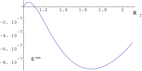
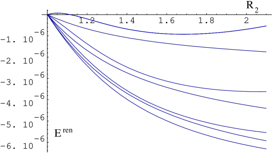
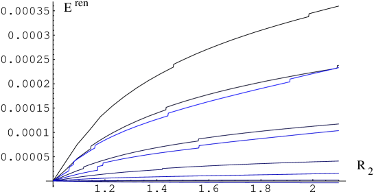
6.2 Magnetic string

6.2.1 Finite and asymptotic vacuum energy

1. Finite energy

The finite part of the ground state energy, $E_{f}$, is used in the form as given by Eq. (5.225). Let $E_{f}(\nu,k)$ denote the function to be integrated and summed over in that expression. In Fig.17 it is shown as function of $k$ for several values of the orbital momentum $\nu$. In order the make the behaviour better visible it is multiplied there by $\nu^{4}k^{3}$. These functions are smooth for all values of $k$, starting from some finite values at $k=0$.

Figure 15: for $R_{1}=0.0001,R_{2}=1.,\ \Omega=3.$ the bundle of $-\frac{1}{\pi}k\ln f_{\nu}^{sub}(ik);\frac{1}{2}<\nu<250\frac{1}{2}$, multiplied with $k^{2}$

Figure 16: Contribution of each integral $-\frac{1}{\pi}\int\limits_{m}^{\infty}k\ln f_{\nu}^{sub}(ik)dk$ (multiplied with $\nu^{2}$

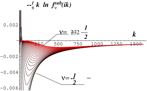
For large $k$, the functions $\nu^{4}k^{2}E_{f}(\nu,k)$ shown here tend to a constant thus the integral over $k$ is convergent. All integrals have been truncated at $k=1500$. The error caused by this is quite small and does not change the results shown in the Table II. These integrals we denote by $E_{f}(\nu)$. They are shown as function of $\nu$ in Fig.18 in a logarithmic scale. Again, we multiplied by a power of argument, here by $\nu^{2}$, in order to make the behaviour for large $\nu$ visible. It is seen that $\nu^{2}E_{f}(\nu)$ tends to a constant so that the sum over $\nu$ is convergent. The sum is taken up to $\nu=232.5$ and again the remainder is small.

Figure 17: The contribution $E_{f}(\nu,k)$ multiplied by $\nu^{4}k^{3}$ of the individual radial momenta for several orbital momenta to the finite part of the ground state energy for $R_{1}=0.0001$, $R_{2}=1$, $\Omega=3$.

Figure 18: The contribution $E_{f}(\nu)$ of the individual orbital momenta to the finite part of the ground state energy multiplied by $\nu^{2}$ for $R_{1}=0.0001$,$R_{2}=1$ and $\Omega=3$.

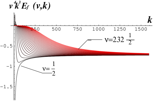
The calculations have been performed for several values of the parameters. The results are displayed in Table.II. The computations are performed with an adapted arithmetical precision. In intermediate steps compensations between sometimes very large quantities appeared. The precision was adapted accordingly. For example, for $R_{1}=0.99,\nu=250.5,k=1600$ as much as 1404 decimal positions have been necessary to get at least 16 digits precision of the integrand $E_{f}(\nu,k)$. This was a factor causing large computation time.

2. Asymptotic energy

The asymptotic part of the ground state energy as given by Eqs.(5.235) together with (8.63) can be represented as sum of a part proportional to the second power of the flux and one proportional to the fourth power,

$$E^{as}=-\frac{4}{\pi}[e_{1}(R_{1},R_{2})\Omega^{2}+e_{2}(R_{1},R_{2})\Omega^{4}].$$ (6.2)

The corresponding coefficients $e_{1}(R_{1},R_{2})$ and $e_{2}(R_{1},R_{2})$ can be calculated numerically without problems. They are shown as functions of $R_{2}$ for fixed $R_{1}$ in Fig.19 (multiplied by $R_{2}^{2}$).

Figure 19: The asymptotic part of energy as function of the outer radius for $R_{1}=0.00001$ and $R_{1}=1$ resp.

6.2.2 Parametrical dependence of vacuum energy

Table II The numerical evaluations for several values of $R_{1}$ and $\Omega$

$R_{1}$=0.0001
$\Omega$ $E^{f}$ $E^{as}$ $E^{ren}$ $E^{class}$ $E^{tot}$ 0.5 -0.0130152 0.00152886 -0.0114863 3.14159 3.13011 1. -0.052403 0.00509591 -0.0473071 12.5664 12.5191 3. -0.450093 -0.052012 -0.502105 113.097 112.595 6. -0.91953 -1.52936 -2.44889 452.389 449.94 10. 4.85954 -12.9483 -8.08871 1256.64 1248.55 15. 46.3333 -67.3661 -21.0328 2827.43 2806.4 21. 215.273 -261.526 -46.2534 5541.77 5495.52 30. 987.62 -1095.29 -107.666 11309.7 11202.1

$R_{1}$=0.9
$\Omega$ $E^{f}$ $E^{as}$ $E^{ren}$ $E^{class}$ $E^{tot}$ 0.5 -0.278679 -0.00105651 -0.279736 16.5347 16.255 1. -1.11431 -0.00451479 -1.11882 66.1388 65.02 3. -10.0633 -0.0683525 -10.1317 595.249 585.117 6. -40.4372 -0.647622 -41.0848 2381. 2339.92 10. -112.17 -4.2629 -116.433 6613.88 6497.45 20. -423.279 -63.2506 -486.53 26455.5 25969. 40. -1079.05 -992.187 -2071.24 105822. 103751.

$R_{1}$=0.95
$\Omega$ $E^{f}$ $E^{as}$ $E^{ren}$ $E^{class}$ $E^{tot}$ 0.5 -0.72166 -0.00212769 -0.723788 32.2215 31.4977 1. -2.86633 -0.00877711 -2.87511 128.886 126.011 3. -25.8293 -0.104564 -25.9339 1159.97 1134.04 10. -287.834 -4.39364 -292.228 12888.6 12596.4

$R_{1}$=0.99
$\Omega$ $E^{f}$ $E^{as}$ $E^{ren}$ $E^{class}$ $E^{tot}$ 0.5 -5.59211 -0.0106385 -5.60275 157.869 152.266 1. -23.2975 -0.0428038 -23.3403 631.476 608.136 3. -202.057 -0.409235 -202.466 5683.28 5480.82

$R_{1}$=0.997
$\Omega$ $E^{f}$ $E^{as}$ $E^{ren}$ $E^{class}$ $E^{tot}$ 1. -91.996 -0.142036 -92.138 2097.54 2005.4

$R_{1}$=0.999
$\Omega$ $E^{f}$ $E^{as}$ $E^{ren}$ $E^{class}$ $E^{tot}$ 1. -311.182 -0.425555 -311.608 6286.33 5974.72

The results are displayed mainly in Table II. For small inner radius of the flux the results are close to them of [19] where the same problem for a flux tube with homogeneous magnetic field inside, which corresponds to $R_{1}=0$ here, was considered. Especially, it is seen that for large flux $\Omega$ there is a compensation of the $\Omega^{4}$-contribution between the finite and the asymptotic parts of the ground state energy leaving a behaviour proportional to $\Omega^{2}\ln\Omega$ as shown in Fig.20. Here the asymptotic part gave an essential contribution. The ground state energy remains negative, but numerically small. Only for very large flux it could overturn the corresponding classical energy, but these values of the flux are clearly unphysical.

Figure 20: The ground state energy divided by $\Omega^{2}\ln\Omega$ as function of $\Omega$.

For values of the inner radius close to the outer one, $R_{1}\to 1$ (where we have put $R_{2}=1$) the picture changes. Here the vacuum energy grows faster than the classical one. Generally, both diverge proportional to $(1-R_{1})^{-1}$, the classical energy is equal to $E_{\rm class}=\Omega^{2}2\pi(1-R_{1})^{-1}$. The vacuum energy, multiplied by $(1-R_{1})$, is shown in Fig.21 in a logarithmic scale. It is negative and growing a bit faster than the classical one which would be a constant in this plot. Here the asymptotic part of the ground state energy becomes increasingly unimportant (see Table II).

6.2.3 Some remarks on the numerical difficulties

The calculations have been performed for several values of the parameters. The results for magnetic string are displayed in Table.1. The computations are performed with an adapted arithmetical precision. In intermediate steps compensations between sometimes very large quantities appeared. The precision was adapted accordingly. For example, for $R_{1}=0.99,\nu=250.5,k=1600$ as much as 1404 decimal positions have been necessary to get at least 16 digits precision of the integrand $E_{f}(\nu,k)$. This was a factor causing large computation time.

6.3 NO vortex

We investigated numerically the vacuum energy for values of $\beta$ ranging from $\beta=0.3$ to $\beta=6$ for some choices of the parameters $f_{e}$ and $\eta$. The results are represented in Table III. In the Figs. 21 and 22 two examples for the dependence of the individual parts of the vacuum energy on the parameter $\beta$ are displayed.

Figure 21: The vacuum energy as a function of $\beta$ for the $q=0.5$, $f_{e}=1$, $\eta=1$. In order to represent all quantities within one plot the classical energy is divided by 200.

Figure 22: The same as in figure 21 but for $q=2$.

The constituent parts of the vacuum energy
Table III $q$ $\beta$ $f_{e}$ $\eta$ $E_{\rm class}$ ${\cal E}^{\rm as}$ ${\cal E}^{\rm f}$ ${\cal E}_{\rm ren}={\cal E}^{\rm as}+{\cal E}^{\rm f}$ 0.5 0.3 1 1 3.902 -0.006102 0.02410 0.01800 0.5 0.6 1 1 4.549 -0.006102 0.01590 0.009795 0.5 1. 1 1 5.099 -0.006104 0.01153 0.005421 0.5 3.5 1 1 6.710 -0.006146 0.004224 -0.001922 0.5 6. 1 1 7.507 -0.006208 0.001884 -0.004325 2. 0.3 1 1 2.105 -0.003170 -0.001883 -0.005053 2. 0.6 1 1 2.399 -0.002891 -0.007285 -0.01018 2. 1. 1 1 2.652 -0.002924 -0.01182 -0.01475 2. 3.5 1 1 2.652 -0.002924 -0.02451 -0.02743 2. 6. 1 1 3.861 -0.006539 -0.03022 -0.03676 0.5 0.3 0.1 0.1 0.03902 -0.00006102 -9.589 $10^{-6}$ -0.00007061 0.5 0.6 0.1 0.1 0.04549 -0.00006102 -0.00001214 -0.00007316 0.5 1. 0.1 0.1 0.05099 -0.00006104 -0.00001421 -0.00007525 0.5 3.5 0.1 0.1 0.06710 -0.00006146 -0.00001975 -0.00008121 0.5 6. 0.1 0.1 0.07507 -0.00006208 -0.00002216 -0.00008425

The vacuum energy $E^{ren}$ decreases for large values of the vortex parameter $\beta$. The contribution of $E^{ren}$ to the total energy of vortex can be positive as well as negative, dependent on the magnitude of the electric charge $q$. Nevertheless it remains sufficiently smaller compared to the classical energy $E_{class}$.

7 Conclusions and Discussions

In the preceding sections the ground state energy for a spinor quantum field in the background of a rectangular shaped magnetic flux and of the Nielsen-Olesen vortex, and for a scalar field in the rectangular scalar background has been calculated.

The used regularization procedure is a kind of zeta functional regularization . The sum over spectrum of hamiltonian is performed in terms of the Jost function for the corresponding scattering problem.

The Jost function for each model has been written down explicitly, also its asymptotic part as well. The numerical calculation for several models (spinor field) required work with high arithmetic precision. The obtained results presume some discussion

7.1 Scalar field in scalar background.

This model is the simplest construction which allows to carry out analytic calculations as well as numeric evaluations relative easy.

The regularization procedure with the renormalization of the ground state energy and its interpretation is also quite transparent. Nevertheless this model looks up a number of interesting results concerning the behaviour of the vacuum energy. The vacuum energy can provide positive as well as negative contributions to the total energy. The sign of it depends on the magnitude of the background potential $V$. Moreover, there is a thin range of values $V$, whereat the ground state energy shows the critical behaviour for its dependence on the outer radius $R_{2}$ possessing one maximum and one minimum. It gives reason to suppose an existence of stable states of the scalar string, generated by the vacuum corrections.

7.2 Spinor field in magnetic background.

The spinor vacuum energy for the constructed magnetic string is investigated for several values of potential $\Omega$ and inner radius $R_{1}$. It shows no extrema, so the magnetic string constructing in such a way must be unstable. The known asymptotic behaviour of the one one-loop vacuum energy for large magnitude of background potential in the form $\Omega^{2}\ln\Omega$ is also confirmed fro this model.

The question whether the vacuum energy for sufficiently small thickness of magnetic flux may become larger than the classical one cannot be answered by the numerical results obtained. The problem is that the computations become very time consuming because of the increasing precision which is required. Also, one has to take higher $k$ and $\nu$ into account. The weakening of the growth for $R_{1}=0.997$ and $R_{1}=0.999$ (while $R_{2}$ is fixed to be equal 1) seen in Fig.21 may be caused just by this reason. Here one has to note that the integrand is for large $k$ and $\nu$ always negative (see Fig.17) so that dropping some part (as we did within the numerical procedure) diminishes the result. So, as a result, we cannot exclude from the given calculation that the vacuum energy grows for a strong background field faster than the classical energy.

Figure 23: The vacuum energy multiplied by $(1-R_{1})$ in a logarithmic scale for $\Omega=1$.

Further work is necessary to better understand these questions. An improvement of the numerical procedure is certainly desirable. It could go along two lines. First, in the calculation of the Jost function the compensation of large exponentials should be avoided by taking them into account analytically. Second, in the compensation between the logarithm of the Jost function and its asymptotic expansion in the integrand of $E_{f}$ in Eq.(5.225) higher orders of the asymptotic expansion could be used. However, for this reason one would have to continue the procedure invented in [19] for this expansion using the Lippmann-Schwinger equation or to find some equivalent procedure.

7.3 Spinor field in NO vortex background.

During the analytical regularization of the ground state energy in the model with the special interaction term is occurred. Namely the standard zeta functional regularization determines the counter terms from the first heat kernel coefficients (up to $a_{2}$). It turned out that to renormalize the vacuum energy one has to introduce a counter term which is not present in the initial action and represents a non polynomial interaction. This is caused by the non polynomial interaction present in the model itself Sec.(3).

In the considered case the background is given purely numerically. This is the crucial technical difference to the previous two models where it allowed an analytically calculation. However, it has been demonstrated that the similar computational scheme used here is able to work successfully with such backgrounds. This is a step forward to physically really interesting problems. In the considered model the stability of the background is given by topological arguments and for a realistic choice of the parameters the quantum contribution is small. This smallness has two sources. The one is the smallness of the coupling constants which appears in front of the quantum contribution relative to the classical one. The second one is a purely numerical smallness of about two orders of magnitude. It is present even if the parameters and couplings are all of order one, see for instance the Fig.21.

As seen from the table and from the Figs.21 and 22, for the dependence of the vacuum energy on the various parameters no general rule can be seen so far. Even the sign of the vacuum energy changes. The same applies to the relative weight of the individual contributions. Sometimes the asymptotic part is dominating, in other cases, however, the ’finite’ part is larger. In general, they are of the same order. From this one can conclude only that in the given background there is no small parameter which could allow for some approximation scheme. For instance, if the asymptotic part is dominating one could hope to get a good approximation by including higher orders of the uniform asymptotic expansion of the Jost function into the asymptotic part of the vacuum energy and neglect the ’finite’ part of it which is the numerically much harder part of the problem. The examples in [13] have been a kind of suggesting this way in contrast to the example in the present paper.

For the considered model of a spinor in the background of the NO vortex, the vacuum energy due to its smallness has only a very negligible influence on the dynamics of the background. Hence in the considered case the vacuum energy is of limited physical importance. However, its calculation gave new insights into the structure of such calculations and demonstrated the power of the methods used. A next step could be to apply them to the $Z$ and electroweak strings where the stability is not guaranteed by topological arguments and where the stability issue is not finally settled with respect to the fermion contributions [2, 51].

7.4 Summary

Basically, the contribution of the quantum ground state has an influence on the macroscopic behaviour of the field system. The degree of this influence depends on the nature of the interacting background and fluctuations as well as on the kind of interaction and coupling parameters. The vacuum corrections can provide both negative and positive contributions to the total energy.

It has been shown for scalar and magnetic strings with a simple rectangular shape and for the NO vortex.

In all three cases the general dependence of the vacuum contributions on the background properties is not to be formulated certainly.

For the scalar string, even the alternation of the stability properties is possible. The large-potential asymptotics known for homogeneous fields is confirmed for scalar and spinor strings.

In the technical aspect, the known methods using the zeta functional regularization and heat kernel expansion have been applied successfully to more complicated shapes of backgrounds as before, and in particular to the shape being given pure numerically (NO-vortex).

The obtained results suggest the applicability of the developed methods and technics to calculations of the vacuum energy in more complicated background configurations, such as monopoles, electroweak strings, skyrmions, sphalerons etc.

These future investigations would lead to better understanding of the phenomena of vacuum energy and its relation to the geometry of classical backgrounds.

8 Appendix

8.1 The uniform asymptotic expansions for logarithm of Jost function

8.1.1 The uniform asymptotics of modified Bessel functions
K and I

The uniform asymptotic expansion of modified Bessel functions $K_{\nu\pm\frac{1}{2}}(kr),I_{\nu\pm\frac{1}{2}}(kr)$ in the combined limit $\nu,k\rightarrow\infty,\ k/\nu\equiv z=const$, can be obtained as series of the variable $t=1/\sqrt{1+z^{2}r^{2}}$ [1]:

$$K_{\nu+\frac{1}{2}}(\nu z\ r)\sim\sqrt{\frac{\pi}{2\nu}}\exp\{\sum\limits_{i=-1}^{\infty}\frac{S_{i}^{-}[\frac{1}{2},t]}{\nu^{i}}\}\equiv\sqrt{\frac{\pi}{2\nu}}e^{-\nu\eta}\sqrt{t}\left(\frac{1+t}{1-t}\right)^{1/4}\exp\{\sum\limits_{i=1}^{\infty}\frac{S_{i}^{-}[\alpha,t]}{\nu^{i}}\}$$

$$K_{\nu-\frac{1}{2}}(\nu z\ r)\sim\sqrt{\frac{\pi}{2\nu}}\exp\{\sum\limits_{i=-1}^{\infty}\frac{S_{i}^{-}[-\frac{1}{2},t]}{\nu^{i}}\}\equiv\sqrt{\frac{\pi}{2\nu}}e^{-\nu\eta}\sqrt{t}\left(\frac{1-t}{1+t}\right)^{1/4}\exp\{\sum\limits_{i=1}^{\infty}\frac{S_{i}^{-}[\alpha,t]}{\nu^{i}}\}$$

$$I_{\nu+\frac{1}{2}}(\nu z\ r)\sim\sqrt{\frac{1}{2\pi\nu}}\exp\{\sum\limits_{i=-1}^{\infty}\frac{S_{i}^{-}[\frac{1}{2},t]}{\nu^{i}}\}\equiv\sqrt{\frac{1}{2\pi\nu}}e^{\nu\eta}\sqrt{t}\left(\frac{1-t}{1+t}\right)^{1/4}\exp\{\sum\limits_{i=1}^{\infty}\frac{S_{i}^{+}[\alpha,t]}{\nu^{i}}\}$$

$$I_{\nu-\frac{1}{2}}(\nu z\ r)\sim\sqrt{\frac{1}{2\pi\nu}}\exp\{\sum\limits_{i=-1}^{\infty}\frac{S_{i}^{-}[-\frac{1}{2},t]}{\nu^{i}}\}\equiv\sqrt{\frac{1}{2\pi\nu}}e^{\nu\eta}\sqrt{t}\left(\frac{1+t}{1-t}\right)^{1/4}\exp\{\sum\limits_{i=1}^{\infty}\frac{S_{i}^{+}[\alpha,t]}{\nu^{i}}\}$$

where $S_{i}^{\pm}[\alpha,t]$ are:
for $K_{\nu+\alpha}$, $\alpha=\pm\frac{1}{2}$ :

$$S_{-1}^{-}[t,\alpha]=-\frac{1}{t}-\frac{1}{2}\ln\frac{1-t}{1+t}$$

$$S_{0}^{-}[t,\alpha]=\frac{\ln t}{2}+\frac{\alpha}{2}\ln\frac{1+t}{1-t}$$

$$S_{1}^{-}[t,\alpha]=\frac{t}{24}(-3+12\alpha^{2}-12\alpha t+5t^{2})$$

$$S_{2}^{-}[t,\alpha]=\frac{1}{48}t^{2}\left[-8\alpha^{3}t+12\alpha^{2}(-1+2t^{2})+\alpha(26t-30t^{3})+3(1-6t^{2}+5t^{4})\right]$$

$$S_{3}^{-}[t,\alpha]=\frac{1}{5760}\left\{t^{3}\left[-375+4779t^{2}-9945t^{4}+5525t^{6}+240\alpha^{4}(3t^{2}-1)-\right.\right.$$

$$\left.\left.960\alpha^{3}t(4t^{2}-3)-720\alpha t(7-22t^{2}+15t^{4})-120\alpha^{2}(13-84t^{2}+75t^{4})\right]\right\}$$

$$S_{4}^{-}[t,\alpha]=$$

$$\frac{1}{1920}\left\{t^{4}\left[-48\alpha^{5}t(5t^{2}-3)+240\alpha^{4}(1-8t^{2}+8t^{4})-40\alpha^{3}t(69-240t^{2}+175t^{4})+\right.\right.$$

$$\left.\left.120\alpha^{2}(-7+94t^{2}-207t^{4}+120t^{6})+\alpha(3561t-21225t^{3}-342255t^{5}-16575t^{7})\right.\right.$$

$$\left.\left.+15(13-284t^{2}+1062t^{4}-1356t^{6}+565t^{8})\right]\right\}$$ (8.1)

for $I_{\nu+\alpha}$, $\alpha=\pm\frac{1}{2}$ :

$$S_{-1}^{+}[t,\alpha]=\frac{1}{t}+\frac{1}{2}\ln\frac{1-t}{1+t}$$

$$S_{0}^{+}[t,\alpha]=\frac{\ln t}{2}-\frac{\alpha}{2}\ln\frac{1+t}{1-t}$$

$$S_{1}^{+}[t,\alpha]=-\frac{t}{24}(-3+12\alpha^{2}+12\alpha t+5t^{2})$$

$$S_{2}^{+}[t,\alpha]=\frac{1}{48}t^{2}\left[8\alpha^{3}t+12\alpha^{2}(-1+2t^{2})+\alpha(-26t+30t^{3})+3(1-6t^{2}+5t^{4})\right]$$

$$S_{3}^{+}[t,\alpha]=-\frac{1}{5760}\left\{t^{3}\left[-375+4779t^{2}-9945t^{4}+5525t^{6}+240\alpha^{4}(3t^{2}-1)+\right.\right.$$

$$\left.\left.960\alpha^{3}t(4t^{2}-3)+720\alpha t(7-22t^{2}+15t^{4})+120\alpha^{2}(13-84t^{2}+75t^{4})\right]\right\}$$

$$S_{4}^{+}[t,\alpha]=$$

$$\frac{1}{1920}\left\{t^{4}\left[48\alpha^{5}t(5t^{2}-3)+240\alpha^{4}(1-8t^{2}+8t^{4})+40\alpha^{3}t(69-240t^{2}+175t^{4})+\right.\right.$$

$$\left.\left.120\alpha^{2}(-7+94t^{2}-207t^{4}+120t^{6})-\alpha(3561t-21225t^{3}-342255t^{5}-16575t^{7})\right.\right.$$

$$\left.\left.+15(13-284t^{2}+1062t^{4}-1356t^{6}+565t^{8})\right]\right\},$$ (8.2)

what leads in particular to

$$\eta\equiv\eta(t)=\frac{1}{t}+\ln\frac{1-t}{1+t}$$ (8.3)

in (8.1.1, 8.1)

8.1.2 The saddle point expansion

The evaluation of integrals of type

$$\int\limits_{0}^{r}e^{\nu\eta(r^{\prime})}\phi(r^{\prime})dr^{\prime},$$ (8.4)

entering in the expressions of $\ln f_{\nu}^{(n)}$ Sec.5.3 (5.145) has been done by using the saddle point approach (See. for example [70]). The derivation is described in details in [20]. We use the results given in App.[19] as a starting point:

$$\int\limits_{0}^{r}e^{\nu\eta(r^{\prime})}\phi(r^{\prime})dr^{\prime}=e^{\nu\eta(r)}\sum\limits_{k=1}^{\infty}h_{k-1}\nu^{-k}$$ (8.5)

with the first several coefficients of the expansion

$$h_{0}=\frac{\phi(r)}{\eta^{\prime}(r)},\ \ \ \ \ \ \ \ h_{1}=\frac{\phi(r)\eta^{\prime\prime}(r)}{\eta^{\prime}(r)^{3}}-\frac{\phi^{\prime}(r)}{\eta^{\prime}(r)^{2}}$$

$$h_{2}=\frac{\phi^{\prime\prime}(r)}{\eta^{\prime}(r)^{3}}-\frac{3\phi^{\prime}(r)\eta^{\prime\prime}(r)}{\eta^{\prime}(r)^{4}}+\frac{3\phi(r)\eta^{\prime\prime}(r)^{2}}{\eta^{\prime}(r)^{5}}-\frac{\phi(r)\eta^{\prime\prime\prime}(r)}{\eta^{\prime}(r)^{4}}$$ (8.6)

8.1.3 Scalar field with scalar background

We proceed from the expansion of the logarithmic Jost function Sec.5.3 (5.145) obtained by iterations of the Lippmann-Schwinger equation (5.142).

The terms $\ln f_{l}^{(1)}(ik)$ are obtained as described in Sec.5.3 by substitution of (5.3.2) in (5.141):

$$\ln f_{l}^{(1)}(ik)=\int\limits_{0}^{\infty}rdrV(r)K_{l}(kr)I_{l}(kr)$$

$$\ln f_{l}^{(2)}(ik)=\int\limits_{0}^{\infty}rdrV(r)K_{l}(kr)\int_{0}^{r}r^{\prime}dr^{\prime}V(r^{\prime})\left[I_{l}(kr)K_{l}(kr^{\prime})-I_{l}(kr^{\prime})K_{l}(kr)\right]I_{l}(kr^{\prime})-$$

$$\frac{1}{2}\int\limits_{0}^{\infty}rdrV(r)K_{l}(kr)I_{l}(kr)\int\limits_{0}^{\infty}r^{\prime}dr^{\prime}V(r^{\prime})K_{l}(kr^{\prime})I_{l}(kr^{\prime})$$

$$\ln f_{l}^{(3)}(ik)=\int\limits_{0}^{\infty}rdrV(r)K_{l}(kr)\int_{0}^{r}r^{\prime}dr^{\prime}V(r^{\prime})\left[I_{l}(kr)K_{l}(kr^{\prime})-I_{l}(kr^{\prime})K_{l}(kr)\right]\times$$

$$\times\left(\int\limits_{0}^{r^{\prime}}r^{\prime\prime}dr^{\prime\prime}V(r^{\prime\prime})I_{l}(kr^{\prime})K_{l}(kr^{\prime\prime})I_{l}(kr^{\prime\prime})-\int\limits_{0}^{r^{\prime}}r^{\prime\prime}dr^{\prime\prime}V(r^{\prime\prime})K_{l}(kr^{\prime})I_{l}(kr^{\prime\prime})^{2}\right)$$

$$-\frac{1}{2}\left(\int\limits_{0}^{\infty}rdrV(r)K_{l}(kr)I_{l}(kr)\int\limits_{0}^{\infty}r^{\prime}dr^{\prime}V(r^{\prime})K_{l}(kr^{\prime})\int\limits_{0}^{r^{\prime}}r^{\prime\prime}dr^{\prime\prime}V(r^{\prime\prime})[I_{l}(kr^{\prime})K_{l}(kr^{\prime\prime})-\right.$$

$$\left.\hskip 142.26378ptI_{l}(kr^{\prime\prime})K_{l}(kr^{\prime})]I_{l}(kr^{\prime\prime})+\right.$$

$$\left.\int\limits_{0}^{\infty}rdrV(r)K_{l}(kr)\int\limits_{0}^{r}V(r^{\prime})[I_{l}(kr)K_{l}(kr^{\prime})-I_{l}(kr^{\prime})K_{l}(kr)]I_{l}(kr^{\prime})\times\right.$$

$$\left.\hskip 113.81102pt\int\limits_{0}^{\infty}r^{\prime\prime}dr^{\prime\prime}V(r^{\prime\prime})K_{l}(kr^{\prime\prime})I_{l}(kr^{\prime\prime})\right)+$$ (8.7)

$$\frac{1}{3}\int\limits_{0}^{\infty}rdrV(r)K_{l}(kr)I_{l}(kr)\int\limits_{0}^{\infty}r^{\prime}dr^{\prime}V(r^{\prime})K_{l}(kr^{\prime})I_{l}(kr^{\prime})\int\limits_{0}^{\infty}r^{\prime\prime}dr^{\prime\prime}V(r^{\prime\prime})K_{l}(kr^{\prime\prime})I_{l}(kr^{\prime\prime})$$

The expression $\ln f_{l}^{(1)}(ik)$ has already a usable form and $\ln f_{l}^{(2-3)}(ik)$ can be simplified if we use its symmetry properties in respect of the change $r\leftrightarrow r^{\prime}$.

The procedure is illustrated by the $\ln f_{l}^{(2)}(ik)$. We start with the expression (8.1.3)

$$\ln f_{l}^{(2)}(ik)=$$

$$\int\limits_{0}^{\infty}rdrV(r)K_{l}(kr)I_{l}(kr)\int_{0}^{r}r^{\prime}dr^{\prime}V(r^{\prime})K_{l}(kr^{\prime})I_{l}(kr^{\prime})-$$

$$\int\limits_{0}^{\infty}rdrV(r)K_{l}(kr)K_{l}(kr)\int_{0}^{r}r^{\prime}dr^{\prime}V(r^{\prime})I_{l}(kr^{\prime})I_{l}(kr^{\prime})$$

$$-\frac{1}{2}\int\limits_{0}^{\infty}rdrV(r)K_{l}(kr)I_{l}(kr)\int\limits_{0}^{\infty}r^{\prime}dr^{\prime}V(r^{\prime})K_{l}(kr^{\prime})I_{l}(kr^{\prime}).$$

Then we represent the last term as

$$\frac{1}{2}\int\limits_{0}^{\infty}rdrV(r)K_{l}(kr)I_{l}(kr)\int\limits_{0}^{\infty}r^{\prime}dr^{\prime}V(r^{\prime})K_{l}(kr^{\prime})I_{l}(kr^{\prime})=$$

$$\frac{1}{2}\int\limits_{0}^{\infty}rdrV(r)K_{l}(kr)I_{l}(kr)\left[\int\limits_{0}^{r}+\int\limits_{r}^{\infty}\right]r^{\prime}dr^{\prime}V(r^{\prime})K_{l}(kr^{\prime})I_{l}(kr^{\prime}),$$

and take into account the rule of change the integration order:

$$\int\limits_{0}^{\infty}f(r)dr\int\limits_{0}^{r}g(r^{\prime})dr^{\prime}\equiv\int\limits_{0}^{\infty}g(r)dr\int\limits_{r}^{\infty}f(r^{\prime})dr^{\prime},$$ (8.8)

which allows to see, that the last term is equal exactly to the first one but with the sign minus in front of them. Thus these terms cancel each other, and we have:

$$\ln f_{l}^{(2)}(ik)=-\int\limits_{0}^{\infty}rdrV(r)K_{l}(kr)K_{l}(kr)\int_{0}^{r}r^{\prime}dr^{\prime}V(r^{\prime})I_{l}(kr^{\prime})I_{l}(kr^{\prime}).$$ (8.9)

We do not discuss here the simplification of $\ln f_{l}^{(3)}(ik)$, because it is not needed for minimal subtraction, as pointed out in Sec. 5.3.

Since the contribution of $l=0$ in the sum over $l$ in (5.220, 5.221, 5.222) Sec.5.4, is separated, the $\ln f_{0}(ik)$ is to perform additionaly. Instead of the uniform asymptotic expansion (because $l\equiv 0\equiv const$) the usual asymptotics at $k\rightarrow\infty$ is used.

We use entirely the corresponding asymptotics of modified Bessel functions

$$I_{0}(z)\sim\frac{e^{z}}{\sqrt{2\pi z}}\left\{1+\frac{1}{8z}+\frac{9}{2(8z)^{2}}+\dots\right\}$$

$$K_{0}(z)\sim e^{-z}\sqrt{\frac{\pi}{2z}}\left\{1-\frac{1}{8z}+\frac{9}{2(8z)^{2}}+\dots\right\},$$ (8.10)

which are to substitute into (5.139-5.145,Sec.5.3) with the argument $z$ having the values $kR_{1},kR_{2},qR_{1},qR_{2}$.

Recall, that $q=\sqrt{k^{2}+V_{0}}$, that provides in the considered limit $k\rightarrow\infty$

$$q\sim k+\frac{V_{0}}{2k}-\frac{V_{0}^{2}}{4k^{3}}+O(k^{-4}).$$ (8.11)

Substituted into (5.2.1) it provides the leading order for $\ln f_{0}^{as}(ik)$:

$$\ln f_{0}^{as}(ik)\sim-\frac{V_{0}}{2k}(R_{1}-R_{2}).$$ (8.12)

8.1.4 Spinor field with magnetic background

( To 5.6, Higher orders of the Jost function )

The asymptotic of the logarithmic Jost function can be obtained in the form: $\ln f_{\nu}(ik)=\sum\limits_{n}h_{n}(t_{1},t_{2})$,(see 5.261) with:

$$h_{1} = \frac{4}{3}\lambda^{2}[{R_{1}}^{4}t_{1}(2+t_{1}){(1+t_{2})}^{2}-3{R_{1}}^{2}{R_{2}}^{2}{(1+t_{1})}^{2}t_{2}(1+t_{2})+{R_{2}}^{4}{(1+t_{1})}^{2}t_{2}(1+2t_{2})]$$

$$h_{2} = 0$$

$$h_{3} = -\frac{1}{6}{\lambda}^{2}[2{R_{1}}^{4}{t_{1}}^{3}{(1+t_{2})}^{2}+{R_{1}}^{2}{R_{2}}^{2}{(1+t_{1})}^{2}{t_{2}}^{3}{(1+t_{2})}^{2}(3{t_{2}}^{2}-4)-$$

$${R_{2}}^{4}{(1+t_{1})}^{2}{t_{2}}^{3}(3{t_{2}}^{4}+6{t_{2}}^{3}-{t_{2}}^{2}-8t_{2}-2)]+$$

$$\frac{2}{15}{\lambda}^{4}[4{R_{1}}^{8}{t_{1}}^{3}(4+t_{1}){(1+t_{2})}^{4}-5{R_{1}}^{6}{R_{2}}^{2}{(1+t_{1})}^{4}{t_{2}}^{3}{(1+t_{2})}^{4}+$$

$$15{R_{1}}^{4}{R_{2}}^{4}{(1+t_{1})}^{4}{t_{2}}^{3}{(1+t_{2})}^{2}({t_{2}}^{2}+2t_{2}-1)-$$

$$5{R_{1}}^{2}{R_{2}}^{6}{(1+t_{1})}^{4}{t_{2}}^{3}(3{t_{2}}^{4}+12{t_{2}}^{3}+6{t_{2}}^{2}-4t_{2}-1)+$$

$${R_{2}}^{8}{(1+t_{1})}^{4}{t_{2}}^{3}(5{t_{2}}^{4}+20{t_{2}}^{3}-4t_{2}-1)]$$

$$h_{4} = \frac{\delta^{2}[{R_{1}}^{4}{t_{1}}^{4}(1-{t_{1}}^{2})+{R_{2}}^{4}{t_{2}}^{4}(1-{t_{2}}^{2})]}{4{(R_{1}^{2}-R_{2}^{2})}^{2}}$$

$$\lambda = \frac{\delta}{(R_{1}^{2}-R_{2}^{2})(1+t_{1})(1+t_{2})}$$ (8.13)

8.1.5 Spinor field with NO vortex background

Uniform asymptotics for Jost function in abelian Higgs Background We start with the expansion (5.145) obtained in [20] in the form

$$\ln f^{(1)}_{\nu}(k) = \left(\frac{\pi}{2i}\right)\int\limits_{0}^{\infty}dr\ r\ \Phi^{0\ T}_{H}(r)\hat{V}(r)\Phi^{0}_{J}(r),$$ (8.14)

$$\ln f^{(2)}_{\nu}(k) = -\left(\frac{\pi}{2i}\right)^{2}\int\limits_{0}^{\infty}dr\ r\ \int\limits_{0}^{r}dr^{\prime}\ r^{\prime}\ \Phi^{0\ T}_{H}(r)\hat{V}(r)\Phi^{0}_{H}(r)\$$ (8.15)

$$\hskip 28.45274pt\times\Phi^{0\ T}_{J}(r^{\prime})\hat{V}(r^{\prime})\Phi^{0}_{J}(r^{\prime}),$$

$$\ln f^{(3)}_{\nu}(k) = 2\left(\frac{\pi}{2i}\right)^{3}\int\limits_{0}^{\infty}dr\ r\ \int\limits_{0}^{r}dr^{\prime}\ r^{\prime}\ \int\limits_{0}^{r^{\prime}}dr^{\prime\prime}\ r^{\prime\prime}\ \Phi^{0\ T}_{H}(r)\hat{V}(r)\Phi^{0}_{H}(r)\$$ (8.16)

$$\hskip 28.45274pt\times\Phi^{0\ T}_{H}(r^{\prime})\hat{V}(r^{\prime})\Phi^{0}_{J}(r^{\prime})\Phi^{0\ T}_{J}(r^{\prime\prime})\hat{V}(r^{\prime\prime})\Phi^{0}_{J}(r^{\prime\prime}),$$

$$\ln f^{(4)}_{\nu}(k) = -\left(\frac{\pi}{2i}\right)^{4}\int\limits_{0}^{\infty}dr\ r\ \int\limits_{0}^{r}dr^{\prime}\ r^{\prime}\ \int\limits_{0}^{r^{\prime}}dr^{\prime\prime}\ r^{\prime\prime}\ \int\limits_{0}^{r^{\prime\prime}}dr^{\prime\prime\prime}\ r^{\prime\prime\prime}\$$ (8.17)

$$\hskip 28.45274pt\times\left[(4\Phi^{0\ T}_{H}(r)\hat{V}(r)\Phi^{0}_{H}(r)\ \Phi^{0\ T}_{H}(r^{\prime})\hat{V}(r^{\prime})\Phi^{0}_{J}(r^{\prime})\right.$$

$$\hskip 39.83368pt\Phi^{0\ T}_{H}(r^{\prime\prime})\hat{V}(r^{\prime\prime})\Phi^{0}_{J}(r^{\prime\prime})\Phi^{0\ T}_{J}(r^{\prime\prime\prime})\hat{V}(r^{\prime\prime\prime})\Phi^{0}_{J}(r^{\prime\prime\prime})$$

$$\hskip 39.83368pt+2\Phi^{0\ T}_{H}(r)\hat{V}(r)\Phi^{0}_{H}(r)\ \Phi^{0\ T}_{H}(r^{\prime})\hat{V}(r^{\prime})\Phi^{0}_{H}(r^{\prime})$$

$$\left.\hskip 39.83368pt\Phi^{0\ T}_{J}(r^{\prime\prime})\hat{V}(r^{\prime\prime})\Phi^{0}_{J}(r^{\prime\prime})\Phi^{0\ T}_{J}(r^{\prime\prime\prime})\hat{V}(r^{\prime\prime\prime})\Phi^{0}_{J}(r^{\prime\prime\prime})\right],$$

As a matter of fact we have to treat three kinds of products, entering in the integrals 5.179, namely

$$\Phi^{0\ T}_{H}(x)\hat{V}(x)\Phi^{0}_{H}(x),\ \ \Phi^{0\ T}_{J}(x)\hat{V}(x)\Phi^{0}_{J}(x),\ \ \Phi^{0\ T}_{H}(x)\hat{V}(x)\Phi^{0}_{J}(x),$$

and we denote them as ${\cal G}_{\{HVH\}}(x),\ {\cal G}_{\{JVJ\}}(x)$ and ${\cal G}_{\{HVJ\}}(x)$ for the first, second and third product respectively.

Performing the products (8.1.5) explicitly we obtain the expressions as follows:

$${\cal G}_{\{HVH\}}=\mu(r)(C^{-}H_{-}H_{-}-C^{+}H_{+}H_{+})-\frac{2v(r)}{r}\sqrt{C^{+}C^{-}}(H_{+}H_{-})$$ (8.18)

$${\cal G}_{\{JVJ\}}=\mu(r)(C^{-}J_{-}J_{-}-C^{+}J_{+}J_{+})-\frac{2v(r)}{r}\sqrt{C^{+}C^{-}}(J_{+}J_{-})$$ (8.19)

$${\cal G}_{\{HVJ\}}=\mu(r)(C^{-}H_{-}J_{-}-C^{+}H_{+}J_{+})-\frac{v(r)}{r}\sqrt{C^{+}C^{-}}(H_{+}J_{-}+H_{-}J_{+})$$

(8.20)

The notations has been used here are

$$C^{\pm}\equiv p_{0}\pm m_{0}$$

$$J_{\pm}\equiv J_{\nu\pm\frac{1}{2}}(q_{0}r)$$

$$H_{\pm}\equiv H^{(1)}_{\nu\pm\frac{1}{2}}(q_{0}r)$$

$$\sqrt{C^{+}C^{-}}\equiv\sqrt{p_{0}^{2}-m_{0}^{2}}$$

(8.21)

Recall that we have also to construct the Jost function of imaginary momentum $ik$. This procedure leads to substitution of Bessel functions by modified ones. As a result we have for the products defined by (8.20):

$${\cal G}_{\{HVH\}}\rightarrow{\cal G}_{\{KVK\}}\equiv ie^{-\pi\nu}\left(\frac{2}{i\pi}\right)^{2}\times$$

$$\left\{\tilde{\mu}[ip(K_{-}K_{-}+K_{+}K_{+})+m_{0}(K_{+}K_{+}-K_{-}K_{-})]-\frac{2v(r)}{r}\sqrt{p^{2}+m_{0}^{2}}K_{-}K_{+}\right\}$$

$${\cal G}_{\{JVJ\}}\rightarrow{\cal G}_{\{IVI\}}\equiv$$ (8.22)

$$\ \ \ \ \ -i\ e^{-\pi\nu}\left\{\tilde{\mu}[ip(I_{-}I_{-}+I_{+}I_{+})+m_{0}(I_{+}I_{+}-I_{-}I_{-})]+\frac{2v(r)}{r}\sqrt{p^{2}+m_{0}^{2}}I_{-}I_{+}\right\}$$

$${\cal G}_{\{HVJ\}}\rightarrow{\cal G}_{\{KVI\}}\equiv\frac{2}{i\pi}\times$$

$$\left\{\tilde{\mu}[ip(K_{-}I_{-}-K_{+}I_{+})-m_{0}(K_{-}I_{-}+K_{+}I_{+})]-\frac{v(r)}{r}\sqrt{p^{2}+m_{0}^{2}}(K_{+}I_{-}-K_{-}I_{+})\right\}$$

The notation of indices $\pm$ means as previous:

$$I_{\pm}\equiv I_{\nu\pm\frac{1}{2}}(qr)$$ (8.23)

$$K_{\pm}\equiv K_{\nu\pm\frac{1}{2}}(qr)$$ (8.24)

The substitution $k\rightarrow ik$ implies also the following redefinition of $q_{0},p_{0}$

$$k\rightarrow ik$$ (8.25)

$$p_{0}\rightarrow i\ p=i\ \sqrt{k^{2}-m_{e}^{2}}$$ (8.26)

$$q_{0}\rightarrow i\ q=i\ \sqrt{p^{2}+m_{0}^{2}}=i\ \sqrt{k^{2}-m_{e}^{2}+m_{0}^{2}}$$ (8.27)

respectively.

It can be seen from(8.1.5) that the Bessel functions which are to be integrated in (8.14-8.17) are ordered in products of pairs of kind

$$r\ K_{\pm}K_{\pm},\ r\ I_{\pm}I_{\pm},\ r\ K_{\pm}I_{\pm},\ r\ K_{\mp}K_{\pm},\ r\ I_{\mp}I_{\pm},\ r\ K_{\mp}I_{\pm}$$ (8.28)

Now we substitute the uniform asymptotic expansions represented as (8.1.5) in the (8.14-8.17) and rewrite each of integrands (8.28, indices are omitted) as

$$I\ I\ \rightarrow \ r\ e^{2\nu\eta}\tilde{{\cal G}}_{II}$$

$$K\ I\ \rightarrow \ r\tilde{{\cal G}}_{KI}$$

$$K\ K\ \rightarrow \ r\ e^{-2\nu\eta}\tilde{{\cal G}}_{KK}$$

The application of the expansion (8.1.2) to (8.17) leads to

$$\ln f_{\nu}^{(1)}\sim-\left(\frac{\pi}{2i}\right)\int\limits_{0}^{\infty}rdr\tilde{{\cal G}}_{KI}$$

$$\ln f_{\nu}^{(2)}\sim-\left(\frac{\pi}{2i}\right)^{2}\int\limits_{0}^{\infty}rdr\tilde{{\cal G}}_{KK}\left\{\frac{1}{\nu}\frac{r\tilde{{\cal G}}_{II}}{2\eta^{\prime}}+\frac{1}{\nu^{2}}\left(\frac{2r\tilde{{\cal G}}_{II}\eta^{\prime\prime}}{(2\eta^{\prime})^{3}}-\frac{\tilde{{\cal G}}_{II}+r\tilde{{\cal G}}_{II}^{\prime}}{(2\eta^{\prime})^{2}}\right)+\right.$$

$$\left.\frac{1}{\nu^{3}}\left(\frac{r\tilde{{\cal G}}_{II}^{\prime\prime}+2\tilde{{\cal G}}_{II}^{\prime}}{(2\eta^{\prime})^{3}}-\frac{6(\tilde{{\cal G}}_{II}+r\tilde{{\cal G}}_{II}^{\prime})\eta^{\prime\prime}}{(2\eta^{\prime})^{4}}+\frac{3r\tilde{{\cal G}}_{II}(2\eta^{\prime\prime})^{2}}{(2\eta^{\prime})^{5}}-\frac{2r\tilde{{\cal G}}_{II}\eta^{\prime\prime\prime}}{(2\eta^{\prime})^{4}}\right)\right\}$$

$$\ln f_{\nu}^{(3)}\sim-2\left(\frac{\pi}{2i}\right)^{3}\int\limits_{0}^{\infty}rdr\tilde{{\cal G}}_{KK}\left\{\frac{1}{\nu^{2}}\frac{r^{2}\tilde{{\cal G}}_{KI}\tilde{{\cal G}}_{II}}{4(\eta^{\prime})^{2}}+\frac{1}{\nu^{3}}\left(\frac{3r^{2}\tilde{{\cal G}}_{KI}\tilde{{\cal G}}_{II}\eta^{\prime\prime}}{2\eta^{\prime}}\right.\right.$$

$$\left.\left.-\frac{3r\tilde{{\cal G}}_{KI}\tilde{{\cal G}}_{II}}{2}-r^{2}\tilde{{\cal G}}_{KI}\tilde{{\cal G}}_{II}^{\prime}-r^{2}\tilde{{\cal G}}_{KI}^{\prime}\tilde{{\cal G}}_{II}\right)\right\}$$

$$\ln f_{\nu}^{(4)}\sim-\left(\frac{\pi}{2i}\right)^{4}\int\limits_{0}^{\infty}rdr\tilde{{\cal G}}_{KK}\frac{1}{\nu^{3}}\frac{r^{3}}{(\eta^{\prime})^{3}}\left(\frac{1}{2}\tilde{{\cal G}}_{KI}^{2}\tilde{{\cal G}}_{II}-\frac{1}{8}\tilde{{\cal G}}_{KK}\tilde{{\cal G}}_{II}^{2}\right)$$ (8.30)

Here primes mean the derivation with respect to $r$, and following notations are introduced:

$$\tilde{{\cal G}}_{II}(r)=$$

$$\frac{t}{2\pi\nu}\left\{\mu(r)\left[ip\left(\sqrt{\frac{1+t}{1-t}}\exp(2\sum\limits_{j=1}^{3}\frac{S^{+}_{j}[t,-1/2]}{\nu^{j}})+\sqrt{\frac{1-t}{1+t}}\exp(2\sum\limits_{j=1}^{3}\frac{S^{+}_{j}[t,1/2]}{\nu^{j}})\right)\right.\right.$$

$$\left.\left.-m\left(\sqrt{\frac{1+t}{1-t}}\exp(2\sum\limits_{j=1}^{3}\frac{S^{+}_{j}[t,-1/2]}{\nu^{j}})-\sqrt{\frac{1-t}{1+t}}\exp(2\sum\limits_{j=1}^{3}\frac{S^{+}_{j}[t,1/2]}{\nu^{j}})\right)\right]\right.$$

$$\left.+2v(r)z_{0}\nu/(r^{2})\exp(\sum\limits_{j=1}^{3}\frac{S^{+}_{j}[t,1/2]+S^{+}_{j}[t,-1/2]}{\nu^{j}})\right\};$$ (8.31)

$$\tilde{{\cal G}}_{KI}(r)=$$

$$\frac{t}{i\pi\nu}\left\{\mu(r)\left[ip\left(\exp\sum\limits_{j=1}^{3}\frac{S^{-}_{j}[t,-1/2]+S^{+}_{j}[t,-1/2]}{\nu^{j}}-\exp\sum\limits_{j=1}^{3}\frac{S^{-}_{j}[t,1/2]+S^{+}_{j}[t,1/2]}{\nu^{j}}\right)\right.\right.$$

$$\left.\left.-m\left(\exp\sum\limits_{j=1}^{3}\frac{S^{-}_{j}[t,-1/2]+S^{+}_{j}[t,-1/2]}{\nu^{j}}+\exp\sum\limits_{j=1}^{3}\frac{S^{-}_{j}[t,1/2]+S^{+}_{j}[t,1/2]}{\nu^{j}}\right)\right]\right.$$

$$\left.-v(r)z_{0}\nu/(r^{2})\left(\sqrt{\frac{1+t}{1-t}}\exp\sum\limits_{j=1}^{3}\frac{S^{-}_{j}[t,1/2]+S^{+}_{j}[t,-1/2]}{\nu^{j}}-\right.\right.$$

$$\left.\left.\ \ \ \ \ \ \ \ \ \ \ \ \ \ \ \ \ \ \ \ \ \ \ \ \ \ \ \ \ \ \ \ \sqrt{\frac{1-t}{1+t}}\exp\sum\limits_{j=1}^{3}\frac{S^{-}_{j}[t,-1/2]+S^{+}_{j}[t,1/2]}{\nu^{j}}\right)\right\};$$ (8.32)

$$\tilde{{\cal G}}_{KK}(r)=$$

$$-\left(\frac{2}{i\pi}\right)^{2}\frac{t\pi}{2\nu}\left\{\mu(r)\left[ip\left(\sqrt{\frac{1-t}{1+t}}\exp(2\sum\limits_{j=1}^{3}\frac{S^{-}_{j}[t,-1/2]}{\nu^{j}})+\sqrt{\frac{1+t}{1-t}}\exp(2\sum\limits_{j=1}^{3}\frac{S^{-}_{j}[t,1/2]}{\nu^{j}})\right)\right.\right.$$

$$\left.\left.+m\left(\sqrt{\frac{1+t}{1-t}}\exp(2\sum\limits_{j=1}^{3}\frac{S^{-}_{j}[t,1/2]}{\nu^{j}})-\sqrt{\frac{1-t}{1+t}}\exp(2\sum\limits_{j=1}^{3}\frac{S^{-}_{j}[t,-1/2]}{\nu^{j}})\right)\right]\right.$$

$$\left.-2v(r)z_{0}\nu/(r^{2})\exp(\sum\limits_{j=1}^{3}\frac{S^{-}_{j}[t,1/2]+S^{-}_{j}[t,-1/2]}{\nu^{j}})\right\};$$ (8.33)

Since the functions entering here depends not on $r$ explicit, but on $t(r)$ only, we use the derivation with respect to $t$ instead of $r$, keeping in mind the following obvious relations for derivatives of $t$ with respect to $r$ (index $r$ denotes the derivation):

$$t_{r}=-\frac{t}{r}(1-t^{2})$$

$$t_{rr}=\frac{t}{r^{2}}(1-t^{2})(2-3t^{2})$$

$$t_{rrr}=\frac{t}{r^{3}}(1-t^{2})^{2}(15t^{2}-6)$$ (8.34)

Then we can carry out the simple but very laborious procedure, like the case of spinor field in the magnetic background. Namely we use the general form of the uniform asymptotics by means of

$$q,\nu\rightarrow\infty,\ q/\nu=z_{0}=const$$ (8.35)

of the logarithmic Jost function (5.145). To this end we proceed from the expressions of $\ln f^{(j)}_{\nu}(ik),\ j=1,2,3,4$ obtained in [19] and given above in this section of Math.App.(8.14-8.17). They are already expressed in terms of products (8.1.5). One has now to insert the uniform asymptotics (8.35) for each of the modified Bessel functions entering here (8.24),

$$q/\nu=z_{0}=const$$ (8.36)

$$I_{\nu\pm\frac{1}{2}}(qr)\rightarrow I_{\nu\pm\frac{1}{2}}(\nu\ z_{0}r)$$ (8.37)

$$K_{\nu\pm\frac{1}{2}}(qr)\rightarrow K_{\nu\pm\frac{1}{2}}(\nu\ z_{0}r)$$ (8.38)

which are listed explicit in Math.App 8.1.1 (8.1.1-8.2). Furthermore, also the expansion

$$p=\sqrt{q^{2}+m_{0}^{2}}=\sqrt{(z_{0}\nu)^{2}-m_{0}^{2}}\ \sim z_{0}\nu-\frac{m_{0}^{2}r}{2z_{0}}\frac{1}{\nu}\\$$ (8.39)

is to substitute. The procedure has been executed with help of Mathematica algebraic package. The final separation of powers $\nu$ provides the following expressions for the first order of $\nu$

$$\ln f^{as}(ik)\sim\frac{1}{\nu}\int\frac{dr}{r}\left\{\frac{t_{0}(t_{0}^{2}-1)}{2r^{2}}v(r)^{2}-m_{0}\tilde{\mu}(r)t_{0}r^{2}-\frac{\tilde{\mu}(r)^{2}t_{0}^{2}}{2}r^{2}+i\frac{t_{0}^{2}\tilde{\mu}(r)r\sqrt{1-t_{0}^{2}}}{2}\right\}$$

$$\hskip 170.71652pt+O(\frac{1}{\nu^{2}})$$ (8.40)

Note that this expression must depend on the $k$- variable, the momentum ”outside of the vortex core”, related to $r\rightarrow\infty$, but it looks not explicit. To restore the dependence on $k$ we use the corresponding expressions for

$$z_{0}=z_{0}(z)=q/\nu=\sqrt{z^{2}+\frac{m_{0}^{2}-m_{e}^{2}}{\nu^{2}}}$$ (8.41)

$$t_{0}=1/\sqrt{1+z_{0}^{2}r^{2}}$$ (8.42)

we can express it in terms of $t=1/\sqrt{1+z^{2}r^{2}}$ and expand for small $1/\nu$ , so we obtain the contribution to the next non zero order of $1/\nu$

$$t_{0}\sim t-\frac{t^{3}(m_{0}^{2}-m_{e}^{2})r^{2}}{2\nu^{2}}+O(\frac{1}{\nu^{4}})$$ (8.43)

Furthermore we omit the imaginary term in 8.40 since it does not contribute to the vacuum energy (because of the symmetry properties of the Jost function mentioned in Sec.5.2). The terms proportional to odd powers of potentials $v(r)$ and $\mu(r)$ are not present because of symmetry properties of exact Jost function mentioned above Sec.5.2. Finally we have for the order $1/\nu$:

$$\ln f^{as}(ik)=-\frac{1}{\nu}\int\frac{dr}{r}\left\{\frac{t(t^{2}-1)}{2}v(r)^{2}+\frac{r\mu(r)\mu^{\prime}(r)}{z^{2}t}\right\}+O(\frac{1}{\nu^{3}}),$$ (8.44)

where $\mu$ is redefined as $\mu(r)=\tilde{\mu}(r)-m_{e}$.

The analogous procedure of collecting all powers of $1/\nu^{3}$ in $\ln f_{as}^{(1)}(ik)\dots f_{as}^{(4)}(ik$ with the help of Mathematica algebraic packages one arrives at the contribution of $1/\nu^{3}$ order in $\ln f^{as}(ik)$:

$$\frac{1}{\nu^{3}}\int\frac{dr}{r}\left\{t^{3}(1-t^{2})\left[\frac{1}{4}\left(1-\frac{35}{4}t^{2}(1-t^{2})\right)v(r)^{2}-\frac{1}{8}r^{2}v^{\prime}(r)^{2}-\frac{1}{8}(1-5t^{2})v(r)^{4}\right]-\right.$$

$$\left.\frac{1}{4}r^{2}t^{3}(1-3t^{2})v(r)^{2}(\mu(r)^{2}-m_{e}^{2})-\frac{1}{16}r^{2}t^{5}(3-5t^{2})(\mu(r)^{2}-m_{e}^{2})-\frac{1}{8}r^{4}t^{3}\mu^{\prime}(r)^{2}-\right.$$

$$\left.\frac{1}{8}r^{4}t^{3}(\mu(r)^{2}-m_{e}^{2})^{2}\right\}-\frac{(m_{e}^{2}-m_{0}^{2})^{2}}{4z^{4}}+O(\frac{1}{\nu^{5}}),$$ (8.45)

what leads to the representation in terms of $X_{i,j}$ in (5.194).

8.2 Performing of the spectral sum for Bag boundary conditions

Consider the expression (5.50) for regularized ground state energy Sec.5.1. We proceed like the case of scalar field and represent the function ${\cal B}^{(+E)}_{\nu}(k)$ in the form:

$${\cal B}^{(+E)}_{\nu}(k)=f^{+}_{\nu}(k)\left(\sqrt{p_{0}+m}H^{(2)}_{\nu+\frac{1}{2}-\delta}(kR)+\sqrt{p_{0}-m}H^{(2)}_{\nu-\frac{1}{2}-\delta}(kR)\right)\times$$

$$\left\{1+\frac{\bar{f}^{+}_{\nu}(k)\left(\sqrt{p_{0}+m}H^{(1)}_{\nu+\frac{1}{2}-\delta}(kR)+\sqrt{p_{0}-m}H^{(1)}_{\nu-\frac{1}{2}-\delta}(kR)\right)}{f^{+}_{\nu}(k)\left(\sqrt{p_{0}+m}H^{(2)}_{\nu+\frac{1}{2}-\delta}(kR)+\sqrt{p_{0}-m}H^{(2)}_{\nu-\frac{1}{2}-\delta}(kR)\right)}\right\}$$ (8.46)

Then by applying of the $\ln$ on ${\cal B}^{(+E)}_{\nu}(k)$ and keeping in mind the asymptotics of Hankel functions (5.24), we obtain in the limit of $R\rightarrow\infty$

$$\ln{\cal B}^{(+E)}_{\nu}(k)=\ln f^{+}_{\nu}(k)+\frac{1}{2}\ln\frac{2}{\pi kR}+i\left(kR-\frac{\pi}{4}\right)+i\frac{\pi}{2}(\nu-\frac{1}{2}-\Omega)+$$

$$\ln[i\sqrt{p_{0}+m}+\sqrt{p_{0}-m}]+\ln[1+exponential\ suppressed\ term]$$ (8.47)

The last term tends to zero in the limit $R\rightarrow\infty$, under consideration, that $k$ lies on the upper branch ($k=\Re k+i\epsilon$). Further, by applying of the derivation with respect to $k$, we get the following terms survived:

$$\frac{\partial}{\partial k}\ln{\cal B}^{(+E)}_{\nu}(k)=\frac{\partial}{\partial k}\ln f^{+}_{\nu}(k)+\frac{\pi kR^{2}}{4}+iR+\frac{-i}{\sqrt{k^{2}+m^{2}}}e^{-2i\theta}$$ (8.48)

where the phase $\theta$ is defined by $\theta={\bf arctg~{}}\sqrt{\frac{p_{0}+m}{p_{0}-m}}$.

The second term is obviously proportional to the empty two-dimensional volume. The contribution of this term in $E^{reg}$ is now easy to calculate as

$$\frac{\mu^{2s}}{\sqrt{\pi}}\frac{\Gamma(s-1)}{\Gamma(s-\frac{1}{2})}\frac{\pi R^{2}}{8}\frac{(k^{2}+m^{2})^{2-s}}{s-2}$$ (8.49)

that in the large mass limit $k\rightarrow 0$ is proportional to $m^{4}$ and corresponds to the contribution of the coefficient $a_{0}$ in heat kernel expansion (4.119).

The third term is a pure imaginary value and can be omitted since the energy is defined to be real. Consider the last term in the large mass limit. Then the real part can be integrated immediately and it turns out to be proportional to $m^{3}$ and represents therefore the non-local contribution from the boundary, corresponding to the coefficient $a_{1/2}$. In the considered case it cancels with the corresponding term arising from ${\cal B}^{(-E)}_{\nu}(k)$.

The crucial fact for this procedure is the vanishing dependence on the background through the relation $\frac{\partial}{\partial k}i\frac{\pi}{2}(\nu-\frac{1}{2}-\Omega)=0$.

The performing of ${\cal B}^{(-E)}_{\nu}(k)$ is analogous, and the final expression results in (5.1.2).

8.3 Calculation of the asymptotic part of ground state energy

8.3.1 Useful relations

The Abel-Plana formulae

The sum over half-integers $\nu$ has been transformed to integrals according to the Abel-Plana formula as follows:

$$\sum\limits_{l=0}^{\infty}(l+\frac{1}{2})\equiv\sum\limits_{\nu=\frac{1}{2},\frac{3}{2}}=\int\limits_{0}^{\infty}d\nu f(\nu)+\int\limits_{0}^{\infty}\frac{d\nu}{1+e^{2\pi\nu}}\frac{f(i\nu)-f(i\nu)}{i}$$ (8.50)

The summation over integers $l$ can be performed as

$$\sum\limits_{l=1}^{\infty}F(l)=\int\limits_{0}^{\infty}F(l)dl-\frac{1}{2}F(0)+\int\limits_{0}^{\infty}\frac{dl}{1-e^{2\pi l}}\frac{F(il)-F(-il)}{i}$$ (8.51)

Integral relations

The integrations over $\nu$ and $k$ can be done by using the identities:

$$\int\limits_{0}^{\infty}d\nu\int\limits_{m}^{\infty}dk(k^{2}-m^{2})^{1-s}\frac{\partial}{\partial k}\frac{t^{j}}{\nu^{n}}=-\frac{m^{2-2s}}{2}\frac{\Gamma(2-s)\Gamma(\frac{1+j-n}{2})\Gamma(s+\frac{n-3}{2})}{(rm)^{n-1}\Gamma(\frac{j}{2})}$$ (8.52)

and

$$\int\limits_{m}^{\infty}dk(k^{2}-m^{2})^{1-s}\frac{\partial}{\partial k}t^{j}=-m^{2-2s}\frac{\Gamma(2-s)\Gamma(s+\frac{j}{2}-1)}{\Gamma(\frac{j}{2})}\frac{(\frac{\nu}{rm})^{j}}{(1+(\frac{\nu}{rm})^{2})^{s+\frac{j}{2}-1}}$$ (8.53)

8.3.2 Scalar field with scalar background

Scalar field

The sum $\sum\limits_{l=1}^{\infty}$ over $l$ in ${\cal E}^{as}_{\pm}$ (5.232) can be replaced by the integration over $dl$ according to the Abel-Plana formula (8.51). Thus the calculation of ${\cal E}^{as}_{\pm}$ is reduced to the calculation of the following three parts:

$${\cal E}^{as}_{1}=$$ (8.54)

$$-\frac{1}{2\sqrt{\pi^{3}}}\frac{\Gamma(s-1)\sin\pi s}{\Gamma(s-\frac{1}{2})}\int\limits_{m}^{\infty}dk(k^{2}-m^{2})^{1-s}\frac{V_{0}}{2}\int\limits_{R_{1}}^{R_{2}}r\ dr\int\limits_{0}^{\infty}dl\frac{\partial}{\partial k}\sum\limits_{n=1}^{3}\sum\limits_{j=1}^{7}X_{nj}\frac{t^{j}}{l^{n}}$$

$${\cal E}^{as}_{2}=$$ (8.55)

$$-\frac{1}{2\sqrt{\pi^{3}}}\frac{\Gamma(s-1)\sin\pi s}{\Gamma(s-\frac{1}{2})}\int\limits_{m}^{\infty}dk(k^{2}-m^{2})^{1-s}\frac{-V_{0}}{4}\int\limits_{R_{1}}^{R_{2}}r\ dr\frac{\partial}{\partial k}\sum\limits_{n=1}^{3}\sum\limits_{j=1}^{7}X_{nj}\frac{t^{j}}{l^{n}}\left.\right|_{l=0}$$

$${\cal E}^{as}_{3}=$$

$$-\frac{1}{2\sqrt{\pi^{3}}}\frac{\Gamma(s-1)\sin\pi s}{\Gamma(s-\frac{1}{2})}\int\limits_{m}^{\infty}dk(k^{2}-m^{2})^{1-s}\frac{V_{0}}{2}\int\limits_{R_{1}}^{R_{2}}r\ dr\int\limits_{0}^{\infty}\frac{dl}{1-e^{2\pi l}}\frac{-i\partial}{\partial k}\times$$

$$\sum\limits_{n=1}^{3}\sum\limits_{j=1}^{7}X_{nj}\left[\frac{t^{j}(il)}{(il)^{n}}-\frac{t^{j}(-il)}{(-il)^{n}}\right]$$ (8.56)

To calculate the ${\cal E}^{as}_{1}$, ${\cal E}^{as}_{3}$ for each of $n,j$ we use the identity (8.52), and for the expression of type ${\cal E}^{as}_{2}$ the (8.53) respectively

$${\cal E}^{as}_{1}=\frac{V_{0}m^{2}}{32\pi}\left(\frac{1}{s}+\ln\frac{4\mu^{2}}{m^{2}}-1\right)(R_{1}^{2}-R_{2}^{2})+\frac{V_{0}^{2}}{64\pi}\left(\frac{1}{s}+\ln\frac{4\mu^{2}}{m^{2}}-2\right)(R_{1}^{2}-R_{2}^{2})$$ (8.57)

$${\cal E}^{as}_{2}=\frac{V_{0}}{\pi}\left\{\frac{1}{64m}\left(\frac{1}{R_{2}}-\frac{1}{R_{1}}\right)+\frac{m}{8}(R_{2}-R_{1})\right\}+\frac{V_{0}^{2}}{32\pi m}(R_{2}-R_{1})$$ (8.58)

The results for $E^{as}_{3}$ contain expressions of kind

$$\sin(\pi s+\frac{j\pi}{2})\int\limits_{0}^{\infty}\frac{l^{n}}{1-e^{2\pi l}}[l^{2}-(mr)^{2}]^{s+j/2},$$ (8.59)

which are not convergent in the limit $s\rightarrow 0$ for several $n,j$ and must be further performed. The partial integration executed several times over $l$ allows to abrogate divergent powers of $[l^{2}-(mr)^{2}]$. The similar procedure is described in details also in this section below, for the problem of spinor field inn NO-vortex background.

All the remaining surface terms turn out to be zero. Finally the ${\cal E}^{as}_{3}$ results in

$${\cal E}^{as}_{3}(V_{0},R_{1},R_{2})=\frac{V_{0}}{2\pi}\left[f_{1}-\frac{1}{8}f_{2}-\frac{1}{4}f_{3}-\frac{1}{24}f_{4}\right]+\frac{V_{0}^{2}}{24\pi m^{2}}f_{5},$$

where

$$f_{1}\equiv\int\limits_{mR_{1}}^{\infty}F_{1}(l)G_{1}(l,R_{1})dl-\int\limits_{mR_{2}}^{\infty}F_{1}(l)G_{1}(l,R_{2})dl$$

$$f_{2}\equiv\int\limits_{mR_{1}}^{\infty}F_{2}(l)G_{1}(l,R_{1})dl-\int\limits_{mR_{2}}^{\infty}F_{2}(l)G_{1}(l,R_{2})dl$$

$$f_{3}\equiv\int\limits_{mR_{1}}^{\infty}F_{3}(l)G_{1}(l,R_{1})dl-\int\limits_{mR_{2}}^{\infty}F_{3}(l)G_{1}(l,R_{2})dl$$

$$f_{4}\equiv\int\limits_{mR_{1}}^{\infty}F_{4}(l)G_{1}(l,R_{1})dl-\int\limits_{mR_{2}}^{\infty}F_{4}(l)G_{1}(l,R_{2})dl$$

$$f_{5}\equiv\int\limits_{mR_{1}}^{\infty}F_{2}(l)G_{2}(l,R_{1})\frac{dl}{l}-\int\limits_{mR_{2}}^{\infty}F_{2}(l)G_{2}(l,R_{2})\frac{dl}{l},$$ (8.60)

and

$$F_{1}(l)=\frac{l}{1-e^{2\pi l}}\ , F_{2}(l)=l(\frac{1}{l(1-e^{2\pi l})})^{\prime}$$

$$F_{3}(l)=l(\frac{1}{l}(\frac{l}{l(1-e^{2\pi l})})^{\prime})^{\prime}, F_{4}(l)=l(\frac{1}{l}(\frac{1}{l}(\frac{l^{3}}{l(1-e^{2\pi l})})^{\prime})^{\prime})^{\prime}$$

$$G_{1}(l,x)=\ln\left[\frac{l}{mr}+\sqrt{\left(\frac{l}{mr}\right)^{2}-1}\right]-\sqrt{1-\left(\frac{mr}{l}\right)^{2}} G_{2}(l)=(l^{2}-m^{2}r^{2})^{3/2}$$

Thus the finite part of $E^{as}$ is represented in terms of integrals not complete calculable analytically, but well convergent numerically.

8.3.3 Spinor field with magnetic background

The procedure of calculation of $E^{as}$ for spinor field is described completely in [20], and the similar problem is considered for the spinor field in NO-vortex background, so we omit all details for this problem and give the final result only:

$$E^{as}=$$

$$\frac{-4}{\pi}\int\limits_{0}^{\infty}\frac{dr}{r^{3}}[\Omega^{2}a(r)^{2}g_{1}(rm)-\Omega^{2}r^{2}a^{\prime}(r)^{2}g_{2}(rm)+\Omega^{4}a(r)^{4}g_{3}(rm)]$$

$$=\Omega^{2}e_{1}(R_{1},R_{2})+\Omega^{4}e_{2}(R_{1},R_{2})$$ (8.62)

here $g_{i}$ are

$$g_{1}(x) = \frac{1}{2}f_{1,1}(x)-\frac{1}{2}f_{1,3}(x)+\frac{1}{4}f_{3,3}-\frac{39}{16}f_{3,5}(x)+\frac{35}{8}f_{3,7}(x)-\frac{35}{16}f_{3,9}(x)$$

$$- \frac{1}{2}x\partial_{x}(-\frac{1}{4}f_{3,3}(x)+\frac{7}{8}f_{3,5}(x)-\frac{5}{8}f_{3,7}(x))$$

$$+ \frac{1}{2}x\partial_{x}^{2}(\frac{x}{8}f_{3,3}(x)-\frac{x}{8}f_{3,5}(x)),$$

$$g_{2}(x) = \frac{1}{8}(f_{3,3}(x)-f_{3,5}(x)),$$

$$g_{3}(x) = -\frac{1}{8}(f_{3,3}(x)-6f_{3,5}(x)+5f_{3,7}(x)),$$ (8.63)

with $f_{i,j}$ are

$$f_{1,1}(x) = -\frac{1}{1+e^{2\pi x}}$$

$$f_{1,3}(x) = -(\frac{}{1+e^{2\pi x}})^{\prime}$$

$$f_{3,3}(x) = (\frac{1}{x}\frac{1}{1+e^{2\pi x}})^{\prime}$$

$$f_{3,5}(x) = \frac{1}{3}(\frac{1}{x}(\frac{x}{1+e^{2\pi x}})^{\prime})^{\prime}$$

$$f_{3,7}(x) = \frac{1}{15}(\frac{1}{x}(\frac{1}{x}(\frac{x^{3}}{1+e^{2\pi x}})^{\prime})^{\prime})^{\prime}$$

$$f_{3,9}(x) = \frac{1}{105}(\frac{1}{x}(\frac{1}{x}(\frac{1}{x}(\frac{x^{5}}{1+e^{2\pi x}})^{\prime})^{\prime})^{\prime})^{\prime}$$ (8.64)

The derivation of this result can be viewed as a particular case of more general problem, which is given in details below.

8.3.4 Spinor field with NO vortex background

During the calculation of the $E^{as}$ one has to evaluate the following types of integrals over $\nu$:

$${\cal E}^{as}_{\infty}=2C_{s}\sum\limits_{\nu=\frac{1}{2},\frac{3}{2},\dots}\int_{m}^{\infty}dk\ (k^{2}-m^{2})^{1-s}\frac{\partial}{\partial k}\int\limits_{0}^{\infty}\frac{dr}{r}\sum\limits_{n=1}^{3}\sum\limits_{j=1}^{3n}X_{nj}\frac{t^{j}}{\nu^{n}}=2C_{s}\sum\limits_{\nu=\frac{1}{2},\frac{3}{2},\dots}{\cal F(\nu)}$$ (8.65)

Treated by means of the Abel-Plana formula (8.50) it can be written as

$${\cal E}^{as}_{\infty}={\cal E}^{as}_{1}+{\cal E}^{as}_{2}$$ (8.66)

where

$${\cal E}^{as}_{1}=2C_{s}\int\limits_{0}^{\infty}d\nu{\cal F}(\nu)$$

$${\cal E}^{as}_{2}=2C_{s}\int\limits_{0}^{\infty}\frac{d\nu}{i(1+e^{2\pi\nu})}\left[{\cal F}(i\nu)-{\cal F}(-i\nu)\right].$$ (8.67)

It is known from the experience of previous calculations that the ${\cal E}^{as}_{2}$ contributes to the finite and the ${\cal E}^{as}_{1}$ to the divergent part of ${\cal E}^{as}_{\infty}$. Proceeding from the explicit form of ${\cal F(\nu)}$ (8.65) one left with the evaluation of the integrals of kind

$${\cal I}_{ij}\equiv 2C_{s}\int\limits_{0}^{\infty}d\nu\int_{m}^{\infty}dk\ (k^{2}-m^{2})^{1-s}\frac{\partial}{\partial k}\frac{t^{j}}{\nu^{n}}$$ (8.68)

in ${\cal E}^{as}_{1}$ and

$${\cal J}_{ij}\equiv 2C_{s}\int\limits_{0}^{\infty}\frac{d\nu}{i(1+e^{2\pi\nu})}\int_{m}^{\infty}dk\ (k^{2}-m^{2})^{1-s}\frac{\partial}{\partial k}\left[\frac{t^{j}}{(i\nu)^{n}}-\frac{t^{j}}{(-i\nu)^{n}}\right]$$ (8.69)

in ${\cal E}^{as}_{2}$ respectively. It comes about by using of the indentities (8.52,8.53). The results for (8.68,8.69) corresponding to $\frac{t^{j}}{\nu^{n}}$ for each of $n=1,3$ and $j=1,3,5,7,9$ are:

$${\cal I}_{11}={\cal I}_{13}=-C_{s}m^{2}m^{-2s}\Gamma(2-s)\Gamma(s-1)$$

$${\cal I}_{33}={\cal I}_{35}={\cal I}_{37}={\cal I}_{39}=-\frac{2}{(j-2)r^{2}}C_{s}m^{-6s}\Gamma(2-s)\Gamma(s-1),$$ (8.70)

for ${\cal E}^{as}_{1}$ and

$${\cal J}_{11}=4C_{s}\cos(\pi s)\frac{r^{2s-2}}{\sqrt{\pi}}\Gamma(2-s)\Gamma(s-\frac{1}{2})\int\frac{d\nu}{(\nu^{2}-[mr]^{2})^{s-1/2}}f_{1,1}(\nu)$$

$${\cal J}_{13}=-8C_{s}\cos(\pi s)\frac{r^{2s-2}}{\sqrt{\pi}(1-2s)}\Gamma(2-s)\Gamma(s+\frac{1}{2})\int\frac{d\nu}{(\nu^{2}-[mr]^{2})^{s-1/2}}f_{1,3}(\nu)$$

$${\cal J}_{33}=8C_{s}\cos(\pi s)\frac{r^{2s-2}}{\sqrt{\pi}(1-2s)}\Gamma(2-s)\Gamma(s+\frac{1}{2})\int\frac{d\nu}{(\nu^{2}-[mr]^{2})^{s-1/2}}f_{3,3}(\nu)$$

$${\cal J}_{35}=16C_{s}\cos(\pi s)\frac{r^{2s-2}\Gamma(2-s)\Gamma(s+3/2)}{3\sqrt{\pi}(2s+1)(1-2s)}\int\frac{d\nu}{(\nu^{2}-[mr]^{2})^{s-1/2}}f_{3,5}(\nu)$$

$${\cal J}_{37}=$$

$$32C_{s}\cos(\pi s)\frac{r^{2s-2}\Gamma(2-s)\Gamma(s+5/2)}{15\sqrt{\pi}(3+2s)(2s+1)(1-2s)}\int\frac{d\nu}{(\nu^{2}-[mr]^{2})^{s-1/2}}f_{3,7}(\nu)$$

$${\cal J}_{39}=$$

$$64C_{s}\cos(\pi s)\frac{r^{2s-2}\Gamma(2-s)\Gamma(s+7/2)}{105\sqrt{\pi}(5+2s)(3+2s)(2s+1)(1-2s)}\int\frac{d\nu}{(\nu^{2}-[mr]^{2})^{s-1/2}}f_{3,9}(\nu)$$

(8.71)

for ${\cal E}^{as}_{2}$ respectively.

Here the relation

$$\left.[(mr)^{2}+x^{2}]^{-(s+j/2)}\right|_{x=-i\nu}^{x=i\nu}=-2(mr)^{2s+j}[v^{2}-(mr)^{2}]^{-(s+j/2)}\sin[\pi s+j\pi/2]$$ (8.72)

has been applied, and the partial integration several times has been executed to abrogate the singular denominator $[(mr)^{2}+x^{2}]^{-(s+j/2)}$ at $s\rightarrow 0$.

The ${\cal E}^{as}_{1}$ cancels against the $E^{div}$ (Sec.5.4), and we arrive finally at the finite part of the asymptotic energy:

$$E^{as}={\cal E}^{as}_{2}=-\frac{2}{\pi}\int\limits_{0}^{\infty}\frac{dr}{r^{3}}\int\limits_{x}^{\infty}d\nu\times$$

$$\left\{v(r)^{2}\left[f_{11}(\nu)-f_{13}(\nu)-\frac{1}{2}f_{33}(\nu)+\frac{3}{18}f_{35}(\nu)-\frac{7}{12}f_{37}(\nu)+\frac{1}{24}f_{39}(\nu)\right]+\right.$$

$$v(r)^{4}\left[\frac{1}{4}f_{33}(\nu)-\frac{1}{2}f_{35}(\nu)+\frac{1}{12}f_{37}(\nu)\right]+v(r)^{2}r^{2}(\mu(r)^{2}-m_{e}^{2})\left[\frac{1}{2}f_{33}(\nu)-\frac{1}{2}f_{35}(\nu)\right]+$$

$$v^{\prime}(r)^{2}r^{2}\left[\frac{1}{4}f_{33}(\nu)-\frac{1}{12}f_{35}(\nu)\right]+r^{2}(\mu(r)^{2}-m_{e}^{2})\left[f_{11}(\nu)+\frac{1}{8}f_{35}(\nu)-\frac{1}{24}f_{37}(\nu)\right]+$$

$$\left.\frac{1}{4}r^{4}[(\mu(r)^{2}-m_{e}^{2})^{2}+\mu^{\prime}(r)^{2}]f_{33}(\nu)\right\}$$ (8.73)

where $x$ means $mr$ and functions $f_{ij}(\nu)$ are as usual

$$f_{11}(\nu)=\frac{1}{1+e^{2\pi\nu}} f_{13}(\nu)=\left[\frac{1}{1+e^{2\pi\nu}}\right]^{\prime}$$

$$f_{33}(\nu)=\left[\frac{1}{\nu(1+e^{2\pi\nu})}\right]^{\prime} f_{35}(\nu)=\left[\frac{1}{\nu}\left[\frac{1}{1+e^{2\pi\nu}}\right]^{\prime}\right]^{\prime}$$

$$f_{37}(\nu)=\left[\frac{1}{\nu}\left[\frac{1}{\nu}\left[\frac{1}{1+e^{2\pi\nu}}\right]^{\prime}\right]^{\prime}\right]^{\prime} f_{39}(\nu)=\left[\frac{1}{\nu}\left[\frac{1}{\nu}\left[\frac{1}{\nu}\left[\frac{1}{1+e^{2\pi\nu}}\right]^{\prime}\right]^{\prime}\right]^{\prime}\right]^{\prime}$$

8.4 The renormalization of the NO-vortex on-shell

We start with the classical energy density of the NO-vortex per unit length for the particular case $n=1$, Sec.3, (5.257)

$${\cal E}=\pi\int r\ dr\left\{\frac{1}{q^{2}r^{2}}v^{\prime}(r)^{2}+\eta^{2}\left[f^{\prime}(r)^{2}+\frac{f(r)^{2}}{r^{2}}(1-v(r))^{2}\right]+\frac{\lambda\eta^{4}}{2}(f(r)^{2}-1)^{2}\right\}$$ (8.74)

Here the expression of ${\cal E}$ is given in terms of $r$-variable,(but not $\rho=q\eta).$

There are various possibilities to rewrite the classical energy ”on shell” using the equations of motion

$$f^{\prime\prime}(r)+\frac{f^{\prime}(r)}{r}-n^{2}\frac{f(r)}{r^{2}}[1-v(r)]^{2}+\lambda\eta^{2}(1-f(r)^{2})f(r)=0,$$

$$v^{\prime\prime}(r)-\frac{v^{\prime}(r)}{r}+q^{2}\eta^{2}f(r)^{2}[1-v(r)]=0.$$ (8.75)

Let us transform the mixed term in the (8.74):

$$\ \ \frac{1}{r^{2}}(1-v(r))^{2}f(r)^{2};$$ (8.76)

from the second equation of (8.75) we have:

$$\frac{f(r)^{2}}{r^{2}}(1-v(r))^{2}=\frac{1}{q^{2}r^{2}\eta^{2}}\left(v^{\prime\prime}(r)-\frac{v^{\prime}(r)}{r}\right)(v(r)-1).$$ (8.77)

Now we rewrite the vortex equations in the form

$$f(r)\left(f^{\prime\prime}(r)+\frac{f^{\prime}(r)}{r}\right)+\lambda\eta^{2}(1-f(r)^{2})f(r)^{2}=\frac{f(r)^{2}}{r^{2}}(1-v(r))^{2}$$

$$\frac{1}{q^{2}\eta^{2}}\left(v"(r)-\frac{v^{\prime}(r)}{r}\right)\frac{v-1}{r^{2}}=\frac{f(r)^{2}}{r^{2}}(1-v(r))^{2},$$ (8.78)

so that right-hand sides of the both equations are equal and therefore the left-hand sides as well. Further, if we rewrite the (8.74) using (8.77)

$${\cal E}= \pi \int r\ dr\left\{\frac{1}{q^{2}r^{2}}\left[v^{\prime}(r)^{2}+(v(r)-1)(v^{\prime\prime}(r)-v^{\prime}(r)/r)\right]+\eta^{2}f^{\prime}(r)^{2}+\right.$$ (8.79)

$$\left.\frac{\lambda\eta^{4}}{2}(f(r)^{4}-1)-\lambda\eta^{4}(f(r)^{2}-1)\right\}$$

and use a dummy trick (represent the coefficient at $\eta^{2}f^{\prime}(r)^{2}$ as $1+\xi-\xi$), we obtain:

$${\cal E}= \pi \int r\ dr\left\{\frac{1}{q^{2}r^{2}}\left[v^{\prime}(r)^{2}+(v(r)-1)(v^{\prime\prime}(r)-v^{\prime}(r)/r)\right]+\eta^{2}\xi f^{\prime}(r)^{2}+\right.$$ (8.80)

$$\left.\frac{\lambda\eta^{4}}{2}(f(r)^{4}-1)-\lambda\eta^{4}(f(r)^{2}-1)+\eta^{2}(1-\xi)f^{\prime}(r)^{2}\right\}.$$

Note, that the integral of full derivative

$$\int_{0}^{\infty}dr\frac{1}{2}[r(f(r)^{2})^{\prime}]^{\prime}$$ (8.81)

is zero, and $\frac{1}{r}(f(r)f^{\prime}(r))^{\prime}=f^{\prime}(r)^{2}+f(r)\left(f^{\prime\prime}(r)+\frac{f^{\prime}(r)}{r}\right)$. Then it follows from (8.78), that

$$f^{\prime}(r)^{2}=-f(r)\left(f^{\prime\prime}(r)+\frac{f^{\prime}(r)}{r}\right)=$$ (8.82)

$$\hskip 113.81102pt-\frac{1}{q^{2}\eta^{2}}\left(v^{\prime\prime}(r)-\frac{v^{\prime}(r)}{r}\right)\frac{v-1}{r^{2}}+\lambda\eta^{2}(1-f(r)^{2})f(r)^{2}.$$

So the classical energy can be rewritten in the form:

$${\cal E}=\pi\int r\ dr\left\{\xi\eta^{2}f^{\prime}(r)^{2}+(2\xi-1)\frac{\lambda\eta^{4}}{2}(f(r)^{4}-1)+\xi\lambda\eta^{4}(1-f(r)^{2})+\right.$$

$$\left.\frac{1}{q^{2}r^{2}}\left[v^{\prime}(r)^{2}+\xi(v(r)-1)(v^{\prime\prime}(r)-v^{\prime}(r)/r)\right]\right\}.$$ (8.83)

We remark, that the integral of the full derivative

$$\int\limits_{0}^{\infty}dr\left\{\frac{v(r)v^{\prime}(r)}{r}-\frac{v^{\prime}(r)}{r}\right\}^{\prime}$$ (8.84)

provides a finite contribution $-2a$ under assumption that $v(r)\rightarrow ar^{2}+br+...$ at $r\rightarrow 0$, and we find that

$$\pi\int r\ dr\left\{\frac{1}{q^{2}r^{2}}\xi(v(r)-1)(v^{\prime\prime}(r)-v^{\prime}(r)/r)\right\}=-2a\pi\frac{\xi}{q^{2}}-\pi\int rdr\left\{\frac{\xi v^{\prime}(r)^{2}}{q^{2}r^{2}}\right\}.$$ (8.85)

Finally we arrive at the expression:

$${\cal E}=-2a\pi\frac{\xi}{q^{2}}+$$ (8.86)

$$\pi\int r\ dr\left\{\xi\eta^{2}f^{\prime}(r)^{2}+(2\xi-1)\frac{\lambda\eta^{4}}{2}(f(r)^{4}-1)+\xi\lambda\eta^{4}(1-f(r)^{2})+\frac{1-\xi}{q^{2}r^{2}}v^{\prime}(r)^{2}\right\}.$$

Now we have a number of possibilities to define $\xi$. We require for example:

$$\xi=\frac{\lambda}{2}(2\xi-1),\ \ \ \xi=\frac{\lambda}{2(\lambda-1)}.$$ (8.87)

Then

$${\cal E}=-2a\pi\frac{\xi}{q^{2}}+ \pi \int r\ dr\left\{\frac{\lambda}{2(\lambda-1)}[\eta^{2}f^{\prime}(r)^{2}+{\eta^{4}}(f(r)^{4}-1)]-\right.$$ (8.88)

$$\left.\frac{\lambda^{2}}{2(\lambda-1)}\eta^{4}(f(r)^{2}-1)+\frac{1}{q^{2}r^{2}}\frac{\lambda-2}{2(\lambda-1)}v^{\prime}(r)^{2}\right\}$$

Finally, we can give an interpretation of counter terms entering in ${\cal E}^{cl}$. To this end it is suitable to represent the divergent energy $E^{div}$ (5.4.1), Sec.5.4 as

$$E^{div}=-\frac{1}{4\pi}\left\{\int\limits_{0}^{\infty}r\ dr\frac{f_{e}^{4}\eta^{4}}{4}(f(r)^{2}-1)+\right.$$ (8.89)

$$\left.\left(\frac{1}{s}+\ln\frac{4\mu^{2}}{m^{2}}-2\right)\int\limits_{0}^{\infty}r\ dr\left[\frac{f_{e}^{4}\eta^{4}}{8}(f(r)^{2}-1)^{2}+\frac{f_{e}^{2}\eta^{2}}{4}f^{\prime}(r)^{2}+\frac{1}{3}\frac{v^{\prime}(r)^{2}}{r^{2}}\right]\right\}.$$

Now the subtraction ${\cal E}^{cl}-E^{div}$ provides the ordering of coefficients as follows:

$${\cal E}^{cl}-E^{div}=$$

$$\frac{1}{4\pi}\int\limits_{0}^{\infty}r\ dr\left\{(f(r)^{2}-1)\left(\frac{f_{e}^{4}\eta^{4}}{4}-\frac{4\pi^{2}\eta^{4}\lambda^{2}}{2(\lambda-1)}\right)+\right.$$

$$\left.\frac{v^{\prime}(r)^{2}}{r^{2}}\left[\frac{1}{3}\left(\frac{1}{s}+\ln\frac{4\mu^{2}}{m^{2}}-2\right)+\frac{4\pi^{2}}{q^{2}}\frac{\lambda-2}{2\lambda-1}\right]+\right.$$

$$\left.(f(r)^{4}-1)\left[\left(\frac{1}{s}+\ln\frac{4\mu^{2}}{m^{2}}-2\right)\frac{f_{e}^{4}\eta^{4}}{8}+\frac{4\pi^{2}\eta^{4}\lambda}{2(\lambda-1)}\right]+\right.$$

$$\left.f^{\prime}(r)^{2}\left[\left(\frac{1}{s}+\ln\frac{4\mu^{2}}{m^{2}}-2\right)\frac{f_{e}^{2}\eta^{2}}{4}+\frac{4\pi^{2}\eta^{2}\lambda}{2(\lambda-1)}\right]\right\}.$$

Thus, the possible treatment of the renormalization scheme can be established as follows: If we state, that the first term, proportional to $(f(r)^{2}-1)$ corresponds to the finite redefinition of the coupling constant $\lambda$, and the second term with $v^{\prime}(r)^{2}$ implies the finite redefinition of the U(1)-coupling (electric charge), then only one free parameter remains, namely the Higgs condensat $\eta$, which must be fixed by two remaining terms. This fixing condition is then easy to obtain:

$$\eta=\frac{2\sqrt{2}}{f_{e}}\exp\left\{\frac{\pi^{2}\lambda}{\lambda-1}\left(\frac{4}{f_{e}^{2}}-1\right)-1\right\}.$$ (8.90)

Here we recalled, that

$$m=m_{e}\equiv\frac{f_{e}\eta}{\sqrt{2}}.$$ (8.91)

(as introduced in Sec.3).

This example shows, that one of the free parameter of this model must be fixed anyway, since we have four relations for three parameters at the given structure of the counter terms.

References

- [1] M. Abramovitz and I. A. Stegun, Handbook of Mathematical Functions, Natl. Bur. Stand. Appl. Math. Ser. 55, Washington, D. C. :US GPO, New York:Dover, reprinted (1972).
- [2] A. Achucarro and T. Vachaspati, Semilocal and electroweak strings. Phys. Rept. 327, 347 (2000).
- [3] Y. Aharonov and D. Bohm, Significance Of Electromagnetic Potentials In The Quantum Theory, Phys. Rev. 115 (1959) 485.
- [4] Y.Aharonov and A.Casher, Ground state of a spin-1/2 charged particle in a two-dimensional magnetic field, Phys.Rev. A 19, 2461 (1979).
- [5] I. G. Avramidi, A Covariant Technique For The Calculation Of The One-Loop Effective Action, Nucl. Phys. B 355 (1991) 712 [Erratum-ibid. B 509 (1998 NUPHA,B509,557-558.1998) 577].
- [6] I. G. Avramidi, A New Algebraic Approach For Calculating The Heat Kernel In Gauge Theories, Phys. Lett. B 305 (1993) 27.
- [7] C. G. Beneventano, M. De Francia, K. Kirsten and E. M. Santangelo, Casimir energy of massive MIT fermions in a Bohm-Aharonov background, Phys. Rev. D 61 (2000) 085019 [arXiv:hep-th/9910154].
- [8] C. G. Beneventano, M. De Francia and E. M. Santangelo, Dirac fields in the background of a magnetic flux string and spectral boundary conditions, Int. J. Mod. Phys. A 14 (1999) 4749 [arXiv:hep-th/9809081].
- [9] C. G. Beneventano and E. M. Santangelo, Effective Action For QED Through Zeta-Function Regularization, Nucl. Phys. Proc. Suppl. 104 (2002) 189.
- [10] S. Blau, M. Visser and A. Wipf, Zeta Functions And The Casimir Energy, Nucl. Phys. B 310 (1988) 163.
- [11] N.N. Bogolubov, D.V. Shirkov, Introduction to the Theory of Quantized Fields, Ed.Nauka, Moscow (1984).
- [12] E. B. Bogomolny, Stability Of Classical Solutions, Sov. J. Nucl. Phys. 24 (1976) 449 [Yad. Fiz. 24 (1976) 861].
- [13] M. Bordag, On the vacuum energy of a color magnetic vortex, Phys. Rev. D 67 (2003) 065001 [arXiv:hep-th/0211080].
- [14] M. Bordag and I. Drozdov, Fermionic vacuum energy from a Nielsen-Olesen vortex, Phys. Rev. D 68 (2003) 065026 [arXiv:hep-th/0305002].
- [15] M. Bordag, Vacuum energy in smooth background fields, J. Phys. A: Math. Gen. 28, 755 (1995).
- [16] M. Bordag, E. Elizalde, and K. Kirsten. Heat kernel coefficients of the Laplace operator on the D- dimensional ball., J. Math. Phys. 37, 895 (1996).
- [17] M. Bordag, E. Elizalde, K. Kirsten, and S. Leseduarte. Casimir energies for massive fields in the bag. Phys. Rev., D 56, 4896 (1997).
- [18] M. Bordag, A. S. Goldhaber, P. van Nieuwenhuizen and D. Vassilevich, Phys. Rev. D 66 (2002) 125014 [arXiv:hep-th/0203066].
- [19] M. Bordag and K. Kirsten, Vacuum energy in a spherically symmetric background field., Phys. Rev. D 53, 5753 (1996).
- [20] M. Bordag and K. Kirsten, The ground state energy of a spinor field in the background of a finite radius flux tube, Phys. Rev. D 60, 105019 (1999).
- [21] M. Bordag, M. Hellmund and K. Kirsten, Dependence of the vacuum energy on spherically symmetric background fields, Phys. Rev. D 61 (2000) 085008. [arXiv:hep-th/9905204].
- [22] M. Bordag, K. Kirsten and D. Vassilevich, On the ground state energy for a penetrable sphere and for a dielectric ball, Phys. Rev. D 59, 085011 (1999).
- [23] M. Bordag, U. Mohideen, and V. M. Mostepanenko. New developments in the Casimir effect. Phys. Rep. 353 1, (2001).
- [24] M. Bordag and D. V. Vassilevich. Heat kernel expansion for semitransparent boundaries, J. Phys. A, 32 8247 (1999).
- [25] M. Bordag and S. G. Voropaev, Bound states of an electron in the field of the magnetic string, Phys. Lett. B 333, 238 (1994).
- [26] H. B. G. Casimir, On The Attraction Between Two Perfectly Conducting Plates, Kon. Ned. Akad. Wetensch. Proc. 51 (1948) 793.
- [27] I. O. Cherednikov, Casimir energy of confined fields: A role of the RG-invariance, Int. J. Mod. Phys. A 17 (2002) 874 [arXiv:hep-th/0111037].
- [28] A. Chodos, R. L. Jaffe, K. Johnson, C. B. Thorn and V. F. Weisskopf, A New Extended Model Of Hadrons, Phys. Rev. D 9 (1974) 3471.
- [29] B. S. Dewitt, Quantum Theory Of Gravity. 1. The Canonical Theory, Dynamical Theory of Groups and Fields. Gordon and Breach, New York, 1965
- [30] D. Diakonov and M. Maul, Center-vortex solutions of the Yang-Mills effective action in three and four dimensions, Phys. Rev. D 66 (2002) 096004 [arXiv:hep-lat/0204012].
- [31] J. S. Dowker and R. Critchley, Scalar Effective Lagrangian In De Sitter Space, Phys. Rev. D 13 (1976) 224.
- [32] I. Drozdov The 2+1 dimensional electrons in external electromagnetic fields, Diplom project, Dnepropetrovsk State University (1992).
- [33] I. Drozdov, Vacuum Polarization By A Magnetic Flux Of Special Cylindric Form, Int. J. Mod. Phys. A 18 (2003) 3369.
- [34] G. Dunne and T. M. Hall, An exact QED 3+1 effective action, Phys. Lett.B 419, 322 (1998).
- [35] E. Elizalde, M. Bordag and K. Kirsten, Casimir energy for a massive fermionic quantum field with a spherical boundary, J. Phys. A:Math. Gen. 31, 1743 (1998).
- [36] E. Elizalde, S.D. Odintsov, A. Romeo, A.A. Bytsenko, S. Zerbini, Zeta Regularization Techniques with Applications, World Scientific (1994).
- [37] E. Farhi, N. Graham, R. L. Jaffe, V. Khemani and H. Weigel, Heavy fermion quantum effects in SU(2)L gauge theory, Nucl. Phys. B 665 (2003) 623 [arXiv:hep-th/0303159].
- [38] E. G. Flekkoy and J. M. Leinaas, Vacuum Currents Around A Magnetic Flux String, Int. J. Mod. Phys. A 6 (1991) 5327.
- [39] V. Fock, Proper Time in Classical and Quantum Mechanics. (In German) (Moscow, ITEP). Aug 1937. Published in Phys.Z.Sowjetunion 12 (1937) 404-425.
- [40] M. P. Fry, ‘Fermion determinants, Int. J. Mod. Phys. A 17 (2002) 936 [arXiv:hep-th/0111244].and references therein.
- [41] S. P. Gavrilov and D. M. Gitman, Vacuum instability in external fields, Phys. Rev. D 53 (1996) 7162 [arXiv:hep-th/9603152].
- [42] S. P. Gavrilov, D. M. Gitman, A. A. Smirnov and B. L. Voronov, Dirac fermions in a magnetic-solenoid field, arXiv:hep-th/0308093.
-
[43]
B. Geyer and P. M. Lavrov
Covariant Quantizations of Gauge Theories
Rewiev, University of Leipzig, NTZ Prep.(2000) - [44] H. Gies, K. Langfeld and L. Moyaerts, Casimir effect on the worldline, JHEP 0306 (2003) 018 [arXiv:hep-th/0303264].
- [45] P. B. Gilkey, Invariance Theory, the heat equation and the Atyah-Singer index theorem, Publish or Perish, Wilmington, Delaware (1984).
- [46] P. B. Gilkey, K. Kirsten and D. V. Vassilevich, Heat trace asymptotics with transmittal boundary conditions and quantum brane-world scenario, Nucl. Phys. B 601, 125 (2001).
- [47] P. Gilkey, K. Kirsten and D. Vassilevich, Heat trace asymptotics defined by transfer boundary conditions, Lett. Math. Phys. 63 (2003) 29 [arXiv:hep-th/0208130].
- [48] P. Gornicki, Aharonov-Bohm Effect And Vacuum Polarization, Annals Phys. 202 (1990) 271.
- [49] I. S. Gradshteyn and I. M. Ryzhik, Tables of integrals, series and products; Academic Press, Inc. 5th ed. (1965).
- [50] M. T. Grisaru, P. van Nieuwenhuizen and C. C. Wu, Background Field Method Versus Normal Field Theory In Explicit Examples: One Loop Divergences In S Matrix And Green’s Functions For Yang-Mills And Gravitational Fields, Phys. Rev. D 12 (1975) 3203.
- [51] M. Groves and W. B. Perkins. The Dirac sea contribution to the energy of an electroweak string. Nucl. Phys. B 573, 449 (2000).
- [52] S. W. Hawking, Zeta Function Regularization Of Path Integrals In Curved Space-Time, Commun. Math. Phys. 55 (1977) 133.
- [53] W. Heisenberg and H. Euler, Consequences Of Dirac’s Theory Of Positrons, Z. Phys. 98 (1936) 714.
- [54] M. Kaku Quantum Field Theory. A Modern Introduction, Oxford University Press, New York / Oxford, (1993).
- [55] K. Kirsten, Spectral Functions in Mathematics and Physics, Chapman & Hall/CRC, Boca Raton, FL (2001); G. Esposito, A. Y. Kamenshchik and G. Pollifrone, Euclidean Quantum Gravity On Manifolds With Boundary, Dordrecht / Boston, Kluwer Academic Publishers, (1997). (Fundamental Theories of Physics, v. 85).
- [56] L.D. Landau, E.M. Lifshitz. Quantum Mechanics. Non Relativistic Theory Textbooks of Theoretical Physics, Vol.III, Nauka, Moscow 1989.
- [57] K. Langfeld, L. Moyaerts and H. Gies, Fermion-induced quantum action of vortex systems, Nucl. Phys. B 646 (2002) 158 [arXiv:hep-th/0205304].
- [58] H. n. Li, D. A. Coker and A. S. Goldhaber, Selfconsistent Solutions For Vacuum Currents Around A Magnetic Flux String, Phys. Rev. D 47 (1993) 694.
- [59] S. G. Matinian and G. K. Savvidy, Vacuum Polarization Induced By The Intense Gauge Field, Nucl. Phys. B 134 (1978) 539.
- [60] D. M. McAvity and H. Osborn, A Dewitt Expansion Of The Heat Kernel For Manifolds With A Boundary, Class. Quant. Grav. 8 (1991) 603.
- [61] D. M. McAvity and H. Osborn, Heat Kernels For Manifolds With Boundary: Applications To Charged Membranes, J. Phys. A 25 (1992) 3287.
- [62] K. A. Milton, The Casimir effect: Physical manifestations of zero-point energy, River Edge, USA: World Scientific (2001).
- [63] S. Minakshisundaram, A generalization of Epstein Zeta-functions, Can.J.Math. 1 (1949) 320-327
- [64] I. G. Moss, Heat kernel expansions for distributional backgrounds, Phys. Lett.,B491, 203 (2000).
- [65] V.M. Mostepanenko and N.N. Trunov, The Casimir Effect and its Applications, Clarendon Press, Oxford, (1997).
- [66] N. B. Narozhnyi and A. I. Nikishov, Solutions Of The Klein-Gordon And Dirac Equations For A Particle In A Constant Electric Field And An Electromagnetic Wave Parallel To It. (In Russian), Teor. Mat. Fiz. 26 (1976) 16.
- [67] H. B. Nielsen and P. Olesen, Vortex-Line Models For Dual Strings, Nucl. Phys. B 61 (1973) 45.
- [68] P. Pasipoularides, The strong magnetic field asymptotic behaviour for the fermion-induced effective energy in the presence of a magnetic flux tube, Phys. Rev. D 67 (2003) 107301 [arXiv:hep-th/0301192].
- [69] A. Rebhan, P. van Nieuwenhuizen and R. Wimmer, Nonvanishing quantum corrections to the mass and central charge of the N = 2 vortex and BPS saturation, arXiv:hep-th/0307282.
- [70] L. H. Ryder Quantum Field Theory, Cambridge University Press (1984).
- [71] M. Scandurra. Vacuum energy of a massive scalar field in the presence of a semi-transparent cylinder, J. Phys. A33, 5707 (2000).
- [72] M. Scandurra. Vacuum energy in the presence of a magnetic string with delta function profile. Phys. Rev., D62, 085024 (2000).
- [73] J. S. Schwinger, On Gauge Invariance And Vacuum Polarization, Phys. Rev. 82 (1951) 664.
- [74] R. T. Seeley, Complex Powers Of An Elliptic Operator, Proc. Symp. Pure Math. 10 (1967) 288.
- [75] E. M. Serebryany; Vacuum polarization by the magnetic flux: The Aharonov-Bohm effect: Theor. and Math. Phys. Moscow Vol.64.Nr.2 Aug.(1985) 299-311.
- [76] V. V. Skalozub and A. Y. Tishchenko, The effective Lagrangian of arbitrary inhomogeneous electromagnetic field,Prepared for 3rd Workshop on Quantum Field Theory under the Influence of External Conditions, Leipzig, Germany, 18-22 Sep.1995, Teubner-Texte zur Physik, B.G. Teubner Verlagsgesellschaft, Leipzig (1996).
- [77] J. R. Taylor Scattering Theory. The Quantum Theory on Nonrelativistic Collisions, John Wiley & Sons, Inc. New York/ London/ Sydney/ Toronto, (1972).
- [78] D. V. Vassilevich, Heat kernel expansion: User’s manual, arXiv:hep-th/0306138.
- [79] D. V. Vassilevich, Quantum corrections to the mass of the supersymmetric vortex, Phys. Rev. D 68 (2003) 045005 [arXiv:hep-th/0304267].
- [80] V.S. Vladimirov, Equations of Mathematical Physics, ”Nauka”, Moscow (1967).
- [81] W. R. Walker, Particle And Energy Creation By Moving Mirrors, Phys. Rev. D 31 (1985) 767.