Bulk inflaton shadows of vacuum gravity

Abstract

We introduce a $(5+m)$-dimensional vacuum description of five-dimensional bulk inflaton models with exponential potentials that makes analysis of cosmological perturbations simple and transparent. We show that various solutions, including the power-law inflation model recently discovered by Koyama and Takahashi, are generated from known $(5+m)$-dimensional vacuum solutions of pure gravity. We derive master equations for all types of perturbations, and each of them becomes a second order differential equation for one master variable supplemented by simple boundary conditions on the brane. One exception is the case for massive modes of scalar perturbations. In this case, there are two independent degrees of freedom, and in general it is difficult to disentangle them into two separate sectors.

I Introduction

Recent progress in particle physics suggests that the universe might be a four-dimensional subspace, called a “brane”, embedded in a higher dimensional “bulk” spacetime. In this braneworld picture, ordinary matter fields are supposed to be confined to the brane, while gravity can propagate in the bulk. Various kinds of braneworld models have been proposed, and the cosmological consequences of these models have been studied (for a review see, e.g., Ref. Langlois:2002bb ). The idea of the braneworld brings new possibilities, in particular to scenarios of the early universe.

A simple model proposed by Randall and Sundrum Randall:1999ee ; Randall:1999vf is such that the unperturbed bulk is a five-dimensional anti-de Sitter spacetime (warped bulk) bounded by one brane or two. A homogeneous and isotropic cosmological solution based on this model has been explored Binetruy:1999ut ; Binetruy:1999hy ; Mukohyama:1999qx ; Ida:1999ui ; Kraus:1999it . A slow-roll inflation driven by a scalar field confined to the brane was considered in Maartens:1999hf . An empty bulk, however, seems less likely from the point of view of unified theories, which often require various fields in addition to gravity. Considering a bulk scalar field, Himemoto et al Hime-san1 ; Hime-san2 ; Minamitsuji have shown that, interestingly, a bulk scalar field can mimic the standard slow-roll inflation on the brane under a certain condition (see also Ref. Kobayashi:2000yh ).

Also in the context of heterotic M theory cosmological solutions has been studied Lukas:1999yn ; Reall:1998mv ; Lukas:1998qs ; Seto:2000fq . In the model discussed in Refs. Lukas:1998qs ; Reall:1998mv , the scalar field has an exponential potential in the bulk and the tensions of the two branes are also exponential functions of the scalar field. In this model the power-law expansion (but not inflation) is realized on the brane. A single-brane model with such exponential-type potentials is also interesting, and it has been investigated for a static brane case Kachru:2000hf ; Cvetic:2000pn ; Bozza:2001xt and a dynamical (cosmological) case Ochiai:2000qf ; Feinstein:2001xs ; Langlois:2001dy ; Charmousis:2001nq . Very recently, an inflationary solution was found in a similar setup by Koyama and Takahashi Koyama:2003yz ; Koyama:2003sb , extending the results of Refs. Cvetic:2000pn ; Bozza:2001xt ; Ochiai:2000qf ; Feinstein:2001xs . A striking feature of their model is that cosmological perturbations can be solved analytically.

In spite of the tremendous efforts by many authors Mukohyama:2000ui ; Kodama:2000fa ; Langlois:2000ia ; Langlois:2000ph ; perturbation_scalar ; Langlois:2000ns ; Gorbunov:2001ge ; Kobayashi:2003cn , it is still an unsolved problem to calculate the evolution of perturbations in the braneworld models with infinite extra dimensions. This lack of knowledge constrains the predictability of this interesting class of models. There is an approximate way to estimate the density fluctuations evaluated on the brane, in which perturbations in the bulk are neglected Maartens:1999hf . However, once we take into account perturbations in the bulk, generally we cannot avoid solving partial differential equations in the bulk with discouragingly complicated boundary conditions.

Only a few cases are known where perturbation equations can be analytically solved Langlois:2000ns ; Gorbunov:2001ge ; Kobayashi:2003cn . One of them is the special class of bulk inflaton models mentioned above Koyama:2003yz ; Koyama:2003sb . In this paper we clarify the reason why the perturbation equations are soluble in this special case. Based on this notion, we present a new systematic method to find a wider class of background cosmological solutions and to analyze perturbations from them.

This paper is organized as follows. In the next section, we explain our basic ideas of constructing background solutions and of analyzing cosmological perturbations. In Sec. III we consider a model with a single scalar field in the bulk, which is the main interest of this work, and derive an effective theory on the brane. Then, in Sec. IV we present some examples of exact solutions for the background cosmology obtained by making use of the ideas explained in Sec. II. Section V deals with cosmological perturbations. Section VI is devoted to discussion.

II Basic ideas

II.1 Solutions in the Randall-Sundrum vacuum braneworld

We begin with a model whose action is given by

$$S=S_{g}+S_{b},$$ (1)

where

$$S_{g}=\frac{1}{2\kappa_{D+1}^{2}}\int d^{D+1}X\sqrt{-G}\left(R[G]-2\Lambda_{D+1}\right),$$ (2)

is the action of $(D+1)$-dimensional Einstein gravity with a negative cosmological constant $\Lambda_{D+1}=-D(D-1)/2\ell^{2}$,

$$S_{b}=-\int d^{D}X\sqrt{-g}~{}\sigma,$$ (3)

is the action of a vacuum brane with a tension $\sigma$, and $g$ is the determinant of the induced metric on the brane.

We assume $Z_{2}$ symmetry across the brane, so that the tension of the brane is determined by the junction condition as

$$H_{0}^{2}={\kappa^{4}_{D+1}\sigma^{2}\over 4(D-1)^{2}}-{1\over\ell^{2}},$$ (4)

where $H_{0}$ is related to the $D$-dimensional cosmological constant induced on the brane $\Lambda_{b}$ by

$$\Lambda_{b}=\frac{1}{2}(D-1)(D-2)H_{0}^{2},$$ (5)

and it represents the deviation of $\sigma$ from the fine-tuned Randall-Sundrum value, $2(D-1)/\ell\kappa^{2}_{D+1}$.

One of the key ideas in the present paper is to make use of the following well-known fact. If a metric $ds^{2}_{(D)}$ is a solution of the $D$-dimensional vacuum Einstein equations with a cosmological constant $\Lambda_{b}$,

$$ds^{2}_{(D+1)}=e^{2\omega(z)}\left(dz^{2}+ds^{2}_{(D)}\right),$$ (6)

is a solution of the $(D+1)$-dimensional model defined by Eq. (1), and the warp factor $e^{\omega(z)}$ is given by

$$e^{\omega(z)}=\frac{\ell H_{0}}{\sinh(H_{0}z)}.$$ (7)

(For a Ricci-flat brane, we have $\Lambda_{b}=0$. In this case the warp factor reduces to $e^{\omega(z)}=\ell/z$.) Namely, we can construct a $(D+1)$-dimensional solution in the Randall-Sundrum braneworld from a vacuum solution of the $D$-dimensional Einstein equations. A well-known example is the five-dimensional black string solution obtained from the four-dimensional Schwarzschild solution Chamblin:1999by .

II.2 Bulk inflaton models from dimensional reduction

We explain how to obtain an $(n+2)$-dimensional braneworld model with bulk scalar fields from $(n+2+\sum j_{i})[=D+1]$-dimensional spacetime by dimensional reduction. We use $n$ to represent the number of uncompactified spatial dimensions on the brane, which is three in realistic models. Let us consider $(n+2+\sum j_{i})$-dimensional spacetime whose metric is given by

$$ds^{2}_{(D+1)}=G_{AB}dX^{A}dX^{B}={\cal G}_{ab}(x)dx^{a}dx^{b}+\sum e^{2\phi_{i}(x)}d\sigma^{2}_{i},$$ (8)

where $d\sigma^{2}_{i}$ is the line element of a $j_{i}$-dimensional constant curvature space with the volume ${\cal V}_{i}$. Here indices $a$ and $b$ run from $0$ to $n+1$, and $\phi_{i}$ is assumed to depend only on the $(n+2)$-dimensional coordinates $x^{a}$.

Then dimensional reduction to $n+2$ dimensions yields

$$S_{g}^{(n+2)} = \frac{1}{2\kappa_{n+2}^{2}}\int d^{n+2}x\sqrt{-{\cal G}}~{}e^{Q}\Bigg{[}R[{\cal G}]-\sum j_{i}{\cal G}^{ab}\partial_{a}\phi_{i}\partial_{b}\phi_{i}+{\cal G}^{ab}\partial_{a}Q\partial_{b}Q$$ (9)

$$\qquad-2\Lambda_{D+1}+\sum K_{i}j_{i}(j_{i}-1)e^{-2\phi_{i}}\Bigg{]},$$

where

$$Q:=\sum j_{i}\phi_{i},$$ (10)

$\kappa^{2}_{n+2}:=\kappa^{2}_{D+1}/\prod{\cal V}_{i}$ and $K_{i}$ represents the signature of the curvature of the metric $d\sigma^{2}_{i}$: $-1$ (open), $0$ (flat) or $1$ (closed). Making a conformal transformation to the “Einstein frame”,

$$\tilde{{\cal G}}_{ab}=e^{2Q/n}{\cal G}_{ab},$$ (11)

we have

$$S_{g}^{(n+2)} = \frac{1}{2\kappa_{n+2}^{2}}\int d^{n+2}x\sqrt{-\tilde{{\cal G}}}\Bigg{[}R[\tilde{{\cal G}}]-\sum j_{i}\tilde{{\cal G}}^{ab}\partial_{a}\phi_{i}\partial_{b}\phi_{i}-\frac{1}{n}\tilde{{\cal G}}^{ab}\partial_{a}Q\partial_{b}Q$$ (12)

$$-2\Lambda_{D+1}e^{-2Q/n}+\sum K_{i}j_{i}(j_{i}-1)e^{-2\phi_{i}-2Q/n}\Bigg{]}.$$

Notice that the kinetic term of each scalar field has an appropriate signature since $j_{i}>0$. A parallel calculation gives

$$S_{b}^{(n+2)} = -\int d^{n+1}x\sqrt{-q}~{}\tilde{\sigma}e^{-Q/n},$$ (13)

where $\tilde{\sigma}=\sigma\prod{\cal V}_{i}$, so that $\kappa^{2}_{n+2}\tilde{\sigma}=\kappa^{2}_{D+1}\sigma$, and $q$ is the determinant of the induced metric on the brane, $q_{\hat{a}\hat{b}}:=\tilde{{\cal G}}_{\hat{a}\hat{b}}|_{z=z_{b}}=e^{2Q/n}{\cal G}_{\hat{a}\hat{b}}|_{z=z_{b}}$. The hat upon indices represents restriction to the subspace parallel to the brane. Hence $\hat{a}$ and $\hat{b}$ run from $0$ to $n$. Here $z_{b}$ represents the location of the brane. In this manner, we can derive $(n+2)$-dimensional braneworld models with bulk scalar fields which have exponential-type potentials both in the bulk and on the brane.

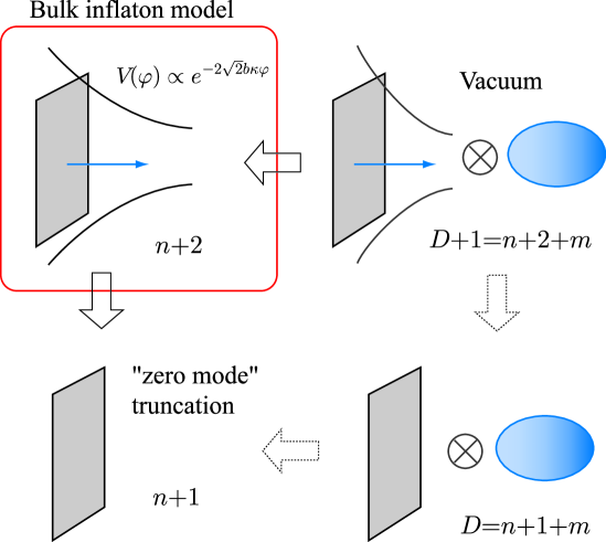
Figure 1: Schematic of the higher dimensional vacuum description of an $(n+2)$-dimensional bulk inflaton model and the derivation of the $(n+1)$-dimensional effective theory on the brane. The top-left picture represents the bulk inflaton model which we are interested in. To analyze cosmological background solutions (and “zero mode” perturbations), we use the $(n+1)$-dimensional description shown in the bottom-left corner. On the other hand, we make use of the $(D+1)$-dimensional description presented in the top-right corner to simplify the perturbation analysis.

III Single scalar field in the bulk

From now on, for simplicity, we focus on models with a single bulk scalar field. The $m$-dimensional space represented by $e^{2\phi}d\sigma^{2}$ is compactified either on a torus $(K=0)$, on a sphere $(K=1)$, or on a compact hyperboloid $(K=-1)$. Using a canonically normalized field $\varphi:=\kappa^{-1}_{n+2}\sqrt{m(m+n)/n}~{}\phi$, the $(n+2)$-dimensional reduced action is written as

$$S^{(n+2)}=\int d^{n+2}x\sqrt{-\tilde{\cal G}}\left\{\frac{1}{2\kappa^{2}_{n+2}}R[\tilde{\cal G}]-\frac{1}{2}\tilde{\cal G}^{ab}\partial_{a}\varphi\partial_{b}\varphi-V(\varphi)\right\}-\int d^{n+1}x\sqrt{-q}~{}U(\varphi),$$ (14)

where the potentials are

$$V(\varphi)=-\frac{(m+n)(m+n+1)}{2\kappa_{n+2}^{2}\ell^{2}}e^{-2\sqrt{2}b\kappa_{n+2}\varphi}-\frac{Km(m-1)}{2\kappa_{n+2}^{2}}e^{-\sqrt{2}\kappa_{n+2}\varphi/nb},$$ (15)

$$U(\varphi)=\tilde{\sigma}e^{-\sqrt{2}b\kappa_{n+2}\varphi},$$ (16)

with

$$b:=\sqrt{\frac{m}{2n(m+n)}}.$$ (17)

If we assume that the metric $ds^{2}_{(D+1)}$ is given in the form of (6), the action can further reduced to the $(n+1)$-dimensional effective one on the brane. We write the $D$-dimensional part of the metric in the form of

$$ds^{2}_{(D)}=g_{\hat{A}\hat{B}}dx^{\hat{A}}dx^{\hat{B}}=g_{\hat{a}\hat{b}}^{(n+1)}(x)dx^{\hat{a}}dx^{\hat{b}}+e^{2\alpha(t)}d\sigma^{2}.$$ (18)

Then, comparing the coefficient in front of $d\sigma^{2}$,

$$\phi(t,z):=\alpha(t)+\omega(z),$$ (19)

follows. Also, $(n+2)$-dimensional metric $\tilde{{\cal G}}_{ab}$ is written as

$$\tilde{\cal G}_{ab}dx^{a}dx^{b}=e^{2m\phi/n}{\cal G}_{ab}dx^{a}dx^{b}=e^{2(m+n)\omega/n}\left(q_{\hat{a}\hat{b}}dx^{\hat{a}}dx^{\hat{b}}+e^{2m\alpha/n}dz^{2}\right),$$ (20)

where we have set $e^{\omega(z_{b})}=1$. Substituting the above expression into (14), we perform the integration over $z$ to obtain

$$S^{(n+1)}=\frac{1}{2\kappa^{2}_{n+1}}\int d^{n+1}x\sqrt{-q}\Bigl{\{}e^{m\alpha/n}R[q] - \frac{m(m+n)}{n}e^{m\alpha/n}q^{\hat{a}\hat{b}}\partial_{\hat{a}}\alpha\partial_{\hat{b}}\alpha$$ (22)

$$-2\Lambda_{b}e^{-m\alpha/n}+Km(m-1)e^{-2\alpha-m\alpha/n}\Bigr{\}},$$

where

$$\kappa^{2}_{n+1}=\kappa^{2}_{D}/{\cal V},$$

with

$$\kappa^{2}_{D}:=\kappa^{2}_{D+1}\left[2\int^{\infty}_{z_{b}}e^{(m+n)\omega}dz\right]^{-1},$$

and ${\cal V}$ is the volume of the $m$-dimensional compactified space.

The above reduction to $(n+1)$ dimensions can be done more easily, starting with the $(D+1)[=n+2+m]$-dimensional action. First we perform the integration over $z$ and obtain a $D$-dimensional effective action,

$$S^{(D)}=\frac{1}{2\kappa_{D}^{2}}\int d^{D}x\sqrt{-g}(R[g]-2\Lambda_{b}),$$ (23)

where $\Lambda_{b}$ is, as before, the one defined by Eq. (5). The obtained effective action is that for $D$-dimensional pure gravity with a cosmological constant $\Lambda_{b}$. Compactifying $m$-dimensions further, and taking into account

$$q_{\hat{a}\hat{b}}=e^{2m\alpha/n}g_{\hat{a}\hat{b}}^{(n+1)},$$ (24)

the same expression for the $(n+1)$-dimensional effective action (22) can be recovered in a parallel way as we did for the reduction from $(D+1)$ dimensions to $(n+2)$ dimensions. Using $\varphi_{BD}:=e^{m\alpha/n}$ and $\omega_{BD}:=\sqrt{n(m+n)/m}$, we can rewrite the action into a familiar form:

$$S^{(n+1)}=\frac{1}{2\kappa^{2}_{n+1}}\int d^{n+1}x\sqrt{-q}\left\{\varphi_{BD}R-\frac{\omega_{BD}}{\varphi_{BD}}(\partial\varphi_{BD})^{2}-2\Lambda_{b}\varphi_{BD}^{-1}+Km(m-1)\varphi_{BD}^{-(m+2n)/m}\right\},$$ (25)

which implies that the effective theory on the brane is described by a scalar-tensor theory. The action (22), or equivalently (25), describes not only the background unperturbed cosmology but also the zero mode perturbation, both of which are independent of the extra-dimensional coordinate, $z$, apart from the overall factor $e^{2\omega}$.

The induced metric on the brane $q_{ab}$ is the metric in the Jordan frame. If we use the metric in the Einstein frame,

$$\tilde{q}_{\hat{a}\hat{b}}=e^{\frac{2m}{n(n-1)}\alpha}q_{\hat{a}\hat{b}},$$ (26)

the effective action becomes

$$S^{(n+1)}=\int d^{n+1}x\sqrt{-\tilde{q}}\left\{\frac{1}{2\kappa^{2}_{n+1}}R[\tilde{q}]-\frac{1}{2}\tilde{q}^{\hat{a}\hat{b}}\partial_{\hat{a}}\tilde{\varphi}\partial_{\hat{b}}\tilde{\varphi}-\tilde{V}(\tilde{\varphi})\right\},$$ (27)

where $\tilde{\varphi}:=\kappa_{n+1}^{-1}\sqrt{m(m+n)/n}~{}\alpha$ and the potential is

$$\kappa_{n+1}^{2}\tilde{V}(\tilde{\varphi})=\Lambda_{b}e^{-{2\sqrt{2}n\over n-1}b\kappa_{n+1}\tilde{\varphi}}-\frac{Km(m-1)}{2}e^{-{2\sqrt{2}n(m+n-1)\over m(n-1)}b\kappa_{n+1}\tilde{\varphi}}.$$ (28)

Obviously, the system defined by the above action is equivalent to Einstein gravity with a scalar field. A discussion on this type of potential can be found in a recent paper by Neupane Neupane:2003cs .

IV Examples of the background spacetime

In this section, we give some examples of $D$-dimensional vacuum solutions, which generate $(D+1)$-dimensional braneworld solutions by making use of the prescription described in Sec. II.1. Here we discuss models with a single scalar field and investigate their cosmological evolution in detail. Generalization to the case of multi scalar fields is given in Appendix B.

IV.1 Kasner type solutions

We first consider the following Kasner-type solution as an example of the Ricci-flat case, $\Lambda_{b}=0$,

$$g_{\hat{A}\hat{B}}dx^{\hat{A}}dx^{\hat{B}}=e^{2\alpha(\eta)}\left[-d\eta^{2}+\gamma_{\mu\nu}dy^{\mu}dy^{\nu}\right]+e^{2\beta(\eta)}\delta_{ij}dx^{i}dx^{j},$$

where $\gamma_{\mu\nu}$ is the metric of $m$-dimensional constant curvature space, and $i$ and $j$ run from 1 to $n$. Under the assumption of the above metric form, we solve the vacuum Einstein equations,

$$e^{2\alpha}R_{\eta}^{~{}\eta}=n\left[{\beta^{\prime}}^{2}-\alpha^{\prime}\beta^{\prime}+\beta^{\prime\prime}\right]+m\alpha^{\prime\prime}=0,$$ (29)

$$e^{2\alpha}R_{\mu}^{~{}\nu}=\delta_{\mu}^{~{}\nu}\left[K(m-1)+n\alpha^{\prime}\beta^{\prime}+(m-1){\alpha^{\prime}}^{2}+\alpha^{\prime\prime}\right]=0,$$ (30)

$$e^{2\alpha}R_{i}^{~{}j}=\delta_{i}{}^{j}\left[n{\beta^{\prime}}^{2}+(m-1)\alpha^{\prime}\beta^{\prime}+\beta^{\prime\prime}\right]=0,$$ (31)

where prime denotes differentiation with respect to $\eta$. Eliminating $\alpha^{\prime\prime}$ and $\alpha^{\prime}$ from the above three equations, we have

$$\beta^{\prime\prime}=\mp\sqrt{\frac{n(m+n-1)}{m}{\beta^{\prime}}^{4}-K(m-1)^{2}{\beta^{\prime}}^{2}}.$$

We can easily integrate this equation. For example, when $K=1$ (compactified on $m$-sphere $S^{m}$), the solution of this equation becomes

$$n\beta^{\prime}=\frac{\pm(m-1)q}{\sin[(m-1)\eta]},$$

where

$$q:=\sqrt{\frac{mn}{m+n-1}},$$ (32)

and the integration constant was used to shift the origin of time. Thus we find

$$e^{\beta}=\left[\tan\left(\frac{m-1}{2}\eta\right)\right]^{\pm q/n}.$$

Substituting this result into Eq. (31), we have

$$\alpha^{\prime}=\cot[(m-1)\eta]\mp\frac{q}{\sin[(m-1)\eta]}.$$

This is integrated as

$$e^{(m-1)\alpha}=\sin[(m-1)\eta]\left[\cot\left(\frac{m-1}{2}\eta\right)\right]^{\pm q}.$$

The solution for $K=-1$ is easily obtained by replacing $\sin$, $\tan$ and $\cot,$ in the above expressions by $\sinh,\tanh$ and $\coth$, respectively. The solution for $K=0$ behaves like $e^{\beta}\propto\eta^{\pm q/n}$ and $e^{(m-1)\alpha}\propto\eta^{1\mp q}$.

Let us further investigate the cosmology of the above example. Setting $n=3$ and $K=1$, the induced four-dimensional metric becomes

$$q_{\hat{a}\hat{b}}dx^{\hat{a}}dx^{\hat{b}}=e^{2m\alpha/3}\left[-e^{2\alpha}d\eta^{2}+e^{2\beta}\delta_{ij}dx^{i}dx^{j}\right],$$ (33)

where

$$e^{\alpha} = \left\{\sin[(m-1)\eta]\right\}^{\frac{1}{m-1}}\left\{\cot[(m-1)\eta/2]\right\}^{\frac{q}{m-1}},$$

$$e^{\beta} = \left\{\tan[(m-1)\eta/2]\right\}^{q/3},$$ (34)

and $q=\sqrt{3m/(m+2)}$ . We set $q$ to be positive without any loss of generality since the signature of $q$ is flipped by a shift of the origin of time, $\eta\to\eta+\pi$. Here one remark is in order. In the original $(D+1)$-dimensional model $m$ represents the number of the compactified dimensions and therefore is supposed to be an integer. However, $m$ is just a number parameterizing the form of the scalar field potential when we start with the action (14) obtained after dimensional reduction. We therefore find that $m$ can be any real positive number in this context. The positivity needs to be assumed to keep the appropriate signature of the kinetic term for the scalar field $\phi$, or equivalently to keep the relation between $\phi$ and $\varphi$ to be real. (Strictly speaking, the case with $m<-n=-3$ is also allowed.) Then, $q$ can be regarded as a continuous parameter with its range $0<q<\sqrt{3}$.

The cosmological time $\tau$ is related to $\eta$ via

$$d\tau=e^{(m+3)\alpha/3}d\eta.$$ (35)

Recall that $q_{\hat{a}\hat{b}}$, the metric induced on the brane in the five$[=n+2]$-dimensional model (14), is related to $g_{\hat{a}\hat{b}}$ by Eq. (24). Hence the scale factor associated with the metric $q_{\hat{a}\hat{b}}$ is given by $a=e^{m\alpha/3+\beta}$, and therefore the Hubble parameter on the brane $H:=a^{-1}da/d\tau$ is given by $H=(m\alpha^{\prime}/3+\beta^{\prime})e^{-m\alpha/3-\alpha}.$ Substituting the above solution (34) into these expressions, we obtain

$$a = \left\{\sin[(m-1)\eta]\right\}^{\frac{2q^{2}}{9(q^{2}-1)}}\left\{\tan[(m-1)\eta/2]\right\}^{\frac{q(q^{2}-3)}{9(q^{2}-1)}},$$

$$H = {q\left(q^{2}-3+2q\cos[(m-1)\eta]\right)\over 3(q^{2}-3)}\left\{\sin[(m-1)\eta]\right\}^{-\frac{8q^{2}}{9(q^{2}-1)}}\left\{\tan[(m-1)\eta/2]\right\}^{-\frac{q(q^{2}-9)}{9(q^{2}-1)}}.$$

The relation between the coordinate time $\eta$ and the cosmological time $\tau$ (35) is not so obvious, but the asymptotic behavior can be easily studied. When $\eta\to 0$, we have $\tau\propto\eta^{\frac{q(q+9)}{9(q+1)}}\to 0$ and

$$a \propto \eta^{\frac{q(q+3)}{9(q+1)}}\propto\tau^{p_{-}},$$

$$H \propto \eta^{-\frac{q(q+9)}{9(q+1)}}\propto a^{-\frac{q+9}{q+3}},$$

$$e^{\alpha} \propto \eta^{-\frac{3-q^{2}}{3(q+1)}}\to+\infty,$$

where the exponent $p_{-}$ is defined below in Eq. (36). For $\bar{\eta}:=\eta-\pi/(m-1)\to 0$, the cosmological time is (locally) expressed as $\tau\propto\bar{\eta}^{-\frac{q(q-9)}{9(q-1)}}$. Therefore the range of the proper time $\tau$ is infinite for the parameter region $0<q<1$, while it is finite for $1<q<\sqrt{3}$. In this limit $\bar{\eta}\to 0$, the scale factor, the Hubble parameter, and the scalar field behave like

$$a \propto \bar{\eta}^{-\frac{q(q-3)}{9(q-1)}}\propto\left\{{\tau^{p_{+}},~{}~{}~{}~{}~{}~{}~{}~{}~{}~{}(0<q<1),\atop(\tau_{end}-\tau)^{p_{+}},~{}~{}~{}(1<q<\sqrt{3}),}\right.$$

$$H \propto \bar{\eta}^{\frac{q(q-9)}{9(q-1)}}\propto a^{-\frac{q-9}{q-3}},$$

$$e^{\alpha} \propto \bar{\eta}^{-\frac{3-q^{2}}{3(1-q)}}\to\left\{{+\infty,~{}~{}~{}(0<q<1),\atop 0,~{}~{}~{}~{}(1<q<\sqrt{3}).}\right.$$

In the above expressions, we have used

$$p_{\pm}:=\frac{m+3}{4m+9\pm\sqrt{3m(m+2)}}.$$ (36)

The ranges of $p_{+}$ and $p_{-}$ are $1/(4+\sqrt{3})<p_{+}<1/3$ and $1/3<p_{-}<1/(4-\sqrt{3})$.

The behavior of this solution is easily understood from the viewpoint of the four-dimensional effective theory described by the action (27), as was discussed in Ref. Emparan:2003gg . The potential (28) with $\Lambda_{b}=0$ and $K=1$ is shown in FIG. 2. For $0<q<1$ ($0<m<1$) the potential is positive, while for $q>1$ $(m>1)$ the potential is negative. In the former case, the scalar field $\alpha$ starts at $\alpha=\infty$, climbs up the slope of the potential, turns around somewhere, and finally goes back to $\alpha=\infty$. In the latter case, $\alpha$ starts to roll down from $\alpha=\infty$. The universe expands for a period of time and eventually it starts to contract. Finally $\alpha$ falls into the bottomless pit within a finite time, where the universe ends up with a singularity.

Here we note that the above picture based on the four-dimensional effective theory describes the dynamics in the conformally transformed frame in which the metric is given by $\tilde{q}_{\hat{a}\hat{b}}$, whereas we suppose that the “physical” metric is given by the induced metric on the brane $q_{\hat{a}\hat{b}}$. In principle, the cosmic expansion law can look very different depending on the frame we choose. The dynamics in the “physical” frame therefore can be very different apparently. However, the above discussion is still useful since the conformal rescaling does not change the causal structure of the spacetime.

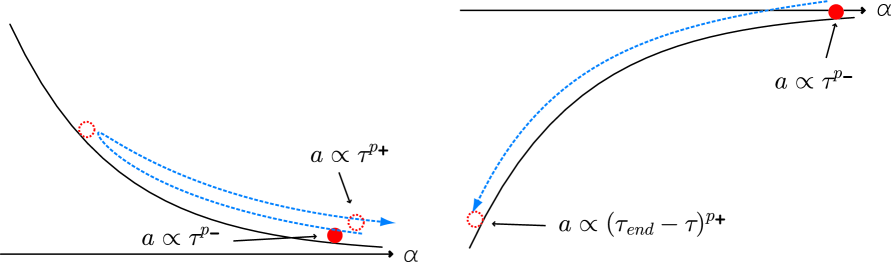
Figure 2: The motion of the scalar field in the potential. The behavior of the scale factor in the Jordan frame is also presented. The potential is positive for $0<q<1$ (left figure), whereas it is negative for $1<q<\sqrt{3}$ (right figure).

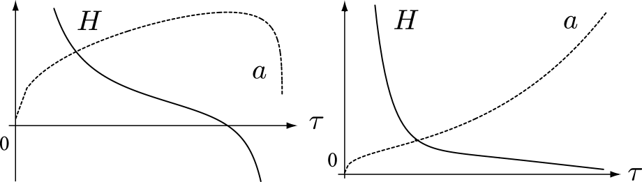
Figure 3: The sketch of the behavior of the scale factor $a$ (dashed lines) and the Hubble parameter $H$ (solid lines) in the Jordan frame as functions of the proper time on the brane $\tau$. The left figure shows the solution of (34) with $q>1$. The right figure describes the solution of (41) with the plus sign in the exponent.

IV.2 Kasner type solutions with a cosmological constant

The next example is a generalization of the Kasner-type spacetime including a cosmological constant $\Lambda_{b}$. Let us assume that the metric is in the form of

$$g_{\hat{A}\hat{B}}dx^{\hat{A}}dx^{\hat{B}}=-dt^{2}+e^{2\alpha(t)}\delta_{\mu\nu}dy^{\mu}dy^{\nu}+e^{2\beta(t)}\delta_{ij}dx^{i}dx^{j},$$ (37)

where $i$ and $j$ again run from 1 to $n$, but here the metric of $m$-dimensional space is chosen to be flat ($K=0$) because otherwise the solution with $\Lambda_{b}\neq 0$ is not obtained analytically. The $D[=n+1+m]$-dimensional vacuum Einstein equations with a cosmological constant reduce to

$$m\left(\ddot{\alpha}+\dot{\alpha}^{2}\right)+n\left(\ddot{\beta}+\dot{\beta}^{2}\right)=(m+n)H_{0}^{2},$$ (38)

$$\ddot{\alpha}+\dot{\alpha}\left(m\dot{\alpha}+n\dot{\beta}\right)=(m+n)H_{0}^{2},$$ (39)

$$\ddot{\beta}+\dot{\beta}\left(m\dot{\alpha}+n\dot{\beta}\right)=(m+n)H_{0}^{2}.$$ (40)

From this we obtain two types of solutions (see Appendix B). One is a trivial solution, namely, $D$-dimensional de Sitter spacetime,

$$\alpha=\beta=H_{0}t.$$

Of the other type is the following two solutions,

$$e^{m\alpha+n\beta}=\sinh[(m+n)H_{0}t],$$

$$e^{\alpha-\beta}=\left[\tanh\left(\frac{m+n}{2}H_{0}t\right)\right]^{\pm 1/q},$$ (41)

where $q$ is the one that has been introduced in Eq. (32). The range of the time coordinate $t$ is $(-\infty,\infty)$ for the former de Sitter solution and $[0,\infty)$ for the latter non-trivial solutions. Applying the method discussed in Sec. II.1 to these solutions, one can construct background solutions for a $(D+1)$-dimensional braneworld model.

First we briefly mention the relation to the bulk inflaton model recently proposed by Koyama and Takahashi Koyama:2003yz ; Koyama:2003sb . Identifying their model parameters $\Delta$ and $\delta$ as

$$\Delta=4b^{2}-8/3=-\frac{2(m+4)}{m+3},\qquad\delta=\frac{m+4}{4(m+3)}\frac{\ell^{2}H_{0}^{2}}{1+\ell^{2}H_{0}^{2}},$$ (42)

we will find that our model is equivalent to theirs. The parameter $m$ is supposed to take any positive number. Thus it follows that $\Delta$ varies in the same region, $-8/3\leq\Delta\leq-2$, considered in Koyama:2003yz ; Koyama:2003sb . The background metric obtained by substituting the simplest solution $\alpha=\beta=H_{0}t$ is indeed the case discussed in their paper.

Next we consider the cosmic expansion law. We start with the simplest case $\alpha=\beta=H_{0}t$. The dimensionally reduced metric (on the brane) is

$$q_{\hat{a}\hat{b}}dx^{\hat{a}}dx^{\hat{b}}=e^{2mH_{0}t/3}\left(-dt^{2}+e^{2H_{0}t}\delta_{ij}dx^{i}dx^{j}\right).$$

Introducing the cosmological time $\tau$ and the conformal time $\eta$ defined by

$$d\tau=ad\eta=e^{mH_{0}t/3}dt,$$

the scale factor on the brane $a=e^{(m+3)H_{0}t/3}$ is written in terms of $\tau$ or $\eta$ as

$$a\propto\tau^{(m+3)/m}\propto\eta^{-(m+3)/3}.$$ (43)

Since $1\leq(m+3)/m<\infty$, power-law inflation with any exponent can be realized.

Furthermore, we have non-trivial solutions (41). The behavior of the solutions is as follows. At early times ($t\sim 0$), the scale factor behaves like $a=e^{m\alpha/3+\beta}\sim t^{1/3}$, and the cosmological time is given by $d\tau\sim t^{\left(m\pm\sqrt{3m(m+2)}\right)/3(m+3)}dt$ (and so $\tau\to 0$ as $t\to 0$). Therefore, we have

$$a\sim\tau^{p_{\pm}},$$ (44)

with $p_{\pm}$ introduced previously, which implies that the universe is not accelerated at early times. At late times ($t\to\infty$), we see that $\alpha\to H_{0}t$ and $\beta\to H_{0}t$, and the solution shows power-law expansion as is given in Eq. (43).

A rather intuitive interpretation of the behavior of these three solutions can be made from the four-dimensional point of view again. The situation is summarized in FIG. 4. This time the potential is always positive. For one of the non-trivial solutions with the exponent $p_{+}$ in (44), the scalar field starts to roll down from $\alpha=-\infty$. For the other non-trivial solution with the exponent $p_{-}$, the field starts to climb up the slope of the potential from $\alpha=+\infty$, turns around somewhere, and rolls down back to $\alpha=+\infty$. Suppose that the field $\alpha$ is increasing. Let us trace the evolution of $\alpha$ backward in time. If the kinetic energy is larger than a certain critical value, $\alpha$ will not have a turning point in the past. In this case $\alpha$ continues to decrease, reaching $-\infty$. This corresponds to the case with the exponent $p_{+}$. If the kinetic energy is lower, $\alpha$ will have a turning point. Then, we will have $\alpha\to+\infty$ at $t\to-\infty$. This corresponds to the case with the exponent $p_{-}$. The case of the power-law inflation (43) is, in fact, the marginal case between these two. In this case, $\alpha$ does not turn around. Therefore the evolution of $\alpha$ is similar to the case with $p_{+}$. In any case, information about the initial velocity is lost as the universe expand. Therefore the late time behavior of the solutions is unique, and is given by Eq. (43).

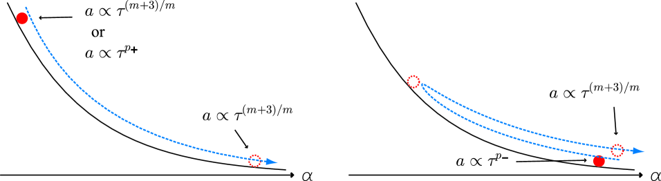
Figure 4: The motion of the scalar field in the potential and the behavior of the scale factor in the Jordan frame. The solution found by Koyama and Takahashi Koyama:2003yz ; Koyama:2003sb is described in the left figure. One of the non-trivial solutions with its behavior at the starting point $a\propto\tau^{p_{+}}$ is also shown in the left figure, while the other one with the exponent $p_{-}$ behaves as shown in the right figure.

V Cosmological perturbations

We consider cosmological perturbations in the $(n+2)$-dimensional bulk inflaton models defined by (12) and (13). The analysis of perturbations is complicated if we work in the original $(n+2)$-dimensional models with a bulk scalar field. Our $(n+2)$-dimensional system, however, is equivalent to the $(D+1)[=n+2+m]$-dimensional one defined by (2) and (3). We will show that the perturbation analysis becomes very simple and transparent in the $(D+1)$-dimensional picture, in which we just need to consider pure gravity without any matter fields.

We begin with the following form of background metric:

$$G_{AB}dX^{A}dX^{B}=e^{2\omega(z)}\left(dz^{2}-dt^{2}+e^{2\alpha(t)}\gamma_{\mu\nu}dy^{\mu}dy^{\nu}+e^{2\beta(t)}\delta_{ij}dx^{i}dx^{j}\right),$$ (45)

where latin and roman indices in the lower case, respectively, rum $m$ and $n$-dimensional subspaces, and the warp factor is given by $e^{\omega(z)}=\ell H_{0}/\sinh(H_{0}z)$. We assume that $\alpha(t)$ and $\beta(t)$ are chosen so that $g_{\hat{A}\hat{B}}$ be a solution of the $(n+1+m)$-dimensional vacuum Einstein equations with a cosmological constant,

$$m\left(\ddot{\alpha}+\dot{\alpha}^{2}\right)+n\left(\ddot{\beta}+\dot{\beta}^{2}\right)=(m+n)H_{0}^{2},$$ (46)

$$\ddot{\alpha}+\dot{\alpha}\left(m\dot{\alpha}+n\dot{\beta}\right)+K(m-1)e^{-2\alpha}=(m+n)H_{0}^{2},$$ (47)

$$\ddot{\beta}+\dot{\beta}\left(m\dot{\alpha}+n\dot{\beta}\right)=(m+n)H_{0}^{2}.$$ (48)

The background solutions with $\gamma_{\mu\nu}=\delta_{\mu\nu}~{}(K=0),~{}H_{0}\neq 0$ and with $K=\pm 1,~{}H_{0}=0$ were discussed in the preceding section. In the following discussions, we include more general cases with $K=\pm 1$ and $H_{0}\neq 0$. Although the background solution cannot be obtained in an explicit form for such non-flat compactifications with a cosmological constant, we will find that general properties of perturbations can be explored to a great extent.

We write the perturbed metric as

$$(G_{AB}+\delta G_{AB})dX^{A}dX^{B}$$

$$\qquad=e^{2\omega}\big{\{}(1+2N)dz^{2}+2Adtdz-(1+2\Phi)dt^{2}+e^{2\alpha}(1+2S)\gamma_{\mu\nu}dy^{\mu}dy^{\nu}$$

$$\qquad\qquad+e^{2\beta}\left[(1+2\Psi)\delta_{ij}dx^{i}dx^{j}+2E_{ij}dx^{i}dx^{j}+2B_{i}dx^{i}dt+2C_{i}dx^{i}dz\right]\big{\}}.$$ (49)

These perturbations are assumed to be homogeneous and isotropic in the directions of the $m$-dimensional compactified space spanned by the coordinates $y^{\mu}$. From the assumption of isotropy, mixed components such as $\delta G_{\mu t}dy^{\mu}dt$ and $\delta G_{\mu i}dy^{\mu}dx^{i}$ are set to zero. Concerning the metric perturbations of the compactified space, therefore only the overall volume perturbation $S$ is considered. After reduction to $(n+2)$-dimensions, $S$ is to be interpreted as the scalar field perturbation. Here, we also assume that the dependence on the $n$-dimensional coordinates $x^{i}$ is given by $e^{ik_{i}x^{i}}$.

Metric perturbations are decomposed into scalar, vector, and tensor components based on the behavior under the transformation of the $n$-dimensional spatial coordinates $x^{i}$ in the following manner:

$$B_{i}=\frac{k_{i}}{ik}B^{S}+B^{V}_{i},~{}~{}k^{i}B^{V}_{i}=0,$$

$$E_{ij}=\left(-\frac{k_{i}k_{j}}{k^{2}}+\frac{\delta_{ij}}{n}\right)E^{S}+\frac{1}{ik}k_{(i}E_{j)}^{V}+\frac{1}{2}E_{ij}^{T},$$

$$k^{i}E_{i}^{V}=k^{i}E_{ij}^{T}=0,~{}~{}\delta^{ij}E^{T}_{ij}=0.$$ (50)

The quantities with a superscript $S$, $V$ and $T$ represent scalar, vector and tensor perturbations, respectively. The perturbations $\delta G_{AB}$ obey the linearized Einstein equations supplemented by boundary conditions at the position of the brane, $\delta{\cal K}_{A}^{~{}B}|_{z=z_{b}}=0$ where ${\cal K}_{AB}$ is the extrinsic curvature of the brane. From the $(D+1)$-dimensional point of view matter sources are absent on the $D$-dimensional brane, and this makes boundary conditions considerably simple. Each component of the Einstein equations is presented in Appendix A.

Here we would like to discuss the number of physical degrees of freedom in scalar, vector, and tensor perturbations. The transverse traceless tensor $E_{ij}^{T}$ has $(n+1)(n-2)/2$ independent components, each of which obeys a second order differential equation. For vector perturbations there are three variables $B_{i}^{V}$, $E_{j}^{V}$ and $C_{i}^{V}$. The coordinate transformation has one vector mode, and correspondingly there is one vector constraint equation. Therefore we have only $1[=3-1\times 2]$ vector remaining as a physical mode. Since a transverse vector has $(n-1)$ independent components, we find that there are $1\times(n-1)$ degrees of freedom in vector perturbations, corresponding to the “graviphoton”. For scalar perturbations there are 8 variables, and the coordinate transformation has 3 independent modes. Since there are the same number of constraint equations, the number of physical modes is $2[=8-3\times 2]$. One of them corresponds to the bulk scalar field and the other corresponds to the “graviscalar”. In total, there are $1+(n+2)(n-1)/2=2+(n-1)+(n+1)(n-2)/2$ physical degrees of freedom. The first “1” on the left hand side corresponds to the bulk scalar and the other $(n+2)(n-1)/2$ degrees of freedom to those of $(n+2)$-dimensional gravitational waves.

V.1 Tensor perturbations

Since tensor perturbations are gauge-invariant from the beginning, they are in general easy to analyze. The equations for tensor perturbations are read from the $\{i,j\}$-component of the Einstein equations (120) as

$${\cal L}E^{T}_{ij}=0,$$ (51)

where we have defined a differential operator

$${\cal L}:=\partial^{2}_{t}+\left(m\dot{\alpha}+n\dot{\beta}\right)\partial_{t}+e^{-2\beta}k^{2}-\partial_{z}^{2}-(m+n)(\partial_{z}\omega)\partial_{z}.$$

The perturbed junction condition implies that boundary conditions are Neumann on the brane,

$$\left.\partial_{z}E^{T}_{ij}\right|_{z=z_{b}}=0.$$ (52)

Since the perturbation equations are manifestly separable, we write $E^{T}_{ij}=\chi(t)\psi(z)Y^{T}_{ij}(x^{\ell})$ where $Y^{T}_{ij}$ is a transverse, traceless tensor harmonics. Then $\chi(t)$ and $\psi(z)$ obey

$$\ddot{\chi}+\left(m\dot{\alpha}+n\dot{\beta}\right)\dot{\chi}+\left(e^{-2\beta}k^{2}+M^{2}\right)\chi=0,$$ (53)

$$\quad\partial_{z}^{2}\psi+(m+n)(\partial_{z}\omega)\partial_{z}\psi+M^{2}\psi=0.$$ (54)

Here $M^{2}$ is a separation constant and represents the squared Kaluza-Klein mass for observers on the $D$-dimensional brane.

Now we discuss the mode function in the $z$-direction $\psi(z)$. Using a canonical variable $\hat{\psi}:=e^{\mu\omega}\psi$, with

$$\mu:=\frac{m+n}{2}\geq\frac{3}{2},$$ (55)

Eq. (54) is rewritten into a Schrödinger-type equation,

$$-\partial_{z}^{2}\hat{\psi}+V(z)\hat{\psi}=M^{2}\hat{\psi},$$ (56)

where the potential is

$$V(z)=\mu(\mu+1)\frac{H_{0}^{2}}{\sinh^{2}(H_{0}z)}+\mu^{2}H_{0}^{2}-\frac{\kappa_{D+1}^{2}\sigma}{2}\delta(z-z_{b}).$$ (57)

The delta-function term is introduced so that $\psi$ automatically satisfies the boundary condition $\psi^{\prime}(z_{b})=0$. The presence of the zero mode, for which $\psi$ is constant in $z$, is obvious from Eq. (54). From the asymptotic value of the potential $V(\infty)=\mu^{2}H_{0}^{2}$, we can say that there is a mass gap $\delta M=\mu H_{0}$ between the zero mode and the KK continuum.

The $z$-dependence of the massive modes are given in terms of the associated Legendre functions by

$$\psi_{M}(z)= c^{T}(\sinh(H_{0}z))^{1/2+\mu} \Biggl{[}Q_{1/2+i\nu}^{-1/2-\mu}(\cosh(H_{0}z_{b}))P_{-1/2+i\nu}^{-1/2-\mu}(\cosh(H_{0}z))$$ (59)

$$\qquad-P_{1/2+i\nu}^{-1/2-\mu}(\cosh(H_{0}z_{b}))Q_{-1/2+i\nu}^{-1/2-\mu}(\cosh(H_{0}z))\Biggr{]},$$

where $c^{T}$ is a normalization constant and

$$\nu:=\sqrt{\frac{M^{2}}{H_{0}^{2}}-\mu^{2}}.$$ (60)

These general properties of the mass spectrum and the mode functions in the $z$-direction hold irrespective of the specific form of the background solution $\alpha$ and $\beta$.

Let us move on to the time dependence of tensor perturbations. Using the cosmological time on the brane defined by $\tau=\int e^{m\alpha/n}dt$, Eq. (53) is rewritten as

$$\left[\frac{d^{2}}{d\tau^{2}}+\left(nH+\frac{m}{n}\frac{d\alpha}{d\tau}\right)\frac{d}{d\tau}+\frac{k^{2}}{a^{2}}+e^{-2m\alpha/n}M^{2}\right]\chi=0,$$ (61)

where one must recall that $a=e^{m\alpha/n+\beta}$ and $H=a^{-1}da/d\tau$. For the zero mode ($M^{2}=0$), this reduces to the equation for the tensor perturbations in the scalar-tensor theory defined by the action (22). An apparent difference from Einstein gravity is the presence of the term $(m/n)(d\alpha/d\tau)$. The Kaluza-Klein mass with respect to observers on the brane is expressed as

$$m^{2}_{{\rm KK}}(t)=e^{-2m\alpha(t)/n}M^{2},$$ (62)

and so $m_{{\rm KK}}=e^{-m\alpha/n}\mu H_{0}$ for the lightest one, whereas the Hubble parameter at that time is given by

$$H=e^{-m\alpha/n}\left(\frac{m}{n}\dot{\alpha}+\dot{\beta}\right).$$

For $\alpha=\beta=H_{0}t$, this implies $H=2n^{-1}e^{-m\alpha/n}\mu H_{0}$ and therefore the mass gap and $H$ are of the same order. On the other hand, when the background is given by Eq. (41), we have $H=2n^{-1}e^{-m\alpha/n}\mu H_{0}\coth[(m+n)H_{0}t]$ and the mass gap can be very small compared to $H$, but only for a short period near $t=0$.

Despite its rather simple form, Eq. (53) cannot be solved analytically in general. One exception is the case $\alpha=\beta=H_{0}t$ discussed in Koyama:2003yz . In this case, Eq. (53) reads

$$\ddot{\chi}+(m+n)H_{0}\dot{\chi}+\left(e^{-2H_{0}t}k^{2}+M^{2}\right)\chi=0,$$

which, using the conformal time $\eta=-e^{-H_{0}t}/H_{0}$, can be rewritten as

$$\left[\frac{d^{2}}{d\eta^{2}}+\frac{1-m-n}{\eta}\frac{d}{d\eta}+k^{2}+\frac{M^{2}}{H_{0}^{2}\eta^{2}}\right]\chi=0.$$ (63)

This indeed has analytic solutions,

$$\chi_{0}\propto(-\eta)^{\mu}H^{(1)}_{\mu}(-k\eta),$$ (64)

$$\chi_{M}\propto(-\eta)^{\mu}H^{(1)}_{i\nu}(-k\eta).$$ (65)

This is not a surprise because the background of the current model is just an AdS_m+2+n bulk with a de Sitter brane.

V.2 Vector perturbations

Next we consider vector perturbations. From perturbed junction conditions $\delta{\cal K}_{i}^{~{}j}|_{z=z_{b}}=0$ and $\delta{\cal K}_{i}^{~{}t}|_{z=z_{b}}=0$, we have

$$\left.\partial_{z}E_{i}^{V}\right|_{z=z_{b}}=0,~{}~{}\left.{C_{i}^{V}}\right|_{z=z_{b}}=0,~{}~{}\left.\partial_{z}B_{i}^{V}\right|_{z=z_{b}}=0.$$ (66)

Under a vector gauge transformation $x^{i}\to\bar{x}^{i}=x^{i}+\xi^{iV}$, metric variables transform as

$$\bar{E}_{i}^{V}=E^{V}_{i}+k\xi_{i}^{V},\qquad\bar{B}_{i}^{V}=B^{V}_{i}-\dot{\xi}_{i}^{V},\qquad\bar{C}_{i}^{V}=C^{V}_{i}-\partial_{z}{\xi_{i}^{V}}.$$ (67)

Thus we are allowed to set $E_{i}^{V}=0$ by choosing an appropriate gauge. We expand the remaining variables by using the transverse vector harmonics $Y^{V}_{i}$ as

$$B^{V}_{i}={\cal B}Y^{V}_{i},\qquad C^{V}_{i}={\cal C}Y^{V}_{i}.$$ (68)

For convenience, we introduce

$$\Omega:=k^{-2}e^{m\alpha+(n+2)\beta}e^{(m+n)\omega}\left(\partial_{z}{\cal B}-\dot{\cal C}\right).$$ (69)

Then Eqs. (123), and (126) are written as

$${\cal B}=e^{-m\alpha-n\beta}e^{-(m+n)\omega}\partial_{z}\Omega,$$ (70)

$${\cal C}=e^{-m\alpha+n\beta}e^{-(m+n)\omega}\dot{\Omega}.$$ (71)

It is easy to see that the remaining third equation is automatically satisfied if the above two equations hold. Substituting these two into Eq. (69), we obtain a master equation

$$\left[\ddot{\Omega}-\left(m\dot{\alpha}+n\dot{\beta}\right)\dot{\Omega}+e^{-2\beta}k^{2}\Omega\right]-\left[\partial_{z}^{2}\Omega-(m+n)(\partial_{z}\omega)\partial_{z}\Omega\right]=0.$$ (72)

This equation looks similar to the equation for tensor perturbations (51). The difference is that the signatures of the terms containing first-derivatives such as $\dot{\Omega}$ and $\Omega^{\prime}$ are reversed. From Eqs. (66), the boundary condition for $\Omega$ on the brane turns out to be Dirichlet,

$$\Omega|_{z=z_{b}}=0.$$ (73)

Since the master equation (72) is separable, we write $\Omega(t,z)=\chi(t)\Omega(z)$. The canonical variable, $\hat{\Omega}(z):=e^{-\mu\omega}\Omega$, again obeys a Schrödinger-type equation,

$$-\partial_{z}^{2}{\hat{\Omega}}+V(z)\hat{\Omega}=M^{2}\hat{\Omega},$$ (74)

with the potential

$$V(z)=\mu(\mu-1)\frac{H_{0}^{2}}{\sinh^{2}(H_{0}z)}+\mu^{2}H_{0}^{2}.$$ (75)

The crucial difference from tensor perturbations is the absence of the delta-function potential well. Because of this, there is no zero mode and only the massive modes with $M^{2}\geq V(\infty)=\mu^{2}H_{0}^{2}$ exist. The $z$-dependence of the mode functions are given by

$$\Omega_{M}(z)= c^{V}(\sinh(H_{0}z))^{1/2-\mu} \Biggl{[}Q_{-1/2+i\nu}^{-1/2+\mu}(\cosh(H_{0}z_{b}))P_{-1/2+i\nu}^{-1/2+\mu}(\cosh(H_{0}z))$$ (77)

$$\qquad-P_{-1/2+i\nu}^{-1/2+\mu}(\cosh(H_{0}z_{b}))Q_{-1/2+i\nu}^{-1/2+\mu}(\cosh(H_{0}z))\Biggr{]},$$

where $c^{V}$ is a normalization constant. When $\alpha=\beta=H_{0}t$, we can find an analytic solution for the time-dependence of the mode functions, which, using the conformal time, is given by

$$\chi_{M}(\eta)\propto(-\eta)^{-\mu}H^{(1)}_{i\nu}(-k\eta).$$

V.3 Scalar perturbations

V.3.1 Gauge choice, the boundary condition, and the mode decomposition

Since scalar perturbations are more complicated, we begin with fixing the gauge appropriately in order to simplify the perturbed Einstein equations. We impose the Gaussian-normal gauge conditions

$$N=A=C=0.$$ (78)

Different from the case of vector perturbations, these conditions do not fix the gauge completely. In the case of scalar perturbations we need to take care of perturbations of the brane location. Here we make use of the remaining gauge degrees of freedom to keep the brane location unperturbed at $z=z_{b}$. In the Gaussian-normal gauge, boundary conditions on the brane for all remaining variables become Neumann:

$$\partial_{z}\Psi|_{z=z_{b}}=\partial_{z}E|_{z=z_{b}}=\partial_{z}S|_{z=z_{b}}=\partial_{z}\Phi|_{z=z_{b}}=\partial_{z}B|_{z=z_{b}}=0.$$ (79)

Three of eight scalar perturbation equations are the constraint equations, and the other five are the evolution equations. First, let us examine the constraint equations (122), (128), and (129). Eq. (128) reduces to $\partial^{2}_{z}(\Phi+n\Psi+mS)+\partial_{z}\omega\partial_{z}(\Phi+n\Psi+mS)=0$. Taking into account the boundary conditions, this equation is once integrated to give

$$\partial_{z}(\Phi+n\Psi+mS)=0.$$ (80)

Eqs. (122) and (129) reduce to

$$\partial_{z}\left[kB+2\dot{\Phi}+2\left(m\dot{\alpha}+n\dot{\beta}\right)\Phi-2m\dot{\alpha}S-2n\dot{\beta}\Psi\right]=0,$$ (81)

$$\partial_{z}\left\{\dot{B}+\left(m\dot{\alpha}+n\dot{\beta}+2\dot{\beta}\right)B+2e^{-2\beta}k\left[\Psi+\left(\frac{1}{n}-1\right)E\right]\right\}=0.$$ (82)

With the aid of Eq. (80), we find that all the perturbation equations are separable. Furthermore, the $z$-dependent parts of these equations are the same as those of tensor perturbations with the same type of boundary conditions. Therefore we can expand all variables by using the same mode functions in the $z$-direction as those for tensor perturbations:

$$E=E_{0}(t)\psi_{0}(z)+\sum E_{M}(t)\psi_{M}(z),\qquad\Phi=\Phi_{0}(t)\psi_{0}(z)+\sum\Phi_{M}(t)\psi_{M}(z),\qquad\cdots,$$ (83)

where $\psi_{0}$ is constant, $\psi_{M}$ is given by Eq. (59), and $M^{2}\geq\mu^{2}H_{0}^{2}$. Consequently, Eqs. (80), (81), and (82) are automatically satisfied for the zero mode. For the massive modes these constraint equations give

$$\Phi+n\Psi+mS=0,$$ (84)

$$kB+2\dot{\Phi}+2\left(m\dot{\alpha}+n\dot{\beta}\right)\Phi-2m\dot{\alpha}S-2n\dot{\beta}\Psi=0,$$ (85)

$$\dot{B}+\left(m\dot{\alpha}+n\dot{\beta}+2\dot{\beta}\right)B+2e^{-2\beta}k\left[\Psi+\left(\frac{1}{n}-1\right)E\right]=0,$$ (86)

where the subscript $M$ was abbreviated. Note that these three equations are nothing but components of the divergence of the metric perturbations,

$$\nabla^{A}\delta G_{zA}=\nabla^{A}\delta G_{tA}=\nabla^{A}\delta G_{iA}=0.$$

In other words, the transverse traceless conditions are automatically satisfied if one impose the Gaussian normal gauge conditions except for the contribution coming from the zero mode. ($\nabla^{A}\delta G_{zA}$ gives the traceless condition.) Below we discuss the KK modes and the zero mode separately.

V.3.2 KK modes

By using the constraint equations (84)-(86), the Einstein equations (117), (118), (125), (127), and (130) are simplified to give

$${\cal L}\Psi=-\left(\frac{2}{n}-1\right)k\dot{\beta}B+2\dot{\beta}\dot{\Phi}+2(m+n)H_{0}^{2}\Phi,$$ (87)

$${\cal L}E=2k\dot{\beta}B,$$ (88)

$${\cal L}S=k\dot{\alpha}B+2\dot{\alpha}\dot{\Phi}+2e^{-2\alpha}K(m-1)(S-\Phi)+2(m+n)H_{0}^{2}\Phi,$$ (89)

$${\cal L}\Phi=-2\left(m\ddot{\alpha}+n\ddot{\beta}\right)\Phi+2k\dot{\beta}B+2m\ddot{\alpha}S+2n\ddot{\beta}\Psi+2(m+n)H_{0}^{2}\Phi,$$ (90)

$${\cal L}B=-\left(m\ddot{\alpha}+n\ddot{\beta}\right)B-4\dot{\beta}\dot{B}-4\dot{\beta}^{2}B-2(m+n)H_{0}^{2}B-4e^{-2\beta}k\dot{\beta}\Phi.$$ (91)

where ${\cal L}$ is defined in Eq. (V.1). Two of them give independent master equations for the massive modes, and the remaining three equations do not give any new conditions. With the aid of the constraint equations (84)-(86), Eqs. (87) and (90) can be rewritten as

$${\cal L}\Psi = -2(n-2)\dot{\beta}\left(\dot{\alpha}-\dot{\beta}\right)\Psi+{4\over n}\dot{\beta}\dot{\Phi}$$ (93)

$$\quad-2\left\{\frac{n-2}{n}\dot{\beta}\left[(m+1)\dot{\alpha}+n\dot{\beta}\right]-(m+n)H^{2}\right\}\Phi,$$

$${\cal L}\Phi = -4\dot{\beta}\dot{\Phi}-2\left\{(m+1)\ddot{\alpha}+n\ddot{\beta}+2\dot{\beta}\left[(m+1)\dot{\alpha}+n\dot{\beta}\right]-(m+n)H^{2}\right\}\Phi$$ (95)

$$\quad-2n\left[\ddot{\alpha}-\ddot{\beta}+2\dot{\beta}\left(\dot{\alpha}-\dot{\beta}\right)\right]\Psi.$$

Unfortunately, except for the simplest case (to be discussed later) we do not know how to disentangle these two equations, although there is no problem in solving these equations numerically. Once we could solve these coupled equations, the other variables $S,B,E$ are easily determined just by using the constraint equations.

V.3.3 Zero mode

To discuss the zero mode, it is useful to look at the cosmological perturbations in the corresponding $(n+1)$-dimensional theory defined by the action (27). In the case of the $(n+1)$-dimensional Friedmann universe with a single scalar field, there is only one physical degree of freedom in scalar perturbations. One can derive a second order differential equation for one master variable Mukhanov:1990me . Back in the braneworld context, the background metric and its zero-mode perturbations are also described by the same effective action (27). Therefore, the analysis of the zero mode is no different from the conventional $(n+1)$-dimensional cosmological perturbation theory. Below we will explain this fact more explicitly.

To begin with, we consider $(n+1+m)$-dimensional spacetime whose metric is given by

$$ds^{2}=-(1+2\Phi)dt^{2}+e^{2\alpha}(1+2S)\gamma_{\mu\nu}dy^{\mu}dy^{\nu}+e^{2\beta}\left[(1+2\Psi)\delta_{ij}dx^{i}dx^{j}+2E_{ij}dx^{i}dx^{j}+2B_{i}dx^{i}dt\right],$$ (96)

where only scalar perturbations are imposed and they are again assumed to be homogeneous and isotropic with respect to the $m$-dimensional compactified space spanned by $y^{\mu}$. Then, the perturbed Einstein equations $\delta R_{\hat{A}\hat{B}}=(m+n)H_{0}^{2}\delta g_{\hat{A}\hat{B}}$ become identical to Eqs. (117), (118), (125), (127), and (130) with $N$, $A$, $C$, and the terms differentiated by $z$ dropped. Hence, it is manifest that the analysis of zero-mode perturbations in our $(n+2+m)$-dimensional spacetime is equivalent to that of the above system.

As for perturbations in $(n+2+m)$-dimensional spacetime, we have already fixed the gauge by imposing three gauge conditions (78). However, these gauge conditions do not fix the gauge completely. As is manifest from Eqs. (132), gauge transformations satisfying $\xi^{z}=0$ and ${\xi^{S}}^{\prime}={\xi^{t}}^{\prime}=0$ do not disturb the conditions (78). On the other hand, on the $(n+1)$-dimensional side there are two scalar gauge transformations

$$t\to\bar{t}=t+\xi^{t}$$

$$x^{i}\to\bar{x}^{i}=x^{i}+k^{i}\xi^{S}/ik.$$

The transformation of metric variables under these gauge transformations is the same as that obtained by setting $\xi^{z}=0$ and ${\xi^{S}}^{\prime}={\xi^{t}}^{\prime}=0$ in the last five equations in (132).

If we think of the size of compactified dimension $S$ as a scalar field in $(n+1)$-dimensional spacetime, the system reduces to a conventional $(n+1)$-dimensional model with a scalar field. In the conventional cosmological perturbation theory, $\Phi$ and $\Psi$ in the longitudinal gauge $(B=E=0)$ are known to be convenient variables. Here one remark is that we need to take account of a conformal transformation to map the theory to the conventional $(n+1)$-dimensional one,

$$d\tilde{s}^{2}=e^{\frac{2m}{n(n-1)}(\alpha+S)}\cdot e^{\frac{2m}{n}(\alpha+S)}ds^{2}=e^{\frac{2m}{n-1}(\alpha+S)}ds^{2},$$ (97)

which follows from the discussion in Sec. III. Then, the variables corresponding to the so-called Sasaki-Mukhanov variables are

$$\hat{\Phi}:=\Phi+\frac{m}{n-1}S,$$ (98)

$$\hat{\Psi}:=\Psi+\frac{m}{n-1}S,$$ (99)

in the longitudinal gauge.

Eliminating $N$, $A$, $B$, $C$, $E$ and the terms differentiated by $z$, Eq. (118) becomes

$$\hat{\Phi}+(n-2)\hat{\Psi}=0.$$ (100)

Similarly, from Eqs. (125), (117) and (130), we have

$$(n-1)\dot{\hat{\Psi}}+(n-2)\left[m\dot{\alpha}+(n-1)\dot{\beta}\right]\hat{\Psi}=-\frac{m+n-1}{n-1}m\dot{\alpha}S.$$ (101)

$${\cal L}_{0}\Psi=-2(n-1)\dot{\beta}\dot{\hat{\Psi}}+2(m+n)H_{0}^{2}\Phi,$$ (102)

$${\cal L}_{0}S=-2\dot{(}n-1)\alpha\dot{\hat{\Psi}}+2(m+n)H_{0}^{2}\Phi-2K(m-1)e^{-2\alpha}(\Phi-S),$$ (103)

where ${\cal L}_{0}f:=\ddot{f}+\left(m\dot{\alpha}+n\dot{\beta}\right)\dot{f}+e^{-2\beta}k^{2}f$. Combining all these, we obtain the EOM for $\hat{\Psi}$:

$${\cal L}_{0}\hat{\Psi}-2\left(\dot{\beta}+\frac{\ddot{\alpha}}{\dot{\alpha}}\right)\dot{\hat{\Psi}}+2(n-2)\left(\ddot{\beta}-\dot{\beta}\frac{\ddot{\alpha}}{\dot{\alpha}}\right)\hat{\Psi}=0.$$ (104)

Using the conformal time $\eta=\int e^{-\beta}dt$, we can rewrite this into a more familiar form as

$$\hat{\Psi}^{\prime\prime}+\left[(n-1){\cal H}-2\frac{\alpha^{\prime\prime}}{\alpha^{\prime}}\right]\hat{\Psi}^{\prime}+k^{2}\hat{\Psi}+2(n-2)\left({\cal H}^{\prime}-{\cal H}\frac{\alpha^{\prime\prime}}{\alpha^{\prime}}\right)\hat{\Psi}=0,$$ (105)

where we have defined

$${\cal H}:=\left(\ln\tilde{a}\right)^{\prime}={1\over n-1}\left[m\alpha+(n-1)\beta\right]^{\prime},$$ (106)

and $\tilde{a}=e^{m\alpha/(n-1)+\beta}$ is the scale factor in the Einstein frame.

Since there is a mass gap between the zero mode and the massive modes in general in our models except for a short period in the cases of $K\neq 0$, the massive modes would not be excited easily. Hence, the behavior of the zero mode is especially important. Since we found that the zero mode can be described by the corresponding $(n+1)$-dimensional conventional cosmology, it can be easily analyzed in general.

V.3.4 Exactly solvable case

Let us consider the simplest background given by $\alpha=\beta=H_{0}t$ with $K=0$. In this special case, scalar perturbations including the KK modes are solved exactly. The most remarkable advantage of our approach may be that $z$-dependence of the modes can be derived for a general background as we did in the earlier part of this section. The time dependent part, which is usually non-trivial especially for the KK modes, is also solved easily as shown below when $\alpha=\beta=H_{0}t$.

Substituting $\alpha=\beta=H_{0}t$ into Eq. (95), the equation for $\Phi$ is decoupled first,

$${\cal L}\Phi=-4H_{0}\dot{\Phi}-2(m+n+2)H_{0}^{2}\Phi.$$ (107)

By assuming $z$-dependence given in (59), we expand as $\Phi=\Phi_{M}\psi_{M}$. Then, using the conformal time, the above equation is rewritten as

$$\left[\frac{d^{2}}{d\eta^{2}}-\frac{m+n+3}{\eta}\frac{d}{d\eta}+k^{2}+\frac{1}{\eta^{2}}\left(\frac{M^{2}}{H_{0}^{2}}+2(m+n+2)\right)\right]\Phi_{M}=0.$$ (108)

The solution is given in terms of the Hunkel function by

$$\Phi_{M}=c^{S}_{1}(-\eta)^{2}\rho(\eta)$$ (109)

with

$$\rho=(-\eta)^{\mu}H^{(1)}_{i\nu}(-k\eta),$$

where $c^{S}_{1}$ is a constant and $\mu$ and $\nu$ were defined in Eqs. (55) and (60). Then, substituting this into Eq. (86) with the aid of Eq. (85), $B_{M}$ is immediately obtained as

$$B_{M}=-2c^{S}_{1}k^{-1}H_{0}\left[(-\eta)^{3}\rho^{\prime}+(2\mu-1)(-\eta)^{2}\rho\right].$$ (110)

The result is consistent with the evolution equation for $B$ (91).

Eqs. (88), (89) and (91) are combined to give a simple equation,

$${\cal L}[\Psi_{M}+E_{M}/n-S_{M}]=0.$$

The operator ${\cal L}$ is the one that appeared in tensor perturbations, and so the mode solutions were already known:

$$\Psi_{M}+E_{M}/n-S_{M}=c^{S}_{2}\rho,$$ (111)

where $c^{S}_{2}$ is another constant. Substituting $\Phi_{M}$ and $B_{M}$, the constraints (84) and (86) reduce to two algebraic equations for $\Psi_{M}$, $E_{M}$, and $S_{M}$ as

$$n\Psi_{M}+mS_{M} = -c^{S}_{1}(-\eta)^{2}\rho,$$ (112)

$$\Psi_{M}+(1/n-1)E_{M} = -c^{S}_{1}(-\eta)^{2}\rho-c^{S}_{1}k^{-2}\left[(2\mu-1)\eta\rho^{\prime}+(\nu^{2}-3\mu^{2}+2\mu)\rho\right].$$ (113)

Solving Eqs. (111), (112) and (113), we obtain the expressions for $\Psi_{M}$, $E_{M}$, and $S_{M}$. Thus, all the metric variables can be analytically solved. Note that one of the above two independent solutions were already obtained in Ref. Koyama:2003yz ; Koyama:2003sb .

The zero-mode solution is also easily obtained. In this background, the master equation becomes

$${\hat{\Psi}}^{\prime\prime}-\frac{m+n-3}{\eta}{\hat{\Psi}}^{\prime}+k^{2}\hat{\Psi}=0,$$ (114)

and the solution is

$$\hat{\Psi}=c^{S}(-\eta)^{\mu-1}H^{(1)}_{\mu-1}(-k\eta).$$ (115)

VI Conclusions

We have shown that a wide class of braneworld models with bulk scalar fields can be constructed by dimensional reduction from a higher dimensional extension of the Randall-Sundrum model with an empty bulk. The sizes of compactified dimensions translate into scalar fields with exponential potentials both in the bulk and on the brane. We have mainly concentrated on models with a single scalar field, which include the power-law inflation solution of Ref. Koyama:2003yz ; Koyama:2003sb .

First we have investigated the evolution of five$[=n+2]$-dimensional background cosmologies, giving an intuitive interpretation based on the four$[=n+1]$-dimensional effective description. Then we have studied cosmological perturbations in such braneworld models. Lifting the models to $(5+m)[=n+2+m]$-dimensions is a powerful technique for this purpose. The degrees of freedom of a bulk scalar field in $(n+2)$-dimensions are deduced from a purely gravitational theory in the $(n+2+m)$-dimensional Randall-Sundrum braneworld, which consists of a vacuum brane and an empty bulk. We would like to emphasize that the analysis is greatly simplified thanks to the absence of matter fields. From the $(n+2+m)$-dimensional perspective, we have derived master equations for all types of perturbations. We have shown that the mode decomposition is possible for all models which are constructed by using this dimensional reduction technique. Moreover, the dependence in the direction of the extra dimension perpendicular to the brane can always be solved analytically.

As for scalar perturbations, there are two physical degrees of freedom for the massive modes and the equations are not decoupled in general. For the zero mode, however, the situation is equivalent to the standard four-dimensional inflation driven by a single scalar field. Hence, only one degree of freedom is physical. Therefore we end up with a single master equation. To sum up, our “embedding and reduction” approach enables systematic study of cosmological perturbations in a class of braneworld models with bulk scalar fields.

In this paper, we have not discussed quantum mechanical aspects. In order to evaluate the amplitude of the quantum fluctuations, the overall normalization factor of the perturbations must be determined. For this purpose, one needs to write down the perturbed action up to the second order written solely in terms of physical degrees of freedom as is done in the standard cosmological perturbation theory. We would like to return to this problem in a future publication.

In this paper our investigation is restricted to the parameter region $m>0$, where $m$ is the number of compactified dimensions. If $m>0$, a singularity could exist at $z=\infty$, but it is null. For $m<-3$, we have the right sign for the kinetic term of the scalar field and so it is possible to consider such models. In this parameter region, however, there is a timelike singularity at $z=0$ and therefore we need a regulator brane to hide it. This case includes the cosmological solution of heterotic M theory Lukas:1998qs (which corresponds to $m=-18/5$), and the analysis of cosmological perturbations in such two-branes models Seto:2000fq would be also meaningful. This issue is also left for future work.

Appendix A Perturbed Einstein equations and Gauge transformations

In this appendix, we write down the components of the perturbed Einstein equations

$$\delta R_{AB}=\nabla_{C}\nabla_{(A}\delta G_{B)}{}^{C}-\frac{1}{2}\Box\delta G_{AB}-\frac{1}{2}\nabla_{A}\nabla_{B}\delta G=-\frac{1+m+n}{\ell^{2}}\delta G_{AB}.$$

The perturbed quantities are decomposed into scalar, vector, and tensor components whose basic definitions are given by Eq. (50). Note that in the following expressions no gauge conditions have not been imposed yet.

• $\{i,j\}$-component
  

  $$\frac{1}{2}\left[\ddot{h}_{ij}+(m\dot{\alpha}+n\dot{\beta})\dot{h}_{ij}-h^{\prime\prime}_{ij}-(m+n)\omega^{\prime}h^{\prime}_{ij}-e^{-2\beta}\partial^{k}\partial_{k}h_{ij}+2e^{-2\beta}\partial^{k}\partial_{(i}h_{j)k}\right]$$

  $$-\left[\partial_{(i}\dot{B}_{j)}+(m\dot{\alpha}+n\dot{\beta})\partial_{(i}B_{j)}-\partial_{(i}C^{\prime}_{j)}-(m+n)\omega^{\prime}\partial_{(i}C_{j)}\right]-\delta_{ij}\left(\dot{\beta}~{}\partial^{k}B_{k}-\omega^{\prime}\partial^{k}C_{k}\right)$$

  $$+\delta_{ij}\Big{\{}2(m+n)H_{0}^{2}(N-\Phi)+2(1+m+n)\omega^{\prime\prime}N+\omega^{\prime}N^{\prime}$$

  $$-\left[m\dot{\alpha}+(m+2n)\dot{\beta}\right]\omega^{\prime}A-\dot{\beta}A^{\prime}-\omega^{\prime}\dot{A}$$

  $$-\omega^{\prime}\left(\Phi+mS+n\Psi\right)^{\prime}+\dot{\beta}\left(N-\Phi+mS+n\Psi\right)\dot{}\Big{\}}-e^{-2\beta}\partial_{i}\partial_{j}\left(N+\Phi+mS+n\Psi\right)=0,$$ (116)

  where $h_{ij}=2\Psi\delta_{ij}+2E_{ij}$ and the dot (prime) denotes $\partial/\partial t$ ($\partial/\partial z$). (We use prime to denote differentiation with respect to $z$ only in Appendix A.)

  Trace Part:

  $$\ddot{\Psi}+(m\dot{\alpha}+n\dot{\beta})\dot{\Psi}+e^{-2\beta}k^{2}\Psi-{\Psi}^{\prime\prime}-(m+n)\omega^{\prime}{\Psi}^{\prime}$$

  $$-e^{-2\beta}k^{2}\frac{2}{n}\left[\Psi+\left(\frac{1}{n}-1\right)E\right]-k\left[\dot{B}+\left(m\dot{\alpha}+2n\dot{\beta}\right)B-C^{\prime}-(m+2n)\omega^{\prime}C\right]\frac{1}{n}$$

  $$+\Big{\{}2(m+n)H_{0}^{2}(N-\Phi)$$

  $$+2(1+m+n)\omega^{\prime\prime}N+\omega^{\prime}N^{\prime}-\left[m\dot{\alpha}+(m+2n)\dot{\beta}\right]\omega^{\prime}A-\dot{\beta}A^{\prime}-\omega^{\prime}\dot{A}$$

  $$-\omega^{\prime}\left(\Phi+mS+n\Psi\right)^{\prime}+\dot{\beta}\left(N-\Phi+mS+n\Psi\right)\dot{}\Big{\}}+e^{-2\beta}k^{2}\left(N+\Phi+mS+n\Psi\right)\frac{1}{n}=0.$$ (117)

  Trace-free Part:

  $$\ddot{E}+(m\dot{\alpha}+n\dot{\beta})\dot{E}+e^{-2\beta}k^{2}E-{E}^{\prime\prime}-(m+n)\omega^{\prime}{E}^{\prime}+2e^{-2\beta}k^{2}\left[\Psi+\left(\frac{1}{n}-1\right)E\right]$$

  $$+k\left[\dot{B}+(m\dot{\alpha}+n\dot{\beta})B\right]-k\left[{C}^{\prime}+(m+n)\omega^{\prime}{C}\right]-e^{-2\beta}k^{2}\left(N+\Phi+mS+n\Psi\right)=0.$$ (118)

  Vector:

  $$\ddot{E}^{V}_{i}+(m\dot{\alpha}+n\dot{\beta})\dot{E}^{V}_{i}-{E^{V}_{i}}{}^{\prime\prime}-(m+n)\omega^{\prime}{E^{V}_{i}}{}^{\prime}$$

  $$+k\left[\dot{B}^{V}_{i}+(m\dot{\alpha}+n\dot{\beta})B^{V}_{i}\right]-k\left[{C^{V}_{i}}{}^{\prime}+(m+n)\omega^{\prime}{C^{V}_{i}}\right]=0.$$ (119)

  Tensor:

  $$\left[\partial_{t}^{2}+(m\dot{\alpha}+n\dot{\beta})\partial_{t}+e^{-2\beta}k^{2}-\partial_{z}^{2}-(m+n)\omega^{\prime}\partial_{z}\right]E^{T}_{ij}=0.$$ (120)

• $\{z,i\}$-component
  

  $$\left(\partial^{j}h_{ij}\right)^{\prime}-\left(\partial_{i}A\right)\dot{}-\left(m\dot{\alpha}+n\dot{\beta}-2\dot{\beta}\right)\partial_{i}A+\partial^{j}\partial_{i}C_{j}-\partial^{j}\partial_{j}C_{i}$$

  $$-2\partial_{i}\left(\Phi^{\prime}+mS^{\prime}+n\Psi^{\prime}\right)+2(m+n)\omega^{\prime}\partial_{i}N$$

  $$+e^{2\beta}\left[\ddot{C}_{i}-\dot{B_{i}}^{\prime}+\left(m\dot{\alpha}+n\dot{\beta}+2\dot{\beta}\right)\left(\dot{C}_{i}-{B_{i}}^{\prime}\right)\right]=0.$$ (121)

  Scalar:

  $$k\bigg{[}2\Psi^{\prime}+2\left(\frac{1}{n}-1\right)E^{\prime}-\dot{A}-\left(m\dot{\alpha}+n\dot{\beta}-2\dot{\beta}\right)A-2\left(\Phi^{\prime}+mS^{\prime}+n\Psi^{\prime}\right)$$

  $$+2(m+n)\omega^{\prime}N\bigg{]}-e^{2\beta}\left[\ddot{C}-\dot{B}^{\prime}+\left(m\dot{\alpha}+n\dot{\beta}+2\dot{\beta}\right)\left(\dot{C}-B^{\prime}\right)\right]=0.$$ (122)

  Vector:

  $$k{E_{i}^{V}}{}^{\prime}+k^{2}C_{i}^{V}+e^{2\beta}\left[\ddot{C}_{i}^{V}-\dot{B}_{i}^{V}{}^{\prime}+\left(m\dot{\alpha}+n\dot{\beta}+2\dot{\beta}\right)\left(\dot{C}_{i}^{V}-{B_{i}^{V}}{}^{\prime}\right)\right]=0.$$ (123)

• $\{t,i\}$-component
  

  $$\left(\partial^{j}h_{ij}\right)\dot{}+\left(\partial_{i}A\right)^{\prime}+(m+n)\omega^{\prime}\partial_{i}A+\partial^{j}\partial_{i}B_{j}-\partial^{j}\partial_{j}B_{i}$$

  $$+2\left(m\dot{\alpha}+n\dot{\beta}-\dot{\beta}\right)\partial_{i}\Phi-2\partial_{i}\left(\dot{N}+m\dot{S}+n\dot{\Psi}\right)+2\partial_{i}\left[\dot{\beta}N+m\left(\dot{\beta}-\dot{\alpha}\right)S\right]$$

  $$+e^{2\beta}\left[-{B_{i}}^{\prime\prime}+\dot{C_{i}}^{\prime}+(m+n)\omega^{\prime}\left(\dot{C}_{i}-{B_{i}}^{\prime}\right)\right]=0.$$ (124)

  Scalar:

  $$k\bigg{[}2\dot{\Psi}+2\left(\frac{1}{n}-1\right)\dot{E}+A^{\prime}+(m+n)\omega^{\prime}A+2\left(m\dot{\alpha}+n\dot{\beta}-\dot{\beta}\right)\Phi-2\left(\dot{N}+m\dot{S}+n\dot{\Psi}\right)$$

  $$+2\dot{\beta}N+2m\left(\dot{\beta}-\dot{\alpha}\right)S\bigg{]}-e^{2\beta}\left[-{B}^{\prime\prime}+\dot{C}^{\prime}+(m+n)\omega^{\prime}\left(\dot{C}-B^{\prime}\right)\right]=0.$$ (125)

  Vector:

  $$k\dot{E}_{i}^{V}+k^{2}B_{i}+e^{2\beta}\left[-{B_{i}^{V}}{}^{\prime\prime}+\dot{C}_{i}^{V}{}^{\prime}+(m+n)\omega^{\prime}\left(\dot{C}_{i}^{V}-{B_{i}^{V}}{}^{\prime}\right)\right]=0.$$ (126)

• $\{t,t\}$-component
  

  $$k\left(\dot{B}+2\dot{\beta}B-\omega^{\prime}C\right)-\left(n\Psi+mS\right)\ddot{}+\omega^{\prime}\left(\Phi+n\Psi+mS\right)^{\prime}+\dot{A}^{\prime}+(1+m+n)\omega^{\prime}\dot{A}$$

  $$+\Phi^{\prime\prime}+(m+n)\omega^{\prime}\Phi^{\prime}-e^{-2\beta}k^{2}\Phi+\left(m\dot{\alpha}+n\dot{\beta}\right)\dot{\Phi}-2n\dot{\beta}\dot{\Psi}-2m\dot{\alpha}\dot{S}$$

  $$-\ddot{N}-\omega^{\prime}N^{\prime}-2(1+m+n)\omega^{\prime\prime}N-2(m+n)H_{0}^{2}(N-\Phi)=0.$$ (127)

• $\{z,z\}$-component
  

  $$\ddot{N}+e^{-2\beta}k^{2}N+k\left(C^{\prime}+\omega^{\prime}C\right)-\left(\Phi+n\Psi+mS\right)^{\prime\prime}-\omega^{\prime}\left(\Phi+n\Psi+mS\right)^{\prime}$$

  $$-\left(\dot{A}^{\prime}+\omega^{\prime}\dot{A}\right)-\left(m\dot{\alpha}+n\dot{\beta}\right)\left(A^{\prime}+\omega^{\prime}A-\dot{N}\right)+(1+m+n)\left(\omega^{\prime}N^{\prime}+2\omega^{\prime\prime}N\right)=0.$$ (128)

• $\{t,z\}$-component
  

  $$k\left(\dot{C}+2\dot{\beta}C+B^{\prime}\right)+e^{-2\beta}k^{2}A+2\left(m\dot{\alpha}+n\dot{\beta}\right)\Phi^{\prime}+2\omega^{\prime}(m+n)\dot{N}$$

  $$-2\left(n\dot{\Psi}^{\prime}+m\dot{S}^{\prime}\right)-2n\dot{\beta}\Psi^{\prime}-2m\dot{\alpha}S^{\prime}-2(m+n)H_{0}^{2}A=0.$$ (129)

• $\{\mu,\nu\}$-component
  

  $$\ddot{S}+\left(2m\dot{\alpha}+n\dot{\beta}\right)\dot{S}-S^{\prime\prime}-(2m+n)\omega^{\prime}S^{\prime}+\left[e^{-2\beta}k^{2}-2e^{-2\alpha}K(m-1)\right]S$$

  $$+n\dot{\alpha}\dot{\Psi}-\dot{\alpha}\dot{\Phi}-\omega^{\prime}\left(\Phi^{\prime}+n\Psi^{\prime}\right)+2e^{-2\alpha}K(m-1)\Phi+k\left(\omega^{\prime}C-\dot{\alpha}B\right)$$

  $$+\dot{\alpha}\dot{N}+\omega^{\prime}N^{\prime}+2(1+m+n)\omega^{\prime\prime}N-\omega^{\prime}\dot{A}-\dot{\alpha}A^{\prime}-\left[(2m+n)\dot{\alpha}+n\beta\right]\omega^{\prime}A$$

  $$+2(m+n)H_{0}^{2}(N-\Phi)=0.$$ (130)

Lastly we summarize the gauge transformations of the metric variables. Under a scalar gauge transformation,

$$t~{}\to \bar{t}=t+\xi^{t},$$

$$z~{}\to \bar{z}=z+\xi^{z},$$

$$x^{i}~{}\to \bar{x}^{i}=x^{i}+\frac{k^{i}}{ik}\xi^{S},$$ (131)

the metric variables transform as

$$N~{}\to \bar{N}=N-{\xi^{z}}^{\prime}-\omega^{\prime}\xi^{z},$$

$$A~{}\to \bar{A}=A+{\xi^{t}}^{\prime}-\dot{\xi}^{z},$$

$$C~{}\to \bar{C}=C+e^{-2\beta}k\xi^{z}-{\xi^{S}}^{\prime}$$

$$B~{}\to \bar{B}=B-e^{-2\beta}k\xi^{t}-\dot{\xi}^{S},$$

$$\Phi~{}\to \bar{\Phi}=\Phi-\dot{\xi}^{t}-\omega^{\prime}\xi^{z},$$

$$\Psi~{}\to \bar{\Psi}=\Psi-\frac{1}{n}k\xi^{S}-\omega^{\prime}\xi^{z}-\dot{\beta}\xi^{t},$$

$$E~{}\to \bar{E}=E+k\xi^{S},$$

$$S~{}\to \bar{S}=S-\omega^{\prime}\xi^{z}-\dot{\alpha}\xi^{t}.$$ (132)

Appendix B Multi scalar field generalization

Let us give the generalization of the Kasner type metric discussed in Sec. IV. First we generalize the case without $\Lambda_{b}$ but including the curvature for one of the spatial sections:

$$g_{MN}dx^{M}dx^{N}=e^{2\alpha(\eta)}\left[-d\eta^{2}+\gamma_{\mu\nu}dy^{\mu}dy^{\nu}\right]+\sum_{i=1}^{\cal N}e^{2\gamma_{i}(\eta)}\delta_{MN}^{(i)}dx^{M}dx^{N},$$

where $\delta_{MN}^{(i)}$ is the metric of a $j_{i}$-dimensional flat space and $\gamma_{\mu\nu}$ is the metric of a $\bar{m}$-dimensional maximally symmetric space. As before Here we identified $j_{1}$ with $n$. If we compactify $(\bar{m}+\sum_{i=2}^{\cal N}j_{i})$ dimensions leaving $(n+1)$ dimensions, the compactified space is divided into ${\cal N}$ sectors having different scale factors. Then the resulting cosmology after dimensional reduction will possess ${\cal N}$ scalar fields.

The set of vacuum Einstein equations becomes

$$e^{2\alpha}R_{\eta}^{~{}\eta}=\sum j_{i}{\gamma_{i}^{\prime}}^{2}-\alpha^{\prime}u+u^{\prime}+\bar{m}\alpha^{\prime\prime}=0,$$ (133)

$$e^{2\alpha}R_{\mu}^{~{}\nu}=\delta_{\mu}^{~{}\nu}\left[K(\bar{m}-1)+\alpha^{\prime}u+(\bar{m}-1){\alpha^{\prime}}^{2}+\alpha^{\prime\prime}\right]=0,$$ (134)

$$e^{2\alpha}R_{M}^{~{}N}\delta^{(i)}_{NL}=\delta^{(i)}_{ML}\left[{\gamma_{i}^{\prime}}u+(\bar{m}-1)\alpha^{\prime}\gamma_{i}^{\prime}+\gamma_{i}^{\prime\prime}\right]=0,$$ (135)

where we have introduced

$$u:=\sum j_{i}\gamma_{i}^{\prime}.$$ (136)

From Eq. (135), we obtain

$$u^{2}+(\bar{m}-1)\alpha^{\prime}u+u^{\prime}=0.$$ (137)

Then, it is easy to see that Eqs. (134) and (136) are equivalent to Eqs. (30) and (31) in the example of Sec. IV.1. by identifying $u$ with $n\beta^{\prime}$. Therefore the solution of Eqs. (134) and (136) for $K=1$ is written as

$$u={\pm(\bar{m}-1)\bar{q}\over\sin[(\bar{m}-1)\eta]},~{}~{}~{}\alpha^{\prime}=\cot[(\bar{m}-1)\eta]\mp{\bar{q}\over\sin[(\bar{m}-1)\eta]}.$$ (138)

Since these two equations (134) and (136) do not have dependence on the number of dimensions, $\bar{q}$ has not been fixed yet. Substituting this solution into Eq. (135), we obtain

$$(\bar{m}-1)\gamma^{\prime}_{i}\cot[(\bar{m}-1)\eta]+\gamma^{\prime\prime}_{i}=0,$$

which is integrated to give

$$\gamma^{\prime}_{i}={(\bar{m}-1)c_{i}\over\sin[(\bar{m}-1)\eta]},$$

where $c_{i}$ is an integration constant. Substituting this into the remaining equation (133) and the definition of $u$ (136), we find that the solution is given by

$$e^{(\bar{m}-1)\alpha}=\sin[(\bar{m}-1)\eta]\left[\cot\left(\frac{\bar{m}-1}{2}\eta\right)\right]^{\pm\bar{q}},$$

$$e^{\gamma_{i}}=\left[\tan\left({\bar{m}-1\over 2}\eta\right)\right]^{c_{i}},$$

with

$$\sum j_{i}c_{i}^{2}={\bar{m}-\bar{q}^{2}\over\bar{m}-1},~{}~{}~{}\sum j_{i}c_{i}=\pm\bar{q}.$$

The next is a generalization of the Kasner-type spacetime including a cosmological constant $\Lambda_{b}$. Let us assume that the metric is in the form of

$$g_{MN}dx^{M}dx^{N}=-dt^{2}+\sum_{i=0}^{\cal N}e^{2\gamma_{i}(t)}\delta_{MN}^{(i)}dx^{a}dx^{b}.$$ (139)

Here all the spatial sections are taken to be flat ($K_{i}=0$), because otherwise an analytic solution with $\Lambda_{b}\neq 0$ cannot be found. The Einstein equations $R_{MN}[g]=NH_{0}^{2}g_{MN},$ with $N:=D-1=\sum n_{i}$ reduce to

$$\sum j_{i}\left(\ddot{\gamma}_{i}+\dot{\gamma}_{i}^{2}\right)=NH_{0}^{2},$$ (140)

$$\ddot{\gamma}_{i}+\dot{\gamma}_{i}\sum j_{i}\dot{\gamma}_{i}=NH_{0}^{2},$$ (141)

where dot denotes differentiation with respect to $t$. These equations admit a trivial solution of $D$-dimensional de Sitter spacetime,

$$\gamma_{i}=H_{0}t.$$ (142)

There is another type of non-trivial solutions. From Eq. (141) we find that $u:=\sum j_{i}\dot{\gamma}_{i}$ obeys

$$\dot{u}+u^{2}=N^{2}H_{0}^{2}.$$

The solution for this equation is

$$u=NH_{0}\coth(NH_{0}t).$$

Substituting this into Eq. (141), we obtain

$$\left[\sinh(NH_{0}t)\dot{\gamma}_{i}\right]\dot{}=NH_{0}^{2}\sinh(NH_{0}t).$$

This can be easily integrated and integration constants are determined from Eq. (140). Then we have

$$\dot{\gamma}_{i}=\frac{H_{0}\left[\cosh(NH_{0}t)+c_{i}\right]}{\sinh(NH_{0}t)},$$ (143)

$$\sum j_{i}c_{i}=0,~{}~{}~{}\sum j_{i}c_{i}^{2}=N(N-1).$$ (144)

Finally, integrating Eq. (143), we obtain

$$e^{N\gamma_{i}}=\sinh(NH_{0}t)\left[\tanh\left(\frac{NH_{0}}{2}t\right)\right]^{c_{i}}.$$ (145)

Integration constants were removed by rescaling the spatial coordinates. There are only these two types of solutions (142) and (145) for Eqs. (140) and (141).

References

• (1) D. Langlois, Prog. Theor. Phys. Suppl.  148, 181 (2003) [arXiv:hep-th/0209261].
• (2) L. Randall and R. Sundrum, Phys. Rev. Lett.  83, 3370 (1999) [arXiv:hep-ph/9905221].
• (3) L. Randall and R. Sundrum, Phys. Rev. Lett.  83, 4690 (1999) [arXiv:hep-th/9906064].
• (4) P. Binetruy, C. Deffayet and D. Langlois, Nucl. Phys. B 565, 269 (2000) [arXiv:hep-th/9905012].
• (5) P. Binetruy, C. Deffayet, U. Ellwanger and D. Langlois, Phys. Lett. B 477, 285 (2000) [arXiv:hep-th/9910219].
• (6) S. Mukohyama, Phys. Lett. B 473, 241 (2000) [arXiv:hep-th/9911165].
• (7) D. Ida, JHEP 0009, 014 (2000) [arXiv:gr-qc/9912002].
• (8) P. Kraus, JHEP 9912, 011 (1999) [arXiv:hep-th/9910149].
• (9) R. Maartens, D. Wands, B. A. Bassett and I. Heard, Phys. Rev. D 62, 041301 (2000) [arXiv:hep-ph/9912464].
• (10) Y. Himemoto and M. Sasaki, Phys. Rev. D 63, 044015 (2001) [arXiv:gr-qc/0010035].
• (11) Y. Himemoto, T. Tanaka and M. Sasaki, Phys. Rev. D 65, 104020 (2002) [arXiv:gr-qc/0112027].
• (12) M. Minamitsuji, Y. Himemoto and M. Sasaki, Phys. Rev. D 68, 024016 (2003) [arXiv:gr-qc/0303108].
• (13) S. Kobayashi, K. Koyama and J. Soda, Phys. Lett. B 501, 157 (2001) [arXiv:hep-th/0009160].
• (14) A. Lukas, B. A. Ovrut and D. Waldram, Phys. Rev. D 60, 086001 (1999) [arXiv:hep-th/9806022].
• (15) H. S. Reall, Phys. Rev. D 59, 103506 (1999) [arXiv:hep-th/9809195].
• (16) A. Lukas, B. A. Ovrut and D. Waldram, Phys. Rev. D 61, 023506 (2000) [arXiv:hep-th/9902071].
• (17) O. Seto and H. Kodama, Phys. Rev. D 63, 123506 (2001) [arXiv:hep-th/0012102].
• (18) S. Kachru, M. B. Schulz and E. Silverstein, Phys. Rev. D 62, 045021 (2000) [arXiv:hep-th/0001206].
• (19) M. Cvetic, H. Lu and C. N. Pope, Phys. Rev. D 63, 086004 (2001) [arXiv:hep-th/0007209].
• (20) V. Bozza, M. Gasperini and G. Veneziano, Nucl. Phys. B 619, 191 (2001) [arXiv:hep-th/0106019].
• (21) H. Ochiai and K. Sato, Phys. Lett. B 503, 404 (2001) [arXiv:hep-th/0010163].
• (22) A. Feinstein, K. E. Kunze and M. A. Vazquez-Mozo, Phys. Rev. D 64, 084015 (2001) [arXiv:hep-th/0105182].
• (23) D. Langlois and M. Rodriguez-Martinez, Phys. Rev. D 64, 123507 (2001) [arXiv:hep-th/0106245].
• (24) C. Charmousis, Class. Quant. Grav.  19, 83 (2002) [arXiv:hep-th/0107126].
• (25) K. Koyama and K. Takahashi, Phys. Rev. D 67, 103503 (2003) [arXiv:hep-th/0301165].
• (26) K. Koyama and K. Takahashi, arXiv:hep-th/0307073.
• (27) S. Mukohyama, Phys. Rev. D 62, 084015 (2000) [arXiv:hep-th/0004067].
• (28) H. Kodama, A. Ishibashi and O. Seto, Phys. Rev. D 62, 064022 (2000) [arXiv:hep-th/0004160].
• (29) D. Langlois, Phys. Rev. D 62, 126012 (2000) [arXiv:hep-th/0005025].
• (30) D. Langlois, Phys. Rev. Lett.  86, 2212 (2001) [arXiv:hep-th/0010063].
• (31) K. Koyama and J. Soda, Phys. Rev. D 62, 123502 (2000) [arXiv:hep-th/0005239], K. Koyama and J. Soda, Phys. Rev. D 65, 023514 (2002) [arXiv:hep-th/0108003].
• (32) D. Langlois, R. Maartens and D. Wands, Phys. Lett. B 489, 259 (2000) [arXiv:hep-th/0006007].
• (33) D. S. Gorbunov, V. A. Rubakov and S. M. Sibiryakov, JHEP 0110, 015 (2001) [arXiv:hep-th/0108017].
• (34) T. Kobayashi, H. Kudoh and T. Tanaka, Phys. Rev. D 68, 044025 (2003) [arXiv:gr-qc/0305006].
• (35) A. Chamblin, S. W. Hawking and H. S. Reall, Phys. Rev. D 61, 065007 (2000) [arXiv:hep-th/9909205].
• (36) I. P. Neupane, arXiv:hep-th/0311071.
• (37) P. K. Townsend and M. N. Wohlfarth, Phys. Rev. Lett.  91, 061302 (2003) [arXiv:hep-th/0303097].
• (38) N. Ohta, Phys. Rev. Lett.  91, 061303 (2003) [arXiv:hep-th/0303238], N. Ohta, Prog. Theor. Phys.  110, 269 (2003) [arXiv:hep-th/0304172].
• (39) S. Roy, Phys. Lett. B 567, 322 (2003) [arXiv:hep-th/0304084].
• (40) R. Emparan and J. Garriga, JHEP 0305, 028 (2003) [arXiv:hep-th/0304124].
• (41) C. M. Chen, P. M. Ho, I. P. Neupane and J. E. Wang, JHEP 0307, 017 (2003) [arXiv:hep-th/0304177].
• (42) M. Gutperle, R. Kallosh and A. Linde, JCAP 0307, 001 (2003) [arXiv:hep-th/0304225].
• (43) C. M. Chen, P. M. Ho, I. P. Neupane, N. Ohta and J. E. Wang, arXiv:hep-th/0306291.
• (44) V. F. Mukhanov, H. A. Feldman and R. H. Brandenberger, Phys. Rept.  215, 203 (1992).