Abstract

Within an effective field theory framework we compute the most general structure of the one-loop corrections to the 4D gauge couplings in one- and two-dimensional orbifold compactifications with non-vanishing constant gauge background (Wilson lines). Although such models are non-renormalisable, we keep the analysis general by considering the one-loop corrections in three regularisation schemes: dimensional regularisation (DR), Zeta-function regularisation (ZR) and proper-time cut-off regularisation (PT). The relations among the results obtained in these schemes are carefully addressed. With minimal re-definitions of the parameters involved, the results obtained for the radiative corrections can be applied to most orbifold compactifications with one or two compact dimensions. The link with string theory is discussed. We mention a possible implication for the gauge couplings unification in such models.

PACS numbers: 11.10.Kk, 11.10.Hi, 12.10.Dm, 12.60.Jv, 11.25.Mj.

1 Introduction.

There currently exists great interest in the physics of compact dimensions in the context of experimental and theoretical efforts to understand the physics beyond the Standard Model (SM). Model building beyond the Standard Model is in general based on additional assumptions such as higher amount of symmetry (supersymmetry, gauge symmetry), additional compact dimensions, string theory, etc, which attempt to explain the physics at high energy scales and which must “recover” in the low energy limit the Standard Model physics. One way to “relate” these two very different energy scales and thus provide an insight into physics beyond the SM is to study the behaviour of the gauge couplings of the model by considering their one-loop radiative corrections.

In this paper we use an effective field theory (EFT) approach to compute radiative corrections to the 4D gauge couplings induced by orbifold compactifications with Wilson line background. Such corrections are related to the “threshold effects” of Kaluza-Klein (KK) states associated with the compact dimensions. In general higher dimensional models also have a larger gauge symmetry than that in supersymmetric versions of SM-like models. Examples of breaking the higher dimensional gauge symmetries are the Hosotani [1] or Wilson line [2, 3] mechanism which is natural for manifolds not simply connected. This symmetry breaking mechanism affects the 4D Kaluza-Klein masses and thus the one-loop corrections to the gauge couplings. We thus discuss the corrections to the couplings due to Kaluza-Klein modes in the presence of such symmetry breaking mechanism.

Radiative corrections from compact dimensions were studied in the past in effective field theory approaches (see for example [4, 5, 6, 7]) or in string theory (see for example [8, 9, 10, 11, 12, 13]). However, on the field theory level the effect of Wilson lines on the 4D gauge couplings is little explored even for the simplest field theory orbifolds, due to technical difficulties, and this motivated the present work. Such analysis is relevant given the importance of Wilson lines for phenomenology. Further, field theory calculations are usually performed for a particular choice of the regularisation scheme and the link with other schemes is not always clear. Such link is important because models with compact dimensions are non-renormalisable and comparing the results for radiative corrections in various regularisations provides additional information on the UV behaviour of the models.

Previous studies of the link between field and string theory results [14, 15, 16] for Kaluza-Klein radiative corrections suggest that in some cases the string ”prefers” on the field theory side a proper-time cutoff regularisation for the UV region. However, such regularisation is not gauge invariant in field theory. In this context our purpose is to provide for one- and two-dimensional field theory compactifications, the most general structure of the one loop corrections to gauge couplings in the presence of Wilson lines background, in dimensional regularisation (DR) and zeta-function regularisation (ZR). Their link with results in proper-time cutoff regularisation (PT) and in (heterotic) string theory is also discussed. Our results for the radiative corrections are very general and can be easily applied to specific models.

The analysis starts from the observation that while the field content which contributes to the one-loop corrections is strongly model dependent, the general structure of the mass spectrum of Kaluza-Klein modes is determined by the (eigenvalues of the Laplacian $\Delta$ in a constant gauge background for the) manifold/orbifold of compactification. For the particular but often considered cases of an orbicircle or two-dimensional orbifold $T^{2}/Z_{N}$, the integrals over compact dimensions and sums over associated non-zero Kaluza-Klein modes can be performed in a model-independent way. Once this is done, this leaves the much simpler task of determining the exact values of the beta functions to a model-by-model analysis.

More explicitly, note that the general structure of one-loop corrections to the inverse of the tree level (”bare”) gauge couplings $\alpha_{i}$, induced by Kaluza-Klein modes, may be written formally as

$$\Omega_{i}^{*}=\textrm{tr}\frac{\beta(\sigma)}{4\pi}\ln\det\Delta(\sigma)$$ (1)

$\Delta(\sigma)$ is the (spectrum of the) Laplacian on the manifold/orbifold considered. $\beta(\sigma)$ is the one-loop beta function of a “component” state of charge $\sigma$ under some symmetries of compactification (boundary conditions) or a constant gauge background, and belonging to a particular multiplet/representation. The trace “tr” acts over all states/representations of the theory which have Kaluza-Klein modes associated. In the string context $\Omega_{i}^{*}$ can be related to the free energy of compactification [10], (see also [17]) and torsion [18], [19].

In general the dependence of the spectrum of the Laplacian $\Delta$ on the charge ($\sigma$) prevents one from factorising the $\sigma$ dependence (full beta function) in front of the logarithm (1). However, we regard $\sigma$ as a fixed parameter and compute $\ln\det\Delta(\sigma)$ in general, for one and two dimensional orbifolds. Effectively this means to replace $\Delta$ by its eigenvalues expressed in some mass units. In an effective field theory the natural mass unit is that associated with its ultraviolet cutoff $\Lambda$. With this argument eq.(1) gives the usual sum of logarithms $\sum_{n}\ln\Lambda/M_{n}(\sigma)$ known in field theory [21], with $M_{n}(\sigma)$ the mass of a Kaluza-Klein state of level $n$ (for two dimensions $n$ is replaced by a set of two integers $\{n_{1},n_{2}\}$ associated each with one compact dimension). One then multiplies this sum by $\beta(\sigma)$ and performs the remaining model-dependent sum (“tr”) over $\sigma$.

In the presence of a constant gauge background/twists (Wilson lines) the eigenvalues of the Laplacian are changed by an amount function of $\sigma$, related to the Wilson lines vev’s. The correction of the Wilson lines to the gauge couplings may be regarded in some cases as an additional effect (“perturbation”) to that due to Kaluza-Klein modes alone, for vanishing Wilson vev’s. This idea may in principle be used for much more complex manifolds (for example Calabi Yau, $G_{2}$ manifolds) with Wilson lines background, to relate their associated one loop corrections to those for vanishing background and the corresponding topological quantities (torsion) [19].

There remains the question of the regularisation of (1). This equation only makes sense in the presence of a regularisation both in the UV and IR. Indeed, $\det\Delta$ vanishes for massless modes and an IR regulator (mass shift) $\chi$ is in general required to ensure $\ln\det\Delta$ is well-defined before proceeding further. Thus one should in fact compute $\ln\det(\Delta-\chi^{2})$. This is “avoided” in the sense that one usually evaluates only the (IR finite) contribution of the massive (Fourier) modes alone, denoted $\ln\det(\Delta^{\prime})$. This means that one implicitly takes the limit $\chi\!\rightarrow\!0$ in the massive modes’ sector. This leaves the IR regulator be present and act only in the sector of the massless modes alone. Further, the correction $\ln\det(\Delta^{\prime})$ requires itself a regularisation, this time in the UV [14, 15] since the contribution of the KK tower is in general UV divergent and a regulator denoted $\xi$ ($\xi\!\rightarrow\!0$) is introduced. The important point is that the limits $\chi\rightarrow 0$ and $\xi\rightarrow 0$ of the above UV and IR regularisation of $\ln\det(\Delta^{\prime}-\!\chi^{2})$ do not necessarily commute in the massive modes’ sector ! The two regularisations and the UV and IR regions may not be “decoupled” from each other and a UV-IR “mixing” (UV divergent, IR finite) is present. See [15, 20] for an example with two compact dimensions and its string theory interpretation. Such situation can arise in non-renormalisable theories due to summing over two infinite-level Kaluza-Klein towers, and is not present if the two sums are truncated to a finite number of modes. We will encounter this issue in Section 3.2.

In the following we compute the one-loop corrections due to massive modes to the 4D gauge couplings for one and two dimensional orbifolds, in the DR, ZR and PT regularisation schemes of the UV region. As we shall see in our analysis, the former two are very closely related. In the last scheme (PT) the UV scale dependence appears naturally, in a form which - for two compact dimensions case - agrees with the (heterotic) string. This is supported by findings in [14, 16] where such a regularisation recovered in a field theory approach, the (limit of “large” radii of the) one loop string thresholds to the gauge couplings in 4D N=1 toroidal orbifolds with N=2 sub-sectors in the absence [14] or presence [16] of Wilson lines.

The plan of the paper is the following. In the next section we review for one- and two-dimensional orbifolds the structure of the 4D KK mass spectrum in the presence of non-zero Wilson lines vev’s which “commute” with the orbifold projection of the model. The structure of the 4D KK mass spectrum is the starting point for the main analysis of this work (Section 3) where we compute the radiative corrections and their dependence on the UV regulator/scale. The Appendix provides extensive and self-contained technical details for general series of Kaluza-Klein integrals that we encountered in one-loop calculations, in dimensional regularisation, zeta-function and proper-time cutoff regularisation. The exact mathematical relation among these schemes is also provided. Such results can be useful for other applications involving one-loop radiative corrections from compact dimensions.

2 Orbifolds, Wilson lines and 4D Kaluza-Klein mass spectrum.

As an introduction we review the effect of Wilson lines on the general form of the 4D Kaluza-Klein masses for one- and two-dimensional field theory orbifolds. Although some details of the analysis may be different in specific models, the structure of the 4D Kaluza-Klein masses that we find in eqs.(9), (13) is general [22, 23] and this is employed in Section 3.

Consider a one- and a two-dimensional orbifold of discrete group $Z_{N}$. For the one-dimensional case, its action is $z\!\rightarrow\!z^{\prime}=\theta_{l}z$ and $z$ denotes the extra dimension. For two compact dimensions $z,\overline{z}$ one has $z\!\rightarrow z^{\prime}\!=\theta_{l}z$, ${\overline{z}}\!\rightarrow\!{\overline{z}^{\prime}}={\overline{\theta}}_{l}\,{\overline{z}}$, with $\theta_{l}=\exp(2i\pi\,l/N)$, $l=0,1,\cdots,N-1$. We denote $\tilde{\mu}=\{\mu,z\}$ and $\tilde{\mu}=\{\mu,z,{\overline{z}}\}$ for one and two compact dimensions respectively, with $\mu=\overline{0,3}$. Then the gauge field $A_{\tilde{\mu}}$ and a scalar multiplet $\Phi$ in the fundamental representation transform as

$$A_{\tilde{\mu}}(x,\theta_{l}z) = \gamma_{\theta}\,P_{\theta}\,A_{\tilde{\mu}}(x,z)\,P_{\theta}^{\dagger},\qquad\,\,(x\in M^{4})$$

$$\Phi(x,\theta_{l}z) = P_{\theta}\,\Phi(x,z)$$ (2)

$\gamma_{\theta}=1$ for $\tilde{\mu}=\mu$, and $\gamma_{\theta}=\theta_{l}^{-1}$ for the compact dimension(s) index. Conditions (2) ensure that terms in the action as $|D_{\tilde{\mu}}\Phi D^{\tilde{\mu}}\Phi|^{2}$ are invariant under the orbifold action. Suppose the action has a symmetry $G^{*}$ before the orbifold action (2), so it is invariant under a gauge transformation $U(x,z)$

$$A^{\prime}_{\tilde{\mu}}(x,z) = U(x,z)\,A_{\tilde{\mu}}(x,z)\,U^{\dagger}(x,z)-i\,U(x,z)\,\partial_{\tilde{\mu}}\,U^{\dagger}(x,z)$$

$$\Phi^{\prime}(x,z) = U(x,z)\,\Phi(x,z)$$ (3)

Eq.(2) is invariant under a gauge transformation $U(x,z)$ provided that

$$U(x,\theta_{l}z)\,P_{\theta}\,=\,P_{\theta}\,\,U(x,z)$$ (4)

Eq.(4) gives the remaining gauge symmetry after imposing the orbifold condition (2). At fixed points $z_{f}=\theta_{l}z_{f}$, this is generated by $G=\{T_{a},\,\textrm{with}\,T_{a}=P_{\theta}T_{a}P_{\theta}^{\dagger}\}$. For broken generators ($T_{a}^{*}$) with $P_{\theta}T^{*}_{a}P_{\theta}^{\dagger}=\omega^{k_{a}}T^{*}_{a}$, ($\omega\equiv e^{i2\pi/N}$) and with $\omega^{k_{a}}=\theta_{l}$, the corresponding components $A_{z}^{a}$ of the field $A_{z}$ respect $A_{z}^{a}(x,\theta z)=A_{z}^{a}(x,z)$, and their non-zero vev’s will break the group $G$ further.

2.1 One compact dimension: General structure of 4D Kaluza-Klein masses.

The initial fields satisfy periodicity conditions with respect to the compact dimension $z$

$$A_{\tilde{\mu}}(x,z+2\pi R) = Q\,A_{\tilde{\mu}}(x,z)\,Q^{-1}$$

$$\Phi(x,z+2\pi R) = Q\,\Phi(x,z)$$ (5)

where $Q$ is a global transformation. Eqs.(2.1) are invariant under a gauge transformation $U(x,z)$ if

$$U(x,z+2\pi R)\,Q=Q\,U(x,z)$$ (6)

We now assume that $A_{z}$ of (2) has some non-zero components in the Cartan-Weyl basis of G^∗ (see discussion after eq.(4)). It is then easier to do calculations in a new gauge, with no background field i.e. $A_{z}^{\prime}=0$ which is achieved by a $z$-dependent, non-periodic gauge transformation. Then eq.(6) is not respected and eq.(2.1) will change for the gauge-transformed (“primed”) fields. We consider $A_{z}$ constant and for simplicity, that it lies in the Cartan subalgebra of G^∗, $A_{z}=A_{z}^{I}T_{I}^{*}$. The generators of the group G satisfy: $[T_{I},T_{J}]=0$; $[T_{I},E_{\alpha}]=\alpha_{I}E_{\alpha}$; $I,J=1,\cdots,\textrm{rkG}$, with $\alpha=1,\cdots,\textrm{dimG}-{\textrm{rkG}}$. The non-periodic gauge transformation is

$$V(z)=e^{-izA_{z}}Q^{-1},\qquad(A_{z}=A_{z}^{I}\,T_{I}^{*})$$ (7)

We use $A_{\mu}=A_{\mu}^{I}T_{I}+A_{\mu}^{\alpha}E_{\alpha}$, $T_{I}\Phi_{\lambda}=\lambda_{I}\Phi_{\lambda}$ with $\Phi_{\lambda}$ the component $\lambda$ of the multiplet $\Phi$. With (2) for $U=V$, conditions (2.1) for the fields transformed under $V$ become

$$A_{\mu}^{{}^{\prime}I}(x,z+2\pi R) = A_{\mu}^{{}^{\prime}I}(x,z),\qquad\quad\qquad A_{z}^{\prime}=0,$$

$$A_{\mu}^{{}^{\prime}\alpha}(x,z+2\pi R) = e^{i\,2\pi\rho_{\alpha}}\,A_{\mu}^{{}^{\prime}\alpha}(x,z),\qquad\rho_{\alpha}\equiv-RA_{z}^{I}\alpha_{I},\qquad$$

$$\Phi_{\lambda}^{\prime}(x,z+2\pi R) = e^{i\,2\pi\rho_{\lambda}}\,\Phi_{\lambda}^{\prime}(x,z),\qquad\,\,\rho_{\lambda}\equiv-RA_{z}^{I}\lambda_{I}$$ (8)

where $A_{z}$ respects eq.(2) and $\sigma=\alpha,\,(\lambda)$ for the adjoint (fundamental) representation. In the following we refer to $\rho_{\sigma}$ as Wilson lines or “twist” of higher dimensional fields with respect to the compact dimension. From Klein-Gordon equation with no gauge background (since $A_{z}^{\prime}=0$) but with constraint (2.1), we find that component fields with “twist” $\rho_{\sigma}$ ($\sigma=\alpha,\lambda$) have 4D modes with mass

$$M_{n}^{2}(\sigma)=\chi^{2}+(n+\rho_{\sigma})^{2}\,\frac{1}{R^{2}}$$ (9)

This provides the structure of 4D Kaluza-Klein mass spectrum which takes account of non-zero background fields $A_{z}^{I}$ or more generally of $\rho_{\sigma}$ twists in the “new” boundary conditions eq.(2.1). The contribution $\chi^{2}$ is only present if higher dimensional fields such as $\Phi$ are massive. For the gauge fields $\chi=0$ and $M_{0}(\alpha)\not=0$ if there is a non-zero $\rho_{\alpha}$. As a result the corresponding generator $E_{\alpha}$ is “broken” and the symmetry G is reduced. See [24, 26] for specific examples and related discussions. Eq.(9) will be used in Section 3.1.

Although our derivation of the mass formula (9) is not necessarily general, the important point is that its structure is generic and appears in many orbifold compactifications $S_{1}/Z_{2}$, $S_{1}/Z_{2}\times Z_{2}$ [22, 24] even in the absence of Wilson lines vev’s $\rho_{\sigma}$. In many cases $\rho_{\sigma}$ is just replaced by a constant (“twist”), while its value given in (2.1) is specific to the case of Wilson line symmetry breaking only.

For generality the one-loop corrections from the KK modes are computed in Section 3.1 with $\rho_{\sigma}$ an arbitrary parameter. Any model dependence will only involve minimal redefinitions of the parameters $\rho_{\sigma}$, $R$ and $\chi$ of the model.

2.2 Two compact dimensions: General structure of 4D Kaluza-Klein masses.

We repeat the above analysis for two compact dimensions. For compactifications on a (non-orthogonal) two-torus $T^{2}$, the higher dimensional fields satisfy now periodicity conditions with respect to shifts along both dimensions. Under the following shifts of $(z,\bar{z})$ on the torus lattice: $(z^{\prime},\bar{z}^{\prime})\equiv(z+2\pi R_{2}\,e^{i\theta},\bar{z}+2\pi R_{2}\,e^{-i\theta})$, $(z^{\prime\prime},\bar{z}^{\prime\prime})\equiv(z+2\pi R_{1},\bar{z}+2\pi R_{1})$, one has

$$A_{\tilde{\mu}}(x;z^{\prime},\bar{z}^{\prime})=Q\,A_{\tilde{\mu}}(x;z,\bar{z})\,Q^{\dagger}, \quad\,\Phi(x;z^{\prime},\bar{z}^{\prime})=Q\,\Phi(x;z,\bar{z}),$$

$$A_{\tilde{\mu}}(x;z^{\prime\prime},\bar{z}^{\prime\prime})=Q\,A_{\tilde{\mu}}(x;z,\bar{z})\,Q^{\dagger}, \quad\Phi(x;z^{\prime\prime},\bar{z}^{\prime\prime})=Q\,\Phi(x;z,\bar{z})$$ (10)

We assume that $A_{z},\,A_{\bar{z}}$ of (2) have non-zero components in the Cartan-Weyl basis. For simplicity we take $A_{z}=A_{z}^{I}T^{*}_{I}$, $A_{\bar{z}}=A_{\bar{z}}^{I}T^{*}_{I}$ and $A_{z}$, $A_{\bar{z}}$ constant. A $z,\bar{z}$-dependent gauge transformation $V(z,\bar{z})=\exp{(-izA_{z}-i\bar{z}A_{\bar{z}})}Q^{-1}$ gauges away the constant gauge “background”, so $A^{\prime}_{z}=0$, $A^{\prime}_{\bar{z}}=0$. After the transformation $V$ the components in the Weyl-Cartan basis of the gauge-transformed fields satisfy

$$A_{\mu}^{{}^{\prime}\alpha}(x;z^{\prime},\bar{z}^{\prime})=e^{{i\,2\pi\rho_{2,\alpha}}}\,\,A_{\mu}^{{}^{\prime}\alpha}(x;z,\bar{z}), \Phi_{\lambda}^{\prime}(x;z^{\prime},\bar{z}^{\prime})=e^{i\,2\pi\rho_{2,\lambda}}\,\,\Phi^{\prime}_{\lambda}(x;z,\bar{z}),$$

$$A_{\mu}^{{}^{\prime}\alpha}(x;z^{\prime\prime},\bar{z}^{\prime\prime})=e^{i\,2\pi\rho_{1,\alpha}}\,\,A_{\mu}^{{}^{\prime}\alpha}(x;z,\bar{z}), \Phi^{\prime}_{\lambda}(x;z^{\prime\prime},\bar{z}^{\prime\prime})=e^{i\,2\pi\rho_{1,\lambda}}\,\,\Phi^{\prime}_{\lambda}(x;z,\bar{z}),$$ (11)

$$\quad\rho_{1,\sigma}\equiv-R_{1}(A_{z}^{I}+A_{\bar{z}}^{I})\,\sigma_{I}, \rho_{2,\sigma}\equiv-R_{2}(A_{z}^{I}e^{i\theta}+A_{\bar{z}}^{I}e^{-i\theta})\,\sigma_{I},\quad\sigma=\alpha,\lambda$$ (12)

while $A_{\mu}^{{}^{\prime}I}$ do not acquire any “twist”. Here $\sigma=\alpha$ ($\sigma=\!\lambda$) for adjoint (fundamental) representations respectively, $\Phi_{\lambda}$ denotes a component $\lambda$ of the multiplet $\Phi$ and we used $T_{I}\,\Phi_{\lambda}\,=\,\lambda_{I}\,\Phi_{\lambda}\,.$

From the Klein-Gordon equation with no gauge background but with “twisted” boundary conditions (2.2) it can be shown that the 4D modes of component fields $A_{\mu}^{{}^{\prime}\alpha}$, $\Phi^{\prime}_{\lambda}$ acquire a mass [16]

$$M^{2}_{n_{1},n_{2}}(\sigma) = \frac{1}{\sin\theta^{2}}\bigg{|}\,\frac{1}{R_{2}}(n_{2}+\rho_{2,\sigma})-\frac{e^{i\theta}}{R_{1}}(n_{1}+\rho_{1,\sigma})\bigg{|}^{2},\quad\sigma=\alpha\,\,\,\textrm{or}\,\,\,\sigma=\lambda$$ (13)

or, in a different notation

$$M^{2}_{n_{1},n_{2}}(\sigma) = \frac{\mu^{2}}{T_{2}\,U_{2}}\,|n_{2}+\rho_{2,\sigma}-U(n_{1}+\rho_{1,\sigma})|^{2},\quad\sigma=\alpha,\lambda.$$ (14)

with

$$U\equiv U_{1}+iU_{2} = R_{2}/R_{1}\,e^{i\theta},\,\,\,\,(U_{2}>0);\,\qquad T_{2}(\mu)\equiv\mu^{2}R_{1}R_{2}\sin\theta$$ (15)

$\theta$ is the angle between the two directions. We introduced $\mu$ a finite non-zero mass scale, to ensure a dimensionless definition for $T_{2}$; the dependence on $\mu$ cancels out in $M_{n_{1},n_{2}}$. Eqs.(2.2) to (14) show that the symmetry G after orbifolding is further broken by the Wilson lines (12) or “twist” $\rho_{i,\alpha}\not=0$ since then $M_{0,0}(\alpha)\not=0$, the corresponding $A_{\mu}^{{}^{\prime}\alpha}$ becomes massive and the generator $E_{\alpha}$ is “broken”.

Eq.(13) gives the general structure of 4D KK masses for $T^{2}$ with Wilson lines but also for orbifolds such as $T^{2}/Z_{2}$. Additional constraints may apply to $A_{z},A_{\bar{z}}$ and thus to $\rho_{i,\sigma}$, $i=1,2$ which may take continuous/discrete values. However, for our analysis below we simply regard $\rho_{i,\sigma}$ as arbitrary, fixed parameters. This allows our results to be applied to specific models (see examples in [23]) with twisted boundary conditions, even in the absence of Wilson lines ($\rho_{i,\alpha}=0$). Model dependent constraints can be implemented onto the final results by using appropriate re-definitions of the parameters $\rho_{i}$, $U$, $T$.

3 General form of one-loop corrections.

3.1 Case 1. One compact dimension.

Using the general structure of the KK mass spectrum in one and two dimensional orbifolds with Wilson lines, eqs.(9), (14), we address the implications for the radiative corrections to the 4D gauge couplings. The one-loop correction to the gauge couplings induced by the Kaluza-Klein states is given by the Coleman-Weinberg formula (see for example [27] for a general derivation of $\Omega_{i}(\sigma)$)

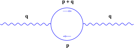
Figure 1: Generic one-loop diagram contributing to $\Omega_{i}$, with KK modes in the loop. Its value for $q^{2}=0$ can be read from eq.(16), (26) for one and two compact dimensions. See also Appendix A in [25].

$$\frac{1}{\alpha_{i}}\bigg{|}_{{1-loop}}\!\!\!=\frac{1}{\alpha_{i}}\bigg{|}_{{tree}}\!\!\!+\Omega_{i}^{*},\,\quad\Omega_{i}^{*}=\sum_{r}\sum_{\sigma=\lambda,\alpha}\!\!\Omega_{i}(\sigma),\,\quad\Omega_{i}(\sigma)\equiv\!\frac{\beta_{i}(\sigma)}{4\pi}\sum_{m\in{\bf Z}}^{\prime}\int_{0}^{\infty}\!\frac{dt}{t}\,e^{-\pi\,t\,M^{2}_{m}(\sigma)/\mu^{2}}\bigg{|}_{\textrm{reg.}}$$ (16)

where $\mu$ is a finite, non-zero mass parameter which enforces a dimensionless equation for $\Omega_{i}$. We would like to mention that the rhs formula for $\Omega_{i}$ is obtained by evaluating one loop diagrams for vanishing momentum ($q^{2}=0$), such as that of $\Pi(q^{2})$ shown in Figure 1, with a tower of Kaluza-Klein (KK) states each of mass $M_{m}(\sigma)$ ($m$ integer) present in the loop. For more technical details on how to obtain this expression for $\Omega_{i}$ see for example Appendix A in [25], or [21]. Note the distinction between the dependence (”running”) of the couplings on the momentum scale $q$ (see Figure 1) for large $q$ and given by $1/\alpha_{i}(q^{2})-1/\alpha_{i}(0)=(\Pi_{i}(q^{2})-\Pi_{i}(0))/\alpha_{i}(0)$, and their dependence on the UV cutoff (regulator) of the theory that we compute in this work for $q^{2}=0$ and given by $\Omega_{i}$. We will only briefly discuss the dependence on $q^{2}\!\not=\!0$ of the couplings, for a detailed analysis see [7, 20].

$\Omega_{i}(\sigma)$ is thus the contribution of an infinite tower of Kaluza-Klein modes associated with a state of charge $\sigma$ in the Weyl-Cartan basis and of mass “shifted” by $\rho(\sigma)$ real, with $\sigma=\lambda,\alpha$ the weights/roots belonging to the representation $r$. The “primed” sum over $m$ runs over all non-zero positive and negative integers (levels). The case when this sum is restricted to positive (negative) levels only will also be addressed. The effect of zero-modes is not included in $\Omega_{i}$ since their presence is in general model dependent. Thus their contribution should be added separately to $1/\alpha_{i}$. The important point to note is that while the sums over $r$ and $\sigma=\alpha,\lambda$ in eq.(16) depend on the field content and are thus model dependent, the integral and the sum in $\Omega_{i}$ over Kaluza-Klein modes of non-zero level depend only on the geometry of compactification. It is this integral and sum over KK levels which are difficult to perform exactly, and they are evaluated below.

Supersymmetry is not a necessary ingredient in formula (16). Supersymmetry is however present in many models with compact dimensions which consider MSSM-like models as the viable “low-energy” limit. Regarding the beta functions $\beta_{i}$ one has (we suppress the subscript $i$) that $\beta(\sigma)=k_{r}(\sigma_{I}\sigma^{I})/{\textrm{rk}G}$ for $\sigma$ belonging to representation $r$; $k_{r}=\{-11/3,2/3,1/3\}$ for adjoint representations, Weyl fermion and scalar respectively; $k_{r}$ essentially counts the degrees of freedom in the corresponding representations. The Dynkin index $T(r)=(\sum_{\sigma}\sigma_{I}\sigma^{I})_{r}/(\textrm{rk}G)$ where the sum is over all weights/roots $\sigma$ belonging to representation $r$, each occurring a number of times equal to its multiplicity [31]. With the definition $b_{i}(r)\equiv\sum_{\sigma}\beta_{i}(\sigma)$ for the weights $\sigma$ belonging to $r$ one has $b_{i}\!=\!-11/3\,T_{i}(A)+2/3\,T_{i}(R)+1/3\,T_{i}(S)$, to account for the adjoint, Weyl fermion in representation $R$ and scalar in representation $S$. In the supersymmetric case massive N=1 Kaluza-Klein states are organised as N=2 hypermultiplets (vector supermultiplets) with $b_{i}\!=\!2T_{i}(R)$ ($b_{i}\!=\!-2T_{i}(A)$).

The subscript “reg.” shows that formula (16) is not well defined in the UV region $t\rightarrow 0$, and a UV regularisation is required. We assume $M_{m}(\sigma)\not=0$ so no infrared (IR) regularisation (i.e. for $t\rightarrow\infty$) is needed. The use of a particular regularisation is in general dictated by the symmetries of the initial, higher dimensional theory. If a string embedding exists for this theory, a proper-time cutoff (PT) regularisation (although not gauge invariant) is in some cases the appropriate choice [14, 16]. In the absence of a fully specified such theory and to keep the analysis general we compute $\Omega_{i}$ in three regularisation schemes: DR, ZR and PT regularisation.

$\bullet$ Dimensional Regularisation (DR).

In this scheme $\Omega_{i}$ of eq.(16) has under the integral $1/t$ replaced by $1/t^{1+\epsilon}$ with $\epsilon\rightarrow 0$ the UV regulator. In such case $\mu$ is the arbitrary (finite, non-zero) mass scale introduced in the DR scheme in $d=4-\epsilon$ dimensions. The evaluation of $\Omega_{i}$ in DR is rather long and is presented in detail in Appendix A, eqs.(A-1) to (A). The calculation uses expansions in Hurwitz or Riemann zeta functions which do not necessarily involve a Poisson re-summation of the “original” KK levels. This has the advantage that one may be able to identify which of the original KK levels brings the leading contribution to $\Omega_{i}$. Using eqs.(9), (A-1), (A-2), (A) one finds for $\Omega_{i}$ in the DR scheme

$$\Omega_{i}{\bigg{|}_{DR}} = \!\frac{\beta_{i}(\sigma)}{4\pi}\sum_{m\in{\bf Z}}^{\prime}\int_{0}^{\infty}\!\frac{dt}{t^{1+\epsilon}}\,e^{-\pi\,t\,M^{2}_{m}(\sigma)/\mu^{2}}$$ (17)

$$= \frac{\beta_{i}(\sigma)}{4\pi}\,\bigg{\{}\,\frac{1}{\epsilon}-\ln\frac{(R\mu)^{2}}{\pi e^{\gamma}}-\ln\left|\,\frac{2\,\sin\pi({\rho_{\sigma}}+i\chi R)}{\rho_{\sigma}+i\chi R}\right|^{2}\bigg{\}}$$

The presence of the pole in $\epsilon$ accounts for an UV divergence. To find the scale dependence of this divergence in DR one may in general introduce a small/infrared mass shift $\chi$ of the momentum of the KK state. One would then expect the emergence in the final result of a term $\chi/\epsilon$ to account for a linear divergence (in scale), given the extra dimension present. However this procedure does not apply to the case with one compact dimension only. Therefore, unlike the case of two compact dimensions to be discussed later, the presence of the pole alone does not tell us the nature of the scale dependence of the UV divergence. Note also that a single state (such as the zero mode for example) gives a leading one-loop contribution proportional to $-1/\epsilon$, which is of the same form but of opposite sign to that found in eq.(17) for the whole Kaluza-Klein tower, excluding the zero-mode ! (compare ${\cal R}_{\epsilon}$ vs. finite ${\cal R}_{\epsilon}^{T}$ in eq.(A) of Appendix A). Further, this $-1/\epsilon$ pole due to a single state is also known to correspond in 4D to a UV divergence only logarithmic in scale (rather than linear). Note however that the change of the couplings with momentum $q$ in Fig.1 is indeed linear in the momentum scale $q$ and dominates if $(qR)^{2}\!\geq\!{\cal O}(1)$ [7, 20].

If $\rho_{\sigma}$ is a non-zero integer, there exists a level $n_{0}$ such as $M_{n_{0}}=\chi$ and then $\chi$ plays the role of an IR regulator in eqs.(16), (17), and ensures that the term $\ln[\sin\pi(\rho_{\sigma}+i\chi R)]$ remains finite. If $\rho_{\sigma}$, $\chi$ vanish the last term in (17) vanishes and one is left with the correction in the absence of the “twist” or Wilson line background $\rho_{\sigma}$.

In deriving $\Omega_{i}$ we summed over both positive and negative Kaluza-Klein levels, as shown in eq.(16). However, it is useful (particularly for orbifolds case) to analyse the effect of summing separately the contributions of the positive (negative) levels. In such a case the corresponding value of $\Omega_{i}$, denoted $\Omega_{i}^{+}$ ($\Omega_{i}^{-}$), is computed in a similar way. The result, derived in Appendix A, eqs.(A-18), (A-21) is

$$\Omega_{i}^{\pm}\bigg{|}_{DR} = \frac{\beta_{i}(\sigma)}{4\pi}\,\bigg{\{}\frac{1}{2\epsilon}\pm\frac{\rho_{\sigma}}{\epsilon}+\ln\Big{|}\Gamma(1\pm\rho_{\sigma}+i\chi R)\Big{|}^{2}-\ln(2\pi)-\Big{[}\frac{1}{2}\pm\rho_{\sigma}\Big{]}\ln\frac{(R\mu)^{2}}{\pi e^{\gamma}}\bigg{\}}$$ (18)

The divergent terms of $\Omega_{i}^{\pm}$ are then

$$\Omega_{i}^{\pm}\bigg{|}_{DR}\sim 1/(2\,\epsilon)\pm\rho_{\sigma}/\epsilon$$ (19)

The presence of the additional divergence $\rho_{\sigma}/\epsilon$ is triggered by a non-zero background/twist $\rho_{\sigma}$, and is cancelled in the sum $\Omega_{i}^{+}+\Omega_{i}^{-}$ of both positive and negative Kaluza-Klein levels, giving the overall result $\Omega_{i}$ in (17). If $\rho_{\sigma}$ has the value given in (2.1) and is thus proportional to the vev of $A_{z}$ and to $R$, then $\rho_{\sigma}/\epsilon$ may be regarded as a divergence linear in scale. It is also possible that in some models one may actually have $\rho_{\sigma}$ a constant, for example $\rho_{\sigma}=+1/2$, (or $-1/2$) then $\Omega_{i}^{-}$ ($\Omega_{i}^{+}$) are finite respectively, and the overall divergence in $\Omega_{i}=\Omega_{i}^{+}+\Omega_{i}^{-}$ comes entirely from $\Omega_{i}^{+}$ ($\Omega_{i}^{-}$) respectively! To conclude, the positive and negative Kaluza-Klein levels propagating in opposite directions in the compact dimension, with a non-zero background/twist $\rho_{\sigma}$, contribute by different amounts to the overall divergence of $\Omega_{i}$; in special cases the positive or negative levels alone give (one-loop) finite contributions ! This concludes our analysis in the DR scheme.

$\bullet$ $\zeta$-function Regularisation (ZR).

Alternatively, one can employ a $\zeta$-function regularisation of $\Omega_{i}$. In this case the correction is given (up to a factor $\beta_{i}(\sigma)/(4\pi)$), by the derivative of $\zeta$-function associated with the Laplacian, evaluated in origin. As detailed in Appendix B this means that $\Omega_{i}$ in this scheme is just the derivative with respect to $\epsilon$ of the value obtained in the DR scheme (divided by $\Gamma[-\epsilon]$), and evaluated for $\epsilon=0$. From eqs.(9), (16), (B), (B-7) one obtains the value of $\Omega_{i}$ in the ZR scheme

$$\Omega_{i}\bigg{|}_{ZR} = \frac{\beta_{i}(\sigma)}{4\pi}\frac{d}{d\epsilon}\bigg{\{}\frac{-\pi^{-\epsilon}}{\Gamma[-\epsilon]}\sum_{m\in{\bf Z}}^{\prime}\int_{0}^{\infty}\!\frac{dt}{t^{1+\epsilon}}\,e^{-\pi\,t\,M^{2}_{m}(\sigma)/\mu^{2}}\bigg{\}}\bigg{|}_{\epsilon\rightarrow 0}$$ (20)

$$= \frac{\beta_{i}(\sigma)}{4\pi}\,\bigg{\{}-\ln(R\mu)^{2}-\ln\left|\,\frac{2\,\sin\pi({\rho_{\sigma}}+i\chi R)}{\rho_{\sigma}+i\chi R}\right|^{2}\,\bigg{\}}$$

This result is similar to that found in the DR scheme, with the notable difference that there is no pole structure present. The above result is only logarithmically dependent on the mass scale $\mu$. As discussed in Appendix B, $\mu$ plays in the case of $\zeta$-function regularisation the role of the UV cutoff of the model. Finally, note that the contribution of a zero-mode - if included - would bring a similar dependence on $\mu$ but of opposite sign to cancel this dependence in the total sum (see also ${\cal R}_{\zeta}$ and ${\cal R}_{\zeta}^{T}$ in Appendix B).

One can show that the separate contributions to $\Omega_{i}$ of positive and negative Kaluza-Klein modes are different due to the asymmetry introduced by the Wilson lines or twist $\rho_{\sigma}$. The results are denoted $\Omega_{i}^{+}$ ($\Omega_{i}^{-}$) respectively, and are given by eq.(B-10)

$$\Omega_{i}^{\pm}\bigg{|}_{ZR} = \frac{\beta_{i}(\sigma)}{4\pi}\bigg{\{}\ln\Big{|}\Gamma[1\pm\rho_{\sigma}+i\chi R]\Big{|}^{2}-\ln(2\pi)-\Big{[}\frac{1}{2}\pm\rho_{\sigma}\Big{]}\ln{(R\mu)^{2}}\bigg{\}}$$ (21)

so the positive (negative) modes again bring a different UV behaviour ($\mu$ dependence)

$$\Omega_{i}^{\pm}\bigg{|}_{ZR}\sim-(1/2\pm\rho_{\sigma})\ln(R\mu)^{2}$$ (22)

For $\rho_{\sigma}$ just a constant, the $\rho_{\sigma}$-dependent term is just an additional logarithmic correction (in $\mu$ or $R$) to the couplings. However, in the case $\rho_{\sigma}$ is indeed due to a non-zero Wilson line vev (from initial $A_{z}$ gauge fields), a linear dependence of the couplings on this vev/scale emerges. This term can then have significant implications for the value of the gauge couplings. As it was the case in the DR scheme, such terms cancel in the sum of positive and negative modes’ contributions. A special case is $\rho_{\sigma}=\mp 1/2$ when the coefficient of the logarithmic UV divergence (in $\mu$) of $\Omega_{i}^{\pm}$ is vanishing, and $\Omega_{i}^{+}\,(\Omega_{i}^{-})$ has no $\mu$ dependence, with similarities to the DR case.

$\bullet$ Proper-time Regularisation (PT).

The above results for $\Omega_{i}$ can be compared to that obtained in the proper-time regularisation. In this regularisation $\Omega_{i}$ of eq.(16) has the lower limit of its integral set equal to $\xi>0$, where $\xi\!\rightarrow\!0$ is a dimensionless UV regulator. For details of the calculation of $\Omega_{i}$ in this scheme see Appendix C and ref. [16] (Appendix A-1). From eqs.(9), (C-1), (C-2), (C) and with the notation $\Lambda^{2}\equiv\mu^{2}/\xi$ one obtains for $\Omega_{i}$ in the PT scheme

$$\Omega_{i}\bigg{|}_{PT} = \frac{\beta_{i}(\sigma)}{4\pi}\sum_{m\in{\bf Z}}^{\prime}\int_{\xi}^{\infty}\!\frac{dt}{t}\,e^{-\pi\,t\,M^{2}_{m}(\sigma)/\mu^{2}}$$ (23)

$$= \frac{\beta_{i}(\sigma)}{4\pi}\,\bigg{\{}2R\Lambda-\ln\frac{(R\Lambda)^{2}}{\pi e^{\gamma}}-\ln\left|\,\frac{2\,\sin\pi({\rho_{\sigma}}\!+\!i\chi R)}{\rho_{\sigma}+i\chi R}\right|^{2}\bigg{\}}$$

The $\xi$ dependent terms combine naturally with the scale $\mu$ to define the UV cut-off $\Lambda$ of the model and one obtains a dependence on $\Lambda R$ only. Unlike the DR and ZR cases, a zero-mode contribution to the above result - if included - would not cancel the leading linear divergence (in $\Lambda\sim 1/\sqrt{\xi}$), but only the logarithmic one (for more details compare ${\cal R}_{\xi}$ and ${\cal R}_{\xi}^{T}$ in Appendix C, eq.(C)).

What is the meaning of the individual contributions to $\Omega_{i}$ ? Technical details show that the term $\ln|\rho_{\sigma}+i\chi R|$ is similar to a contribution corresponding to a massive Kaluza-Klein state of level zero. It may be interpreted as a one-loop effect of this state between the compactification scale $1/R$ and the scale set by the Wilson lines vev’s, $\sigma_{I}\!<\!A_{z}^{I}\!>\!$ with $\sigma$ accounting for a root/weight. The term $\ln[\sin(..)]$ in (23) is an effect due to “Poisson re-summed” (PR) Kaluza-Klein states (see eq.(G-5)), with the dominant contribution from the lower PR levels. Further, the logarithm $\ln(\Lambda R)$ can be thought of as a one loop effect from the compactification scale to the UV cutoff scale $\Lambda$. Finally, the term $\Lambda R$ is due to the presence of a large enough number of Kaluza-Klein modes which enable the Poisson re-summation. This term is due to the Poisson re-summed mode of zero-level. Thus one should expect $\Lambda R\gg 1$ because $\Lambda R$ approximates the number of Kaluza-Klein modes. In fact the PT result (23) is valid provided that

$$\max\left\{{1}/{R^{2}},\,\,\chi^{2},\,\,(<\!A_{z}^{I}\!>\!\sigma_{I})^{2}+\chi^{2}\right\}\ll\Lambda^{2}$$ (24)

derived from eq.(C-4) of Appendix C. Here we replaced $\rho_{\sigma}$ in terms of the vev’s of $A_{z}^{I}$ as in eq.(2.1). More generally, for arbitrary $\rho_{\sigma}$ this condition is

$$\max\left\{{1}/{R^{2}},\,\,\chi^{2},\,\,{\rho_{\sigma}^{2}}/{R^{2}}+\chi^{2}\right\}\ll\Lambda^{2}$$ (25)

Therefore the result in the PT scheme is valid if $R$ is large (in UV cutoff units) and if the gauge symmetry breaking vev’s or $(\rho_{\sigma}/R)^{2}$ and the mass scale $\chi^{2}$ have a sum much smaller than the UV cutoff. Note that these constraints are not shared by the DR or ZR counterparts computed above. This is important for in general to avoid a large UV sensitivity of the couplings one would like to have $\Lambda R\approx 1$ which is a region for which the PT result does not hold accurately. From comparing it with its DR counterpart, the presence of the pole $1/\epsilon$ of the latter may indicate that even if $\Lambda R$ is made smaller, of order unity, a UV divergence is still manifest. Finally, if one considered a string embedding of these models, the string counterpart of $\Lambda R\approx 1$ would be $M_{s}R\approx 1$ with $M_{s}$ the string scale. In this case string effects due to additional (winding) states not present in field theory may become important.

Comparing the three results for $\Omega_{i}$ obtained in these different regularisation schemes one observes that the finite (regulator independent) part is the same in all regularisations. This is a strong consistency check of the calculation. Regarding the divergent (i.e. regulator dependent) part, note that the $1/\epsilon$ term of DR is replaced in the PT cut-off regularisation by the $\xi$ ($\Lambda$) dependent term, accounting for a linear divergence. Note that the ZR counterpart has only (rather “mild”) a logarithmic UV divergence. Eqs.(17) to (23) generalise the results [25] for one compact dimension, in the presence of Wilson lines/twists $\rho_{\sigma}$.

3.2 Case 2. Two compact dimensions.

We consider now the case of a two dimensional compactification on $T^{2}$ with Wilson lines. With the structure of the mass spectrum of eq.(14) we again compute the general form of the correction to the 4D gauge couplings due to non-zero level Kaluza-Klein modes in the presence of Wilson lines. This correction can be applied to a large class of models [23]. Formally, the correction is

$$\Omega_{i}^{*}=\sum_{r}\sum_{\sigma=\lambda,\alpha}\Omega_{i}(\sigma),\qquad\quad\Omega_{i}(\sigma)\equiv\frac{\beta_{i}(\sigma)}{4\pi}\sum_{n_{1},n_{2}\in{\bf Z}}^{\prime}\int_{0}^{\infty}\frac{dt}{t}\,e^{-\pi\,t\,M^{2}_{n_{1},n_{2}}(\sigma)/\mu^{2}}\bigg{|}_{\textrm{reg.}}$$ (26)

Similarly to the case of one extra dimension, $\Omega_{i}$ is obtained by computing one loop diagrams evaluated for $q^{2}=0$ (Figure 1) with Kaluza-Klein states of mass $M_{n_{1},n_{2}}(\sigma)$ in the loop.

In the following we perform - for $\sigma$ fixed - the integral and the sums over $(n_{1},n_{2})\not=(0,0)$ in eq.(26). Any model dependence (beta functions $\beta_{i}(\sigma)$, sums over weights $\sigma$, representations $r$) can then easily be implemented on the final result for $\Omega_{i}^{*}$. The presence of the state $(n_{1},n_{2})=(0,0)$ is model dependent and its contribution should be considered separately. We again discuss the value of $\Omega_{i}$ in DR, ZR and PT regularisation schemes for the UV divergence ($t\rightarrow 0$) of eq.(26). We assume $M_{n_{1},n_{2}}\not=0$ for all integers, so no IR divergence (at $t\rightarrow\infty$) exists. However, if there exists a pair $(n_{1},n_{2})$ for which $M_{n_{1},n_{2}}=0$ see the results in the PT scheme of [15] and the discussion in the DR scheme to follow.

$\bullet$ Dimensional Regularisation (DR).

In the DR scheme $\Omega_{i}$ is defined with $1/t$ under its integral replaced by $1/t^{1+\epsilon}$ where $\epsilon\rightarrow 0$ is the UV regulator. The calculation is rather technical and is presented in Appendix D, eq.(D-1) to (D-5), where the sums over $n_{1,2}$ and integral in (26) are evaluated. Using eqs.(14), (26), (D-2), (D-5) and (G-4), one obtains $\Omega_{i}$ in the DR scheme

$$\Omega_{i}\bigg{|}_{DR} = \frac{\beta_{i}(\sigma)}{4\pi}\sum_{n_{1},n_{2}\in{\bf Z}}^{\prime}\int_{0}^{\infty}\frac{dt}{t^{1+\epsilon}}\,e^{-\pi\,t\,M^{2}_{n_{1},n_{2}}(\sigma)/\mu^{2}}$$ (27)

$$= \frac{\beta_{i}(\sigma)}{4\pi}\bigg{\{}\frac{1}{\epsilon}-\ln\frac{T_{2}U_{2}}{\pi e^{\gamma}}-\ln\bigg{|}\frac{\vartheta_{1}({\rho_{2,\sigma}}-U{\rho_{1,\sigma}}|U)}{(\rho_{2,\sigma}-U\rho_{1,\sigma})\,\,\eta(U)}\,e^{i\pi U\rho^{2}_{1,\sigma}}\bigg{|}^{2}\bigg{\}}$$

The special functions $\eta,\,\vartheta_{1}$ are defined in Appendix G. The pole $1/\epsilon$ accounts for divergences up to quadratic level. How can we see this? By introducing a small (mass)² shift $\mu^{2}\delta$ to $M_{n_{1},n_{2}}^{2}$, ($\delta$ dimensionless, $\delta\ll 1$), i.e. $M_{n_{1},n_{2}}^{2}\rightarrow M_{n_{1},n_{2}}^{2}+\mu^{2}\delta$ under the integral in (26) and computing the integral in this more general case one obtains for $\Omega_{i}$, in addition to the divergence $1/\epsilon$, a contribution $\pi\delta T_{2}/\epsilon$. This is a quadratic divergence in scale ($T_{2}$ “contains” a $\mu^{2}$) that $1/\epsilon$ term effectively signals in eq.(27) and (D-5). For additional technical details see Appendix D, eq.(D), (D-8). The emergence of the additional scale dependent contribution $\pi\delta T_{2}/\epsilon$ is to be contrasted with what happened in DR in the one extra dimension case already discussed, where a small mass shift did not introduce a scale dependence of the UV divergence. This is due to the different UV behaviour of models with one (or odd number of) and two (or even number of) compact dimensions, respectively. Note that in the special case when there exists a pair $(n_{1},n_{2})$ such as $M_{n_{1},n_{2}}=0$, an IR regulator - in addition to the UV one - is required in eq.(26), (27) to ensure the convergence of the integral at $t\rightarrow\infty$. The aforementioned shift $\mu^{2}\delta$ of the KK masses would in such special case act as an IR regulator in (26) and one would obtain in (27) a term $\pi\delta T_{2}/\epsilon$ which represents an IR-UV “mixing” term between the IR sector ($\delta$) and UV sector ($\epsilon$) of the theory. For a discussion on this UV-IR mixing see [15, 20] where its string theory interpretation is also presented. Finally, considerations similar to those for one extra dimension apply for the separate role of negative or positive Kaluza-Klein levels, respectively.

$\bullet$ $\zeta$-function Regularisation (ZR).

In this scheme $\Omega_{i}$ is related to the derivative of the Zeta-function associated with the Laplacian, as discussed in Appendix E. In fact $\Omega_{i}$ in ZR is the derivative with respect to $\epsilon$ of $\Omega_{i}$ in DR divided by $\Gamma[-\epsilon]$, and evaluated for $\epsilon=0$. Using eqs.(14), (E-5), (E-6), (G-4) one finds $\Omega_{i}$ in the ZR scheme

$$\Omega_{i}\bigg{|}_{ZR} = \frac{\beta_{i}(\sigma)}{4\pi}\frac{d}{d\epsilon}\bigg{\{}\frac{-\pi^{-\epsilon}}{\Gamma[-\epsilon]}\sum_{n_{1},n_{2}\in{\bf Z}}^{\prime}\int_{0}^{\infty}\frac{dt}{t^{1+\epsilon}}\,e^{-\pi\,t\,M^{2}_{n_{1},n_{2}}(\sigma)/\mu^{2}}\bigg{\}}\bigg{|}_{\epsilon\rightarrow 0}$$ (28)

$$= \frac{\beta_{i}(\sigma)}{4\pi}\bigg{\{}-\ln[T_{2}U_{2}]-\ln\bigg{|}\frac{\vartheta_{1}({\rho_{2,\sigma}}-U{\rho_{1,\sigma}}|U)}{(\rho_{2,\sigma}-U\rho_{1,\sigma})\,\,\eta(U)}\,e^{i\pi U\rho^{2}_{1,\sigma}}\bigg{|}^{2}\bigg{\}}$$

This result has a form similar to that in the DR scheme from which the pole structure has been subtracted. The $\mu$ scale dependence “hidden” in $T_{2}$ should in this case be regarded as the UV cutoff as discussed in Appendix E, eq.(E-2). In this scheme there is thus only a logarithmic dependence on the UV cutoff. Finally, the finite part is similar to that obtained in the DR scheme. It would be of phenomenological interest to know which higher dimensional theories would require such a regularisation, since in this case the UV cut-off dependence of the couplings is milder and the models would then have less amount of sensitivity to this cut-off scale, possibly similar to that of MSSM-like models.

$\bullet$ Proper-time Regularisation (PT).

Finally, for a comparison we include here the value of $\Omega_{i}$ in the proper-time cutoff regularisation scheme (PT) [16]. In this scheme $\Omega_{i}$ of (26) is defined with a (dimensionless) cutoff $\xi\!\rightarrow\!0$ in the lower limit of its integral which acts as an UV regulator. After a long calculation one obtains the result (for details see eqs.(26), (F-2), (F-5), (G-4) and also eq.(52) in [16])

$$\!\!\!\Omega_{i}\bigg{|}_{PT} = \frac{\beta_{i}(\sigma)}{4\pi}\sum_{n_{1},n_{2}\in{\bf Z}}^{\prime}\int_{\xi}^{\infty}\frac{dt}{t}\,e^{-\pi\,t\,M^{2}_{n_{1},n_{2}}(\sigma)/\mu^{2}}$$ (29)

$$= \frac{\beta_{i}(\sigma)}{4\pi}\bigg{\{}\frac{T_{2}}{\xi}-\ln\frac{[(T_{2}/\xi)\,U_{2}]}{\pi e^{\gamma}}-\ln\bigg{|}\frac{\vartheta_{1}({\rho_{2,\sigma}}-U{\rho_{1,\sigma}}|U)}{(\rho_{2,\sigma}-U\rho_{1,\sigma})\,\eta(U)}\,e^{i\pi U\rho^{2}_{1,\sigma}}\bigg{|}^{2}\bigg{\}}$$

Eq.(29) is valid if (see eq.(F-6) and definition (12))

$$\max\left\{\frac{1}{R_{1}},\,\,\frac{1}{R_{2}\sin\theta},\,\,<\!A_{z}^{I}\!>\!\sigma_{I},\,\,<\!A_{\bar{z}}^{I}\!>\!\sigma_{I}\right\}\ll\Lambda,\qquad\Lambda^{2}\equiv\frac{\mu^{2}}{\xi}$$ (30)

This condition requires “large” compactification radii (in UV cutoff units) and symmetry breaking vev’s much smaller than $\Lambda$. Here we replaced $\rho_{i,\sigma}$ in terms of the vev’s of $A_{z}^{I}$, eq.(12) but for arbitrary $\rho_{i,\sigma}$ this condition is: $\max\{1/R_{1},1/R_{2}\sin\theta,|\rho_{1,\sigma}|/R_{1},|\rho_{2,\sigma}-U\rho_{1,\sigma}|/(R_{2}\sin\theta)\}\ll\Lambda$.

Eq.(29) shows the presence of a UV quadratic divergent term also known as “power-like” threshold, given by $T_{2}/\xi=\Lambda^{2}R_{1}R_{2}\sin\theta$ where $\Lambda^{2}\sim 1/\xi$ is the UV cutoff scale. A logarithmic correction is also present, $\ln(T_{2}/\xi)=\ln(\Lambda R_{1}R_{2}\sin\theta)$, as well as a $\ln U_{2}=\ln(R_{2}\sin\theta/R_{1})$ part. The remaining term in $\Omega_{i}$ includes effects due to non-zero $\rho_{\sigma}$ which bring in a finite, regulator independent correction.

The field theory result (29) has a great advantage over its DR and ZR counterparts in that it allows a straightforward comparison with the heterotic string result with Wilson lines. Here we refer to the 4D N=1 heterotic string orbifolds with N=2 sectors (of unrotated $T^{2}$) and Wilson lines [12] when this string result is considered in the limit of large compactification radii/area (in string units) [16], as required by eq.(30). The UV regulator $\xi\sim 1/\Lambda^{2}$ has a natural counterpart in the (heterotic) string in $\alpha^{\prime}\sim 1/M_{s}^{2}$ ($M_{s}$ is the string scale). Therefore, $T_{2}/\xi$ of (29) has a counterpart at the string level in $T_{2}/\alpha^{\prime}$, where $T_{2}/\alpha^{\prime}$ is the (imaginary part of the) Kähler structure moduli. With the correspondence of the fundamental lengths in field and string theory respectively, $\xi\leftrightarrow\alpha^{\prime}$, the result (29) is indeed similar [16] to the limit of large radii of the heterotic string result [12]. Such agreement provides support for this regularisation scheme in the field theory approach, although it is not gauge invariant. String theory also brings additional corrections, non-perturbative on the field theory side (world-sheet instantons) but their effect is exponentially suppressed ${\cal O}(e^{-T_{2}/\alpha^{\prime}})$ [12]. For more details on the exact link with the corrections to the gauge couplings due to the heterotic string with Wilson lines present, see [16].

The effective field theory result (29) has an interesting limit, that of vanishing Wilson lines vev’s or “twists” $\rho_{i,\sigma}$. For $\rho_{i,\sigma}\!\rightarrow\!0$ ($\sigma$ fixed) after using the relations in eq.(G), (G-2) one finds

$$\Omega_{i}\bigg{|}_{PT}(\rho_{i,\sigma}\!\rightarrow\!0)=-\frac{\beta_{i}(\sigma)}{4\pi}\ln\Big{[}4\pi e^{-\gamma}\,e^{-{T_{2}}/{\xi}}\,\,{({T_{2}}/{\xi})}\,\,U_{2}\,|\eta(U)|^{4}\Big{]},\qquad{T_{2}}/{\xi}=\Lambda^{2}R_{1}R_{2}\sin\theta$$ (31)

For two compact dimensions this result generalises the “power-law” corrections (in the UV cutoff) of ref.[25], by including the dependence on $U=R_{2}/R_{1}e^{i\theta}$.

The field theory result (31) is itself the exact limit [14, 15] of “large $R_{1,2}$” (in string units) of a similar result in 4D N=1 heterotic string orbifolds with N=2 sectors (of unrotated $T^{2}$) without Wilson lines [9]. The only difference between $\Omega_{i}$ of (31) and the above limit of the string result [9] is that the leading term $T_{2}/\xi$ in $\Omega_{i}$ has a coefficient which depends on the regulator choice ($\xi$) while in string case at “large $R_{1,2}$” the leading term is $(\pi/3)T_{2}/\alpha^{\prime}$. With the correspondence $\xi\leftrightarrow\alpha^{\prime}$ mentioned before, the exact matching of these two terms thus requires a re-definition of the PT regulator $\xi\rightarrow(3/\pi)\,\xi$ or equivalently $\Lambda^{2}\rightarrow\pi/3\,\Lambda^{2}$. Such specific normalisation of $\xi$ (or $\Lambda$) cannot be motivated on field theory grounds only.

It is interesting to mention that imposing on the field theory result (31) one of the string symmetries $T\leftrightarrow U$ or $T\leftrightarrow 1/T$, enables one to recover the full heterotic string result [9] from that derived using only field theory methods. Thus one may obtain full string results by using only field theory methods supplemented by some of the symmetries of the string, not respected by the field theory approach, but imposed on the final field theory result. For more details on the exact link with the heterotic string without Wilson lines see [14, 15]. This ends our discussion on the corrections in the PT regularisation scheme and their relation to string theory.

Comparing the results for $\Omega_{i}$ in the three regularisation schemes eqs.(27) to (29), one notices that the finite (regulator independent) part of $\Omega_{i}$ is the same in all cases which is a consistency check of the calculation. An important point to mention is that the result in the PT scheme has the constraint that the compactification radii be large (in UV cutoff units). The results in the DR and ZR schemes show that the finite part of the one-loop correction has the value found without such restrictions.

Regarding the divergent part of the one-loop corrections, this is effectively dictated by the regularisation choice one has to make, in agreement with the symmetries of the model. Our discussion above shows that for two compact dimensions the PT regularisation is indeed appropriate in calculations seeking the link with their string counterparts. Further, the $\zeta$-function regularisation leads to an UV divergence which is milder (logarithmic) than in the PT scheme with possible phenomenological implications. This is important because models with “power-like” regime require in general a significant amount of fine-tuning [32]. It is difficult to justify, without the knowledge of the full higher dimensional theory, in which case the $\zeta$-function regularisation is the right choice. The results of eqs.(27) to (31) generalise, in the presence of Wilson lines, early results [25] for the radiative corrections from two compact dimensions.

The one-loop corrections obtained in the DR, ZR or PT schemes have strong similarities with their one-dimensional counterparts, eqs.(17) to (23) with $T_{2}U_{2}$ and $\rho_{2,\sigma}-U\rho_{1,\sigma}$ of eqs.(27) to (29) replaced in the one-dimensional case by $R\mu$ and $\rho_{\sigma}$ respectively, while $\ln(\vartheta_{1}/\eta)$ has as counterpart in the one-dimensional case the term $\ln[\sin\pi(\rho+i\chi)]$. A similar term appears in compactification on $G_{2}$ manifolds [19] suggesting that this latter correction is rather generic.

We end with a remark on possible phenomenological implications. The result for $\Omega_{i}$ has a divergence which depends - as expected - on the regularisation choice. Since this is a non-renormalisable theory, a natural question is whether one can make a prediction without the knowledge of the fundamental, underlying theory which would otherwise dictate the regularisation to use. If the gauge group G after orbifolding is a grand unified group which is further broken by Wilson lines to a SM-like group, the coefficient of the (regularisation dependent) divergent terms found in $\Omega_{i}^{*}$ is the same for all group factors into which $G$ is broken ($G$-invariant). If so, such UV divergent terms of $\Omega_{i}^{*}$ can then be absorbed into the redefinition of the initial 4D tree level coupling of the group G. The newly defined coupling can be regarded as the 4D “MSSM-like” unified coupling. Further, the remaining, finite part of $\Omega_{i}^{*}$ brings a splitting term to this coupling, due to Wilson lines vev $\rho_{\sigma}$, but independent on the UV cutoff (regularisation). Finally, the “MSSM-like” massless states not included so far would bring the usual logarithmic correction (UV scale dependent). This raises the possibility of allowing MSSM-like logarithmic unification even for “large” compact dimensions, and the aforementioned splitting of couplings would “mimic” (at a scale of the order of the compactification scale) what could be seen from a 4D point of view as further running up to a high unification scale, such as that of the MSSM ($\approx 2\times 10^{16}$ GeV) or higher.

4 Conclusions

The general structure of radiative corrections to gauge couplings was investigated in generic 4D models with one and two dimensional compactifications in the presence of Wilson lines. The analysis was based on the following observation. Although one-loop corrections are dependent on the exact field content of the model, for the compactifications considered one can still perform in a general case, the one-loop integral and the infinite sums over (non-zero) Kaluza-Klein levels associated with a given state, component of a multiplet. This leaves the much simpler analysis of determining which states have associated Kaluza-Klein towers, to a model-by-model analysis.

The evaluation of the one-loop radiative corrections from compact dimensions summed up the individual effects of non-zero-level Kaluza-Klein modes. Although the models are non-renormalisable, the calculation was kept general by considering the radiative effects in three regularisation schemes: dimensional, zeta-function and proper-time cutoff regularisations for the UV divergences and the exact link among these results was investigated. The results in DR and $\zeta$-function regularisation schemes are very similar with the notable difference that the (UV) pole structure of the DR scheme ($1/\epsilon$) is not present in the $\zeta$-function regularisation. This applies to both one and two extra dimensions cases. In the ZR scheme for $\Omega_{i}$ only a logarithmic divergence in the UV cutoff scale is present. This is important, since it provides an amount of sensitivity of the radiative corrections to this scale smaller than that of other regularisations, which may be relevant for phenomenology. In the DR and ZR schemes the finite part of the results is valid for either large or small compactification radii, for both one and two compact dimensions cases.

In proper-time regularisation the leading divergences of the radiative corrections are for one and two compact dimensions linear and quadratic in scale, respectively. The finite (regulator independent) part is the same as in the DR and zeta-function regularisation, which is a strong consistency check of the calculation. The result in the proper-time regularisation is only valid for “large” compactification radii (in UV cutoff units), constraint not shared by the results in the DR and ZR schemes. The effect of zero-modes (whose existence is model dependent) can easily be added to the results we obtained. In specific cases they may even cancel the divergence from the entire KK tower of non-zero modes. Finally, we also discussed the cases when for special values of the background/twists $\rho_{\sigma}$, one obtains one-loop finite results for the corrections due to positive or negative modes alone.

There remains the question of which regularisation scheme to use in (non-renormalisable) models with compact dimensions. Explicit calculations and comparison with the (heterotic) string show that proper-time cut-off regularisation is in exact quantitative agreement with the limit of large compactification radii of the string results. This applies to the case of two compact dimensions which contribute to the radiative corrections to the gauge couplings. Therefore this regularisation is an appropriate choice for computing radiative corrections for the purpose of establishing the link with results from string theory. However, this regularisation may be of limited use in field theory since is not gauge invariant. For the case of one compact dimension the lack of string results prevents one from making a similar statement, and the choice of regularisation should follow the usual guidelines such as its compatibility with the symmetries of the model.

We addressed the possibility of making phenomenological predictions which are independent of the UV divergence of the radiative corrections which, in the case of a grand unified group G broken by Wilson lines vev’s/twist $\rho_{\sigma}$, can be absorbed in the redefinition of the tree level coupling. This leaves a splitting of the couplings at the compactification scale possibly compatible with what can be regarded in a 4D (renormalisable) theory as further “running” up to a high, MSSM-like unification scale.

The paper provides all the technical details necessary in models with one and two compact dimensions which examine the one-loop corrections to the gauge couplings from Kaluza-Klein thresholds in the presence of Wilson lines. Although we discussed only the dependence of the corrections on the UV cutoff/regulator, the paper provides the technical results for investigating the change of the gauge couplings with respect to the (momentum) scale $q$ as well. Extensive mathematical details of regularisations of integrals and series present in one-loop corrections due to compact dimensions were provided in the Appendix. Our results can be applied with minimal changes to many one- and two-dimensional orbifolds with Wilson lines, by making appropriate re-definitions of the parameters of the models, such as the compactification radii ($R$), the twist of the initial fields with respect to the compact dimensions or the Wilson lines vev’s ($\rho$).

5 Acknowledgements

The author thanks Graham Ross for discussions on this topic and suggestions on a previous version of this paper. He also thanks Stefan Förste, Joel Giedt, Fernando Quevedo and Martin Walter for discussions on related topics. This work was supported by a post-doctoral research fellowship from the Particle Physics and Astronomy Research Council PPARC (UK).

6 Appendix

We provide general results for series of integrals present in one-loop corrections to the gauge couplings, evaluated in DR, $\zeta$-function and proper-time cut-off regularisations, for one and two compact dimensions (see also Appendix A-4 in [16]). Notation used: A “primed” sum $\sum_{m}^{\prime}f(m)$ is a sum over $m\in{\bf Z}-\{0\}$; $\sum_{m,n}^{\prime}f(m,n)$ is a sum over all pairs of integers $(m,n)$ excluding $(m,n)\!=\!(0,0)$.

A One compact dimension in Dimensional Regularisation (DR)

$\bullet$ A.(1).      We compute the following integral

$${\cal R}_{\epsilon}\equiv\int_{0}^{\infty}\frac{dt}{t^{1+\epsilon}}\sum^{\prime}_{m\in{\bf Z}}e^{-\pi\,t\,[(m+\rho)^{2}\beta+\delta]},\qquad\quad\delta\geq 0,\,\,\beta\!>\!0.$$ (A-1)

$\Omega_{i}$ of eq.(17) is then given by

$$\Omega_{i}\Big{|}_{DR}=\beta_{i}(\sigma)/(4\pi)\,\,{\cal R}_{\epsilon}(\beta\!\rightarrow\!1/(R\mu)^{2};\,\delta\!\rightarrow\!(\chi/\mu)^{2};\,\rho\rightarrow\rho_{\sigma})$$ (A-2)

Proof: Consider first $0<\delta/\!\beta\!\leq 1$. With the notation $\rho=[\rho]+\Delta_{\rho}$, $[\rho]\in{\bf Z}$, $0\leq\!\Delta_{\rho}\!<1$ one has

$$\!\!\!\!\!{\cal R}_{\epsilon} = \int_{0}^{\infty}\frac{dt}{t^{1+\epsilon}}\bigg{[}-e^{-\pi\,t\,\beta\rho^{2}}+e^{-\pi\,t\,\beta\Delta_{\rho}^{2}}+\sum_{n\in{\bf Z}}^{\prime}e^{-\pi\,t\,(n+\Delta_{\rho})^{2}\beta}\bigg{]}\,e^{-\pi\,t\,\delta}$$ (A-3)

$$= \Gamma[-\epsilon]\pi^{\epsilon}\bigg{\{}(\delta+\beta\Delta_{\rho}^{2})^{\epsilon}-(\delta+\beta\rho^{2})^{\epsilon}+\bigg{[}\sum_{n>0}[\beta(n+\Delta_{\rho})^{2}+\delta]^{\epsilon}+(\Delta_{\rho}\rightarrow-\Delta_{\rho})\bigg{]}\bigg{\}}$$

$$= \Gamma[-\epsilon]\pi^{\epsilon}\big{[}(\delta+\beta\Delta_{\rho}^{2})^{\epsilon}-(\delta+\beta\rho^{2})^{\epsilon}]+\Gamma[-\epsilon](\pi\beta)^{\epsilon}\bigg{[}\zeta[-2\epsilon,1+\Delta_{\rho}]+\zeta[-2\epsilon,1-\Delta_{\rho}]\bigg{]}$$

$$+ (\pi\beta)^{\epsilon}\sum_{k\geq 1}\frac{\Gamma[k-\epsilon]}{k!}\bigg{[}\frac{-\delta}{\beta}\bigg{]}^{k}\,\bigg{\{}\zeta[2k-2\epsilon,1+\Delta_{\rho}]+(\Delta_{\rho}\rightarrow-\Delta_{\rho})\bigg{\}},\quad 0<\delta/\beta\leq 1$$

which is convergent under conditions shown. In the last step we used the binomial expansion [29]

$$\sum_{n\geq 0}[a(n+c)^{2}+q]^{-s}=a^{-s}\sum_{k\geq 0}\frac{\Gamma[k+s]}{k\,!\,\Gamma[s]}\bigg{[}\frac{-q}{a}\bigg{]}^{k}\zeta[2k+2s,c],\qquad 0<q/a\leq 1$$ (A-4)

Here $\zeta[q,a]$ with $a\not=0,-1,-2,\cdots$ is the Hurwitz zeta function, (with $\zeta[q,a]=\sum_{n\geq 0}(a+n)^{-q}$ for $\textrm{Re}(q)>1$). Hurwitz zeta-function has one singularity (simple pole) at $q=1$ and $\zeta[q,1]=\zeta[q]$ with $\zeta[q]$ the Riemann zeta function. Further, using eq.(A-3) and the identity

$$\zeta[q,a]=a^{-q}+\zeta[q,a+1]$$

we obtain that

$$\!\!\!\!\!\!\!\!\!\!\!\!\!\!\!\!{\cal R}_{\epsilon}\!\! = \!\pi^{\epsilon}\Gamma[-\epsilon]\big{[}(\delta+\beta\Delta_{\rho}^{2})^{\epsilon}-(\delta+\beta\rho^{2})^{\epsilon}]+(\pi\beta)^{\epsilon}\Gamma[-\epsilon]\bigg{[}\zeta[-2\epsilon,1+\Delta_{\rho}]+\zeta[-2\epsilon,1-\Delta_{\rho}]\bigg{]}$$ (A-5)

$$+ \sum_{k\geq 1}\bigg{[}\frac{-\delta}{\beta}\bigg{]}^{k}\frac{1}{k}\bigg{[}\zeta[2k,1+\Delta_{\rho}]+\zeta[2k,2-\Delta_{\rho}]+(1-\Delta_{\rho})^{-2k}\bigg{]}$$

$$= \pi^{\epsilon}\Gamma[-\epsilon]\big{[}(\delta+\beta\Delta_{\rho}^{2})^{\epsilon}-(\delta+\beta\rho^{2})^{\epsilon}]+(\pi\beta)^{\epsilon}\Gamma[-\epsilon]\bigg{[}\zeta[-2\epsilon,1+\Delta_{\rho}]+\zeta[-2\epsilon,1-\Delta_{\rho}]\bigg{]}$$

$$- \!\ln\frac{|\sin\pi[\Delta_{\rho}+i(\delta/\beta)^{\frac{1}{2}}]|^{2}}{\pi^{2}(\Delta_{\rho}^{2}+\delta/\beta)}-2\ln\bigg{[}\Gamma[1-\Delta_{\rho}]\,\Gamma[1+\Delta_{\rho}]\bigg{]}$$

provided that

$$0<\frac{\delta}{\beta}\leq 1;\qquad\frac{\delta}{\beta}<(1+\Delta_{\rho})^{2},\qquad\frac{\delta}{\beta}<(2-\Delta_{\rho})^{2}$$ (A-6)

Since $\Delta_{\rho}\!<\!1$ we conclude that (A-5) is valid if the first condition (the strongest) is respected:

$$0<\frac{\delta}{\beta}\leq 1;$$ (A-7)

In the last step of deriving eq.(A-5) for each of the series in Zeta functions we used [30]

$$\sum_{k\geq 1}\frac{t^{2k}}{k}\,\zeta[2k,a]=\ln\frac{\Gamma[a+t]\,\Gamma[a-t]}{\Gamma[a]^{2}};\qquad|t|<|a|$$ (A-8)

with $t=i(\delta/\beta)^{\frac{1}{2}}$, $a=1+\Delta_{\rho},\,2-\Delta_{\rho}$ and from which the last two conditions in (A-6) emerged. Finally, in the last step in (A-5) we also used

$$\prod_{\pm}\Gamma[1\pm x\pm iy]=\frac{\pi^{2}(x^{2}+y^{2})}{|\sin\pi(x+iy)|^{2}},\qquad x,y\,\,\,\textrm{real}.$$ (A-9)

where the product runs over all 4 combinations of plus/minus signs in the argument of $\Gamma$ functions. Eq.(A-9) can be easily proved using that $\Gamma[1-z]\,\Gamma[1+z]=\pi z/\sin\pi z$.

In eq.(A-5) we now evaluate the $\epsilon$ dependent part for $\epsilon\rightarrow 0$ by using (see for example [28])

$$\zeta[-2\epsilon,q] = \frac{1}{2}-q-2\epsilon\,\frac{d}{dz}\zeta[z,q]|_{z=0}+{\cal O}(\epsilon^{2})$$

$$\frac{d}{dz}\zeta[z,q]|_{z=0} = \ln\Gamma[q]-\frac{1}{2}\ln(2\pi),\qquad\Gamma[-\epsilon]=-\frac{1}{\epsilon}-\gamma+{\cal O}(\epsilon),$$

$$x^{\epsilon} = 1+\epsilon\ln x+{\cal O}(\epsilon^{2})$$ (A-10)

We finally find from eq.(A-5), (A-7), (A) that (if $\rho\in{\bf Z}^{*}$, $\delta=0$ is excluded)

$${\cal R}_{\epsilon}=\int_{0}^{\infty}\frac{dt}{t^{1+\epsilon}}\sum^{\prime}_{m\in{\bf Z}}e^{-\pi\,t\,[(m+\rho)^{2}\beta+\delta]}=\frac{1}{\epsilon}-\ln\frac{|2\,\sin\pi(\Delta_{\rho}+i(\delta/\beta)^{\frac{1}{2}})|^{2}}{\pi e^{\gamma}\,\beta\,(\rho^{2}+\delta/\beta)},\qquad 0\leq\delta/\beta\leq 1$$ (A-11)

$\bullet$ A.(2).    We now evaluate ${\cal R}_{\epsilon}$ for the case $\delta/\beta>1$ (with notation $\rho\equiv[\rho]+\Delta_{\rho}$, $[\rho]\in{\bf Z}$, $0\leq\!\Delta_{\rho}\!<1$)

$${\cal R}_{\epsilon}=\int_{0}^{\infty}\frac{dt}{t^{1+\epsilon}}\sum^{\prime}_{m\in{\bf Z}}e^{-\pi\,t\,[(m+\rho)^{2}\beta+\delta]} = \int_{0}^{\infty}\frac{dt}{t^{1+\epsilon}}\bigg{[}\sum_{n\in{\bf Z}}e^{-\pi\,t\,(n+\Delta_{\rho})^{2}\beta}-e^{-\pi\,t\,\beta\rho^{2}}\bigg{]}\,e^{-\pi\,t\,\delta}$$ (A-12)

$$= \Gamma[-\epsilon]\pi^{\epsilon}\bigg{[}\sum_{n\in{\bf Z}}[\beta(n+\Delta_{\rho})^{2}+\delta]^{\epsilon}-(\delta+\beta\rho^{2})^{\epsilon}\bigg{]}$$

We further use the well-known expansion given below (for details see for example (4.13) in [29])

$$\!\!\!\!\!\!\!\sum_{n\in{\bf Z}}[a(n+c)^{2}+q]^{-s} = \sqrt{\pi}\bigg{[}\frac{q}{a}\bigg{]}^{\frac{1}{2}}\frac{\Gamma[s-1/2]}{\Gamma[s]}\,q^{-s}$$ (A-13)

$$+ \frac{4\pi^{s}}{\Gamma[s]}\bigg{[}\frac{q}{a}\bigg{]}^{\frac{1}{4}}q^{-{s}/{2}}a^{-{s}/{2}}\sum_{n=1}^{\infty}n^{s-1/2}\cos(2\pi n\,c)\,K_{s-1/2}(2\pi n\sqrt{q/a})$$

with $a\!>\!0$, $c\!\not=\!0,-1,-2,\cdots$ and which is rapidly convergent for $q/a>1$. $K_{w}$ is the modified Bessel function of index $w$. The first term proportional to $q/a$ gives the leading contribution; the remaining ones give “instanton-like” corrections. This result is then used to evaluate (A-12). Compare (A-13) rapidly convergent for $q/a>1$ with (A-4) valid for $q/a<1$. Alternatively, instead of (A-13) one can simply use a Poisson re-summation in (A-12) and the definition of the modified Bessel functions to reach the same result. With $s=-\epsilon$ in (A-13) and with

$$\Gamma[-\epsilon]=-\frac{1}{\epsilon}-\gamma+{\cal O}(\epsilon),\qquad K_{-\frac{1}{2}}(z)=\sqrt{\frac{\pi}{2z}}e^{-z}$$ (A-14)

one finds from (A-12) and (A-13)

$${\cal R}_{\epsilon}=\int_{0}^{\infty}\frac{dt}{t^{1+\epsilon}}\sum^{\prime}_{m\in{\bf Z}}e^{-\pi\,t\,[(m+\rho)^{2}\beta+\delta]}=\frac{1}{\epsilon}-\ln\frac{\left|\,2\,\sin\pi(\Delta_{\rho}+i(\delta/\beta)^{\frac{1}{2}})\right|^{2}}{\pi e^{\gamma}\,(\delta+\beta\rho^{2})},\quad\textrm{if}\,\,\,\delta/\beta>1$$ (A-15)

To see the complementarity of (A-11) and (A-15) note that the latter is not valid for $\delta=0$ since (A-13) is not valid in that case.

In conclusion from eqs.(A-11), (A-15) we have that

$${\cal R}_{\epsilon} \equiv \int_{0}^{\infty}\frac{dt}{t^{1+\epsilon}}\sum^{\prime}_{m\in{\bf Z}}e^{-\pi\,t\,[(m+\rho)^{2}\beta+\delta]}=\frac{1}{\epsilon}-\ln\frac{\left|2\,\sin\pi(\rho+i(\delta/\beta)^{\frac{1}{2}})\right|^{2}}{\pi e^{\gamma}\,(\beta\rho^{2}+\delta)},\quad\delta\!\geq\!0,\,\beta\!>\!0.$$

$${\cal R}^{T}_{\epsilon} \equiv \int_{0}^{\infty}\frac{dt}{t^{1+\epsilon}}\sum_{m\in{\bf Z}}e^{-\pi\,t\,[(m+\rho)^{2}\beta+\delta]}=-\ln\left|\,2\,\sin\pi(\rho+i(\delta/\beta)^{\frac{1}{2}})\right|^{2},\quad\delta\!\geq\!0,\,\beta\!>\!0.$$ (A-16)

In eq.(A) we used the properties of the sine function to replace $\Delta_{\rho}$ by $\rho$. The pole $1/\epsilon$ cancels between zero-mode and non-zero modes’ contributions. Eq.(A) was used in the text eq.(17).

$\bullet$ A.(3).      We compute the integral

$${\cal R}_{\epsilon}^{+}\equiv\int_{0}^{\infty}\frac{dt}{t^{1+\epsilon}}\sum_{m>0}e^{-\pi\,t\,[(m+\rho)^{2}\beta+\delta]},\qquad\quad\delta\geq 0,\,\,\beta\!>\!0.$$ (A-17)

which sums positive modes only. ${\cal R}_{\epsilon}^{-}$ which sums negative modes only is then ${\cal R}_{\epsilon}^{-}={\cal R}_{\epsilon}^{+}(\rho\rightarrow-\rho)$. $\Omega_{i}^{\pm}$ mentioned in the text, eq.(19) and corresponding to summing only positive (negative) Kaluza-Klein modes is then given by

$$\Omega_{i}^{\pm}\bigg{|}_{DR}\equiv\beta_{i}(\sigma)/({4\pi})\,\,{\cal R}_{\epsilon}^{\pm}\Big{(}\beta\!\rightarrow\!1/(R\mu)^{2};\,\delta\!\rightarrow\!(\chi/\mu)^{2};\,\rho\rightarrow\rho_{\sigma}\Big{)}$$ (A-18)

The calculation proceeds almost identically to A.(1). The result is:

$${\cal R}_{\epsilon}^{+}=\frac{1}{2\epsilon}+\frac{\rho}{\epsilon}+\ln\Big{|}\Gamma[1+\rho+i(\delta/\beta)^{1/2}]\Big{|}^{2}-\ln(2\pi)+\Big{[}\frac{1}{2}+\rho\Big{]}\ln(\pi\beta e^{\gamma})$$ (A-19)

which shows that a new divergence $\rho/\epsilon$ is present. One can easily verify that

$${\cal R}_{\epsilon}^{+}+{\cal R}_{\epsilon}^{-}={\cal R}_{\epsilon}$$ (A-20)

with ${\cal R}_{\epsilon}$ given in (A). This shows that the divergence $\rho/\epsilon$ of separate contributions from the positive and negative modes respectively is cancelled in their sum which equals ${\cal R}_{\epsilon}$. While ${\cal R}_{\epsilon}$ corresponds to states propagating in both directions in the compact dimension in the “background” $\rho$, ${\cal R}_{\epsilon}^{\pm}$ account for effects propagating in one direction only.

Similar properties exist for the full one-loop radiative corrections $\Omega_{i}^{\pm}$ given below, corresponding to positive and negative modes respectively. The radiative correction in DR due to positive (negative) modes only is

$$\Omega_{i}^{\pm}\bigg{|}_{DR} \equiv \frac{\beta_{i}(\sigma)}{4\pi}\,{\cal R}_{\epsilon}^{\pm}\Big{(}\beta\!\rightarrow\!1/(R\mu)^{2};\,\delta\!\rightarrow\!(\chi/\mu)^{2};\,\rho\rightarrow\rho_{\sigma}\Big{)}$$ (A-21)

$$= \frac{\beta_{i}(\sigma)}{4\pi}\,\left\{\frac{1}{2\epsilon}\pm\frac{\rho_{\sigma}}{\epsilon}+\ln\Big{|}\Gamma(1\pm\rho_{\sigma}+i\chi R)\Big{|}^{2}-\ln(2\pi)+\Big{[}\frac{1}{2}\pm\rho_{\sigma}\Big{]}\ln\frac{\pi e^{\gamma}}{(R\mu)^{2}}\right\}$$

One has that $\Omega_{i}^{+}+\Omega_{i}^{-}=\Omega_{i}$ with $\Omega_{i}$ as in (17). The “linear” divergence $\rho_{\sigma}/\epsilon$ cancels between positive and negative modes’ contributions.

B One compact dimension in $\zeta$-function regularisation (ZR).

$\bullet$ Here we define/evaluate $\Omega_{i}$ of eq.(20) in the ZR scheme. The one-loop correction to the gauge couplings in Zeta-function regularisation is defined by (proportional to) the derivative of the Zeta function associated with the Laplacian on the compact manifold and evaluated in 0. To see this note that $\zeta$-function of the Laplacian (eigenvalues $\lambda_{m}>0$) is defined as

$$\zeta_{\Delta}[s]\equiv\sum_{m}^{\prime}\frac{1}{\lambda_{m}^{s}}=\frac{1}{\Gamma[s]}\sum_{m}^{\prime}\int_{0}^{\infty}\frac{dt}{t^{1-s}}\,e^{-\lambda_{m}\,t}$$ (B-1)

where we used that

$$Q^{-s}=\frac{1}{\Gamma[s]}\int_{0}^{\infty}\frac{dt}{t^{1-s}}\,e^{-Q\,t},\qquad Q>0$$ (B-2)

From (B-1) the formal derivative of the zeta function $\zeta_{\Delta}^{{}^{\prime}}[0]$ is an infinite sum of individual logarithms of $\lambda_{m}$. With $\lambda_{m}$ expressed in some mass units $\mu$, ($\lambda_{m}=M_{m}^{2}/\mu^{2}$) one has the formal result

$$\frac{d\zeta_{\Delta}[s]}{ds}\bigg{|}_{s=0}=-\sum_{m}^{\prime}\ln\lambda_{m}=\sum_{m}^{\prime}\ln(\mu/M_{m})^{2}$$ (B-3)

and the link of $\Omega_{i}$ with the one-loop corrections is obvious; $\mu$ acts as effective field theory UV cutoff.

From eq.(B-1) we have

$${\cal R}_{\zeta}\equiv\frac{d\zeta_{\Delta}[s]}{ds}\bigg{|}_{s=0}=\frac{d}{ds}\,\bigg{[}\frac{1}{\Gamma[s]}\sum^{\prime}_{m}\int_{0}^{\infty}\frac{dt}{t^{1-s}}\,e^{-\lambda_{m}\,t}\bigg{]}_{s=0}$$ (B-4)

which relates $\zeta$-function regularisation of an operator to its value in the DR scheme. One can also include the contribution of the zero mode $m=0$ (if $\lambda_{0}\not=0$) in the definition of $\zeta_{\Delta}[s]$. Accordingly ${\cal R}_{\zeta}$ changes and is relabelled ${\cal R}_{\zeta}^{T}$.

With $\lambda_{m}=(m+\rho)^{2}\beta+\delta$ as general eigenvalues of Laplacian for one-dimensional case (see eq.(9)) with boundary conditions given in the text, and using the results of eq.(A)

$${\cal R}_{\epsilon} \equiv \int_{0}^{\infty}\frac{dt}{t^{1+\epsilon}}\sum^{\prime}_{m\in{\bf Z}}e^{-\pi\,t\,[(m+\rho)^{2}\beta+\delta]}=\frac{1}{\epsilon}-\ln\frac{\left|2\,\sin\pi(\rho+i(\delta/\beta)^{\frac{1}{2}})\right|^{2}}{\pi e^{\gamma}\,(\delta+\beta\rho^{2})}$$

$${\cal R}^{T}_{\epsilon} \equiv \int_{0}^{\infty}\frac{dt}{t^{1+\epsilon}}\sum_{m\in{\bf Z}}e^{-\pi\,t\,[(m+\rho)^{2}\beta+\delta]}=-\ln\left|\,2\,\sin\pi(\rho+i(\delta/\beta)^{\frac{1}{2}})\right|^{2}$$ (B-5)

we finally find

$$\!\!\!\!\!\!\!\!{\cal R}_{\zeta}\!\! \!\!\!\!=\!\!\!\! \!\!-\frac{d}{d\epsilon}\bigg{\{}\frac{\pi^{-\epsilon}}{\Gamma[-\epsilon]}\,R_{\epsilon}\,\bigg{\}}_{\epsilon=0}\!\!\!=\!-\ln\frac{|2\,\sin\pi(\rho+i(\delta/\beta)^{\frac{1}{2}})|^{2}}{(\delta+\beta\rho^{2})}$$

$$\!\!\!\!\!\!\!\!\!\!\!{\cal R}_{\zeta}^{T}\!\! \!\!\!\!=\!\!\!\! \!\!-\frac{d}{d\epsilon}\bigg{\{}\frac{\pi^{-\epsilon}}{\Gamma[-\epsilon]}\,R_{\epsilon}^{T}\bigg{\}}_{\epsilon=0}\!\!\!\!=\!-\ln\left|\,2\,\sin\pi(\rho+i(\delta/\beta)^{\frac{1}{2}})\right|^{2}$$ (B-6)

Comparing the results of the last two sets of equations, one notices that (up to a constant) the result in $\zeta$-function regularisation is equal to that in DR from which the pole contribution was subtracted.

Eqs.(B-1), (B-4) (B) allow us to evaluate $\Omega_{i}$ of eq.(20). This is given by

$$\Omega_{i}\bigg{|}_{ZR}\equiv{\beta_{i}(\sigma)}/(4\pi)\,\,{\cal R}_{\zeta}\left(\delta\rightarrow\chi^{2}/\mu^{2},\,\,\beta\rightarrow 1/(R\mu)^{2},\,\,\rho\rightarrow\rho_{\sigma}\right)$$ (B-7)

According to eq.(B-3) $\mu$ should be regarded as the effective field theory UV cutoff.

$\bullet$ Using the DR results eq.(A-17) of summing over positive (negative) modes only

$${\cal R}_{\epsilon}^{\pm} \equiv \int_{0}^{\infty}\frac{dt}{t^{1+\epsilon}}\sum_{m>0}e^{-\pi\,t\,[(m\pm\rho)^{2}\beta+\delta]}$$ (B-8)

$$= \frac{1}{2\epsilon}\pm\frac{\rho}{\epsilon}+\ln\Big{|}\Gamma[1\pm\rho+i(\delta/\beta)^{1/2}]\Big{|}^{2}-\ln(2\pi)+\Big{[}\frac{1}{2}\pm\rho\Big{]}\ln(\pi\beta e^{\gamma})$$

one finds the associated $\zeta$-regularised result for positive (negative) modes’ contribution

$${\cal R}_{\zeta}^{\pm}\equiv-\frac{d}{d\epsilon}\bigg{\{}\frac{\pi^{-\epsilon}}{\Gamma[-\epsilon]}{\cal R}_{\epsilon}^{\pm}\bigg{\}}=\ln\Big{|}\Gamma[1\pm\rho+i(\delta/\beta)^{1/2}]\Big{|}^{2}-\ln(2\pi)+\Big{[}\frac{1}{2}\pm\rho\Big{]}\ln\beta$$ (B-9)

The effect of positive (negative) modes on the gauge couplings in $\zeta$-function regularisation is then

$$\Omega_{i}^{\pm}\bigg{|}_{ZR} \equiv \frac{\beta_{i}(\sigma)}{4\pi}\,{\cal R}_{\zeta}^{\pm}\,\bigg{(}\delta\rightarrow\chi^{2}/\mu^{2};\,\beta\rightarrow 1/(R\mu)^{2};\,\rho\rightarrow\rho_{\sigma}\bigg{)}$$ (B-10)

$$= \frac{\beta_{i}(\sigma)}{4\pi}\left\{\ln\Big{|}\Gamma[1\pm\rho_{\sigma}+i\chi R]\Big{|}^{2}-\ln(2\pi)+\Big{[}\frac{1}{2}\pm\rho_{\sigma}\Big{]}\ln\frac{1}{(R\mu)^{2}}\right\}$$

This result was used in eq.(22).

C One compact dimension in proper-time regularisation (PT).

$\bullet$ Here we provide technical details used to derive the result of eq.(23). In the proper-time cutoff regularisation, the generic structure of the one-loop corrections is

$${\cal R}_{\xi} \equiv \int_{\xi}^{\infty}\frac{dt}{t}\,\sum^{\prime}_{n\in{\bf Z}}e^{-\pi t\,[(n+\rho)^{2}\,\beta+\delta]},\qquad\xi\rightarrow 0,\,\,\,(\xi>0);\,\,\delta\geq 0,\,\,\beta>0.$$ (C-1)

$\Omega_{i}$ of eq.(23) is then given by

$$\Omega_{i}\bigg{|}_{PT}\equiv\beta_{i}(\sigma)/(4\pi)\,\,{\cal R}_{\xi}(\beta\rightarrow 1/(R\mu)^{2};\,\rho\!\rightarrow\!\rho_{\sigma};\,\delta\!\rightarrow\!\chi^{2}/\mu^{2};\,\xi\rightarrow\!\xi)$$ (C-2)

To obtain ${\cal R}_{\xi}$ we use eq.(A-9) of Appendix A-1 of [16]. One has

$${\cal R}_{\xi} = \int_{\beta\xi}^{\infty}\frac{dt}{t}\sum_{n\in{\bf Z}}^{\prime}e^{-\pi t[(n+\rho)^{2}+\delta/\beta]}$$ (C-3)

$$= \ln\bigg{[}(\rho^{2}+\delta/\beta)\pi e^{\gamma}\bigg{]}-\ln\frac{e^{-2/\sqrt{\xi\beta}}}{\xi\beta}-\ln\left|\,2\,\sin\pi(\Delta_{\rho}+i(\delta/\beta)^{\frac{1}{2}})\right|^{2}$$

with $\Delta_{\rho}$ defined after eq.(A-2) and which is valid if:

$$\xi\beta\ll\bigg{\{}1;\frac{1}{\pi\delta/\beta};\frac{1}{\pi(\rho^{2}+\delta/\beta)}\bigg{\}}$$ (C-4)

One concludes that

$$\!{\cal R}_{\xi} \!\equiv\! \sum^{\prime}_{n\in{\bf Z}}\int_{\xi}^{\infty}\frac{dt}{t}\,e^{-\pi t\,[(n+\rho)^{2}\,\beta+\delta]}=-\ln\frac{e^{-2/\sqrt{\xi\beta}}}{\xi}\!-\!\ln\frac{\left|\,2\,\sin\pi(\rho\!+\!i(\delta/\beta)^{\frac{1}{2}})\right|^{2}}{[\pi e^{\gamma}(\delta+\beta\rho^{2})]}$$

$${\cal R}_{\xi}^{T} \!\equiv\! \sum_{n\in{\bf Z}}\int_{\xi}^{\infty}\frac{dt}{t}\,e^{-\pi t\,[(n+\rho)^{2}\,\beta+\delta]}=\frac{2}{\sqrt{\xi\beta}}-\ln\left|\,2\,\sin\pi(\rho+i(\delta/\beta)^{\frac{1}{2}})\right|^{2}$$ (C-5)

with condition (C-4). In the above equations we replaced $\Delta_{\rho}$ by $\rho$.

Note that adding the zero-mode to ${\cal R}_{\xi}$ does not cancel the leading linear divergence unlike the cases of DR or ZR schemes! To understand the differences among the various regularisation schemes it is useful to compare the above result of the PT regularisation eq.(C), (C-4) with that of DR regularisation eq.(A), and that of $\zeta$-function regularisation eq.(B).

Eq.(C) was used in the text, eq.(23).

D Two compact dimensions in Dimensional Regularisation (DR).

$\bullet$ For two compact dimensions we evaluate the integral:

$$L_{\epsilon}\equiv\int_{0}^{\infty}\frac{dt}{t^{1+\epsilon}}\sum_{m_{1},m_{2}\in{\bf Z}}^{\prime}e^{-\pi t\,\tau|m_{2}+\rho_{2}-U(m_{1}+\rho_{1})|^{2}},\qquad\quad\tau>0;\quad U=U_{1}+iU_{2}$$ (D-1)

$\Omega_{i}$ of eq.(27) is then given by

$$\Omega_{i}\bigg{|}_{DR}=\beta_{i}(\sigma)/(4\pi)\,\,L_{\epsilon}\big{(}\tau\rightarrow 1/(T_{2}U_{2}),\,\rho_{i}\rightarrow\rho_{i,\sigma}\big{)}$$ (D-2)

Proof: To compute $L_{\epsilon}$ we use the Poisson re-summation eq.(G-5), so the integrand of $L_{\epsilon}$ becomes

$$\sum_{m_{1},m_{2}}^{\prime}e^{-\pi t\,\tau|m_{2}+\rho_{2}-U(m_{1}+\rho_{1})|^{2}} = \sum_{m_{2}}^{\prime}e^{-{\pi\,t\,\tau}|m_{2}+\rho_{2}-U\rho_{1}|^{2}}+\sum_{m_{1}}^{\prime}\sum_{m_{2}\in{\bf Z}}e^{-{\pi\,t\,\tau|m_{2}+\rho_{2}-U(m_{1}+\rho_{1})|^{2}}}$$ (D-3)

$$= \sum_{m_{2}}^{\prime}e^{-\pi\,t\,\tau|m_{2}+\rho_{2}-U\rho_{1}|^{2}}+\frac{1}{\sqrt{t\,\tau}}\sum_{m_{1}}^{\prime}e^{-\pi t\,\tau U_{2}^{2}\,(m_{1}+\rho_{1})^{2}}$$

$$+ \frac{1}{\sqrt{t\,\tau}}\sum_{m_{1}}^{\prime}\sum_{\tilde{m}_{2}}^{\prime}e^{-\frac{\pi{\tilde{m}_{2}}^{2}}{t\,\tau}-\pi t\,\tau U_{2}^{2}\,(m_{1}+\rho_{1})^{2}+2\pi i{\tilde{m}_{2}}(\rho_{2}-U_{1}(\rho_{1}+m_{1}))}$$

A prime on the double sum in the lhs indicates that the mode $(m_{1},m_{2})\!\not=\!(0,0)$ is excluded. If $\rho_{1}$ is non-integer the three series in the rhs of (D-3) can be integrated separately over $(0,\infty$) to find

$$L_{\epsilon} = L_{1}+L_{2}+L_{3},\qquad\qquad\textrm{where}$$

$$\!\!L_{1} \equiv \int_{0}^{\infty}\frac{dt}{t^{1+\epsilon}}\sum_{m_{2}}^{\prime}e^{-\pi\,t\,\tau|m_{2}+\rho_{2}-U\rho_{1}|^{2}}=\frac{1}{\epsilon}-\ln|\,2\sin\pi(\rho_{2}-U\rho_{1})\,|^{2}+\ln\Big{[}\pi\,\tau e^{\gamma}|\rho_{2}-U\rho_{1}|^{2}\Big{]}$$

$$\!\!L_{2} \equiv \frac{1}{\sqrt{\tau}}\int_{0}^{\infty}\!\frac{dt}{t^{3/2+\epsilon}}\sum_{m_{1}}^{\prime}e^{-\pi t\,\tau\,U_{2}^{2}\,(m_{1}+\rho_{1})^{2}}=2\pi U_{2}\Big{[}|\rho_{1}|+\frac{1}{6}-\Delta_{\rho_{1}}+\Delta_{\rho_{1}}^{2}\Big{]},$$

$$\!\!L_{3} \equiv \frac{1}{\sqrt{\tau}}\int_{0}^{\infty}\!\frac{dt}{t^{3/2+\epsilon}}\sum_{m_{1}}^{\prime}\sum_{\tilde{m}_{2}}^{\prime}e^{-\pi\tilde{m}_{2}^{2}\frac{1}{t\,\tau}-\pi t\,\tau U_{2}^{2}(m_{1}+\rho_{1})^{2}+2\pi i\tilde{m}_{2}(\rho_{2}-U_{1}(\rho_{1}+m_{1}))}$$ (D-4)

$$= \ln\Big{|}2\sin\pi(\rho_{2}-U\rho_{1})\Big{|}^{2}-2\pi U_{2}\Big{[}|\rho_{1}|+\frac{1}{6}-\Delta_{\rho_{1}}\Big{]}-\ln\bigg{|}\frac{\vartheta_{1}(\Delta_{\rho_{2}}-U\Delta_{\rho_{1}}|U)}{\eta(U)}\bigg{|}^{2}$$

where $\Delta_{y}$ denotes the positive definite fractional part of $y$ defined as $y=[y]+\Delta_{y}$, $0<\Delta_{y}<1$, with $[y]$ an integer number. $\vartheta_{1}(z|\tau)$ and $\eta(U)$ are special functions defined in the Appendix, eqs.(G-3).

To evaluate $L_{1}$ we used eq.(A-15) with the following replacements for the arguments of this equation: $\beta\rightarrow\tau$, $\rho\rightarrow\rho_{2}-U_{1}\rho_{1}$ and $\delta\rightarrow\tau U_{2}^{2}\rho_{1}^{2}$. To compute $L_{2}$ we used the results of Appendix A of ref.[16], eq.(A-22) or more generally eqs.(A-43), (A-45). Regarding $L_{3}$, taking the limit $\epsilon\rightarrow 0$ is allowed under the integral before performing the integral itself or the two sums. This is justified by technical calculations (not shown) which prove that $L_{3}$ is bound by an expression which has no poles in $\epsilon\rightarrow 0$. This is actually expected because the integrand is well defined for $t\rightarrow 0$ or $t\rightarrow\infty$ when $\epsilon=0$. After setting $\epsilon=0$ the integral equals that evaluated in eqs.(A-28) to (A-31) in Appendix (A-3) of ref [16].

Adding together $L_{1},\,L_{2},\,L_{3}$ we find for $U=U_{1}+iU_{2}$, $\tau>0$

$$L_{\epsilon} \equiv \int_{0}^{\infty}\frac{dt}{t^{1+\epsilon}}\sum_{m_{1},m_{2}\in{\bf Z}}^{\prime}e^{-\pi t\,\tau|m_{2}+\rho_{2}-U(m_{1}+\rho_{1})|^{2}}$$ (D-5)

$$= \frac{1}{\epsilon}+\ln[\pi\,\tau e^{\gamma}]-\ln\bigg{|}\frac{\vartheta_{1}(\Delta_{\rho_{2}}-U\Delta_{\rho_{1}}|U)}{[\rho_{2}-U\rho_{1}]\,\eta(U)}\bigg{|}^{2}+2\pi U_{2}\Delta_{\rho_{1}}^{2},\qquad\tau>0$$

Further, one can make the replacement $\Delta_{\rho_{i}}\!\rightarrow\!\rho_{i}$, due to the identity given in eq.(G-4). Eq.(D-5) was used in the text, eq.(27).

Using the properties of $\vartheta_{1}$ (Appendix G) one also finds an interesting limit of $L_{\epsilon}$ for $\rho_{1}\!=\rho_{2}\!=0$:

$$L_{\epsilon}(\rho_{1,2}=0)\,\,\equiv\,\int_{0}^{\infty}\frac{dt}{t^{1+\epsilon}}\sum_{m_{1},m_{2}\in{\bf Z}}^{\prime}e^{-\pi t\,\tau|m_{2}-Um_{1}|^{2}}\,=\,\frac{1}{\epsilon}+\ln\big{[}\tau e^{\gamma}/(4\pi)\big{]}-\ln|\eta(U)|^{4},\quad\tau>0.$$ (D-6)

in agreement with eq.(B-12) of ref. [14]. Note that the contribution of the $(0,0)$ mode - if added to $L_{\epsilon}$ - would cancel the pole $1/\epsilon$ and $\ln\tau|\rho_{2}-U\rho_{1}|$ term above.

$\bullet$ One important observation is in place here. To find the scale dependence of the divergence ($1/\epsilon$) of $L_{\epsilon}$ in the DR scheme one can introduce a small/infrared (mass)² parameter $\mu^{2}\delta$ ($\delta$ dimensionless, $\delta>0$) in addition to the (mass)² of the Kaluza-Klein states in the exponent in eqs.(26), (D-1). This amounts to multiplying the integrand in eq.(26) by $e^{-\pi t\,\delta\,\mu^{2}}$ or that in (D-1) by $e^{-\pi t\,\delta}$. After a long algebra one obtains the following change for $L_{1}$, $L_{2}$, $L_{3}$:

$$L_{1} \rightarrow L_{1}^{\prime}=L_{1},\qquad\qquad\qquad\quad\textrm{if}\quad\delta\rightarrow 0$$

$$L_{2} \rightarrow L_{2}^{\prime}=L_{2}+\frac{\pi\delta}{\epsilon}\frac{1}{\tau U_{2}},\qquad\,\textrm{if}\quad\delta\rightarrow 0$$

$$L_{3} \rightarrow L_{3}^{\prime}=L_{3},\qquad\qquad\quad\qquad\textrm{if}\quad\delta\rightarrow 0$$ (D-7)

As a result

$$L^{\prime}_{\epsilon} \equiv \int_{0}^{\infty}\frac{dt}{t^{1+\epsilon}}\sum_{m_{1,2}\in{\bf Z}}^{\prime}e^{-\pi t\,\tau|m_{2}+\rho_{2}-U(m_{1}+\rho_{1})|^{2}-\pi\delta t}$$ (D-8)

$$= L_{1}^{\prime}+L_{2}^{\prime}+L_{3}^{\prime}\,\,\,\,=\,\,\,\,L_{\epsilon}+\frac{\pi\delta}{\epsilon}\frac{1}{\tau U_{2}},\quad\textrm{with}\quad\delta\rightarrow 0;\quad\delta,\tau>0;\quad U=U_{1}+iU_{2}$$

with $L_{\epsilon}$ given in (D-5). Therefore a divergence is emerging $\delta/(\tau U_{2}\epsilon)$, induced by the change of $L_{2}$. With $\tau=1/(T_{2}U_{2})$ the divergence is proportional to $T_{2}/\epsilon$, and is quadratic in mass, given the definition of $T_{2}$. It is similar to that of proper-time regularisation ($T_{2}/\xi$), see Appendix F. Note that $L_{2}^{\prime}$ which brings in this term is a contribution from both compact dimensions, as Kaluza-Klein modes’ effects from one dimension and Poisson re-summed Kaluza-Klein zero-modes of the second compact dimension. Also note a particular and useful limit of eq.(D-8), that with $\rho_{1}=\rho_{2}=0$.

$\bullet$ For future reference we also give the result of computing the integral:

$$L^{*}_{\epsilon}\equiv\int_{0}^{\infty}\!\!\!\frac{dt}{t^{1+\epsilon}}\!\!\sum_{m_{1},m_{2}\in{\bf Z}}^{\prime}e^{-\pi\,t\,\tau\,|Um_{1}-m_{2}|^{2}-\pi\,t\,\delta}\qquad\tau>0;\,\,\delta\geq 0,\,\,\,U\equiv U_{1}+i\,U_{2}.$$ (D-9)

Proof: Following the steps in eq.(D-3) one has $L^{*}_{\epsilon}=L^{*}_{1}+L_{2}^{*}+L_{3}^{*}$ with

$$L^{*}_{1} \equiv \int_{0}^{\infty}\!\frac{dt}{t^{1+\epsilon}}\,\sum_{m_{2}}^{\prime}e^{-\pi\,t\,\tau\,m_{2}^{2}-\pi\,\delta\,t}=\frac{1}{\epsilon}-\ln\bigg{[}\frac{|2\sinh\pi(\delta/\tau)^{1/2}|^{2}}{\pi\,e^{\gamma}\,\delta}\bigg{]}$$

$$L^{*}_{2} \equiv \frac{1}{\sqrt{\tau}}\int_{0}^{\infty}\!\frac{dt}{t^{3/2+\epsilon}}\,\sum_{m_{1}}^{\prime}e^{-\pi\,t\,\tau\,U_{2}^{2}\,m_{1}^{2}-\pi\,\delta\,t}$$

$$= \frac{\pi U_{2}}{3}+\frac{\pi\,\delta}{\epsilon\,\tau U_{2}}+\frac{\pi\,\delta}{\tau\,U_{2}}\ln\bigg{[}4\pi\,e^{-\gamma}\tau U_{2}^{2}\bigg{]}+2\sqrt{\pi}\,U_{2}\sum_{k\geq 1}\frac{\Gamma[k+1/2]}{(k+1)!}\bigg{[}\frac{-\delta}{\tau\,U_{2}^{2}}\bigg{]}^{k+1}\zeta[2k+1]$$

$$L^{*}_{3} \equiv \frac{1}{\sqrt{\tau}}\int_{0}^{\infty}\!\frac{dt}{t^{3/2+\epsilon}}\sum_{m_{1}}^{\prime}\sum_{\tilde{m}_{2}}^{\prime}e^{-\pi\,{\tilde{m}_{2}}^{2}/(t\,\tau)-\pi\,t\,\tau\,U_{2}^{2}m_{1}^{2}-2i\pi\tilde{m}_{2}m_{1}U_{1}-\pi\,\delta\,t}$$ (D-10)

$$= -\ln\prod_{m_{1}\geq 1}{\bigg{|}1-e^{-2\pi(\delta/\tau+U_{2}^{2}m_{1}^{2})^{1/2}}\,e^{2i\pi U_{1}m_{1}}\bigg{|}^{4}}$$

For $L_{1}^{*}$ we used eq.(A), for $L_{2}^{*}$ see eq.(B-11) to (B-15) in Appendix B of [15]. For $L_{3}^{*}$ one may set $\epsilon=0$ (no poles at $t\rightarrow 0$ or $t\rightarrow\infty$) and use the integral representation of Bessel function $K_{1/2}$ with $K_{1/2}(z)$ given in (A-14). Adding together the above contributions one has

$$L^{*}_{\epsilon}=\frac{1}{\epsilon}+\frac{\pi\delta}{\epsilon}\frac{1}{\tau U_{2}}-\ln\bigg{[}4\pi e^{-\gamma}\frac{1}{\tau}\,|\eta(U)|^{4}\bigg{]}+\frac{\pi\delta}{\tau U_{2}}\ln(4\pi e^{-\gamma}\,\tau\,U_{2}^{2})-2\ln\frac{\sinh\pi(\delta/\tau)^{\frac{1}{2}}}{\pi(\delta/\tau)^{\frac{1}{2}}}+{\cal W}\bigg{(}\frac{\delta}{\tau}\bigg{)}$$ (D-11)

with the constraint $0<\delta\,|U|^{2}/(U_{2}^{2}\tau)\leq 1$, $0<\delta/(\tau U_{2}^{2})\leq 1$. Also ${\cal W}(y\rightarrow 0)\rightarrow 0$ and is defined as

$${\cal W}(y)\equiv 2\sqrt{\pi}U_{2}\sum_{k\geq 1}\frac{\Gamma[k+1/2]}{(k+1)!}\bigg{[}\frac{-y}{U_{2}^{2}}\bigg{]}^{k+1}\!\!\!\zeta[2k+1]-\ln\!\!\prod_{m_{1}\geq 1}\frac{{|1-e^{-2\pi(y+U_{2}^{2}m_{1}^{2})^{1/2}+2i\pi U_{1}m_{1}}|^{4}}}{{|1-e^{2i\pi Um_{1}}|^{4}}}$$ (D-12)

E Two compact dimensions in $\zeta$-function regularisation (ZR)

$\bullet$ Here we derive the result for $\Omega_{i}$ of eq.(28) in the text. The one-loop correction to gauge couplings in $\zeta$-function regularisation is proportional to the derivative of $\zeta$-function associated with the Laplacian on the compact manifold, evaluated in 0 (See also the discussion in Appendix B).

$\zeta$-function of the Laplacian (eigenvalues $\lambda_{m,n}>0$) is defined as

$$\zeta_{\Delta}[s]\equiv\sum_{m,n\in{\bf Z}}^{\prime}\frac{1}{\lambda_{m,n}^{s}}=\frac{1}{\Gamma[s]}\sum_{m,n\in{\bf Z}}^{\prime}\int_{0}^{\infty}\frac{dt}{t^{1-s}}\,e^{-\lambda_{m,n}\,t}$$ (E-1)

where we used eq.(B-2) and the “primed” sum excluded the $(0,0)$ mode. Note that as in the one extra-dimension case, one can express $\lambda_{m,n}$ in some mass units $\mu$, $\lambda_{m,n}=M_{m,n}^{2}/\mu^{2}$ and one has that, formally

$$\frac{d\zeta_{\Delta}[s]}{ds}\bigg{|}_{s=0}=-\sum_{m,n}^{\prime}\ln\lambda_{m,n}=\sum_{m,n}^{\prime}\ln(\mu/M_{m,n})^{2}$$ (E-2)

and one can see the link of this derivative with the one-loop radiative corrections, given by a sum over individual logarithmic corrections, with $\mu$ acting as the UV cutoff of the model. Up to a beta function coefficient, eq.(E-2) is also in agreement with the formal expression in eq.(1).

From eq.(E-1) one has

$$L_{\zeta}\equiv\frac{d\zeta_{\Delta}[s]}{ds}\bigg{|}_{s=0}=\frac{d}{ds}\,\bigg{[}\frac{1}{\Gamma[s]}\sum^{\prime}_{m,n\in{\bf Z}}\int_{0}^{\infty}\frac{dt}{t^{1-s}}\,e^{-\lambda_{m}\,t}\bigg{]}_{s=0}$$ (E-3)

which relates $\zeta$-function regularisation of an operator to (the derivative of) its DR result.

With general eigenvalues of Laplacian for the two-dimensional case (see eq.(14))

$$\lambda_{m,n}=\tau|(m_{2}+\rho_{2})-U(m_{1}+\rho_{1})|^{2},\qquad\tau>0$$ (E-4)

and using $L_{\epsilon}$ of eq.(D-5), one has

$$L_{\zeta} = -\frac{d}{d\epsilon}\left\{\frac{\pi^{-\epsilon}}{\Gamma[-\epsilon]}L_{\epsilon}\right\}=\ln[\tau]-\ln\bigg{|}\frac{\vartheta_{1}(\Delta_{\rho_{2}}-U\Delta_{\rho_{1}}|U)}{[{\rho_{2}}-U{\rho_{1}}]\,\eta(U)}\bigg{|}^{2}+2\pi U_{2}\Delta_{\rho_{1}}^{2}$$ (E-5)

One can further replace $\Delta_{\rho_{i}}\!\rightarrow\!\rho_{i}$, due to the identity in eq.(G-4). The result in $\zeta$-function regularisation is equal to that in DR from which the contribution of the pole was subtracted.

$\bullet$ Eq.(E-5) was used to evaluate $\Omega_{i}$ in the text eq.(28) with

$$\Omega_{i}\bigg{|}_{ZR}=\beta_{i}(\sigma)/(4\pi)\,\,L_{\zeta}\left(\tau\!\rightarrow 1/(T_{2}U_{2}),\,\rho_{i}\rightarrow\rho_{i,\sigma}\right)$$ (E-6)

F Two compact dimensions in proper-time regularisation (PT).

$\bullet$ In the PT regularisation one evaluates (see the Appendix in ref.[16])

$$L_{\xi} \equiv \int_{\xi}^{\infty}\frac{dt}{t}\sum_{m_{1,2}\in{\bf Z}}^{\prime}e^{-\pi t\,\tau|m_{2}+\rho_{2}-U(m_{1}+\rho_{1})|^{2}},\qquad\xi\rightarrow 0,\,\,\,\,\xi>0,\,\,\,\tau>0.$$ (F-1)

with $U\equiv U_{1}+iU_{2}$.

Therefore $\Omega_{i}$ of eq.(29) is

$$\Omega_{i}\bigg{|}_{PT} = \beta_{i}(\sigma)/(4\pi)\,L_{\xi}\left(\tau\rightarrow 1/(T_{2}U_{2})\right)$$ (F-2)

Using the results of the Appendix in ref.[16] one has

$$L_{\xi} = \left\{\frac{1}{\xi\tau U_{2}}+\ln\xi\right\}+\ln\Big{[}\pi e^{\gamma}\tau\Big{]}-\ln\bigg{|}\frac{\vartheta_{1}(\Delta_{\rho_{2}}-U\Delta_{\rho_{1}}|U)}{|\rho_{2}-U\rho_{1}|\,\,\eta(U)}\bigg{|}^{2}\!\!\!+2\pi\,U_{2}\Delta_{\rho_{1}}^{2}$$ (F-3)

with the condition

$$\frac{1}{\tau\,\xi}\gg\left\{U_{2}^{2},1/U_{2}^{2}\right\}$$ (F-4)

The (divergent) expression in the curly braces is corresponding to $1/\epsilon$ in the DR result, eq.(D-5). Finally

$$L_{\xi}\left(\tau\rightarrow 1/(T_{2}U_{2})\right) = \frac{T_{2}}{\xi}+\ln\frac{\pi e^{\gamma}}{(T_{2}/\xi)\,U_{2}}-\ln\bigg{|}\frac{\vartheta_{1}(\Delta_{\rho_{2}}-U\Delta_{\rho_{1}}|U)}{(\rho_{2}-U\rho_{1})\,\eta(U)}\bigg{|}^{2}\!\!\!+2\pi\,\,U_{2}\Delta_{\rho_{1}}^{2}$$ (F-5)

with

$$\max\left\{\frac{1}{R_{1}},\frac{1}{R_{2}\sin\theta},\frac{|\rho_{1}|}{R_{1}},\frac{|\rho_{2}-U\rho_{1}|}{R_{2}\sin\theta}\right\}\ll\Lambda$$ (F-6)

which was derived in eq.(52) of [16]. Here $T_{2}=\mu^{2}R_{1}R_{2}\sin\theta$, $U_{2}=R_{2}/R_{1}\exp(i\theta)$ and $\Lambda^{2}\equiv\mu^{2}/\xi$. One can make the replacement $\Delta_{\rho_{i}}\!\rightarrow\!\rho_{i}$, due to the identity given in eq.(G-4).

G Mathematical Appendix, Definitions and Conventions.

$\bullet$ In the text we used the special function $\eta$

$$\eta(\tau) \equiv e^{\pi i\tau/12}\prod_{n\geq 1}(1-e^{2i\pi\tau\,n}),$$

$$\eta(-1/\tau) = \sqrt{-i\,\tau}\,\eta(\tau),\qquad\eta(\tau+1)=e^{i\pi/12}\eta(\tau)$$ (G-1)

$\bullet$ We also used the Jacobi function $\vartheta_{1}$

$$\vartheta_{1}(z|\tau) \equiv 2q^{1/8}\sin(\pi z)\prod_{n\geq 1}(1-q^{n})(1-q^{n}e^{2i\pi z})(1-q^{n}e^{-2i\pi z}),\qquad q\equiv e^{2i\pi\tau}$$ (G-2)

$$= \frac{1}{i}\sum_{n\in{\bf Z}}(-1)^{n}e^{i\pi\tau(n+1/2)^{2}}\,e^{(2n+1)i\pi z}$$

which has the properties

$$\vartheta_{1}^{\prime}(0|\tau) = 2\pi\eta^{3}(\tau),\quad\vartheta_{1}^{\prime}(0|\tau)\equiv\partial\vartheta_{1}(\nu|\tau)/\partial\nu|_{\nu=0}$$

$$\vartheta_{1}(\nu\,|\,\tau+1) = e^{i\pi/4}\,\vartheta_{1}(\nu|\tau),$$

$$\vartheta_{1}(\nu+1\,|\,\tau) = -\,\vartheta_{1}(\nu|\tau),$$

$$\vartheta_{1}(\nu+\tau\,|\,\tau) = -\,e^{-i\pi\tau-2i\pi\nu}\,\vartheta_{1}(\nu|\tau)$$

$$\vartheta_{1}(-\nu/\tau\,|-1/\tau) = e^{i\pi/4}\tau^{1/2}\exp(i\pi\nu^{2}/\tau)\,\,\vartheta_{1}(\nu|\tau)$$ (G-3)

Our conventions for $\vartheta_{1}$ are those of ref.[3]. $\vartheta_{1}(z|\tau)$ above is equal to $\vartheta_{1}(\pi z|\tau)$ of [28], eq.8.180(2).

$\bullet$ Using these properties one can show that

$$-\ln\Big{|}\vartheta_{1}(\Delta_{\rho_{2}}-U\Delta_{\rho_{1}}|U)\Big{|}^{2}+2\pi U_{2}\Delta_{\rho_{1}}^{2}=-\ln\Big{|}\vartheta_{1}(\rho_{2}-U\rho_{1}|U)\Big{|}^{2}+2\pi U_{2}\rho_{1}^{2}$$ (G-4)

where $\Delta_{\rho_{i}}$ is the fractional part of $\rho_{i}$ defined as $\rho_{i}=[\rho_{i}]+\Delta_{\rho_{i}},\quad[\rho]\in{\bf Z},\quad 0\leq\Delta_{\rho_{i}}<1$.

$\bullet$ Throughout the Appendix we used the Poisson re-summation formula:

$$\sum_{n\in Z}e^{-\pi A(n+\sigma)^{2}}=\frac{1}{\sqrt{A}}\sum_{\tilde{n}\in Z}e^{-\pi A^{-1}\tilde{n}^{2}+2i\pi\tilde{n}\sigma}$$ (G-5)

References

-
[1]
Y. Hosotani,
Phys. Lett. B 126 (1983) 309;
Phys. Lett. B 129 (1983) 193;
Ann. Phys. 190 (1989) 233. -
[2]
P. Candelas, G. T. Horowitz, A. Strominger and E. Witten,
Nucl. Phys. B 258 (1985) 46.
E. Witten, Nucl. Phys. B 258, 75, (1985); - [3] M.B. Green, J.H. Schwarz, E. Witten, “Superstring Theory”, Cambridge University Press.
-
[4]
K.R. Dienes, E. Dudas, T. Gherghetta,
Nucl.Phys.B 537 (1999) 47
[hep-ph/9806292];
M. Lanzagorta and G. G. Ross, Phys. Lett. B 349 (1995) 319 [arXiv:hep-ph/9501394]. -
[5]
D. Ghilencea and G.G. Ross,
Nucl. Phys. B 569 (2000) 391
[arXiv:hep-ph/9908369].
Z. Kakushadze and T. R. Taylor, Nucl. Phys. B 562 (1999) 78 [arXiv:hep-th/9905137]. -
[6]
J. F. Oliver, J. Papavassiliou and A. Santamaria,
Phys. Rev. D 67 (2003) 125004
[arXiv:hep-ph/0302083]. -
[7]
W. D. Goldberger, I. Z. Rothstein,
Phys. Rev. Lett. 89 (2002) 131601
[arXiv:hep-th/0204160].
W. D. Goldberger, I. Z. Rothstein, arXiv:hep-th/0208060. - [8] L. E. Ibanez and H. P. Nilles, Phys. Lett. B 169 (1986) 354.
-
[9]
L. J. Dixon, V. Kaplunovsky and J. Louis,
Nucl. Phys. B 355 (1991) 649. See also:
P. Mayr and S. Stieberger, Nucl. Phys. B 407 (1993) 725 [arXiv:hep-th/9303017].
D. Bailin, A. Love, W. A. Sabra and S. Thomas, Mod. Phys. Lett. A 10 (1995) 337
[arXiv:hep-th/9407049].
D. Bailin, A. Love, W. A. Sabra and S. Thomas, Mod. Phys. Lett. A 9 (1994) 67
[arXiv:hep-th/9310008]. - [10] S. Ferrara, C. Kounnas, D. Lust, F. Zwirner, Nucl. Phys. B 365 (1991) 431
-
[11]
H. P. Nilles and S. Stieberger,
Nucl. Phys. B 499 (1997) 3
[arXiv:hep-th/9702110].
B. de Wit, V. Kaplunovsky, J. Louis, D. Lust, Nucl. Phys. B 451 (1995) 53
E. Kiritsis, C. Kounnas, P. M. Petropoulos, J. Rizos, Nucl. Phys. B 483 (1997) 141
S. Stieberger, Nucl. Phys. B 541, 109 (1999) [arXiv:hep-th/9807124]. - [12] P. Mayr and S. Stieberger, Phys. Lett. B 355 (1995) 107 [arXiv:hep-th/9504129].
-
[13]
D. Lust and S. Stieberger,
arXiv:hep-th/0302221.
I. Antoniadis, C. Bachas and E. Dudas, Nucl. Phys. B 560 (1999) 93 [arXiv:hep-th/9906039]. - [14] D. M. Ghilencea, S. Groot Nibbelink, Nucl. Phys. B 641 (2002) 35 [arXiv:hep-th/0204094].
- [15] D. M. Ghilencea, Nucl. Phys. B 653 (2003) 27 [arXiv:hep-ph/0212119].
- [16] D. M. Ghilencea, Nucl. Phys. B 670 (2003) 183 [arXiv:hep-th/0305085].
-
[17]
G. Lopes Cardoso, D. Lust, T. Mohaupt,
Nucl. Phys. B 450 (1995) 115
[hep-th/9412209].
G. Lopes Cardoso, D. Lust, T. Mohaupt, Nucl. Phys. B 432 (1994) 68 [hep-th/9405002]. - [18] C. Nash and D. J. O’Connor, J. Math. Phys. 36 (1995) 1462 [Erratum-ibid. 36 (1995) 4549] [arXiv:hep-th/9212022]. C. Nash and D. J. O’Connor, arXiv:hep-th/9210005.
-
[19]
T. Friedmann and E. Witten,
arXiv:hep-th/0211269.
See also:
T. Friedmann, Nucl. Phys. B 635 (2002) 384 [arXiv:hep-th/0203256]. - [20] D. Ghilencea, arXiv:hep-ph/0311264.
- [21] C. Itzykson, J.-B. Zuber, “Quantum Field Theory” (Chapter 7) McGraw-Hill Inc. 1980, USA.
-
[22]
See for example
A. Delgado, A. Pomarol, M. Quiros, Phys. Rev. D60 (1999) 095008 [arXiv:hep-ph/9812489].
A. Delgado, A. Pomarol and M. Quiros, JHEP 0001 (2000) 030 [arXiv:hep-ph/9911252].
L. J. Hall and Y. Nomura, Phys. Rev. D 66 (2002) 075004 [arXiv:hep-ph/0205067].
G. von Gersdorff, L. Pilo, M. Quiros, D. A. Rayner and A. Riotto, arXiv:hep-ph/0305218.
Y. Kawamura, Prog. Theor. Phys. 105 (2001) 691 [arXiv:hep-ph/0012352].
Y. Kawamura, Prog. Theor. Phys. 105 (2001) 999 [arXiv:hep-ph/0012125].
Y. Kawamura, Prog. Theor. Phys. 103 (2000) 613 [arXiv:hep-ph/9902423]. M. Kubo, C. S. Lim and H. Yamashita, Mod. Phys. Lett. A 17 (2002) 2249 [arXiv:hep-ph/0111327].
G. von Gersdorff, N.Irges, M. Quiros, Nucl. Phys. B 635 (2002) 127 [arXiv:hep-th/0204223].
G. von Gersdorff, L. Pilo, M. Quiros, D. A. Rayner and A. Riotto, arXiv:hep-ph/0305218.
A. Hebecker and J. March-Russell, Nucl. Phys. B 625 (2002) 128 [arXiv:hep-ph/0107039] (also Nucl. Phys. B 625 (2002) 128 [arXiv:hep-ph/0107039]);
K. R. Dienes, E. Dudas, T. Gherghetta, Nucl. Phys. B 537 (1999) 47 [arXiv:hep-ph/9806292].
J. F. Oliver, J. Papavassiliou, A. Santamaria, Phys. Rev. D67 (2003) 125004 [hep-ph/0302083]
R. Contino, L. Pilo, R. Rattazzi and E. Trincherini, Nucl. Phys. B 622 (2002) 227 [arXiv:hep-ph/0108102]. M. Quiros, arXiv:hep-ph/0302189. -
[23]
See for example:
I. Antoniadis, K. Benakli and M. Quiros, New J. Phys. 3 (2001) 20 [arXiv:hep-th/0108005].
K. R. Dienes, E. Dudas, T. Gherghetta, Nucl. Phys. B 537 (1999) 47 [arXiv:hep-ph/9806292].
T. Asaka, W. Buchmuller and L. Covi, Phys. Lett. B 523 (2001) 199 [arXiv:hep-ph/0108021].
L.J. Hall, Y. Nomura, T. Okui, D.R. Smith, Phys.Rev.D65 (2002) 035008 [hep-ph/0108071].
T. Kawamoto and Y. Kawamura, arXiv:hep-ph/0106163. - [24] N. Haba, M. Harada, Y. Hosotani and Y. Kawamura, Nucl. Phys. B 657 (2003) 169 [arXiv:hep-ph/0212035]. Y. Hosotani, arXiv:hep-ph/0303066.
- [25] K. R. Dienes, E. Dudas, T. Gherghetta, Nucl. Phys. B 537 (1999) 47 [arXiv:hep-ph/9806292].
- [26] M. Quiros, arXiv:hep-ph/0302189.
- [27] V. S. Kaplunovsky, Nucl. Phys. B 307 (1988) 145; [Erratum-ibid. B 382 (1988) 436], [arXiv:hep-th/9205068]; (For a completely revised version see hep-th/9205070).
- [28] I.S. Gradshteyn, I.M.Ryzhik, “Table of Integrals, Series and Products”, Academic Press Inc., New York/London, 1965.
- [29] E. Elizalde, “Ten Physical Applications of Spectral Zeta functions”, Springer, Berlin, 1995.
- [30] H.M. Srivastava and J. Choi, “Series associated with the Zeta and Related Functions” (Chapter 3), Kluwer Academic Publishers, Dordrecht, The Netherlands 2001.
-
[31]
R. Slansky,
Phys. Rept. 79 (1981) 1.
J. Patera, R. T. Sharp and P. Winternitz, J. Math. Phys. 17 (1976) 1972,
[Erratum-ibid. 18 (1977) 1519]. - [32] D. Ghilencea and G. G. Ross, Phys. Lett. B 442 (1998) 165 [arXiv:hep-ph/9809217].