HU-EP-03/80
DAMTP-2003-130
hep-th/0311182

Friedel Epple^a and Dieter Lüst^b

^aCentre for Mathematical Sciences

Wilberforce Road

Cambridge CB3 0WA, UK

email: F.Epple@damtp.cam.ac.uk

ABSTRACT

We review the worldsheet analysis for intersecting branes with focus on small and large angles. For small angles, we review the Yang-Mills fluctuation analysis in ref. [1] and find an additional family of massless modes. They are the components of a Goldstone scalar corresponding to the spontaneously broken $U(2)$-gauge symmetry. For branes at large angles, we derive an effective tachyon field theory from BSFT results. We show how the gauge symmetry of this system implies a mass spectrum which is consistent with the worldsheet analysis.

1. Introduction

Intersecting branes have been at the centre of many recent developments in brane cosmology and string phenomenology. In particular, they have been used to construct realistic brane world models which reproduce the Standard Model particle spectrum at low energies [2, 3, 4, 5, 6, 7, 8, 9, 10, 11, 12, 13] (a more complete list on intersecting brane world models can be e.g. found in [14]). In particular, intersecting brane worlds provide a natural explanation for family replication and Yukawa coupling hierarchy [7, 15, 16]. Intriguingly, the Standard Model Higgs effect might be realized by tachyon condensation [4, 9] which is widely believed to trigger brane recombination and correspondingly a reduction of the gauge group’s rank. In cosmology, intersecting brane worlds have been used to model early universe inflation and a “graceful exit” from the inflationary period [17, 18, 19, 20, 21, 22, 23, 24, 25, 26].

Although it is well known that intersecting branes are generically unstable, the focus has mainly been on static properties of fixed brane configurations rather than on dynamical aspects. Where brane dynamics were considered - such as in brane recombination processes - the arguments have been mostly based on considering conserved D-brane charges rather the full tachyon potential. (The nature of supersymmetric D-brane bound states for intersecting branes after tachyon condensation was described in [27], a world volume perspective on the recombination of intersecting branes was given in [28] and some other relevant D-brane bound states were discussed in [29].) The reason is of course that a quantitative description of brane dynamics would in principle have to account for all of the infinitely many string modes. This is clearly very difficult. However, in many cases the full string interactions can be truncated to give an effective field theory description.

Various field theory actions of multi-brane dynamics have been proposed with different regimes of validity and some of them have proven to be simple but powerful tools (see also figure 1). While an effective field theory would generally be expected to reproduce relevant parts of the string theory mass spectrum and scattering amplitudes, some field theory models go far beyond this minimum requirement. Starting from a BPS configuration, e.g. two parallel D-branes, and then rotating them by a small angle $\theta$, one single tachyon field shows up in the open string spectrum. Hence in this case an effective field theory with a finite number of fields certainly provides for an appropriate description of the tachyon dynamics. However, when the intersecting angle is growing, more and more string modes will become tachyonic. In particular settings where the intersection angle $\theta$ is close to $\pi$, which just corresponds to the small angle intersection of a brane-antibrane system, contain a large number of tachyonic modes, as we will see from a world-sheet analysis. For the case $\theta=\pi$ the infinitely many tachyons become tachyonic momentum states, and the corresponding coincident brane-antibrane pair is a highly unstable non-BPS state, and does not correspond to a perturbative string ground state. Nevertheless, a number of essentially non-perturbative phenomena have been realized on a field theory level, notably brane descent relations [30, 31, 32], decay of non-BPS branes [33, 34], brane-antibrane annihilation [30, 35] and local brane recombination [1]. It is one of the aims of this paper to generalize these effective potentials to cases where branes and antibranes intersect each other at a small angle, i.e. the large angle case of intersecting brane.

A convenient way to study the dynamics of intersecting branes is provided by switching to the equivalent T-dual picture, where the geometrical intersection angle is transformed to an open string gauge field strength background on the D-branes. The T-dual picture is very useful, since non-Abelian Yang-Mills theory is probably the best known approximation to multi-brane dynamics. For small angles, it has been shown that its fluctuation mass spectrum agrees with the string theory worldsheet analysis [36]. Also, brane recombination via tachyon condensation has recently been realized within the framework of Yang-Mills theory. However, one should keep in mind that because of the “slowly-varying field approximation”, the Non-Abelian Yang-Mills description of brane dynamics is in principle only valid for small intersection angles.

For the Abelian case, the Yang-Mills action is the first term in an expansion of the Born-Infeld action. The Born-Infeld action in turn is a valid truncation of the full string theory brane dynamics for any constant magnetic flux (by T-duality, this corresponds to constant brane slope). The situation for a multi-brane background is much more difficult as there are grave problems in finding an equivalent to the Born-Infeld action in the Non-Abelian case. At the core of the problem are ordering ambiguities which are caused by non-commutativity. In 1997, Tseytlin proposed a symmetrized trace prescription [37] which subsequently was shown to reproduce the string theory spectrum on intersecting branes up to $F^{4}$-accuracy [36]. Higher order corrections were derived [38, 39] and recently tested by comparing their fluctuation spectrum to the results from string theory worldsheet analysis [40, 41]. In addition, in the context of the heterotic/type I string duality parts of the Non-Abelian Born-Infeld action were computed by direct computation of string scattering amplitudes [42, 43]. However, although these recent versions of the Non-Abelian Born-Infeld action do have a higher accuracy than the Non-Abelian Yang-Mills approximation, their range of validity is still limited on principle to small field strength magnitude (and small angles in the T-dual perspective). Hence, the difficulties in finding an effective action for general field strength magnitude mean that we really do not have a valid field theory description of string theory in the presence of branes intersecting at large angles.

On the other hand, there have been a number of exciting discoveries in string field theory which eventually led to effective field theory descriptions of the brane-antibrane system [30, 35, 32]. From the perspective of intersecting branes, the brane-antibrane setting is obtained by taking one intersection angle to its maximum value. It is therefore natural to ask whether one can generalize the brane-antibrane field theory actions to include settings where a brane and an antibrane intersect at small angles. This would be the equivalent to Yang-Mills theory in the brane-antibrane case. Figure 1 shows a graphic depiction of the above discussion.

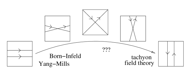
Figure 1. Intersecting D-branes: For a small intersection angle, the Non-Abelian Yang-Mills action is a valid field theory description. The Non-Abelian Born-Infeld action is more accurate but in principle also valid only for a small intersection angle. While a field theory description at large angle is not known, tachyon field theory models have been proposed for the brane-antibrane system.

As a preparation for later arguments, we review the worldsheet analysis of branes at angles in section 2. We will see that for small angles there is just one tachyonic field, a fact which naturally allows for a straightforward effective field theory treatment of the tachyon condensation. In contrast, the case of large angles is much more subtle since it contains a growing number of tachyonic field, and stringy methods are required for a proper description. In section 3 we shortly review the Yang-Mills description of branes at small angles with respect to mass spectrum matching and the role of tachyon condensation. Then, we examine brane-antibrane effective field theories and generalize these to configurations where brane and antibrane intersect at small angles. This is a first step towards filling the gap between branes at small angles and the parallel brane-antibrane case. In particular, we establish an effective action for the intersecting brane-antibrane pair by gauging a well known tachyon action for the parallel brane-antibrane pair. We argue that the specific gauge symmetry of this background ensures that the field theory fluctuation spectrum is consistent with the string theory worldsheet analysis.

2. Worldsheet analysis of branes at angles

Branes at angles have been discussed from a string worldsheet perspective in a number of papers [44, 45, 46, 36, 47]. However, these discussions have focussed on special geometries and/or small angles. To prepare the stage for the following sections, we will review the worldsheet analysis of branes at angles. Although we will follow roughly the discussion in [44, 36], we use different conventions and notation in order to keep the discussion fully general and transparent at the same time.

The boundary conditions for a string connecting the two branes at angles can be written in a compact way by introducing complex coordinates $Z^{1}=X^{2}+iX^{3}$, $Z^{2}=X^{4}+iX^{5}$, $\dots$ and similarly for the worldsheet fermions. This allows us to express the rotation taking the first brane to the second one by $Z^{a}\rightarrow\exp{-i\theta_{i}}Z^{a}$. Using this notation, the boundary conditions become:

$$\partial_{\sigma}\operatorname{Re}(Z^{a})|_{\sigma=0} = 0$$ (2.1)

$$\operatorname{Im}(Z^{a})|_{\sigma=0} = 0$$ (2.2)

$$\partial_{\sigma}\operatorname{Re}[\exp(i\theta_{a})Z^{a}]|_{\sigma=\pi} = 0$$ (2.3)

$$\operatorname{Im}[\exp(i\theta_{a})Z^{a}]|_{\sigma=\pi} = 0$$ (2.4)

for the complex bosonic field. For the following considerations, it is convenient to measure angles in units of $\pi$. If we introduce the quantities $\alpha_{a}\equiv\theta_{a}/\pi$, the classical solutions to the string equations of motion with the above boundary conditions have the following mode expansion

$$Z^{a}(z,\overline{z}) =i\left(\frac{\alpha^{\prime}}{2}\right)\sum_{n\in\mathbb{Z}}\left\{\frac{x^{a}_{n-\alpha_{a}}}{(n-\alpha_{a})z^{n-\alpha_{a}}}+\frac{x^{a\dagger}_{n+\alpha_{a}}}{(n+\alpha_{a})\overline{z}^{n+\alpha_{a}}}\right\}$$ (2.5)

$$Z^{a\dagger}(z,\overline{z}) =i\left(\frac{\alpha^{\prime}}{2}\right)\sum_{n\in\mathbb{Z}}\left\{\frac{x^{a\dagger}_{n+\alpha_{a}}}{(n+\alpha_{a})z^{n+\alpha_{a}}}+\frac{x^{a}_{n-\alpha_{a}}}{(n-\alpha_{a})\overline{z}^{n-\alpha_{a}}}\right\},$$ (2.6)

where $z=e^{i\sigma+\tau}$. Due to the complex nature of $Z$ we do not have $x^{a\dagger}_{m-\alpha_{a}}=x^{a}_{-m+\alpha}$. From canonical quantization, we get the following commutator relations

$$[x^{a\dagger}_{-m+\alpha_{a}},x^{b}_{n-\alpha_{b}}]=(-m+\alpha_{a})\delta_{ab}\delta_{mn}.$$ (2.7)

From worldsheet supersymmetry, it follows that the complexified worldsheet fermions have the same moding as the worldsheet bosons (Ramond fermions) or an additional shift by $1/2$ (Neveu-Schwarz fermions). In the following discussion, we will focus on the NS sector only because this is where tachyonic modes appear. The mode expansion becomes

$$\Psi^{a}(z)=\sum_{r\in\mathbb{Z}+\frac{1}{2}}\frac{{\psi^{a}_{r-\alpha_{a}}}}{z^{r-\frac{1}{2}-\alpha_{a}}},\qquad\Psi^{a\dagger}(z)=\sum_{s\in\mathbb{Z}+\frac{1}{2}}\frac{\psi^{a\dagger}_{s+\alpha_{a}}}{z^{s+\frac{1}{2}+\alpha_{a}}},$$ (2.8)

where the standard doubling trick has been used to extend the parameter range of the fermions to $\sigma\in[0,2\pi)$. The canonical anti-commutation relations are given by

$$\{\psi^{a\dagger}_{-r+\alpha_{a}},\psi^{b}_{s-\alpha_{b}}\}=\delta_{ab}\delta_{rs}.$$ (2.9)

The Virasoro generator $L_{0}$ is given by

$$L_{0}=\sum_{a}\left\{\sum_{m\in\mathbb{Z}}:x^{a\dagger}_{-m+\alpha_{a}}x^{a}_{m-\alpha_{a}}:+\sum_{r\in\mathbb{Z}+\frac{1}{2}}(r-\alpha):\psi^{a\dagger}_{-r+\alpha}\psi^{a}_{r-\alpha}:\right\}+\varepsilon_{0},$$ (2.10)

with a zero point energy $\varepsilon_{0}$ which can be computed from $\zeta$-function regularization of the infinite sums which arise in the process of normal ordering $L_{0}$. The exact meaning of normal ordering depends on the definition of the vacuum state. Note that the classification of mode operators in terms of creation and annihilation operators is essentially arbitrary. However, shifting an operator from “creators” to “annihilators” has an effect on the normal ordering constant such that the mass spectrum of the theory is unaffected. We will return to this issue when we discuss negative angles, $\alpha_{a}<0$. For positive angles, $\alpha_{a}>0$, it is appropriate to define the vacuum state by the properties

$$x^{a}_{m-\alpha_{a}}|0\rangle =0,\quad m\geq 1$$ (2.11)

$$x^{a\dagger}_{-m+\alpha_{a}}|0\rangle =0,\quad m\leq 0$$ (2.12)

$$\psi^{a}_{r-\alpha_{a}}|0\rangle =0,\quad r\geq 1/2$$ (2.13)

$$\psi^{a\dagger}_{-r+\alpha_{a}}|0\rangle =0,\quad r\leq-1/2.$$ (2.14)

With respect to this definition, the normal ordering constant $\varepsilon_{0}$ can be computed by a zeta function regularization procedure. The contribution due to the $a$’th complex worldsheet fields is given by (here, we are suppressing the superscript $a$ in the worldsheet fields):

$$\varepsilon_{0}^{(a)} =\sum_{m=-\infty}^{0}[x^{\dagger}_{-m+\alpha},x_{m-\alpha}]+\sum_{r=-\infty}^{-1/2}(r-\alpha)\{\psi^{\dagger}_{-r+\alpha},\psi_{r-\alpha}\}$$

$$=\sum_{m=-\infty}^{0}(-m+\alpha)+\sum_{m=-\infty}^{-1/2}(r-\alpha)$$

$$=\sum_{m=0}^{\infty}(m+\alpha)-\sum_{m=0}^{+\infty}(m+\frac{1}{2}+\alpha)$$

$$=\zeta(-1,\alpha)-\zeta(-1,1/2+\alpha)$$ (2.15)

where $\zeta$ denotes the generalized or Hurwitz zeta function which is defined by

$$\zeta(s,a)=\sum_{k=0}^{\infty}\frac{1}{(k+a)^{s}}.$$ (2.16)

The Hurwitz zeta function reduces to the ordinary (Riemann) zeta function for $a=0$. It has a well-defined analytical continuation to $s=-1$. To complete the computation of the zero point energy, we use a well-known property of the Hurwitz zeta function, which is given by:

$$\zeta(-1,\alpha)=-\frac{1}{12}+\frac{1}{2}\alpha-\frac{1}{2}\alpha^{2}$$ (2.17)

¿From this, it follows that the contribution from the $a$’th complex fields becomes

$$\varepsilon_{0}^{(a)}=-\frac{1}{8}+\frac{1}{2}\alpha_{a}.$$ (2.18)

In the computation of the total zero point energy, one has to take into account the Fadeev-Popov ghosts. As usual, their contribution cancels the contribution of two components of the worldsheet fields. There remain eight real dimensions, which add up to a value

$$\varepsilon_{0}=-\frac{1}{2}+\frac{1}{2}\sum_{a=1}^{4}\alpha_{a}.$$ (2.19)

Before we move on to determining the low-energy mass spectrum of branes at angles, we consider negative angles, $\alpha_{a}<0$. In this case, it turns out that it is most convenient to work with a slightly different definition of the vacuum state, namely:

$$x^{a}_{m-\alpha_{a}}|0\rangle =0,\quad m\geq 0$$ (2.20)

$$x^{a\dagger}_{-m+\alpha_{a}}|0\rangle =0,\quad m\leq-1$$ (2.21)

$$\psi^{a}_{r-\alpha_{a}}|0\rangle =0,\quad r\geq 1/2$$ (2.22)

$$\psi^{a\dagger}_{-r+\alpha_{a}}|0\rangle =0,\quad r\leq-1/2.$$ (2.23)

This definition differs from the one we used for positive angles in that $x^{a}_{-\alpha_{a}}$ is an annihilation operator while $x^{a\dagger}_{\alpha_{a}}$ is a creation operator. As a consequence of this shift, the zero point energy picks up an additional term of the form $-\alpha_{a}$. Then, the total zero point energy can be written in unified way

$$\varepsilon_{0}=-\frac{1}{2}+\frac{1}{2}\sum_{a=1}^{4}\left|\alpha_{a}\right|,$$ (2.24)

which is valid for both positive and negative angles. The vacuum state itself is removed by a generalization of the GSO-projection [45]. Any physical state has to contain at least one fermionic creation operator.

2.1. D-branes at one angle

As a simple example, we consider branes at one angle. These could be intersecting D-strings or more generally a pair of Dp-branes which intersect on a (p-1)-dimensional hyperplane. The latter configurations are distinguished only by the number of additional (and mutually perpendicular) Dirichlet directions. These directions do not affect the mass spectrum. Thus, all such configurations can be treated along the lines of the preceding discussion by setting all angles but one to zero. The zero point energy is then given by

$$\varepsilon_{0}=-\frac{1}{2}+\frac{1}{2}\left|\alpha\right|$$ (2.25)

where $\alpha\equiv\alpha_{1}$ is defined by the single non-vanishing angle. For small positive $\alpha$, the lowest mass state is

$$\psi^{\dagger}_{-1/2+\alpha}|0\rangle$$ (2.26)

whose mass is given by [cf. the expression (2.10) for $L_{0}$]:

$$\alpha^{\prime}m^{2}=\varepsilon_{0}+\left(\frac{1}{2}-\alpha\right)=-\frac{\alpha}{2}.$$ (2.27)

There is a tower of evenly spaced states, $(x_{-\alpha})^{n}\psi^{\dagger}_{-1/2+\alpha}|0\rangle$, with masses $\alpha^{\prime}m^{2}=(-1/2+n)\alpha$, which builds upon the lowest mass state. On the other hand, for small negative $\alpha$, there is a tower of states, $(x^{\dagger}_{\alpha})^{n}\psi_{-1/2-\alpha}$, with masses $\alpha^{\prime}m^{2}=(-1/2+n)(-\alpha)$. Both cases can be treated in a unified way by writing

$$m^{2}=\left(-\frac{1}{2}+n\right)\left|\frac{\theta}{\pi\alpha^{\prime}}\right|,\qquad n=0,1,2,\dots$$ (2.28)

for the lowest mass states, where $\theta$ is the intersection angle. This part of the mass spectrum is reproduced to order $\theta$ by the spectrum of fluctuations around an intersecting brane background in Non-Abelian Yang-Mills theory with scalar fields [1]. The T-dual configuration which has first been discussed in [36] is pure Non-Abelian Yang-Mills theory around a background with non-zero constant flux. The spectrum (2.28) has also been used to check $F^{4}$- and higher order terms in the Non-Abelian Born-Infeld action [1, 41].

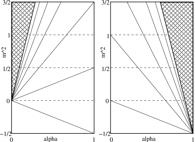
Figure 2. These plots show part of the NS spectrum on intersecting branes. The states on the left constitute the tower of lowest mass states for configurations which are close to parallel branes. These become momentum states at vanishing intersection angle ($\alpha=0$). The states on the right become the (tachyonic) lowest mass states for configurations which are close to the brane-antibrane pair. They become momentum states for $\alpha=1$.

However, it is important to note that this spectrum does no longer represent the lowest mass excited states when one takes $\theta$ to be large. To see what exactly happens to the low-lying mass spectrum when the intersection angle flows from $\theta=0$ (parallel brane-brane system) to $\theta=\pi$ (parallel brane-antibrane system), note that the states created by $x^{\dagger}_{-\alpha}$ become increasingly heavy while states created by $x_{-1+\alpha}$ become increasingly light. At $\alpha=1/2$, which corresponds to perpendicular branes, the two families of excitations exchange roles. Finally, when one is approaching the brane-antibrane system, the low-lying excitations are $\psi^{\dagger}_{-1/2+\alpha}(x_{-1+\alpha})^{n}|0\rangle$ and their mass spectrum is given by

$$\alpha^{\prime}m^{2}=\varepsilon_{0}+\left(\frac{1}{2}-\alpha\right)+n(1-\alpha),\quad n=0,1,2,\dots$$ (2.29)

Using the relation (2.25) this becomes:

$$m^{2}=-\frac{1}{2\alpha^{\prime}}+\frac{\phi}{2\pi\alpha^{\prime}}(2n+1),\quad n=0,1,2,\dots$$ (2.30)

where $\phi\equiv\pi-\theta$ is the intersection angle between the brane and antibrane. In the limit of $\phi\rightarrow 0$, the mass tower collapses and the corresponding oscillators become momentum states. This is just what happens for the brane-brane case, when $\theta\rightarrow 0$. Figure 2 is a graphic representation of the low-lying spectrum on intersecting branes. Note that due to our definition of the vacuum state, $x_{-1/2+\alpha}$ is a creation operator even for $\alpha>1/2$ in contrast to the usual conventions. One could redefine the vacuum state for systems which are close to the brane-antibrane system, thereby shifting $x_{-1/2+\alpha}$ to the annihilation operators but this would again imply a modification of the normal ordering constant which ensures that the mass spectrum stays the same.

2.2. D-branes at two and three angles

As an illustration of the many-angles case, consider a pair of intersecting D2-branes (alternatively: Dp-branes intersecting on a (p-2)-dimensional hyperplane). For small positive intersection angles, the lowest-lying states are given by

$$\psi^{1\dagger}_{-1/2+\alpha_{1}}(x^{1}_{-\alpha_{1}})^{n_{1}}(x^{2}_{-\alpha_{2}})^{n_{2}}|0\rangle \quad\alpha^{\prime}m^{2}=(n_{1}-1/2)\alpha_{1}+(n_{2}+1/2)\alpha_{2}$$

$$\psi^{2\dagger}_{-1/2+\alpha_{2}}(x^{1}_{-\alpha_{1}})^{n_{1}}(x^{2}_{-\alpha_{2}})^{n_{2}}|0\rangle \quad\alpha^{\prime}m^{2}=(n_{1}+1/2)\alpha_{1}+(n_{2}-1/2)\alpha_{2}$$

$$\psi^{1}_{-1/2-\alpha_{1}}(x^{1}_{-\alpha_{1}})^{n_{1}}(x^{2}_{-\alpha_{2}})^{n_{2}}|0\rangle \quad\alpha^{\prime}m^{2}=(n_{1}+3/2)\alpha_{1}+(n_{2}+1/2)\alpha_{2}$$ (2.31)

$$\psi^{2}_{-1/2-\alpha_{2}}(x^{1}_{-\alpha_{1}})^{n_{1}}(x^{2}_{-\alpha_{2}})^{n_{2}}|0\rangle \quad\alpha^{\prime}m^{2}=(n_{1}+1/2)\alpha_{1}+(n_{2}+3/2)\alpha_{2}$$

$$\psi^{\mu}_{-1/2}(x^{1}_{-\alpha_{1}})^{n_{1}}(x^{2}_{-\alpha_{2}})^{n_{2}}|0\rangle \quad\alpha^{\prime}m^{2}=(n_{1}+1/2)\alpha_{1}+(n_{2}+1/2)\alpha_{2}$$

where $\psi^{\mu}$ is a fermionic creation operator in a dimension where both branes are point-like. The masses are computed by adding the appropriate contributions from the creation operators to the zero-point energy $\varepsilon_{0}$. Generically, the lowest mass state is tachyonic with two evenly spaced towers of low-energy excited states on top of it. The towers’ spacing is $\alpha_{1}$ and $\alpha_{2}$ respectively. There is one special configuration where the lowest mass state becomes massless, namely when $\theta_{1}=\theta_{2}$. This is a well-known supersymmetric brane configuration. Contrastingly, if the angles have opposite sign (say $\alpha_{1}>0$, $\alpha_{2}<0$), the lowest-lying states and their masses are given by

$$\psi^{1\dagger}_{-1/2+\alpha_{1}}(x^{1}_{-\alpha_{1}})^{n_{1}}(x^{2\dagger}_{\alpha_{2}})^{n_{2}}|0\rangle \quad\alpha^{\prime}m^{2}=(n_{1}-1/2)\alpha_{1}-(n_{2}+1/2)\alpha_{2}$$

$$\psi^{2}_{-1/2-\alpha_{2}}(x^{1}_{-\alpha_{1}})^{n_{1}}(x^{2\dagger}_{\alpha_{2}})^{n_{2}}|0\rangle \quad\alpha^{\prime}m^{2}=(n_{1}+1/2)\alpha_{1}-(n_{2}-1/2)\alpha_{2}$$

$$\psi^{1}_{-1/2-\alpha_{1}}(x^{1}_{-\alpha_{1}})^{n_{1}}(x^{2\dagger}_{-\alpha_{2}})^{n_{2}}|0\rangle \quad\alpha^{\prime}m^{2}=(n_{1}+3/2)\alpha_{1}-(n_{2}+1/2)\alpha_{2}$$ (2.32)

$$\psi^{2\dagger}_{-1/2+\alpha_{2}}(x^{1}_{-\alpha_{1}})^{n_{1}}(x^{2\dagger}_{-\alpha_{2}})^{n_{2}}|0\rangle \quad\alpha^{\prime}m^{2}=(n_{1}+1/2)\alpha_{1}-(n_{2}+3/2)\alpha_{2}$$

$$\psi^{\mu}_{-1/2}(x^{1}_{-\alpha_{1}})^{n_{1}}(x^{2\dagger}_{-\alpha_{2}})^{n_{2}}|0\rangle \quad\alpha^{\prime}m^{2}=(n_{1}+1/2)\alpha_{1}-(n_{2}+1/2)\alpha_{2}$$

and the spectrum becomes tachyon-free for $\alpha_{1}=-\alpha_{2}$. For branes at two small angles $\theta_{1}$ and $\theta_{2}$, the lowest part of the mass spectrum can therefore be summarized by the formula (not counting degeneracies)

$$m^{2}=\left(-\frac{1}{2}+n_{1}\right)\left|\frac{\theta_{1}}{\pi\alpha^{\prime}}\right|+\left(-\frac{1}{2}+n_{2}\right)\left|\frac{\theta_{2}}{\pi\alpha^{\prime}}\right|,\quad n_{1},n_{2}=0,1,2,\dots$$ (2.33)

Contrastingly, if for positive angles we let $\theta_{2}$ approach $\pi$ while keeping $\theta_{1}$ small at the same time we get to a configuration where a brane and an antibrane intersect at small angles $\theta\equiv\theta_{1}$ and $\phi\equiv\pi-\theta_{2}$. The lowest mass states are now given by

$$\psi^{2\dagger}_{-1/2+\alpha_{2}}(x_{-\alpha_{1}}^{1})^{n_{1}}(x^{2}_{-1+\alpha_{2}})^{n_{2}}|0\rangle$$ (2.34)

and the corresponding mass spectrum is given by

$$m^{2}=-\frac{1}{2\alpha^{\prime}}+\frac{\theta}{\pi\alpha^{\prime}}(2n_{1}+1)+\frac{\phi}{\pi\alpha^{\prime}}(2n_{2}+1),\quad n_{1},n_{2}=0,1,2,\dots$$ (2.35)

If we let both intersection angles approach their maximum value, we once more end up with a brane-brane configuration because this operation reverses the relative brane orientation twice. Consistently, the mass spectrum is the same as in (2.33) upon substituting $\theta_{1}\rightarrow\pi-\theta_{1},\theta_{2}\rightarrow\pi-\theta_{2}$.

The discussion could now be easily continued also to the case of D-branes at three angles. Here the tachyon-free, supersymmetric configuration is obtained, if $\theta_{1}+\theta_{2}+\theta_{3}=\pi$. There are four scalar fields living at each intersection that could become tachyonic. The stability conditions are somewhat more complicated compared to the case of two D-branes. In particular it turns out there exist an extended region of stability, namely the angle parameter space can be represented as a tetrahedron [7, 48]. On the walls of the tetrahedron one supersymmetry is preserved. For small deviations outside the tetrahedron one of the four scalar fields becomes tachyonic. So outside the tetrahedron the tachyon condensation will takes place, and there will be a decay to another system. Going to larger angles outside the tetrahedron one again enters the region of getting more and more tachyonic fields. However inside the tetrahedron there are no tachyons at all, and the system is stable despite of not being supersymmetric.

3. Branes at small angles

Before we consider field theory descriptions of branes at large angles, we would like to review some results from the familiar Yang-Mills action for branes at small angles such as its fluctuation mass spectrum and the role of tachyon condensation. The Yang-Mills description of low energy brane dynamics provides an explicit realization of brane recombination processes and local brane-antibrane annihilation. This has been shown recently in a paper by Hashimoto and Nagaoka [1]. They considered a Yang-Mills background corresponding to intersecting D-Strings in a non-compact geometry. An analysis of the Yang-Mills fluctuation fields shows that the condensation of the tachyonic mode can be related to brane-recombination by a local gauge transformation of the brane-coordinates. The following paragraph will largely follow their discussion of the fluctuation analysis, filling in some further details. In particular, we compute the tachyon potential in the Yang-Mills framework and discuss its relevance for brane recombination processes. We also find an infinite family of moduli in the fluctuation spectrum of the intersecting brane solution and show that they generate gauge transformations of the background fields.

The Yang-Mills action for the problem is the dimensionally reduced pure Yang-Mills action

$$S=-\frac{1}{2}\int d^{2}x\operatorname{Tr}\left(F_{\mu\nu}F^{\mu\nu}+2D_{\mu}\Phi D^{\mu}\Phi\right)$$ (3.1)

where we choose to set the coupling constant to one and omit fermions. The scalar field $\Phi$ is given by the scaled brane coordinates in the $y$-direction: $\Phi=2\pi\alpha^{\prime}Y$. The background solution corresponding to two D-Strings intersecting at an angle $\theta$ is given by

$$\Phi=qx(1/2)\tau_{3}$$ (3.2)

$$A_{\mu}=0$$ (3.3)

where q is related to the intersection angle by

$$q=\frac{1}{\pi\alpha^{\prime}}\tan(\theta/2).$$ (3.4)

Expanding the action (3.1) around the background (3.2) leads to the quadratic Lagrangian for the fluctuation fields. The diagonal fluctuations (those which are proportional to $\mathbf{1}$ or $\tau_{3}$) commute with the background fields. Therefore they decouple from all other fluctuations and satisfy free field equations. We can neglect them in the following discussion. In order to follow the discussion in [1], one has to impose one condition on the fluctuation fields, namely $\delta A_{0}=0$. The remaining four fluctuation fields are then grouped in pairs which decouple from each other at the quadratic level. However, note that one cannot simply use gauge invariance to go to Coulomb gauge because this would at the same time modify the gauge field background. In fact, choosing a specific background generally fixes the gauge symmetry completely. K. Hashimoto, in private communication, justifies setting $\delta A_{0}=0$ by saying that the gauge transformation which is needed to do this is small when compared to the background fields and that the small modification of the gauge background could be interpreted as fluctuations in other sectors than $A_{0}$ after the gauge transformation. We rather prefer to see the spectrum one obtains by setting $\delta A_{0}=0$ as a significant part of the full spectrum, which can be investigated with relative ease. Having said this, we will from now on assume $\delta A_{0}=0$ and continue in the analysis by defining:

$$\delta A_{1}^{2}\equiv a,\qquad\delta\Phi^{1}\equiv\varphi,$$ (3.5)

$$\delta A_{1}^{1}\equiv b,\qquad\delta\Phi^{2}\equiv\psi.$$ (3.6)

Then, the quadratic Lagrangian for the fluctuation fields splits in two parts: $\mathcal{L}=\mathcal{L}_{A}+\mathcal{L}_{B}$ with

$$\mathcal{L}_{A} =\frac{1}{2}(\partial_{t}a)^{2}+\frac{1}{2}(\partial_{t}\varphi)^{2}-\frac{1}{2}(\partial_{x}\varphi)^{2}-\frac{1}{2}q^{2}x^{2}a^{2}-qa\varphi+qxa\partial_{x}\varphi,$$ (3.7)

$$\mathcal{L}_{B} =\frac{1}{2}(\partial_{t}b)^{2}+\frac{1}{2}(\partial_{t}\psi)^{2}-\frac{1}{2}(\partial_{x}\psi)^{2}-\frac{1}{2}q^{2}x^{2}b^{2}+qb\psi-qxb\partial_{x}\psi.$$ (3.8)

We can decompose the fluctuation fields into their mass eigenstates by setting

$$\begin{pmatrix}a(t,x)\\ \varphi(t,x)\end{pmatrix}=\sum_{n}\begin{pmatrix}a_{n}(x)\\ \varphi_{n}(x)\end{pmatrix}\exp(-im_{n}t)$$ (3.9)

and similarly for $(b,\psi)$. The mass spectrum is a priori continuous but it will turn out that requiring normalizablility for the wave functions (which is equivalent to demanding that the action be finite) leads to an integer index $n$. The equations of motion for the fluctuation fields $(a,\varphi)$ are

$$\begin{pmatrix}-q^{2}x^{2}+m_{n}^{2}&+qx\partial_{x}-q\\ -qx\partial_{x}-2q&\partial_{x}^{2}+m_{n}^{2}\end{pmatrix}\begin{pmatrix}a_{n}(x)\\ \varphi_{n}(x)\end{pmatrix}=0.$$ (3.10)

The equations of motion for $(b,\psi)$ can be derived from these by substituting $(a,\varphi)\leftrightarrow(b,\psi)$ because this substitution interchanges $\mathcal{L}_{A}$ and $\mathcal{L}_{B}$. Therefore we can focus on the pair $(a,\varphi)$. From the simultaneous appearance of terms involving $x\partial_{x}$ and $x^{2}$ respectively we can guess that the solution to the equations of motion will asymptotically look like a Gaussian. The corresponding localization of the fluctuation modes around $x=0$ is consistent with the string theory picture, where strings stretching from one brane to the other are naturally confined to the intersection point due to their finite tension. Setting

$$a_{n}(x)=\exp(-qx^{2}/2)p_{n}(x),\qquad\varphi_{n}(x)=\exp(-qx^{2}/2)q_{n}(x)$$ (3.11)

leads to modified equations of motion:

$$\begin{pmatrix}-q^{2}x^{2}+m_{n}^{2}&-q-q^{2}x^{2}+qx\partial_{x}\\ +q^{2}x^{2}-qx\partial_{x}-2q&m_{n}^{2}-q+q^{2}x^{2}-2qx\partial_{x}+\partial_{x}^{2}\end{pmatrix}\begin{pmatrix}p_{n}(x)\\ q_{n}(x)\end{pmatrix}=0.$$ (3.12)

If we assume that $p_{n}$ and $q_{n}$ are polynomials, this implies that the fluctuation wave functions are normalizable indeed. Polynomial solutions are possible only for discrete values of $m^{2}_{n}$. These are given by

$$m^{2}_{n}=(2n-1)q;\quad n=0,2,3,4,\dots$$ (3.13)

In addition, there are solutions for $m^{2}=0$, which were omitted in ref. [1]. The mass values (3.13) are consistent to the worldsheet analysis (2.28) up to a substitution $\tan(\theta/2)\rightarrow\theta/2$. This discrepancy reflects the fact that the Yang-Mills description is only viable for small angles. The corresponding solutions for the fluctuation wave functions are:

$$p_{n}(x) =-\sum_{j=1,3,\cdots}^{n}(-1)^{j/2}\frac{4^{j/2}}{j!}\frac{n(n-2)\cdots(n-j+2)}{2n-1}(j-1)\left(x\sqrt{q/2}\right)^{j}$$ (3.14)

$$q_{n}(x) =\sum_{j=1,3,\cdots}^{n}(-1)^{j/2}\frac{4^{j/2}}{j!}\frac{n(n-2)\cdots(n-j+2)}{2n-1}(2n-j-1)\left(x\sqrt{q/2}\right)^{j}$$ (3.15)

for $n=0,2,4,\dots$ and

$$p_{n}(x) =-\sum_{j=1,3,\cdots}^{n}(-1)^{j-1/2}\frac{4^{j-1/2}}{j!}\left(\frac{j-1}{2}\right)(n-3)\cdots(n-j+2)\left(x\sqrt{q/2}\right)^{j}$$ (3.16)

$$q_{n}(x) =\sum_{j=1,3,\cdots}^{n}(-1)^{j-1/2}\frac{4^{j-1/2}}{j!}\left(n-\frac{j+1}{2}\right)(n-3)\cdots(n-j+2)\left(x\sqrt{q/2}\right)^{j}$$ (3.17)

for $n=3,5,7,\dots$. These solutions were given by Hashimoto and Nagaoka in [1]. A curious fact is that there is no polynomial solution for $n=1$; $m^{2}=q$ although this mass level has to be included from the worldsheet perspective. The solutions for $(b,\psi)$ are obtained by

$$b_{n}(x)=\exp(-qx^{2}/2)p_{n}(x),\qquad\psi_{n}(x)=-\exp(-qx^{2}/2)q_{n}(x).$$ (3.18)

Hashimoto and Nagaoka pointed out that the geometric interpretation of the tachyonic modes is a brane recombination process. The negative mass squared means that a non-zero tachyon amplitude blows up exponentially

$$\varphi(t,x)=C(t)\varphi(x)$$ (3.19)

with

$$C(t)=\exp(\sqrt{-m^{2}}t)C(0)=\exp(\sqrt{q}t)C(0)$$ (3.20)

and similarly for $a$, $b$, and $\psi$. Now turn on the tachyonic mode of one pair, say $(a,\varphi)$ and consider the total scalar field $\Phi(x)$, including background and fluctuations, with the explicit expression for the tachyonic mode plugged in:

$$\Phi(t,x) =\Phi^{0}(x)+\varphi(t,x)\frac{1}{2}\tau^{1}$$ (3.21)

$$=\frac{1}{2}\begin{pmatrix}qx&C(t)\varphi(x)\\ C(t)\varphi(x)&-qx\end{pmatrix}$$ (3.22)

To get to a geometric interpretation, one has to gauge transform $\Phi(x)$ such that it becomes diagonal. Under a gauge transformation $U$, $\Phi$ transforms as $\Phi\rightarrow U\Phi U^{-1}$ (remember that $\Phi$ is derived from the gauge field $A_{2}$ by dimensional reduction), so that we are faced with an ordinary eigenvalue problem which is easily solved. The diagonalized field is given by

$$\Phi(t,x)=\frac{1}{2}\begin{pmatrix}\sqrt{q^{2}x^{2}+C(t)^{2}\varphi(x)^{2}}&0\\ 0&-\sqrt{q^{2}x^{2}+C(t)^{2}\varphi(x)^{2}}\end{pmatrix}.$$ (3.23)

The corresponding brane coordinates are recovered by setting $Y_{i}=2\pi\alpha^{\prime}\Phi_{ii}$. Using the explicit expression for the tachyonic mode [cf. (3.11) and (3.15)], they are given by

$$Y_{1,2}=\pm\pi\alpha^{\prime}\sqrt{q^{2}x^{2}+C(t)^{2}exp(-qx^{2}/2)}$$ (3.24)

This clearly describes a recombination process, which is illustrated in figure 3.

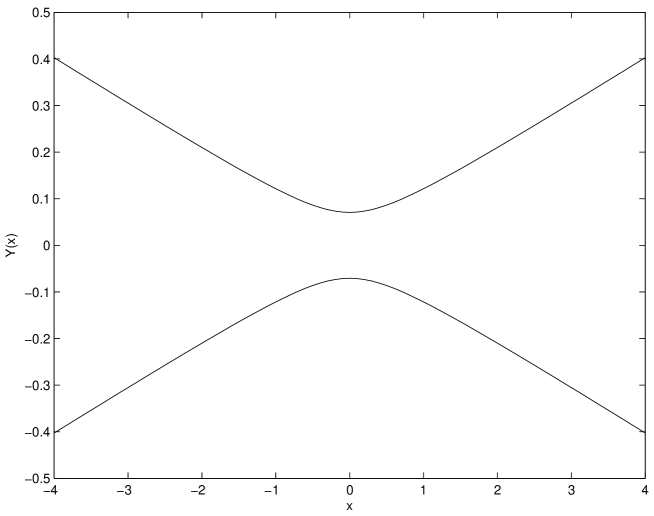
Figure 3. Recombination of intersecting D-Strings via tachyon condensation. For this plot, we have evaluated equation (3.24) with parameters $q=1/10$ and $C^{2}=1/200$. $\pi\alpha^{\prime}$ has been set to unity.

3.1. Moduli in intersecting branes

As we mentioned before, there is an infinite family of moduli in addition to the tachyonic modes and the tower of massive states that were discussed in the last paragraph. These were overlooked by Hashimoto and Nagaoka. With the same conventions as used in the last section, setting $m^{2}=0$ gives the following equations of motion for the polynomial factors $(p,q)$ of the $(a,\phi)$ pair of fluctuation fields:

$$\begin{pmatrix}-q^{2}x^{2}&-q-q^{2}x^{2}+qx\partial_{x}\\ +q^{2}x^{2}-qx\partial_{x}-2q&-q+q^{2}x^{2}-2qx\partial_{x}+\partial_{x}^{2}\end{pmatrix}\begin{pmatrix}p_{n}(x)\\ q_{n}(x)\end{pmatrix}=0.$$ (3.25)

The dependence on $q$ can be eliminated by rescaling $x\rightarrow\sqrt{q/2}\ x$. Then the equations take the following form

$$\begin{pmatrix}-2x^{2}&-1-2x^{2}+x\partial_{x}\\ 2x^{2}-x\partial_{x}-2&-1+2x^{2}-2x\partial_{x}+\frac{1}{2}\partial_{x}^{2}\end{pmatrix}\begin{pmatrix}p_{n}(x)\\ q_{n}(x)\end{pmatrix}=0.$$ (3.26)

To solve these equations, we define new polynomials $f$, $g$ by

$$f(x) =\frac{1}{2}(p(x)+q(x))$$ (3.27)

$$g(x) =\frac{1}{2}(p(x)-q(x))$$ (3.28)

leading to equations of motion:

$$\begin{pmatrix}-4x^{2}-1+x\partial_{x}&1-x\partial_{x}\\ -8x^{2}-\partial_{x}^{2}+6x\partial_{x}+6&-2x\partial_{x}+2+\partial_{x}^{2}\end{pmatrix}\begin{pmatrix}f(x)\\ g(x)\end{pmatrix}=0.$$ (3.29)

If one defines

$$f(x)=\sum_{j=0}^{n}f_{j}x^{j};\qquad g(x)=\sum_{j=0}^{n^{\prime}}g_{j}x^{j}$$ (3.30)

with $g_{n}\equiv 1$, one gets equations for the coefficients:

$$j\geq 2: \begin{cases}-(j-1)g_{j}+(j-1)f_{j}-4f_{j-2}=0\\ (j+2)(j+1)g_{j+2}-2(j-1)g_{j}\\ \quad-(j+2)(j+1)f_{j+2}+6(j+1)f_{j}-8f_{j-2}=0\end{cases}$$ (3.31)

$$j=1: \quad g_{3}-f_{3}+2f_{1}=0$$ (3.32)

$$j=0: \begin{cases}g_{0}-f_{0}=0\\ g_{2}-f_{2}+4f_{0}=0\end{cases}$$ (3.33)

While setting $j=n+2$ shows that $f_{n}=0$, setting $j=n$ leads to $f_{n-2}=-(n-1)/4$. Now setting $j=n-2$ gives two equations for the two variables $f_{n-2}$ and $g_{n-4}$. It turns out that these are not linearly independent, so one can freely choose one of the variables. It is convenient to require $f_{n-4}=0$, which means that we must have $f_{n-2}=g_{n-2}$. Then all other component equations can be satisfied by setting $f_{j}=g_{j}=0$ for $j\leq n-2$. Because we chose to set $f_{n-4}=0$, the above solution is not unique but note that giving any other value to $f_{n-4}$ is equivalent to adding a solution of the form $\{g_{n-2}=1$, $g_{j}=0$ for $j>(n-1)\}$. Altogether we have solutions

$$\begin{pmatrix}f(x)\\ g(x)\end{pmatrix}=\begin{pmatrix}-\frac{n-1}{4}x^{n-2}\\ x^{n}-\frac{n-1}{4}x^{n-2}\end{pmatrix}$$ (3.34)

for $n=2,3,\dots$ and, in addition, the solution $(f,g)=(0,x)$. The most general solution is given by a linear combination of these. In terms of the original variables, the solutions are given by

$$\begin{array}[]{ccl}a(x)&=&\exp\left(-qx^{2}/2\right)(qx^{n}-(n-1)x^{n-2}),\\ \varphi(x)&=&-\exp\left(-qx^{2}/2\right)qx^{n}\end{array}$$ (3.35)

for $n=2,3,\dots$ where we absorbed a global ($n$-dependent) factor by rescaling. The additional solution takes the form

$$\begin{array}[]{ccl}a(x)&=&\exp\left(-qx^{2}/2\right)x,\\ \varphi(x)&=&-\exp\left(-qx^{2}/2\right)x.\end{array}$$ (3.36)

As before, the solutions for $(b,\psi)$ can be obtained by substituting $(a,\phi)\leftrightarrow(b,-\psi)$. To see the geometrical interpretation of the zero modes, we refer to the diagonal form (3.23) of the scalar field $\Phi$, with fluctuations included. The worldlines of the D-strings are given by

$$Y(t,x)=\pm 2\pi\alpha^{\prime}\frac{1}{2}\sqrt{q^{2}x^{2}+C(t)\varphi(x)^{2}}.$$ (3.37)

The zero mass modes do not evolve in time so that $C$ is simply a constant. For $\varphi(x)$ we can take any superposition of the massless solutions (3.35) and (3.36), so that the most general case is given by $\varphi(x)=x\exp(-qx^{2}/2)P(x)$ with $P(x)$ an arbitrary polynomial. This means that we can arbitrarily deform the worldlines of the D-strings in the vicinity of the intersection point as long as the deformations remain small (away from the intersection point, the fluctuations are damped by the exponential factor). There is one restriction to possible deformations, namely that because $\varphi(x)$ goes to zero like $x$ or faster when $x$ approaches zero, the worldlines will always intersect. Intuitively, deformations of the D-string worldlines should not be massless because the D-strings are wrapped around a torus (possibly with infinite radius) and they have a finite tension which should work against any wriggles in the worldlines. But note that the tension is not the only contribution to the energy density because $\varphi$ can only be turned on in conjunction with $a$, which also contributes to the $D_{\mu}\Phi D^{\mu}\Phi$ term. Since massless fluctuation modes by construction do not change the energy of a background configuration, we have to assume that all contributions to the energy coming from fluctuation modes cancel in the end. The question remains what the meaning of the massless modes is, in particular because they do not appear in the string theory spectrum. The logical answer to this is that the massless modes are remnants of the original gauge symmetry. Turning on their amplitude is equivalent to gauge transforming the background fields. To see this, we consider a gauge transformation of the form

$$A_{1}^{0} \rightarrow\tilde{A}^{0}_{1}\equiv UA_{1}^{0}U^{-1}-(\partial_{x}U)U^{-1}$$

$$\Phi^{0} \rightarrow\tilde{\Phi^{0}}\equiv U\Phi^{0}U^{-1}$$ (3.38)

where

$$U(x) =\exp(i\Lambda(x))$$

$$\Lambda(x) =\exp(-qx^{2}/2)x^{n-1}(\tau_{2}/2).$$ (3.39)

If we consider infinitesimal gauge transformations, we can neglect quadratic and higher terms in $\Lambda$. By plugging in the explicit expressions (3.2) for the intersecting brane background into equations (3.38) and expanding to linear order in $\Lambda$ we find that the transformed background fields are given by

$$\tilde{A}^{0}_{1} =A^{0}_{1}+\exp(-qx^{2}/2)(qx^{n}-(n-1)x^{n-2})(\tau_{2}/2)$$ (3.40)

$$\tilde{\Phi}^{0} =\Phi^{0}-\exp(-qx^{2}/2)qx^{n}(\tau_{1}/2).$$ (3.41)

As we expected, these expressions are the sum of the untransformed background fields and fluctuation fields of the form (3.35). In other words, the massless fluctuation modes generate gauge transformations of the background fields. In fact, choosing a particular gauge background breaks the $U(2)$-gauge symmetry of the Yang-Mills action spontaneously and the massless fluctuations are components of the corresponding Goldstone scalar. Since gauge transformations relate physically equivalent configurations, this Goldstone scalar describes a redundancy of the formalism rather than a physical degree of freedom. Thus, we resolve the apparent contradiction to the string worldsheet analysis.

4. Branes at large angles

As has been pointed out, non-Abelian Yang-Mills theory fails to describe intersecting branes at large angles. However, by increasing one intersection angle continuously (keeping all other angles at zero) one eventually arrives at a coincident brane-antibrane pair. This is a configuration which has been thoroughly investigated from the tachyon field theory perspective and it seems promising to generalize existing tachyon actions to include small intersection angles between the brane and antibrane.

Much of the work on the brane-antibrane system has been inspired by Sen’s conjectures on tachyon condensation [49, 50, 51, 52]. With the tachyon rolling down towards its potential’s minimum, standard first quantized string theory fails because it is only defined around the perturbative vacuum. Therefore one has to resort to string field theory methods. For some time the focus had been on numerical studies using Witten’s cubic string field theory but more recently Boundary String Field Theory (BSFT) has produced a number of exact results on tachyon condensation. One particular success of BSFT has been the derivation of an effective tachyon action for a non-BPS brane.

$$S=-\int d^{p+1}xe^{-T^{2}/4}\left(1+\frac{1}{2}\partial_{\mu}T\partial^{\mu}T\right)$$ (4.1)

This action had originally been proposed as a toy model for tachyon condensation [53] and was subsequently shown to be an exact two-derivative truncation of the full BSFT [54]. We are not keeping track of overall numerical factors of the action here and $\alpha^{\prime}$ has been set to unity.

A non-BPS brane is a “wrong p” Dp-brane meaning odd dimension D-branes in type IIA theory and even dimension D-branes in type IIB theory. It breaks supersymmetry completely and is expected to decay to a stable BPS D(p-1)-brane via tachyon condensation. We will use the non-BPS brane tachyon action as a starting point for establishing an effective action for branes and antibranes intersecting at small angles. There will be two major modifications to the action (4.1). First, it has to be lifted to the brane-antibrane case, which is in fact closely related to the non-BPS brane via brane descent relations. Next, we need to introduce gauge fields to the action because a non-zero magnetic flux is related to non-zero intersection angles via T-duality. In the BSFT approach, it is notoriously difficult to include gauge fields from the beginning because the corresponding boundary terms introduce non-trivial interactions in the BSFT action. Thus, the theory is no longer exactly solvable and one has to make do with perturbational computations. However, one can sidestep these complications by manufacturing a tachyon action “by hand”. We will explain the sort of hand-waving arguments which are needed in such a construction and “derive” a simple gauged $D\overline{D}$-action.

4.1. A simple gauged $D\overline{D}$-action

In the brane-antibrane system, the tachyonic modes come from strings which connect brane and anti-brane. The fact that there are two possible orientations for such strings leads to a degeneracy of the string theory spectrum. This can be dealt with by making the tachyon field in (4.1) complex. Thus, a natural generalization of the non-BPS-brane action would be:

$$S=-\int d^{p+1}xe^{-\overline{T}T/4}\left(1+\frac{1}{2}\partial_{\mu}\overline{T}\partial^{\mu}T\right).$$ (4.2)

This action has global $U(1)$-symmetry. To gauge the symmetry in a standard way, the derivatives have to be covariantized, $\partial_{\mu}\rightarrow D_{\mu}$ where

$$D_{\mu}=\partial_{\mu}-iA_{\mu}.$$ (4.3)

What is the meaning of the gauge field $A_{\mu}$, which we just introduced? Clearly, it should be related to some abelian subgroup of the original $U(2)$-symmetry of a two-brane system. The Chan-Paton representation of the complex tachyon state is given by

$$\begin{pmatrix}0&\overline{T}\\ T&0\end{pmatrix}.$$ (4.4)

This transforms under the adjoint representation of $U(2)$. Now consider a special family of $U(2)$ transformations,

$$\begin{pmatrix}0&\overline{T}\\ T&0\end{pmatrix}\rightarrow\begin{pmatrix}0&\rho_{1}^{*}\rho_{2}\overline{T}\\ \rho_{2}^{*}\rho_{1}T&0\end{pmatrix}=\begin{pmatrix}\rho_{1}^{*}&0\\ 0&\rho_{2}^{*}\end{pmatrix}\begin{pmatrix}0&\overline{T}\\ T&0\end{pmatrix}\begin{pmatrix}\rho_{1}&0\\ 0&\rho_{2}\end{pmatrix}$$ (4.5)

where $\rho_{1}^{*}\rho_{1}=\rho_{2}^{*}\rho_{2}=1$. Clearly, the tachyon state is neutral under the combination $\rho_{1}=\rho_{2}$ while it is charged under $\rho_{1}=\rho_{2}^{*}$. Since $\rho_{1}$ and $\rho_{2}$ correspond to abelian gauge transformations on the first and second brane respectively, the correct form for the covariant derivative in (4.3) is given by $A_{\mu}=A_{\mu}^{(1)}-A_{\mu}^{(2)}$ where $A_{\mu}^{(i)}$ are the abelian gauge fields on the individual branes. Next, we have to include gauge invariant kinetic terms for the gauge field in the tachyon action. The simplest option clearly is:

$$S=-\int d^{p+1}xe^{-\overline{T}T/4}\left(1+\frac{1}{4}F_{\mu\nu}F^{\mu\nu}+\frac{1}{2}D_{\mu}\overline{T}D^{\mu}T\right).$$ (4.6)

Introducing kinetic terms in this way also ensures that for $T\equiv 0$ the theory reduces to standard gauge theory of the unbroken Abelian symmetry. Of course, this is by far not the only possibility for including gauge kinetic terms. We will shortly discuss two more options at the end of this section. For now, we will stick to the simple action given above. Being interested in low-energy physics near the perturbative vacuum at $T=0$, we can make a further approximation. After reinserting factors of $\alpha^{\prime}$, the action becomes

$$S=S_{0}-\int d^{p+1}\left(\frac{1}{4}F^{\mu\nu}F_{\mu\nu}+\frac{1}{2}D_{\mu}\overline{T}D^{\mu}T-\frac{1}{4\alpha^{\prime}}\left|T\right|^{2}\right)$$ (4.7)

up to zeroth order in $\alpha^{\prime}$ ($\cong$ low-energy) and second order in the tachyon field ($\cong$ near the perturbative vacuum). Note that since we are not keeping track of overall numerical factors, the order in $\alpha^{\prime}$ is only relative. ¿From this, the action for intersecting brane-antibrane systems (i.e. intersecting branes at large angle) is derived by applying T-duality in the form of dimensional reduction. The part of the action containing the tachyon field becomes:

$$S=-\int d^{p^{\prime}+1}\left(\partial_{\mu}\overline{T}\partial^{\mu}T+\left(\sum_{I}\frac{\Delta Y^{I}(x)\Delta Y^{I}(x)}{(2\pi\alpha^{\prime})^{2}}-\frac{1}{2\alpha^{\prime}}\right)\left|T\right|^{2}\right)$$ (4.8)

$$\Delta Y^{I}\equiv Y^{(1)I}-Y^{(2)I}$$ (4.9)

where $Y^{(i)I}$ are the transverse coordinates of brane ($i=1$) and antibrane ($i=2$) and we have set the gauge field on the remaining brane dimensions to zero. Now we see that everything fits together neatly. For parallel brane and antibrane with non-zero separation, the term with the $\Delta Y$’s simply reproduces the tension from stretched strings which reduces the negative mass squared of the tachyon. For intersecting branes, the same term leads to a localization of the tachyon modes on the intersection manifold and a mass spectrum with towers of evenly spaced states. For simplicity, we consider the string-antistring case. Then, the background corresponding to an intersection angle $\phi$ is given by $Y^{(1,2)}=\pm\tan(\phi/2)x$ and therefore $\Delta Y(x)=2\tan(\phi/2)x$. The action (4.8) is by virtue of its “derivation” essentially a small angle approximation because $\tan(\phi/2)$ is proportional to the field strength amplitude in (4.7) and higher order terms in the field strength would correspond to corrections which are higher order in $\alpha^{\prime}$. Thus, within the range of validity of (4.8) we can approximate by setting $\tan(\phi/2)\approx\phi/2$. The action becomes

$$S=\int dtdx\left[\partial_{t}\overline{T}\partial_{t}T-\overline{T}\left(-\partial_{x}^{2}+\left(\frac{\phi}{2\pi\alpha^{\prime}}\right)^{2}x^{2}-\frac{1}{2\alpha^{\prime}}\right)T\right].$$ (4.10)

This involves a harmonic oscillator potential. Thus, the tachyon fluctuation modes are localized at the intersection point at $x=0$. The mass spectrum of the tachyon field fluctuations which one computes from the above action is given by

$$m^{2}=-\frac{1}{2\alpha^{\prime}}+\frac{\phi}{2\pi\alpha^{\prime}}(2n+1),\quad n=0,1,2,\dots$$ (4.11)

Surprisingly, this coincides exactly with the worldsheet analysis which was given in section 2 [cf. (2.30)]. This observation stays valid for higher dimensional branes and multiple intersection angles. The exact matching of mass spectra should be seen as a strong argument in favor of the empirical action (4.7).

In [1], Hashimoto and Nagaoka used the action (4.8) in their discussion of large brane-brane intersection angles. However, they compared the fluctuation spectrum to the mass spectrum formula $m^{2}=-\theta/2\pi+n\theta/\pi,\quad n=0,1,2\dots$ This formula is routinely used in many publications on intersecting branes and can be derived from a worldsheet analysis. However, as we pointed out in section 2, it only represents the lowest energy states for small angles. Thus, they could not match the fluctuation mass spectrum to the worldsheet analysis. Coincidentally, the lowest mass value is the same in both cases and therefore their main point, which was only concerned with the lowest mass state, stays valid. For an illustration of this point, see figure 4.

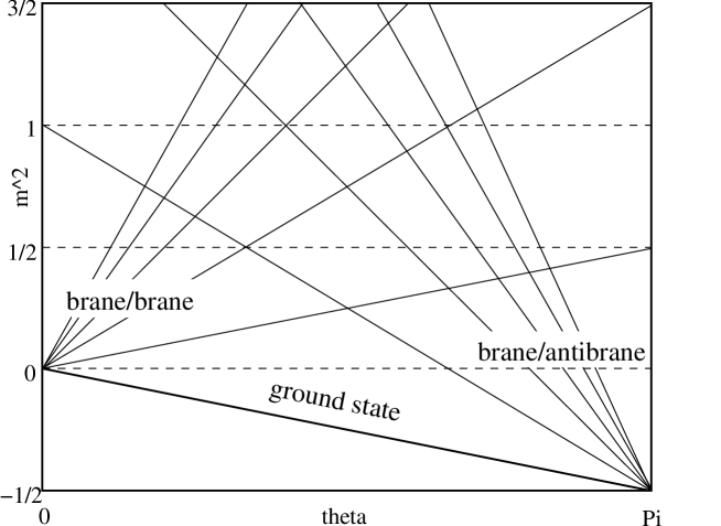
Figure 4. The ground state of the tower of lowest mass states at brane-brane configurations flows to the ground state of the tower of lowest mass states at brane-antibrane configurations, where the intersection angle $\theta$ flows from $0$ to $\pi$. The excited states of the individual towers do not match.

4.2. More tachyon actions

We will now shortly discuss other proposals for effective tachyon actions on the brane-antibrane system. An attractive option, which is reminiscent of the Abelian Born-Infeld action, is the following:

$$S=-\int d^{p+1}xV(\left|T\right|)\sqrt{-\det(\eta_{\mu\nu}+2\pi\alpha^{\prime}F_{\mu\nu}+D_{\{\mu}\overline{T}D_{\nu\}T})}$$ (4.12)

with unspecified tachyon potential $V$. This is actually a generalization of a non-BPS-brane action which had been proposed in [55] and was shown to reproduce (in the non-BPS-brane case) some S-matrix elements involving tachyon states. The Born-Infeld like tachyon action (4.12) and similar actions have been used as phenomenological field theory models of tachyon condensation [33, 35]. Although it is quite different from the simple action we have discussed in the previous section, its low-energy limit near the perturbative vacuum actually is the same. Expanding the determinant, using the standard formula $\frac{\partial}{\partial A_{ij}}\det A=\det AA^{-1}_{ij}$, we arrive at

$$S=-\int d^{p+1}xV(\left|T\right|)\left(1+\frac{1}{2}G^{\mu\nu}D_{\mu}\overline{T}D_{\nu}T+\mathcal{O}(\left|DT\right|^{4})\right)$$ (4.13)

where $G=(\eta+2\pi\alpha^{\prime}F)^{-1}_{\text{sym}}$ is the open string metric. Expanding the potential as $V(\left|T\right|)=V_{0}(1+a\left|T\right|^{2})+\mathcal{O}(\left|T\right|^{4})$ and discarding all quartic terms in the tachyon field and its derivatives, the action becomes

$$S=-\int d^{p+1}x\left(a\left|T\right|^{2}+\frac{1}{2}G^{\mu\nu}D_{\mu}\overline{T}D_{\nu}T\right)$$ (4.14)

up to constant terms and overall numerical factors. Setting the gauge fields to zero, the coefficient $a$ is determined by the requirement that the tachyon field should have $m_{T}^{2}=-1/2\alpha^{\prime}$. Thus, we have $a=-1/4$. In the low-energy limit, the open string metric $G^{\mu\nu}$ reduces to the standard Lorentzian metric and by T-dualizing we recover action (4.8) of the previous section. The discussion of the mass spectrum is identical. In this light, it seems that the mass spectrum matching for intersecting brane-antibrane is a universal feature of brane-antibrane actions rather than being model-dependent. It simply is a consequence of the specific gauge symmetry of the system and the input of the correct tachyonic mass at zero angle.

There are obviously many more ways of producing gauged brane-antibrane actions. Notably, Sen recently proposed a brane-antibrane action which is related to the Born-Infeld-type action (4.12) but takes a particularly intuitive form [32]:

$$S=-\int d^{p+1}xV(T,Y_{(1)}^{I}-Y_{(2)}^{I})\left(\sqrt{-\det\mathbf{A}_{(1)}}+\sqrt{-\det\mathbf{A}_{(2)}}\right)$$ (4.15)

where

$$\mathbf{A}_{(i)\mu\nu}=\eta_{\mu\nu}+2\pi\alpha^{\prime}F_{\mu\nu}^{i}+\partial_{\mu}Y^{I}_{(i)}\partial_{\nu}Y^{I}_{(i)}+D_{\{\mu}T^{*}D_{\nu\}}T$$ (4.16)

$$F_{\mu\nu}^{(i)}=\partial_{\mu}A^{(i)}_{\nu}-\partial_{\nu}A^{(i)}_{\mu},\quad D_{\mu}T=(\partial_{\mu}-i(A_{\mu}^{(1)}-A_{\mu}^{(2)}))T$$ (4.17)

and $A^{(i)}_{\mu}$ are the Abelian gauge fields on the brane ($i=1$) and the antibrane ($i=2$) respectively. Other than in previous examples, the transverse brane coordinates $Y_{(i)}^{I}$ are included from the beginning. The motivation for their inclusion in [32] was to allow for non-zero separation of a parallel brane-antibrane pair rather than to include the intersecting brane-antibrane case. In expanding the tachyon potential $V$ to quadratic order in $\left|T\right|$, the coefficients of the expansion are determined by the requirements that

• For $T=0$, the action should reduce to the sum of the actions on the two individual branes.

• The tachyon mass should conform with the value from the string worldsheet computation for a parallel brane-antibrane pair with non-zero separation

These requirements lead to

$$V(T,Y^{I}_{(1)}-Y^{I}_{(2)})=\tau_{p}\left[1+\frac{1}{2}\left\{\sum_{I}\left(\frac{Y^{I}_{(1)}-Y^{I}_{(2)}}{2\pi\alpha^{\prime}}\right)^{2}-\frac{1}{2\alpha^{\prime}}\right\}\left|T\right|^{2}+\mathcal{O}(\left|T\right|^{4})\right]$$ (4.18)

where $\tau_{p}$ is the tension of the individual Dp-branes. Thus, by expanding the square roots in (4.15) to lowest order in the tachyon fields and taking the low-energy limit, we once more recover the action (4.8) of the previous section. This is a further example for the universality of mass spectrum matching on the intersecting brane-antibrane system.

5. Conclusion and Discussion

In an attempt to establish a field theory description of the brane-antibrane pair intersecting at small angles we made the case for the following effective action:

$$S=-\int d^{p+1}\left(\frac{1}{4}F^{\mu\nu}F_{\mu\nu}+\frac{1}{2}D_{\mu}\overline{T}D^{\mu}T-\frac{1}{4\alpha^{\prime}}\left|T\right|^{2}\right)$$ (5.1)

This action is understood as a low-energy approximation of the brane dynamics near the perturbative vacuum. Its mass spectrum was shown to coincide perfectly with the string theory worldsheet analysis. Different generalizations of tachyon field theories to intersecting brane-antibranes were discussed and we indicated that due to the specific gauge symmetry of the system, their low-energy limit had to be the same in all cases. It would be interesting to undertake a perturbational BSFT computation with gauge fields included from the beginning. For attempts at this consider [56, 57]. In particular, the authors of [57] claimed to have performed computations up to order $\alpha^{\prime 2}$. It would be interesting to check their results (which effectively provide higher order terms in the intersection angles) against the worldsheet analysis of the string theory mass spectrum.

Local brane recombination via tachyon condensation has been proposed as a realization of the Higgs Effect in brane world models. Our analysis suggests that starting from a stable, tachyon-free D-brane configuration and then rotating some of the D-branes by a small angle, tachyon condensation can indeed be equivalently described by the standard Higgs effect in an effective gauge theory. However the case of rotating D-branes in an unstable brane-antibrane pair by a small angle is more problematic for phenomenological purposes, since in the brane-antibrane system all open string degrees of freedom disappear after the tachyon condensation. This includes in particular also the open string gauge field excitations, which means in field theory language that the gauge bosons become infinitely heavy at the end point of the tachyon condensation. Therefore this kind of open string gauge bosons in the brane-antibrane system cannot play the role of the weak vector bosons in the standard model. In [1], Hashimoto and Nagaoka showed how the simple tachyon action (5.1) could be used to realize local brane-antibrane annihilation through a backreaction from the tachyon field to the brane coordinates. However, in their analysis they assumed that only the ground state would condense. The role of higher level tachyonic modes in brane recombination/local brane-antibrane annihilation remains unexplored.

Finally, it might also be interesting to explore the consequence of the large number of tachyonic modes for brane and antibrane intersecting at small angles to inflation models in brane cosmology.

After finishing the paper we noticed the paper [58], where an expression for the tachyon potential for intersecting branes at arbitrary angles was derived in the context of boundary superstring field theory. We are grateful to N. Jones for drawing our attention to this work.

References

- [1] K. Hashimoto and S. Nagaoka, Recombination of Intersecting D-branes by Local Tachyon Condensation, (2003), hep-th/0303204.
- [2] R. Blumenhagen, L. Görlich, B. Körs and D. Lüst, Noncommutative compactifications of type I strings on tori with magnetic background flux, JHEP 10 (2000) 006, hep-th/0007024.
- [3] C. Angelantonj, I. Antoniadis, E. Dudas and A. Sagnotti, Type-I strings on magnetised orbifolds and brane transmutation, Phys. Lett. B489 (2000) 223, hep-th/0007090.
- [4] G. Aldazabal, S. Franco, L. E. Ibanez, R. Rabadan and A. M. Uranga, D = 4 chiral string compactifications from intersecting branes, J. Math. Phys. 42 (2001) 3103, hep-th/0011073.
- [5] G. Aldazabal, S. Franco, L. E. Ibanez, R. Rabadan and A. M. Uranga, Intersecting brane worlds, JHEP 02 (2001) 047, hep-ph/0011132.
- [6] R. Blumenhagen, B. Körs and D. Lüst, Type I strings with F- and B-flux, JHEP 02 (2001) 030, hep-th/0012156.
- [7] L.E. Ibanez, F. Marchesano and R. Rabadan, Getting just the standard model at intersecting branes, JHEP 11 (2001) 002, hep-th/0105155.
- [8] S. Förste, G. Honecker and R. Schreyer, Orientifolds with branes at angles, JHEP 06 (2001) 004, hep-th/0105208.
- [9] R. Blumenhagen, B. Körs, D. Lúst and T. Ott, The standard model from stable intersecting brane world orbifolds, Nucl. Phys. B616 (2001) 3, hep-th/0107138.
- [10] M. Cvetic, G. Shiu and A.M. Uranga, Three-family supersymmetric standard like models from intersecting brane worlds, Phys. Rev. Lett. 87 (2001) 201801, hep-th/0107143.
- [11] M. Cvetic, G. Shiu and A.M. Uranga, Chiral four-dimensional N = 1 supersymmetric type IIA orientifolds from intersecting D6-branes, Nucl. Phys. B615 (2001) 3, hep-th/0107166.
- [12] D. Bailin, G.V. Kraniotis and A. Love, Standard-like models from intersecting D4-branes, Phys. Lett. B530 (2002) 202, hep-th/0108131.
- [13] C. Kokorelis, New standard model vacua from intersecting branes, JHEP 09 (2002) 029, hep-th/0205147.
- [14] R. Blumenhagen, String unification of gauge couplings with intersecting D- branes, (2003), hep-th/0309146.
- [15] M. Cvetic, P. Langacker and G. Shiu, A three-family standard-like orientifold model: Yukawa couplings and hierarchy, Nucl. Phys. B642 (2002) 139, hep-th/0206115.
- [16] D. Cremades, L.E. Ibanez and F. Marchesano, Yukawa couplings in intersecting D-brane models, JHEP 07 (2003) 038, hep-th/0302105.
- [17] S.H.S. Alexander, Inflation from D - anti-D brane annihilation, Phys. Rev. D65 (2002) 023507, hep-th/0105032.
- [18] C. P. Burgess, M. Majumdar, D. Nolte, F. Quevedo, G. Rajesh and R. J. Zhang, The inflationary brane-antibrane universe, JHEP 07 (2001) 047, hep-th/0105204.
- [19] G.R. Dvali, Q. Shafi and S. Solganik, D-brane inflation, (2001), hep-th/0105203.
- [20] G. Shiu and S.H.H. Tye, Some aspects of brane inflation, Phys. Lett. B516 (2001) 421, hep-th/0106274.
- [21] C. Herdeiro, S. Hirano and R. Kallosh, String theory and hybrid inflation / acceleration, JHEP 12 (2001) 027, hep-th/0110271.
- [22] C. P. Burgess, P. Martineau, F. Quevedo, G. Rajesh and R. J. Zhang, Brane antibrane inflation in orbifold and orientifold models, JHEP 03 (2002) 052, hep-th/0111025.
- [23] J. Garcia-Bellido, R. Rabadan and F. Zamora, Inflationary scenarios from branes at angles, JHEP 01 (2002) 036, hep-th/0112147.
- [24] R. Blumenhagen, B. Körs, D. Lüst and T. Ott, Hybrid inflation in intersecting brane worlds, Nucl. Phys. B641 (2002) 235, hep-th/0202124.
- [25] T. Padmanabhan, Accelerated expansion of the universe driven by tachyonic matter, Phys. Rev. D 66 (2002) 021301, hep-th/0204150.
- [26] M. Gomez-Reino and I. Zavala, Recombination of intersecting D-branes and cosmological inflation, JHEP 0209 (2002) 020, hep-th/0207278.
- [27] R. Blumenhagen, V. Braun and R. Helling, Bound states of D(2p)-D0 systems and supersymmetric p-cycles, Phys. Lett. B510 (2001) 311, hep-th/0012157.
- [28] J. Erdmenger, Z. Guralnik, R. Helling and I. Kirsch, A World Volume Perspective on the Recombination of Intersectiong Branes, hep-th/0309043.
- [29] N. Ohta and P. K. Townsend, Supersymmetry of M-Branes at Angles, Phys. Lett. B418 (1998) 77 – 84, hep-th/9710129. A. Fujii, Y. Imaizumi and N. Ohta, Supersymmetry, Spectrum and Fate of D0-D Systems with -field, Nucl. Phys. B615 (2001) 61 – 81, hep-th/0105079, D. Bak and N. Ohta, Supersymmetric D2–anti-D2 String, Phys. Lett. B527 (2002) 131 – 141, hep-th/0112034,
- [30] J.A. Minahan and B. Zwiebach, Effective Tachyon Dynamics in Superstring Theory, (2000), hep-th/0009246.
- [31] K. Hashimoto and S. Nagaoka, Realization of Brane Descent Relations in Effective Theories, (2002), hep-th/0202079.
- [32] A. Sen, Dirac-Born-Infeld Action on the Tachyon Kink and Vortex, (2003), hep-th/0303057.
- [33] G. Gibbons, K. Hori and P. Yi, String Fluid from Unstable D-branes, (2000), hep-th/0009061.
- [34] A. Sen, Tachyon Matter, (2002), hep-th/0203265.
- [35] A. Sen, Field Theory of Tachyon Matter, (2002), hep-th/0204143.
- [36] A. Hashimoto and W.T. IV, Fluctuation Spectra of Tilted and Intersecting D-branes from the Born-Infeld Action, (1997), hep-th/9703217.
- [37] A.A. Tseytlin, On non-abelian generalization of Born-Infeld action in string theory, (1997), hep-th/9701125.
- [38] P. Koerber and A. Sevrin, The Non-Abelian open superstring effective action through order , (2001), hep-th/0108169.
- [39] P. Koerber and A. Sevrin, The Non-Abelian D-brane effective action through order , (2002), hep-th/0208044.
- [40] A. Sevrin and A. Wijns, Higher order terms in the non-Abelian D-brane effective action and magnetic background fields, JHEP 0308 (2003) 059, hep-th/0306260.
- [41] S. Nagaoka, Fluctuation Analysis of Non-Abelian Born-Infeld Action in the Background of Intersecting D-branes, (2003), hep-th/0307232.
- [42] S. Stieberger and T.R. Taylor, Non-Abelian Born-Infeld action and type I - heterotic duality. I: Heterotic F**6 terms at two loops, Nucl. Phys. B647 (2002) 49, hep-th/0207026.
- [43] S. Stieberger and T.R. Taylor, Non-Abelian Born-Infeld action and type I - heterotic duality. II: Nonrenormalization theorems, Nucl. Phys. B648 (2003) 3, hep-th/0209064.
- [44] M. Berkooz, M.R. Douglas and R.G. Leigh, Branes Intersecting at Angles, Nucl. Phys. B480 (1996) 265, hep-th/9606139.
- [45] H. Arfaei and M. Sheikh Jabbari, Different D-Brane Interactions, (1996), hep-th/9608167.
- [46] M. Sheikh Jabbari, Classification of Different Branes at Angles, (1997), hep-th/9710121.
- [47] R. Blumenhagen, L. Görlich, B. Körs and D. Lüst, Asymmetric orbifolds, noncommutative geometry and type I string vacua, Nucl. Phys. B582 (2000) 44, hep-th/0003024.
- [48] R. Rabadan, Branes at angles, torons, stability and supersymmetry, Nucl. Phys. B620 (2002) 152, hep-th/0107036.
- [49] A. Sen, (1998), hep-th/9805019.
- [50] A. Sen, Tachyon Condensation on the Brane Antibrane System, (1998), hep-th/9805170.
- [51] A. Sen, Descent Relations Among Bosonic D-Branes, (1999), hep-th/9902105.
- [52] A. Sen, Tachyon Condensation in String Field Theory, (1999), hep-th/9912249.
- [53] J.A. Minahan and B. Zwiebach, Field theory models for tachyon and gauge field string dynamics, (2000), hep-th/0008231.
- [54] D. Kutasov, M. Marino and G. Moore, Remarks on Tachyon Condensation in Superstring Field Theory, (2000), hep-th/0010108.
- [55] M.R. Garousi, Tachyon Couplings on non-BPS D-branes and Dirac-Born-Infeld action, (2000), hep-th/0003122.
- [56] P. Kraus and F. Larsen, Boundary String Field Theory of the System, (2000), hep-th/0012198.
- [57] T. Takayanagi, S. Terashima and T. Uesugi, Brane-Antibrane Action from Boundary String Field Theory, (2000), hep-th/0012210.
- [58] N. T. Jones and S. H. H. Tye, Spectral flow and boundary string field theory for angled D-branes, JHEP 0308 (2003) 037, hep-th/0307092.