Nonsinglet Sector of $c=1$ Matrix Model and $2D$ Black Hole

Extending our recent work (hep-th/0310106) we study the nonsinglet sector of $c=1$ matrix model by renormalization group analysis for a gauged matrix quantum mechanics on circle with an appropriate gauge breaking term to incorporate the effect of world-sheet vortices. The flow equations indicate BKT phase transition around the self-dual radius and the nontrivial fixed points of the flow exhibit black hole like phases for a range of temperatures beyond the self-dual point. One class of fixed point interpolate between $c=1$ for $R>1$ and $c=0$ as $R\to 0$ via black hole phase that emerges after the phase transition. The other two classes of nontrivial fixed points also develop black hole like behavior beyond $R=1$. From a thermodynamic study of the free energy obtained from the Callan-Symanzik equations we show that all these unstable phases do have negative specific heat. The thermodynamic quantities indicate that the system does undergo a first order phase transition near the Hagedorn temperature, around which the new phase is formed, and exhibits one loop finite energy correction to the Hagedorn density of states. The flow equations also suggest a deformation of the target space geometry through a running of the compactification radius where the scale is given by the dilaton. Remarkably there is a regime where cyclic flow is observed.

1 Introduction

The $c=1$ matrix model have been proved to be very powerful in describing the two-dimensional string theory to all genus, both in string perturbation theory and in a nonperturbative sense [1, 2, 3, 4]. The underlying rich structure of the non-relativistic quantum mechanics of free fermions (exhibited by the singlet sector) makes the theory solvable to a very high degree and virtually renders any quantity calculable to all orders in genus expansion. Recently the $c=1$ matrix model is realized as the effective dynamics of $D$-branes in $c=1$ non-critical string theory which exhibits the duality between $c=1$ matrix model and $2D$ quantum gravity coupled to $c=1$ matter as an exact open/closed string duality [5, 6, 7, 8, 9, 10, 11, 12, 13]. The quantum mechanics of $SU(N)$ invariant matrix variables in an inverted oscillator potential is visualized as the quantum mechanics of open string tachyons attached to $N$ unstable $D0$ branes that decays into (i.e. dual to) Liouville theory coupled to $c=1$ matter describing $2D$ closed string theory together with its $D0$ branes.

The random surfaces mapped by the $c=1$ matrix model can also be embedded in a circle of radius $R$ as a compactified Euclidean theory or equivalently as a Minkowski signature string theory at finite temperature, where the free fermion representation is not sufficient due to the active role of the angular degrees of freedom belonging to the nontrivial representation of $SU(N)$ [14, 15, 16]. From matrix quantum mechanics analysis the states in the nontrivial representation of $SU(N)$, the nonsinglet sector, are understood to correspond to vortices on the world-sheet with wave functions given by the Young Tableaux of $SU(N)$. The number of boxes counts the vortex charge. Restricting the theory only to the $SU(N)$ singlet sector gives rise to the continuum limit where the effect of the world-sheet vortices are absent and the sum over the random surfaces obey T-duality [14]. Keeping the vortices triggers Kosterlitz-Thouless phase transition at self-dual radius that breaks the $R\to 1/R$ duality symmetry. Thus the states in the nontrivial representation of $SU(N)$ are important in understanding the dynamics of the world-sheet vortices and are expected to give rise to interesting phenomena like formation of $2D$ black hole [17].

An interesting solution of the two-dimensional string theory, apart from the flat space background with linear dilaton, is the two-dimensional black hole [18, 19, 20]. Some of the early attempts to get matrix-model description of two-dimensional black hole are described in [21, 22, 23, 24, 25, 26, 27, 28]. It was partially believed that the nonperturbative formulation of two-dimensional string theory in terms of an integrable theory of noninteracting nonrelativistic fermion representation of the matrix quantum mechanics can deal issues like black hole evaporation and gravitational collapse. But it turns out to be remarkably difficult to find a matrix model description of the two-dimensional black hole due to lack of clear understanding of the target space physics of linear dilaton background in the $c=1$ matrix model. The wave equation should carry information about the black hole supplemented by the dilaton. In free fermion representation, the time-of-flight coordinate $\tau$, related to the matrix model coordinate $\lambda$ by $\lambda=\sqrt{2\mu\alpha^{\prime}}\cosh\tau$, cannot be identified with the Liouville coordinate $\phi$ although this identification arises naturally from the collective field theory approach [29, 30]. This is due to the fact that the eigenvalue coordinate $\lambda$ has no obvious geometrical interpretation on the discretized world-sheet. According to [31, 32], the correct identification is through the loop operator $W(l)$, which has a clear geometrical meaning on the world-sheet, by an integral transform. Also it has been pointed out in [33] that exact solvable structure, especially the $W(\infty)$ symmetry of the $c=1$ model makes black hole hard to describe.

One would hope to understand the situation better by working in a more general representation including the world-sheet vortices. However, the study of world-sheet vortices is hard due to lack of solvable structure. In the spherical approximation, they could be studied in dual matrix description considering discrete time [34, 35, 36]. In [16], using twisted boundary condition $\phi(2\pi R)=\Omega^{\dagger}\phi(0)\Omega$, the partition function was studied in a given representation for the standard matrix oscillator (with a stable quadratic potential). The partition function in the presence of the adjoint representation (a vortex-antivortex pair) in the double scaling limit was then studied by analytically continuing to the upside down oscillator . However, a direct analytical continuation is not possible as the standard oscillator has larger symmetry than the upside down one and does not have any information about the cut-off provided by the interaction terms in the matrix potential. Hence the analytical continuation had to be completed (in the spirit of [37]) by a suitable guess about the cut-off dependence and was argued to work at least for the adjoint representation.

Based on the above approach of connecting the world-sheet vortices with the nonsinglet states of the matrix quantum mechanics, an integrable system has been constructed which is an integrable Toda chain hierarchy interpolating between the usual $c=1$ string and the Sine-Liouville background [17]. Using the duality conjecture by Fateev, Zamolodchikov and Zamolodchikov (FZZ) [39], it was proposed to be a matrix model (the KKK model) for two-dimensional black hole at $R=3/2$ that relates the two-dimensional black hole background ($SL(2,R)/U(1)$ coset CFT) to the condensation of vortices (interpreted as the winding modes around the Euclidean time). The effect of the winding modes on the world-sheet were incorporated in the matrix quantum mechanics path integral by integrating over the twist variables (the matrix holonomy factor around the compactification circle) along with an appropriate measure and the twisted partition function. The FZZ correspondence allows one to consider the winding mode condensation from the Sine-Liouville side to construct the appropriate matrix model for the black hole background, avoiding dealing directly more complicated black hole geometry. However, not considering the black hole background directly has some disadvantages for the following reason. Although FZZ conjecture has been tested by calculating various correlators, it is not clear how to get information about the black hole metric from the Sine-Liouville side. On the other hand, considering the thermodynamics of two-dimensional string theory above the temperature corresponding to the Berezinski-Kosterlitz-Thouless (BKT) phase transition [40, 41, 42], it has been proposed [17] that the nonsinglet states (or the vortices on the world-sheet) fills the Hagedorn density of black holes $\rho(E)\sim E^{-s_{1}}e^{\beta_{H}E}$, since the perturbative spectrum of two-dimensional string theory has very few states, namely the massless tachyon. The Hagedorn spectrum of states should then be obtained by a direct counting of the nonsinglet states in the $c=1$ matrix model. From a Hamiltonian point of view, to count the states in a given energy interval one needs to diagonalize the Hamiltonians for representations corresponding to the large Young tableaux. This is difficult due to Calogero type of interaction of the eigenvalues with the $SU(N)$ spin structure. Also, there are other important questions like understanding black hole phases at any radius other than the fixed radius $R=3/2$ (to which the unstable black hole can decay to), the possibility of observing Hawking radiation and the like.

The main motivation of the present paper is to address above questions from an explicit study of the nonsinglet sector and the BKT phase transition directly from the matrix quantum mechanics path integral with periodic boundary condition. Instead of working in any particular representation let us have recourse to the renormalization group approach that we developed in a recent paper [13] for the $c=1$ matrix model on a circle of radius $R$. There we described a detail analysis of how the two coupling constants in the double scaling limit with critical exponent flow with the change in length scale. The motivation came from an earlier work of Brézin and Zinn-Justin [43] on large $N$ RG analysis of $c=0$ matrix model. The scheme reproduces the known results of the solvable sub-sector of the matrix quantum mechanics, namely a non-trivial fixed point with the correct string susceptibility exponent of the $c=1$ model, T-dulaity and the expected logarithmic scaling violation of the free energy. Also it exhibits, qualitatively, the physically interesting situations due to the effects of nonsinglet sector, which can not be simplified because of the lack of the solvable structure. For example, from the running of the prefactor of the partition function, written in the renormalized couplings, analogous to the running due to the wave function renormalization, the free energy is observed to change sign near $R=1$ for small value of the critical coupling. This is reminiscent of the BKT transition at self-dual radius triggered by the liberation of the world-sheet vortices. We would like to understand the detail nature of the nontrivial fixed points of the flow that describes the physics beyond this transition.

To capture the effect of vortices on the flows and the fixed points more clearly and to introduce a new coupling that would act like vortex fugacity, in this paper we analyze the behavior of the following gauged matrix model with simple periodic boundary condition and with an appropriate gauge breaking term

$$\mathcal{Z}_{N}[g,\alpha,R]=\int_{\phi_{N}(2\pi R)=\phi_{N}(0)}\mathcal{D}^{(N)^{2}}A_{N}(t)~{}\mathcal{D}^{(N)^{2}}\phi_{N}(t)$$

$$\exp\Big{[}-(N)~{}\mbox{Tr}\int_{0}^{2\pi R}dt~{}\Big{\{}\frac{1}{2}(D\phi_{N}(t))^{2}+\frac{1}{2}\phi_{N}^{2}(t)-\frac{g}{3}\phi_{N}^{3}(t)+\frac{A_{N}^{2}}{\alpha}\Big{\}}\Big{]}\,,$$

(1.1)

where the covariant derivative $D$ is defined with respect to the pure gauge $A(t)=\Omega(t)^{\dagger}\dot{\Omega}(t)$ by $D\phi=\partial_{t}\phi+[A,\phi]$. Unlike taking the course of integration over the twist fields with a proper measure incorporating winding modes around the Euclidean time in the path integral (as considered in [17]), here the integration over the gauge field $A(t)=\Omega^{\dagger}\dot{\Omega}(t)$ with an appropriate measure provided by the gauge breaking term inserts world-sheet vortices in the partition function where $\alpha$ acts as the vortex fugacity. This can happen through the insertion of operator of the form $\exp(-\alpha J^{2})$ that counts vortex number, where $J^{2}\sim nN$. Without the gauge breaking term the system is projected to the singlet sector. We observe that one class of nontrivial fixed points of the flow give rise to a pair of $c=1$ fixed points at large $R$ with one unstable direction. As $R$ is decreased the flow passes through Kosterlitz-Thouless phase transition at $R=1.03$, where the operators coupled to the vortex fugacity become relevant indicating the liberation of the world-sheet vortices as expected at the self dual radius $R=1$ [15]. Between $0.67\leq R\leq 0.7$ the pair of fixed points become purely repulsive fixed points of large coupling and exhibit negative specific heat and one loop correction to the Hagedorn density of states very similar to those exhibited by an unstable Euclidean black hole in flat space time. The change of entropy exhibits a discontinuity at $R=0.73$, little above the BKT temperature, indicating the Hagedorn transition to be first order. As $R$ is further decreased the flow ends up into a pair of $c=0$ fixed points. The other two classes of fixed points also show black hole like behavior beyond the BKT phase transition. This indicates he existence of other black hole phases at other radii of compactification. Also a running of the compactification radius with the scale, thought as dilaton, suggests a deformation of the target space geometry that might be crucial to visualize those black holes. We observe cyclic flow below the BKT temperature presumably due to resonance of high spin states indicating stringy behavior [44]. In fact, beyond the phase transition, where different nontrivial fixed points exhibit black hole like behavior, the cycles become very complicated. The phase structure probed by the RG analysis thus remarkably captures the expected properties and looks promising in understanding the much unexplored physics of the nonsinglet sector. The dynamics in the neighborhood of the black hole like fixed point needs to be studied in detail to understand its explicit nature. In this paper we will motivate such studies regarding the role of the nonsinglet sector from the observations from our Renormalization group analysis.

The plan of the paper is as follows. In section 2 we describe the RG calculation for our model (1.1). In section 3 we analyze the flow and discuss the phase structure. We observe the BKT phase transition near the self dual radius (or a Hagedorn transition little below the BKT radius) and existence of a black hole like fixed point past the transition. In section 4 we analyze the thermodynamics of the black hole like fixed point and comment on the sense in which it resembles the thermodynamics of an unstable (thermal) Euclidean black hole. In section 5 we conclude with discussion and open questions.

2 The Large $N$ RG Calculation

In this section we will summarize the renormalization group calculation for the $c=1$ gauged matrix model on a circle, with a gauge breaking term appropriate for capturing the nonsinglet physics. The details of the method for the ungauged model with periodic boundary condition is studied in [13].

Let us consider the partition function for the $N+1$ dimensional matrix variables

$$\mathcal{Z}_{N+1}[g,\alpha,R]=\int_{\phi_{N+1}(2\pi R)=\phi_{N+1}(0)}\mathcal{D}^{(N+1)^{2}}A_{N+1}(t)~{}\mathcal{D}^{(N+1)^{2}}\phi_{N+1}(t)$$

$$\exp\Big{[}-(N+1)~{}\mbox{Tr}\int_{0}^{2\pi R}dt~{}\Big{\{}\frac{1}{2}(D\phi_{N+1}(t))^{2}+\frac{1}{2}\phi_{N+1}^{2}(t)-\frac{g}{3}\phi_{N+1}^{3}(t)+\frac{A_{N+1}^{2}}{\alpha}\Big{\}}\Big{]}\,.$$

(2.1)

The covariant derivative $D$ and the gauge field $A(t)$ are defined respectively as

$$D\phi=\partial_{t}\phi+[A,\phi]\,,~{}~{}~{}~{}A(t)=\Omega(t)^{\dagger}\dot{\Omega}(t)\,,~{}~{}~{}~{}\Omega\in U(N)\,.$$ (2.2)

Expanding the covariant derivative, the partition function is rewritten as

$$\mathcal{Z}_{N+1}[g,\alpha,R] = \int_{\phi_{N+1}(2\pi R)=\phi_{N+1}(0)}\mathcal{D}^{(N+1)^{2}}A_{N+1}(t)~{}\mathcal{D}^{(N+1)^{2}}\phi_{N+1}(t)$$

$$\exp\Big{[}-(N+1)\mbox{Tr}\int_{0}^{2\pi R}dt~{}\Big{\{}\frac{1}{2}\dot{\phi}_{N+1}(t)^{2}+\frac{1}{2}\phi_{N+1}^{2}(t)-\frac{g}{3}\phi_{N+1}^{3}(t)$$

$$+A_{N+1}(t)~{}[\phi_{N+1}(t),\dot{\phi}_{N+1}(t)]+\frac{1}{2}~{}[A_{N+1}(t),\phi_{N+1}(t)]^{2}+\frac{A_{N+1}^{2}}{\alpha}\Big{\}}\Big{]}\,.$$

The $A_{N+1}(t)[\phi_{N+1}(t),\dot{\phi}_{N+1}(t)]$ term above is crucial to study the nonsinglets. Even though they are present, the gauge invariance tries to project the system to the singlet sector while the gauge breaking term prevents to do so. In [14], a finitely large radius representation of singlet sector was obtained by throwing this particular term by hand as the nonsinglets are confined at small temperature. In [16], the partition function for one vortex/anti-vortex pair, i.e. in the adjoint representation was calculated by analytical continuation from the twisted partition function of the standard harmonic oscillator to that of the upside down oscillator. For $\alpha=0$, the gauge fields are forced to vanish and the partition function reduces to that of ungauged matrix quantum mechanics on circle.

Because of the gauge breaking term, the integration over all possible configurations of $A(t)$ formally inserts (the gauge invariant) operator $\exp\mbox{Tr}(-\alpha J^{2})$ in the partition function,

$$\int dA~{}\exp\mbox{Tr}\Big{(}-\frac{A^{2}}{\alpha}+2iAJ\Big{)}~{}\sim~{}\exp(-\alpha J^{2})~{}\sim~{}\exp(-N\alpha n)\,.$$ (2.4)

Here $J^{2}$ is proportional to the quadratic Casimir invariant $C(n)\approx Nn$. Characterizing the irreducible representations in terms of the number of the white boxes $n$ in the Young tableaux, the quadratic Casimir only depends on $n$ to the leading order in $N$. The reason for this behavior is that, $\exp\mbox{Tr}(-\alpha J^{2})$ acts on the states $|\mbox{Adj}\rangle$ in the adjoint representation (belonging to the nonsinglet sector) of the MQM in the gauge invariant way,

$$A\cdot J|\mbox{Adj}\rangle^{n}=\alpha~{}n|\mbox{Adj}\rangle^{n}\,.$$ (2.5)

The parameter $\alpha$ behaves like the fugacity of vortices. The operator $\exp\mbox{Tr}(-\alpha J^{2})$ therefore counts the vortex number.

2.1 Integrating out a column and a row of the matrices:

Now we decompose the $(N+1)\times(N+1)$ matrices into $N\times N$ blocks and $N$-vectors and scalars as follows

$$\phi_{N+1}(t)=\begin{pmatrix}\phi_{N}(t)&v_{N}(t)\cr v^{*}_{N}(t)&\epsilon\cr\end{pmatrix}\,,$$ (2.6)

and

$$A_{N+1}(t)=\begin{pmatrix}A_{N}(t)&a_{N}(t)\cr a^{*}_{N}(t)&\eta\cr\end{pmatrix}\,.$$ (2.7)

The scalars $\epsilon$ and $\eta$ are of relative order $1/N$ and can be ignored in the double scaling limit. Even though the matrix elements are not independent ($\phi$ being hermitian and $A$ being antihermitian) one can always choose such decomposition for each value of $N$ which does not prevent the action to be written in the same form in terms of the covariant derivatives. The resulting partition function can be written as

$$\mathcal{Z}_{N}[g,\alpha,R] = \int_{\phi_{N}(2\pi R)=\phi_{N}(0)}\mathcal{D}^{N^{2}}A_{N}(t)~{}\mathcal{D}^{N^{2}}\phi_{N}(t)$$ (2.8)

$$\exp\Big{[}-(N+1)~{}\mbox{Tr}\int_{0}^{2\pi R}dt~{}\Big{\{}\frac{1}{2}\dot{\phi}_{N}(t)^{2}+\frac{1}{2}\phi_{N}^{2}(t)-\frac{g}{3}\phi_{N}^{3}(t)$$

$$+A_{N}(t)~{}[\phi_{N}(t),\dot{\phi}_{N}(t)]+\frac{1}{2}~{}[A_{N}(t),\phi_{N}(t)]^{2}+\frac{A_{N}^{2}}{\alpha}\Big{\}}\Big{]}\,.$$

$$\times\int_{v,v^{*}(2\pi R)=v,v^{*}(0)}\mathcal{D}^{N}a(t)\mathcal{D}^{N}a^{*}(t)\mathcal{D}^{N}v(t)\mathcal{D}^{N}v^{*}(t)$$

$$\exp\Big{[}-(N+1)\int_{0}^{2\pi R}dt~{}\Big{\{}\dot{v}^{*}\dot{v}+\dot{v}^{*}A_{N}v-v^{*}A_{N}\dot{v}+v^{*}(A_{N}^{2}+1-g\phi_{N})v$$

$$+a^{*}\Big{(}\phi_{N}^{2}+\frac{1}{\alpha}\Big{)}a+v^{*}(\dot{\phi}_{N}+2A_{N}\phi_{N}-\phi_{N}A_{N})a-\dot{v}^{*}\phi_{N}a$$

$$+a^{*}(-\dot{\phi}_{N}+2\phi_{N}A_{N}-A_{N}\phi_{N})v+a^{*}\phi_{N}\dot{v}$$

$$+a^{*}va^{*}v+v^{*}av^{*}a-v^{*}va^{*}a-a^{*}vv^{*}a\Big{\}}\Big{]}\,.$$

Rescaling the vectors $v(t)\rightarrow\frac{v(t)}{\sqrt{2\pi R(N+1)}}$ and $a(t)\rightarrow\frac{a(t)}{\sqrt{2\pi R(N+1)}}$, the $v$ and $a$ dependent part of the partition function turns out to be

$$I[g,\alpha,\phi_{N},A_{N},R] = \frac{1}{(\sqrt{2\pi R(N+1)})^{4N}}\int_{v,v^{*}(2\pi R)=v,v^{*}(0)}\mathcal{D}^{N}a(t)\mathcal{D}^{N}a^{*}(t)\mathcal{D}^{N}v(t)\mathcal{D}^{N}v^{*}(t)$$ (2.9)

$$\exp\Big{[}-\int_{0}^{2\pi R}\frac{dt}{2\pi R}~{}\Big{\{}\dot{v}^{*}\dot{v}+\dot{v}^{*}A_{N}v-v^{*}A_{N}\dot{v}+v^{*}(A_{N}^{2}+1-g\phi_{N})v$$

$$+a^{*}\Big{(}\phi_{N}^{2}+\frac{1}{\alpha}\Big{)}a+v^{*}(\dot{\phi}_{N}+2A_{N}\phi_{N}-\phi_{N}A_{N})a-\dot{v}^{*}\phi_{N}a$$

$$+a^{*}(-\dot{\phi}_{N}+2\phi_{N}A_{N}-A_{N}\phi_{N})v+a^{*}\phi_{N}\dot{v}$$

$$+\frac{1}{2\pi R(N+1)}(a^{*}va^{*}v+v^{*}av^{*}a-v^{*}va^{*}a-a^{*}vv^{*}a)\Big{\}}\Big{]}\,.$$

Using the following Fourier transformation

$$\mathcal{O}(t)=\sum_{m=-\infty}^{\infty}\mathcal{O}_{m}~{}e^{i\frac{m}{R}t}\,,~{}~{}~{}\mathcal{O}_{m}=\int_{0}^{2\pi R}\frac{dt}{2\pi R}~{}e^{-i\frac{m}{R}t}\mathcal{O}(t)\,,$$ (2.10)

with

$$\delta_{mn}=\int_{0}^{2\pi R}\frac{dt}{2\pi R}~{}e^{i\frac{(n-m)}{R}t}\,,~{}~{}~{}\delta(t-t^{\prime})=\frac{1}{2\pi R}\sum_{m=-\infty}^{\infty}e^{i\frac{m}{R}(t-t^{\prime})}\,,$$

the $(v,a)$-integration can be expressed as

$$I[g,\alpha,\phi_{N},A_{N},R]=\frac{1}{(\sqrt{2\pi R(N+1)})^{4N}}\int\Big{(}\prod_{m}da_{m}^{*}da_{m}^{*}\Big{)}\Big{(}\prod_{m}dv_{n}^{*}dv_{n}^{*}\Big{)}$$

$$\exp\Big{\{}-\sum_{m}\Big{(}v_{m}^{*}\Big{(}\frac{m^{2}}{R^{2}}+1\Big{)}v_{m}+\frac{a_{m}^{*}a_{m}}{\alpha}\Big{)}\Big{\}}$$

$$\exp\Big{\{}-\sum_{m,l}v_{m}^{*}\Big{(}-i\frac{m}{R}A_{m-l}-i\frac{l}{R}A_{m-l}+\sum_{k}A_{m-l-k}A_{k}-g\phi_{m-l}\Big{)}v_{l}\Big{\}}$$

$$\exp\Big{\{}-\sum_{m,l}a_{m}^{*}(\sum_{k}\phi_{m-l-k}\phi_{k})a_{l}\Big{\}}$$

$$\exp\Big{\{}-\sum_{m,l}v_{m}^{*}\Big{(}i\frac{(m-l)}{R}\phi_{m-l}+i\frac{m}{R}\phi_{m-l}+2\sum_{k}A_{m-l-k}\phi_{k}-\sum_{k}\phi_{m-l-k}A_{k}\Big{)}a_{l}\Big{\}}$$

$$\exp\Big{\{}-\sum_{m,l}a_{m}^{*}\Big{(}i\frac{(m-l)}{R}\phi_{m-l}+i\frac{m}{R}\phi_{m-l}+2\sum_{k}\phi_{m-l-k}A_{k}-\sum_{k}A_{m-l-k}\phi_{k}\Big{)}v_{l}\Big{\}}\,,$$

where we have neglected the $O(1/N)$ terms. The above integration, as an extra piece to the matrix integral, contains the vectors $v(t)$ (or quarks) generating boundaries on the Feynman diagrams. In fact in vanishing $\alpha$ limit, this is essentially equivalent to the model considered in [45, 46, 13]. For generic value of $\alpha$, the above integral should insert nonsinglet boundaries on the world-sheet that arise after the BKT phase transition.

2.2 One loop Feynman diagrams

In order to carry out the $v$ and $a$ integration diagrammatically, let us now define the following operators

$$\mathcal{O}_{mn}^{v^{*}v} = \Big{(}\frac{mn}{R^{2}}+1\Big{)}\delta_{mn}\,,~{}~{}~{}\mathcal{O}_{mn}^{a^{*}a}(\alpha)=\frac{\delta_{mn}}{\alpha}\,,$$

$$\mathcal{O}_{m-l}^{v^{*}v}(g,\phi,A) = \Big{(}-i\frac{(m+l)}{R}A_{m-l}+\sum_{k}A_{m-l-k}A_{k}-g\phi_{m-l}\Big{)}\,,$$

$$\mathcal{O}_{m-l}^{a^{*}a}(\phi) = \Big{(}\sum_{k}\phi_{m-l-k}\phi_{k}\Big{)}\,,$$

$$\mathcal{O}_{m-l}^{v^{*}a}(\phi,A) = \Big{(}i\frac{(2m-l)}{R}\phi_{m-l}+2\sum_{k}A_{m-l-k}\phi_{k}-\sum_{k}\phi_{k}A_{m-l-k}\Big{)}\,,$$

$$\mathcal{O}_{m-l}^{a^{*}v}(\phi,A) = \Big{(}i\frac{(2l-m)}{R}\phi_{m-l}+2\sum_{k}\phi_{k}A_{m-l-k}-\sum_{k}A_{m-l-k}\phi_{k}\Big{)}\,.$$ (2.12)

The inverse of these operators define various propagators and vertices according to figure 1.

Figure 1: The propagators and vertices.

Hence the integral becomes

$$I[g,\alpha,\phi_{N},A_{N},R,N] = \frac{1}{(2\pi R(N+1))^{2N}}~{}\exp\Big{[}-\{\sum_{m_{1},l_{1}}(\mathcal{O}_{m_{1}-l_{1}}^{v^{*}v}(g,\phi,A))^{-1}$$ (2.13)

$$+\sum_{m_{2},l_{2}}(\mathcal{O}_{m_{2}-l_{2}}^{a^{*}a}(\phi))^{-1}+\sum_{m_{3},l_{3}}(\mathcal{O}_{m_{3}-l_{3}}^{a^{*}v}(\phi,A))^{-1}$$

$$+\sum_{m_{4},l_{4}}(\mathcal{O}_{m_{4}-l_{4}}^{v^{*}a}(\phi,A))^{-1}\}\Big{]}~{}I_{0}(\alpha,R,N)\,,$$

where the gaussian part is as follows

$$I_{0}[\alpha,R,N]=\int\Big{(}\prod_{i}da_{i}^{*}da_{i}\Big{)}\Big{(}\prod_{j}dv_{j}^{*}dv_{j}\Big{)}~{}\exp\big{[}-\sum_{m}(v_{m}^{*}\mathcal{O}_{mm}^{v^{*}v}v_{m}+a_{m}^{*}\mathcal{O}_{mm}^{a^{*}a}a_{m})\big{]}\,.$$ (2.14)

Performing the gaussian integration, we get

$$I_{0}[\alpha,R,N]=(2\pi R)^{2N}\pi^{2N}\exp\Big{[}-\mbox{Tr}\Big{\{}\sum_{m}\ln\Big{(}\frac{m^{2}}{R^{2}}+1\Big{)}{\bf 1}\Big{\}}\Big{]}\exp\Big{[}-\mbox{Tr}\Big{\{}\ln\Big{(}\frac{1}{\alpha}\Big{)}{\bf 1}\Big{\}}\Big{]}\,.$$ (2.15)

Inserting this into (2.13), the $(v,a)$-integration becomes

$$I[g,\alpha,\phi_{N},A_{N},R,N]=\mathcal{C}(\alpha,R,N)~{}\Sigma[g,\alpha,\phi_{N},A_{N},R,N]\,,$$ (2.16)

where

$$\mathcal{C}(\alpha,R,N)=\bigg{[}\frac{\pi^{3}R\alpha}{(N+1)^{2}\sinh\pi R}\bigg{]}^{N}~{}\frac{1}{\prod_{m}(m/R)^{2N}}\,.$$ (2.17)

In (2.16), $\Sigma[g,\alpha,\phi_{N},A_{N},R,N]$ represents sum of one loop Feynman diagrams as shown in figure 2.

Figure 2: The one loop diagrams contributing to $\Sigma$.

2.3 Evaluation of the diagrams

We evaluate the diagrams to express $\Sigma[g,\alpha,\phi_{N},A_{N},R,N]$ as a series expansion in the couplings, $g$, $\alpha$, and the Fourier modes of the fields $\phi_{m}$, $A_{m}$. The full series expansion is given in the Appendix A. We will now discuss how to express this series into an expansion in $g$, $\alpha$, $\Phi(t)$ and $A(t)$ by suitable inverse Fourier transform.

In order to evaluate the one loop correction to the effective action, we inverse transform the Fourier modes according to the rule (2.10) and sum-up the set of infinite series using the formulae discussed below.

$$\sum_{m=-\infty}^{\infty}\frac{\exp[i(m/R)t]}{\frac{m^{2}}{R^{2}}+a^{2}} = \frac{\pi R}{a}\frac{\cosh(\pi aR-at)}{\sinh\pi aR}\,,~{}~{}~{}0\leq t\leq 2\pi R\,,$$

$$\sum_{m=-\infty}^{\infty}\frac{m/R~{}\exp[i(m/R)t]}{\frac{m^{2}}{R^{2}}+a^{2}} = \frac{i\pi R~{}\sinh(\pi aR-at)}{\sinh\pi aR}\,,~{}~{}~{}0<t<2\pi R\,,$$ (2.18)

$$i\pi R\,,~{}~{}~{}~{}~{}~{}~{}~{}~{}~{}~{}~{}~{}~{}~{}~{}~{}~{}~{}~{}~{}~{}~{}~{}~{}~{}t\to 0\,,$$

$$-i\pi R\,,~{}~{}~{}~{}~{}~{}~{}~{}~{}~{}~{}~{}~{}~{}~{}~{}~{}~{}~{}~{}~{}~{}~{}t\to 2\pi R\,,$$

$$0\,,~{}~{}~{}~{}~{}~{}~{}~{}~{}~{}~{}~{}~{}~{}~{}~{}~{}~{}~{}~{}~{}~{}~{}~{}~{}~{}t=0=2\pi R\,.$$

Because of the discontinuity in the last series shown above, all other series, which look like higher derivatives of the above functions, has delta function or derivative of delta function like behavior. This behavior actually dominate over the regular part of those functions and hence dominate the contribution when the functions are integrated over :

$$\sum_{m=-\infty}^{\infty}\frac{m^{2}/R^{2}~{}\exp[i(m/R)t]}{\frac{m^{2}}{R^{2}}+a^{2}} \sim 2\pi R\delta(t)\,,~{}~{}~{}0\leq t\leq 2\pi R\,,$$

$$\sum_{m=-\infty}^{\infty}\frac{m^{3}/R^{3}~{}\exp[i(m/R)t]}{\frac{m^{2}}{R^{2}}+a^{2}} \sim -2\pi iR\delta^{\prime}(t)\,,~{}~{}~{}0<t<2\pi R\,,$$

$$\sum_{m=-\infty}^{\infty}\frac{m^{4}/R^{4}~{}\exp[i(m/R)t]}{\frac{m^{2}}{R^{2}}+a^{2}} \sim -2\pi R\delta^{\prime\prime}(t)\,,~{}~{}~{}0\leq t\leq 2\pi R\,.$$ (2.19)

One way to see the above behavior is as follows:

$$\sum_{m=-\infty}^{\infty}\frac{m^{2}/R^{2}~{}\exp[i(m/R)t]}{\frac{m^{2}}{R^{2}}+a^{2}} \sim \sum_{m=-\infty}^{\infty}\exp[i(m/R)t]=2\pi R\delta(t)\,,~{}~{}~{}0\leq t\leq 2\pi R\,,$$

$$\sum_{m=-\infty}^{\infty}\frac{m^{2}/R^{2}}{\frac{m^{2}}{R^{2}}+a^{2}} \sim \sum_{m=-\infty}^{\infty}1=2\pi R\delta(0)\,.$$ (2.20)

Also

$$\sum_{m=-\infty}^{\infty}\frac{m^{3}/R^{3}~{}\exp[i(m/R)t]}{\frac{m^{2}}{R^{2}}+a^{2}} \sim \sum_{m=-\infty}^{\infty}\frac{m}{R}~{}\exp[i(m/R)t]=-2\pi iR\delta^{\prime}(t)\,,~{}~{}~{}0<t<2\pi R\,,$$

$$\sum_{m=-\infty}^{\infty}\frac{m^{3}/R^{3}}{\frac{m^{2}}{R^{2}}+a^{2}} \sim \sum_{m=-\infty}^{\infty}\frac{m}{R}=0\,,$$

$$\sum_{m=-\infty}^{\infty}\frac{m^{4}/R^{4}~{}\exp[i(m/R)t]}{\frac{m^{2}}{R^{2}}+a^{2}} \sim \sum_{m=-\infty}^{\infty}\frac{m^{2}}{R^{2}}~{}\exp[i(m/R)t]=-2\pi R\delta^{\prime\prime}(t)\,,~{}~{}~{}0\leq t\leq 2\pi R\,.$$

$$\sum_{m=-\infty}^{\infty}\frac{m^{4}/R^{4}}{\frac{m^{2}}{R^{2}}+a^{2}} \sim \sum_{m=-\infty}^{\infty}\frac{m^{2}}{R^{2}}=-2\pi R\delta^{\prime\prime}(0)\,.$$ (2.21)

Note that while integrating over these functions, we have to take into account their periodic nature and the intervals over which they are defined. We also have to deal with subtleties when these intervals are strictly inequalities.

These sums give the corrections to the coefficients of the various terms in the action, after $\Sigma[g,\alpha,\phi_{N},A_{N},R,N]$ is exponentiated and log-expanded around $\phi=0$ (small field approximation). Since after doing the inverse Fourier transform, the various terms containing $\phi(t)$ and $A(t)$ has nonlocal integrals over several one dimensional dummy time variables, we breakup the variables into center of mass and relative coordinates. Then we expand the functions about the center of mass coordinates, assuming the relative coordinates to be small enough, and consider integration over the relative coordinates.

Now taking into account all these considerations, after evaluating the integrations over relative time variables (see Appendix B), the expression for $\Sigma[g,\alpha,\phi_{N},A_{N},R,N]$ becomes

$$\Sigma[g,\alpha,\phi_{N},A_{N},R,N]=1+F_{g1}(R)~{}g\int_{0}^{2\pi R}dt~{}\mbox{Tr}\phi(t)$$

$$+\{F_{g2}(R)~{}g^{2}+F_{\alpha 2}(R)~{}\alpha\}\int_{0}^{2\pi R}dt~{}\mbox{Tr}\frac{1}{2}\phi^{2}(t)+\{\hat{F}_{g2}(R)~{}g^{2}+\hat{F}_{\alpha 2}(R)~{}\alpha\}\int_{0}^{2\pi R}dt~{}\mbox{Tr}\frac{1}{2}\dot{\phi}^{2}(t)$$

$$+G_{2}(R)\int_{0}^{2\pi R}dt~{}\mbox{Tr}A^{2}(t)+\{G_{g3}(R)~{}g^{2}+G_{\alpha 3}(R)\alpha\}\int_{0}^{2\pi R}dt~{}\mbox{Tr}A(t)\phi(t)\dot{\phi}(t)$$

$$+\{G^{\prime}_{g3}(R)~{}g^{2}+G^{\prime}_{\alpha 3}(R)\alpha\}\int_{0}^{2\pi R}dt~{}\mbox{Tr}A(t)\dot{\phi}(t)\phi(t)+\{F_{g3}(R)~{}g^{3}$$

$$+F_{\alpha g3}(R)~{}\alpha g\}\int_{0}^{2\pi R}dt~{}\mbox{Tr}\frac{1}{3}\phi^{3}(t)+\{G_{\alpha 4}(R)~{}\alpha+G_{g4}(R)~{}g^{2}\}\int_{0}^{2\pi R}dt~{}\mbox{Tr}A(t)\phi(t)A(t)\phi(t)$$

$$+\{G^{\prime}_{\alpha 4}(R)~{}\alpha+G^{\prime}_{g4}(R)~{}g^{2}\}\int_{0}^{2\pi R}dt~{}\mbox{Tr}A^{2}(t)\phi^{2}(t)\,.$$

The functions $F(R)$s and $G(R)$s are defined as follows

$$F_{g1}(R) = \coth\pi R\,,~{}~{}~{}~{}F_{g2}(R)=\frac{\pi R}{2}(1+\coth^{2}\pi R)+\frac{1}{2}\coth\pi R\cosh 2\pi R$$

$$F_{\alpha 2}(R) = -1/(\pi R)+8-4\coth\pi R\,,~{}~{}~{}~{}\hat{F}_{\alpha 2}(R)=-4\coth\pi R\,,$$

$$\hat{F}_{g2}(R) = \frac{1}{\sinh^{2}\pi R}\big{(}\frac{1}{64}(1+8\pi^{2}R^{2})\sinh 4\pi R-\frac{\pi^{3}R^{3}}{6}\cosh 2\pi R-\frac{\pi R}{16}\cosh 4\pi R\big{)}\,,$$

$$G_{2}(R) = -3\coth\pi R+\frac{\pi R}{2\sinh^{2}\pi R}-\frac{\pi R}{2}(1+\coth^{2}\pi R)\,,$$

$$F_{g3}(R) = \frac{\pi R}{64\sinh^{3}\pi R(\cosh 2\pi R+\cosh 4\pi R)}[4\pi R(3\cosh\pi R+2\cosh 3\pi R+2\cosh 5\pi R$$

$$+\cosh 7\pi R)+\sinh\pi R+\sinh 5\pi R+2\sinh 7\pi R+\sinh 9\pi R]\,,$$

$$F_{\alpha g3}(R) = \frac{39\pi R}{4}(1+\coth^{2}\pi R)-\frac{33}{4}\coth\pi R\,,$$

$$G_{g3}(R) = G_{g3}^{\prime}(R)=\frac{1}{12}(\pi R\cosh 2\pi R-\frac{1}{2}\sinh 2\pi R)\,,$$

$$G_{g4}(R) = -\frac{1}{8\sinh^{2}\pi R}\big{(}\pi^{2}R^{2}\cosh 3\pi R+\frac{\pi R}{8}\sinh 5\pi R+\frac{\pi R}{4}\sinh 3\pi R-\frac{3}{8}\sinh\pi R\big{)}\,,$$

$$G_{\alpha 3}(R) = G_{\alpha 3}^{\prime}(R)=-\frac{2}{3}\coth\pi R+\frac{1}{\sinh^{2}\pi R}(\frac{\pi R}{6}\cosh\pi R+\frac{1}{12}\sinh\pi R)\,,$$

$$G_{\alpha 4}(R) = -2\coth\pi R\,,~{}~{}~{}~{}G_{\alpha 4}^{\prime}(R)=\frac{5}{2}\coth\pi R\,,~{}~{}~{}~{}G_{g4}^{\prime}(R)=0\,.$$ (2.23)

2.4 Elimination of the tadpole term

The term proportional to $\int_{0}^{2\pi R}dt~{}\phi(t)$ is unwanted. To remove this term, we change the background by $\phi(t)\to\phi(t)+f$, and set the net coefficient of the linear term to zero. This fixes the value of $f$ to be

$$f_{\pm} = \frac{1}{2}\Big{(}g+\frac{g}{N}+\frac{\alpha gF_{\alpha g3}+g^{3}F_{g3}}{N}\Big{)}^{-1}\Big{[}\Big{(}1+\frac{1}{N}-\frac{\alpha F_{\alpha 2}+g^{2}F_{g2}}{N}\Big{)}$$ (2.24)

$$\pm\Big{\{}\Big{(}1+\frac{1}{N}-\frac{\alpha F_{\alpha 2}+g^{2}F_{g2}}{N}\Big{)}^{2}-\frac{4gF_{g1}}{N}\Big{(}g+\frac{g}{N}+\frac{\alpha gF_{\alpha g3}+g^{3}F_{g3}}{N}\Big{)}\Big{\}}^{\frac{1}{2}}\Big{]}$$

As $f_{+}\sim O(1)$ and $f_{-}\sim O(1/N)$, we choose the smaller shift

$$f_{-}\sim gF_{g1}/N$$ (2.25)

to suppress the contribution from the higher order terms. Note that the coefficient of $\phi^{n}(t)$ term would contribute a term proportional to $f$ in the coefficient of $\phi^{n-1}(t)$ term. Thus the coefficient of $\phi^{3}(t)$ in the coupling $g_{3}$ would have an $O(1/N)$ contribution in the coupling $g_{4}$ from the $\phi^{4}(t)$ term, if we had turned it on. Also the contribution from the $[A(t),\phi(t)]^{2}$ term in the coefficient of the $A^{2}(t)$ term can be ignored as it is of $O(1/N^{2})$. After accommodating all such changes, the expression for $Z_{N+1}$ becomes

$$Z_{N+1}=\mathcal{C}(\alpha,R,N)~{}\exp[2\pi RN^{2}\mathscr{F}(\alpha,g,R,N)]\int\mathcal{D\phi}\mathcal{DA}~{}\exp\Big{[}-N\mbox{Tr}\int_{0}^{2\pi R}dt~{}\big{\{}(1+1/N$$

$$-(\alpha\hat{F}_{\alpha 2}+g^{2}\hat{F}_{g2})/N)\dot{\phi}^{2}(t)/2+(1+1/N-(\alpha F_{\alpha 2}+g^{2}(F_{g2}+F_{g1}))/N)\phi^{2}(t)/2$$

$$-(g+g/N+(\alpha gF_{\alpha g3}+g^{3}F_{g3})/N)\phi^{3}(t)/3+(1/\alpha+1/(\alpha N)-G_{2}/N)A^{2}(t)$$

$$+(1+1/N-(\alpha G_{\alpha 3}+g^{2}G_{g3})/N)A(t)\phi(t)\dot{\phi}(t)$$

$$-(1+1/N+(\alpha G^{\prime}_{\alpha 3}+g^{2}G^{\prime}_{g3})/N)A(t)\dot{\phi}(t)\phi(t)$$

$$+(1+1/N-(\alpha G_{\alpha 4}+g^{2}G_{g4})/N)A(t)\phi(t)A(t)\phi(t)$$

$$-(1+1/N+(\alpha G^{\prime}_{\alpha 4}+g^{2}G^{\prime}_{g4})/N)A^{2}(t)\phi^{2}(t)\big{\}}\Big{]}\,.$$ (2.26)

Here the expression for $\mathscr{F}(\alpha,g,R,N)$ is given by

$$\mathscr{F}(\alpha,g,R,N) = \frac{gF_{g1}}{N}f-\Big{(}1+\frac{1}{N}-\frac{\alpha F_{\alpha 2}+g^{2}F_{g2}}{N}\Big{)}\frac{f^{2}}{2}+\Big{(}g+\frac{g+\alpha gF_{\alpha g3}+g^{3}F_{3}}{N}\Big{)}\frac{f^{3}}{3}$$ (2.27)

$$\sim g^{2}F_{g1}^{2}/N^{2}+O(1/N^{3})\,.$$

2.5 Rescaling of the fields and the variables

We will now rescale the fields and the variables (time $t$ and the conjugate momentum $1/R$) to restore the original cut-off (in the Wilsonian sense):

$$t\to t^{\prime}(1+h~{}dl)\,,~{}~{}~{}~{}~{}R\to R^{\prime}(1+h~{}dl)\,,$$

$$\phi(t)\to\rho\phi^{\prime}(t^{\prime})\,,$$

$$A(t)\to(1-h~{}dl)~{}\eta A^{\prime}(t^{\prime})\,,$$ (2.28)

where,

$$dl=1/N\,,~{}~{}~{}~{}h=h(R)+\sum_{i,j}c_{ij}~{}g^{i}\alpha^{j}h_{ij}(R)\,.$$ (2.29)

The exact functional form of $h$ can be guessed from the behavior of the Feynman diagrams. We will see that $h(R)$ is the scaling dimension of the operator coupled with mass parameter, the coefficient of the $\phi(t)^{2}/2$ term ($1/\alpha^{\prime}$, we have set $\alpha^{\prime}=1$ here), and is appearing in the universal term of the beta function equation of the mass parameter. It is interesting that we will also see $h(R)$ to appear in combination with other numbers as the scaling dimensions of the operators coupled with the cosmological constant $g$, and the fugacity $\alpha$. Therefore, being in the universal term of the beta function equations of the couplings $g$ and $\alpha$, $h(R)$ determines the radius at which the corresponding operators become relevant and could trigger a phase transition. The latter will happen if there is any discontinuous change in the free energy like the flipping of sign. In the world-sheet picture one expects a phase transition at the self dual radius $R=1$ due to the liberation of the world-sheet vortices [14]. The world-sheet free energy changes sign at that radius due to a contest between the entropy of the liberated vortices and the energy of the system. We will come back to this in the discussion of the beta function equation of the fugacity parameter $\alpha$ and will see that its universal term do reflect such a transition. Also through the rescaling relation of $R$ (2.28), $h(R)$ determines the change of the radius with the scale and hence will play a role in discussing the thermal properties of the fixed points of the RG flow.

Now in doing the rescaling of time, as shown in (2.28), the field $A(t)$ automatically peaks up a factor of $(1-h~{}dl)$ because of the definition (2.2). Since there is no other constraint on $A(t)$, we are here free to rescale it by an arbitray factor $\eta$. The rescaled action therefore looks like,

$$S^{\prime}=N\mbox{Tr}\int_{0}^{2\pi R^{\prime}}dt^{\prime}\Big{[}(1-hdl)\rho^{2}\Big{(}\frac{\hat{c}_{2}}{2}\dot{\Phi}^{\prime}(t^{\prime})^{2}+\hat{c}_{3}~{}\eta A^{\prime}(t^{\prime})\Phi^{\prime}(t^{\prime})\dot{\Phi}^{\prime}(t^{\prime})-\hat{c}^{\prime}_{3}~{}\eta A^{\prime}(t^{\prime})\dot{\Phi}^{\prime}(t^{\prime})\Phi^{\prime}(t^{\prime})$$

$$+\hat{c}_{4}~{}\eta^{2}A^{\prime}(t^{\prime})\Phi^{\prime}(t^{\prime})A^{\prime}(t^{\prime})\Phi^{\prime}(t^{\prime})-\hat{c}^{\prime}_{4}~{}\eta^{2}A^{{}^{\prime}2}(t^{\prime})\Phi^{{}^{\prime}2}(t^{\prime})\Big{)}$$

$$(1+hdl)\rho^{2}\frac{c_{2}}{2}\Phi^{\prime 2}(t^{\prime})-\frac{g}{3}(1+hdl)\rho^{3}c_{3}\Phi^{\prime 3}(t^{\prime})+(1-hdl)c_{4}~{}\frac{\eta^{2}}{\alpha}A^{\prime}(t^{\prime})^{2}\Big{]}\,.$$

The coefficients $\hat{c}_{i}$ and $c_{i},~{}i=2,3,4$ can be read off by comparing with that of the renormalized action in (2.26). Setting the coefficient of the kinetic term $\dot{\phi}^{2}/2$ to one, $\rho$ can be fixed as

$$\rho=1+\frac{1}{2}[h-1+g^{2}\hat{F}_{g2}+\alpha\hat{F}_{\alpha 2}]dl+O(dl^{2})\,.$$ (2.31)

Similarly setting the coefficients of $A(t)[\phi(t),\dot{\phi}(t)]$ and that of the $[A(t),\phi(t)]^{2}/2$ term respectively to one, we have

$$\frac{\hat{c}_{3}}{\hat{c}_{2}}\eta=\frac{\hat{c}^{\prime}_{3}}{\hat{c}_{2}}\eta=1\,,~{}~{}~{}\frac{\hat{c}_{4}}{\hat{c}_{2}}\eta^{2}=\frac{\hat{c}^{\prime}_{4}}{\hat{c}_{2}}\eta^{2}=1\,.$$ (2.32)

In other words, this fixes $\eta$ to

$$\eta=\frac{\hat{c}_{2}}{\hat{c}_{3}}=1+[(G_{g3}-\hat{F}_{g2})g^{2}+(G_{\alpha 3}-\hat{F}_{\alpha_{2}})\alpha]dl+O(dl^{2})\,,$$ (2.33)

along with the constraints

$$\hat{c}_{3}=\hat{c}^{\prime}_{3}\,,~{}~{}~{}\hat{c}_{4}=\hat{c}^{\prime}_{4}\,,~{}~{}~{}\hat{c}_{3}^{2}=\hat{c}_{2}~{}\hat{c}_{4}\,.$$ (2.34)

Accordingly the coefficients of $\phi^{2}(t)/2$, $g\phi^{3}(t)/3$, and $(1/\alpha)A^{2}(t)$ respectively are modified as

$$c_{2}+\delta c_{2}=(1+2h~{}dl)\frac{c_{2}}{\hat{c}_{2}}=1+[2h+(\hat{F}_{g2}-F_{g2}-F_{g1})g^{2}+(\hat{F}_{\alpha 2}-F_{g2})\alpha]dl+O(dl^{2})\,,$$ (2.35)

$$c_{3}+\delta c_{3}=(1+5h/2~{}dl)\frac{c_{3}}{\hat{c}_{2}^{3/2}}=1+[5h/2-1/2+(3\hat{F}_{g2}/2+F_{g3})g^{2}+(3\hat{F}_{\alpha 2}/2+F_{\alpha g3})\alpha]dl$$

$$+O(dl^{2})\,,$$

and,

$$c_{4}+\delta c_{4}=(1+h~{}dl)\frac{\hat{c}_{2}^{2}~{}c_{4}}{\hat{c}_{3}^{2}}=1+[(1-h)+2(G_{g3}-\hat{F}_{g2})g^{2}+(2G_{\alpha 3}-2\hat{F}_{\alpha 2}-G_{2})\alpha]dl+O(dl^{2})\,.$$ (2.37)

Setting the coefficient of $\phi(t)^{2}/2$ to one (this implies keeping the mass parameter at the fixed point with unit magnitude) results in an extra constraint

$$\delta c_{2}=0\,.$$ (2.38)

2.6 Beta function equations

The effective action is of the same form as the bare one, but with renormalized strength of the coupling and the fugacity. The resulting partition function is given by

$$\mathcal{Z}_{N+1}[g^{\prime},\alpha^{\prime},R^{\prime}] = \lambda^{\prime N^{2}}\int_{\phi^{\prime}_{N+1}(2\pi R^{\prime})=\phi^{\prime}_{N+1}(0)}\mathcal{D}^{(N+1)^{2}}A^{\prime}_{N+1}(t^{\prime})~{}\mathcal{D}^{(N+1)^{2}}\phi^{\prime}_{N+1}(t^{\prime})$$

$$\exp\Big{[}-N~{}\mbox{Tr}\int_{0}^{2\pi R^{\prime}}dt^{\prime}~{}\Big{\{}\frac{1}{2}(D\phi^{\prime}_{N+1}(t^{\prime}))^{2}+\frac{1}{2}\phi^{\prime 2}_{N+1}(t^{\prime})-\frac{g^{\prime}}{3}\phi^{\prime 3}_{N+1}(t^{\prime})$$

$$+\frac{A^{\prime 2}_{N+1}(t^{\prime})}{\alpha^{\prime}}\Big{\}}\Big{]}\,,$$

where

$$\lambda^{\prime N^{2}}=\mathcal{C}(R,N)\exp[-2\pi RN^{2}\mathscr{F}(g,N,R)]\rho^{N^{2}}\,.$$ (2.40)

Neglecting the $O(dl^{2})$ terms, the renormalized fugacities (couplings) and the vacuum energy (the prefactor of the partition function) are expressed in terms of the bare quantities as follows:

$$g^{\prime} = g+[(5h/2-1/2)g+(3\hat{F}_{g2}/2+F_{g3})g^{3}+(3\hat{F}_{\alpha 2}/2+F_{\alpha g3})\alpha g]dl\,,$$

$$\frac{1}{\alpha^{\prime}} = \frac{1}{\alpha}+[(1-h)\frac{1}{\alpha}+2(G_{g3}-\hat{F}_{g2})\frac{g^{2}}{\alpha}+(2G_{\alpha 3}-2\hat{F}_{\alpha 2}-G_{2})]dl$$

$$\lambda^{\prime} = 1+\ln\Big{[}\frac{\pi^{3}R^{2}\alpha}{\sinh\pi R}\Big{]}dl+\frac{1}{2}\big{[}(h-1)+g^{2}\hat{F}_{g2}+\alpha F_{\alpha 2}\big{]}dl\,.$$ (2.41)

Here, in simplifying the part $\mathcal{C}(R,N)^{\frac{1}{N^{2}}}$ in the expression for $\lambda^{\prime}$, we have assumed that for any value of $R$,

$$\mathcal{C}(R,N)^{\frac{1}{N^{2}}} =\exp\Big{[}\frac{1}{N}\ln\Big{(}\frac{\pi^{3}R^{2}\alpha}{\sinh\pi R}\Big{)}\Big{]}\Big{[}\frac{\pi^{3}R^{4n}}{(N+1)(n!)^{4}}\Big{]}^{\frac{1}{N}}_{n\to\infty,~{}N\to\infty}$$ (2.42)

$$\simeq 1+\frac{1}{N}\ln\Big{(}\frac{\pi^{3}R^{2}\alpha}{\sinh\pi RM}\Big{)}+O(1/N^{2})\,.$$

Also, the term $\exp[-2\pi RN^{2}\mathscr{F}(g,N,R)]^{\frac{1}{N^{2}}}$ contributes only a factor of $1$ as $\mathscr{F}(g,N,R)\sim O(dl^{2})$. Hence the resulting beta function equations are expressed as

$$\beta_{g} = \frac{dg}{dl}=\big{(}\frac{5}{2}h-\frac{1}{2}\big{)}g+\big{(}\frac{3}{2}\hat{F}_{\alpha 2}+F_{\alpha g3}\big{)}\alpha g+\big{(}\frac{3}{2}\hat{F}_{g2}+F_{g3}\big{)}g^{3}\,,$$

$$\beta_{\alpha} = \frac{d\alpha}{dl}=-(1-h)\alpha-(2G_{\alpha 3}-2\hat{F}_{\alpha 2}-G_{2})\alpha^{2}-2g^{2}\alpha(G_{g3}-\hat{F}_{g2})\,,$$

$$\beta_{\lambda} = \frac{d\lambda}{dl}=\ln\Big{[}\frac{\pi^{3}R^{2}\alpha}{\sinh\pi R}\Big{]}+\frac{1}{2}\big{[}(h-1)+g^{2}\hat{F}_{g2}+\alpha F_{\alpha 2}\big{]}\,.$$ (2.43)

along with the constraints,

$$\alpha(G^{\prime}_{\alpha 3}-G_{\alpha 3})+g^{2}(G^{\prime}_{g3}-G_{g3}) = 0\,,$$

$$\alpha(G^{\prime}_{\alpha 4}-G_{\alpha 4})+g^{2}(G^{\prime}_{g4}-G_{g4}) = 0\,,$$

$$\alpha(\hat{F}_{\alpha 2}+G_{\alpha 4}-2G_{\alpha 3})+g^{2}(\hat{F}_{g2}+G_{g4}-2G_{g3}) = 0\,,$$

$$2h+g^{2}(\hat{F}_{g2}-F_{g2}-F_{g1})+\alpha(\hat{F}_{\alpha 2}-F_{\alpha 2}) = 0\,.$$ (2.44)

The relation (2.28) indicates in some sense a running of the radius $R$

$$\beta_{R}=\frac{dR}{dl}=-hR\,.$$ (2.45)

This suggests a deformation of the target space geometry if one considers the scale to be dilaton. In the above equations, all the functions $F$s and $G$s are hyperbolic nonlinear functions of $R$, as defined in (2.23).

Now before going to the detail analysis of the fixed points let us try to understand few things about the structure of the beta function equations. The much of the structure depends on understanding the quantity $h$. One can clearly see for $g=0$ and $\alpha=0$, the gaussian model is never expected to flow and hence for such a fixed point $h=0$ (i.e. corresponding to the trivial rescaling $t^{\prime}=t$ and $R^{\prime}=R$). The situation is different for a non-vanishing $h$. Demanding the mass parameter $M^{2}$ (the coefficient of the $\phi^{2}(t)/2$ term) to be set at some fixed value (we will use 1 for simplicity) and not running, one can easily determine some $h=h(R)$ for nontrivial fixed points from the set of the beta function equations and the set of constraints. This will be discussed in the next section. This is extremely interesting as it could indicate a phase transition at certain radius due to turning on the different operators coupled to the relevant couplings. Note that in (2.43) the linear term in $\alpha$ in $\beta_{\alpha}$ changes sign at $h=1$. This indicates that the coupling corresponding to the vortex fugacity becomes relevant in the $h\geq 1$ region. In the next section, we will study this as an indication of the liberation of the world-sheet vortices due to Kosterlitz-Thouless type of phase transition undergone by the $c=1$ matrix quantum mechanics with nonsinglet sector.

Keeping $M^{2}=1$ for simplicity is consistent with the value of the mass parameter ($M^{2}=\frac{1}{\alpha^{\prime}}$) one originally works with in the matrix partition function to visualize the matrix path integral as the generator of the discretized version of the Polyakov path integral of $2D$ bosonic string. In recent identification of the matrix quantum mechanics with the quantum mechanics of open string tachyon on unstable $D0$-branes the mass parameter $M^{2}=\frac{1}{\alpha^{\prime}}$ is identified with the open string tachyon mass. A framework of the flow of a general $M^{2}$ (i.e. $h=0$ ) could be interesting to discuss the presence of the boundaries.

3 Analysis of Flow Equations and Phase Transition

3.1 The fixed points

The fixed points of the flow are given by the simultaneous solution of the beta function equations $\beta_{g}=\beta_{\alpha}=0$ . The Gaussian fixed point $\Lambda^{*}_{0}$ is given by

$$g^{*}=0\,,~{}~{}~{}~{}\alpha^{*}=0\,,~{}~{}~{}~{}h=0\,.$$ (3.1)

The nontrivial fixed points of the flow $\Lambda^{*}_{1}(g^{*2}\neq 0,0)$, $\Lambda^{*}_{2}(0,\alpha^{*}\neq 0)$ and $\Lambda^{*}_{3}(g^{*2}\neq 0,\alpha^{*}\neq 0)$ are as follows,

$$\Lambda^{*}_{1}=\Big{(}2/(\hat{F}_{g2}-F_{g2}-F_{g1}-2F_{g3}-3G_{g4}),0;R_{1}\Big{)}\,,$$

$$h=-\frac{(\hat{F}_{g2}-F_{g2}-F_{g1})}{(\hat{F}_{g2}-F_{g2}-F_{g1}-3G_{g4}-2F_{g3})}\,,$$ (3.2)

where $R_{1}$ is given by,

$$G_{g3}=G^{\prime}_{g3}\,,~{}~{}~{}G_{g4}=G^{\prime}_{g4}\,.$$ (3.3)

Similarly,

$$\Lambda^{*}_{2}=\Big{(}0,2/(\hat{F}_{\alpha 2}-F_{\alpha 2}-3G_{\alpha 4}+2G_{2}-2F_{\alpha g3});R_{2}\Big{)}\,,$$

$$h=-\frac{(\hat{F}_{\alpha 2}-F_{\alpha 2})}{(\hat{F}_{\alpha 2}-F_{\alpha 2}-3G_{\alpha 4}+2G_{2}-2F_{\alpha g3})}\,,$$ (3.4)

where $R_{2}$ is given by,

$$G_{\alpha 3}=G^{\prime}_{\alpha 3}\,,~{}~{}~{}G_{\alpha 4}=G^{\prime}_{\alpha 4}\,.$$ (3.5)

And lastly, $\Lambda^{*}_{3}(g^{*2}\neq 0,\alpha^{*}\neq 0)$ is given by,

$$g^{*2} = 2(\hat{F}_{\alpha 2}+G^{\prime}_{\alpha 4}-3G_{\alpha 3}+G^{\prime}_{\alpha 3})$$

$$/\big{\{}(\hat{F}_{\alpha 2}+G^{\prime}_{\alpha 4}-3G_{\alpha 3}+G^{\prime}_{\alpha 3})(4\hat{F}_{g2}-F_{g1}-F_{g2}-6G_{g3}-2F_{g3})$$

$$-(\hat{F}_{g2}+G^{\prime}_{g4}-3G_{g3}+G^{\prime}_{g3})(4\hat{F}_{\alpha 2}-F_{\alpha 2}+3G_{2}-6G_{\alpha 3}-2F_{\alpha g3})\big{\}}\,,$$

$$\alpha^{*} = 2(\hat{F}_{g2}+G^{\prime}_{g4}-3G_{g3}+G^{\prime}_{g3})$$

$$/\big{\{}(\hat{F}_{g2}+G^{\prime}_{g4}-3G_{g3}+G^{\prime}_{g3})(4\hat{F}_{\alpha 2}-F_{\alpha 2}+3G_{2}-6G_{\alpha 3}-2F_{\alpha g3})$$

$$-(\hat{F}_{\alpha 2}+G^{\prime}_{\alpha 4}-3G_{\alpha 3}+G^{\prime}_{\alpha 3})(4\hat{F}_{g2}-F_{g1}-F_{g2}-6G_{g3}-2F_{g3})\big{\}}\,,$$

$$h = -\frac{1}{2}\{(\hat{F}_{\alpha 2}-F_{\alpha 2})\alpha^{*}+(\hat{F}_{g2}-F_{g2}-F_{g1})g^{*2}\}\,.$$ (3.6)

To have a better feeling about the structure of the flow we plot the flow diagrams for $R\sim 1_{-}$ and $R\sim 1_{+}$ in the ($g^{2}$, $\alpha$) plane (figure 3, 4), based on the nature of the scaling dimensions we discuss in the next sections. As we can extract all the quantities associated with the flow for any radius, in principle we can explore the behavior of the flow for a wide range of temperature. Remarkably we observe cyclic flow for $R>1.03$, which is suggestive of resonances of high spin particles with a stringy behavior [44]. The cyclic flow structure becomes very complicated, where the nontrivial fixed points show black hole like behavior. Note that a cyclic flow should give periodic $c$-function. However as the multi-critical points of matrix models are not necessarily unitary, this does not contradict with $c$-theorem.

Figure 3: Schematic flow diagram for $R\sim 1_{-}$ in ($g^{2}$, $\alpha$) plane with the fixed points $\Lambda_{0}^{*}(0,0)$, $\Lambda_{2}^{*}(0,\alpha^{*})$, $\Lambda_{3}^{*}(g^{*2},0)$, $\Lambda_{3}^{*}(g^{*2},\alpha^{*})$

Figure 4: Schematic flow diagram for $R\sim 1_{+}$ in ($g^{2}$, $\alpha$) plane with the fixed points $\Lambda_{0}^{*}(0,0)$, $\Lambda_{2}^{*}(0,\alpha^{*})$, $\Lambda_{3}^{*}(g^{*2},0)$, $\Lambda_{3}^{*}(g^{*2},\alpha^{*})$.

3.2 The critical exponents

Let us now go back to the matrix partition function we started with. After completing the RG transformations, it obeys the relation

$$Z_{N+1}[g,\alpha,R-\delta R]\simeq[\lambda(N,g,\alpha,R-\delta R]^{N^{2}}~{}Z_{N}[g^{\prime}=g+\delta g,\alpha^{\prime}=\alpha+\delta\alpha,R]\,.$$ (3.7)

This leads to the Callan-Symanzik equation

$$\Big{[}N\frac{\partial}{\partial N}-\beta_{g}\frac{\partial}{\partial g}-\beta_{\alpha}\frac{\partial}{\partial\alpha}-\beta_{R}\frac{\partial}{\partial R}+2\Big{]}\mathcal{F}[g,\alpha,R]\approx r[g,\alpha,R]$$ (3.8)

for the string partition function (i.e. the world-sheet free energy)

$$\mathcal{F}[g,\alpha,R]=\frac{1}{N^{2}}\ln Z[g,\alpha,R]\,.$$ (3.9)

The singular part of the world-sheet free energy $\mathcal{F}_{s}$ is given by the solution of the homogeneous Callan-Symanzik equation. The inhomogenous part defined by the change in the prefactor $\lambda$, contributes to subtleties in the free energy.

To discuss the critical exponents for the scaling variables, the renormalized bulk cosmological constant $\Delta=1-g/g^{*}$, and the renormalized fugacity for the vortices $\hat{\alpha}=(1-\alpha/\alpha^{*})$, we introduce the scaling dimension matrix

$$\Omega_{k,l}=\frac{\partial\beta_{k}(\Lambda^{*})}{\partial\Lambda_{l}}\,.$$ (3.10)

The eigenvalues $\Omega_{i}$ of this matrix represent the scaling dimensions of the relevant operators. The scaling dimensions at different fixed points are evaluated in the Appendix C. In terms of them, the homogeneous part of the Callan-Symanzik equation satisfied by the singular part of the free energy, around a fixed point, can be written as

$$\Big{[}N\frac{\partial}{\partial N}-\Omega_{1}~{}\Delta\frac{\partial}{\partial\Delta}-\Omega_{2}~{}\hat{\alpha}\frac{\partial}{\partial~{}\hat{\alpha}}+h~{}R\frac{\partial}{\partial R}+2\Big{]}\mathcal{F}_{s}~{}[~{}\Delta,\hat{\alpha},R]=0\,.$$ (3.11)

The scaling of the free energy with respect to the renormalized cosmological constant, as one approaches the fixed point, goes as

$$\mathcal{F}_{s}\sim\Delta^{2/\Omega_{1}}F_{1}\Big{[}N~{}\Delta^{1/\Omega_{1}}~{},\Delta^{-\Omega_{1}/\Omega_{2}}~{}\hat{\alpha}~{},-\ln\Delta-\Omega_{1}\int\frac{dR}{h(R)R}\Big{]}\,,$$ (3.12)

where $F_{1}$ is an arbitrary scaling function whose explicit form depends on the initial conditions. Comparing the above expression of $\mathcal{F}_{s}$ with the matrix model result  $\mathcal{F}_{s}\sim\Delta^{(2-\gamma_{0})}~{}f[N^{2/\gamma_{1}}\Delta]$, or using the standard definition of the susceptibility  $\Gamma~{}\sim\frac{\partial^{2}\mathcal{F}_{s}}{\partial\Delta^{2}}\arrowvert_{\hat{\alpha}=0}~{}\sim\Delta^{-\gamma_{0}}~{}$, the string susceptibility exponent $\gamma_{0}$ is given by

$$\gamma_{0}\sim(2-2/\Omega_{1})\,.$$ (3.13)

Note that in our analysis $2/\gamma_{1}\sim\Omega_{1}$, i.e. $\gamma_{1}\sim 2/\Omega_{1}$ is consistent with the matrix model relation $\gamma_{0}+\gamma_{1}=2$. This relation is independent of the explicit values of $\gamma_{0}$ and $\gamma_{1}$ and is easily obtainable from the consideration of the torus. The string susceptibility exponent at genus $G$ is defined by

$$\gamma_{G}=\gamma_{0}+G~{}\gamma_{1}\,.$$ (3.14)

3.3 Analysis of the flow

Now we will analyze the nature of the fixed points considering the behavior of the scaling dimensions with respect to the change of the compactification radius $R$. Since the flow equations and the constraints together give rise to complicated system of nonlinear simultaneous equations, it would be easier to analyze them by studying the behavior of all quantities as functions of temperature. We will also plot the relevant functions for the convenience of the analysis. Referring to the Appendix C we observe that, the nontrivial fixed point $\Lambda_{1}^{*}$ produces a pair of $c=1$ fixed points for $R\to\infty$, characterized by the asymptotic scaling dimensions {$\Omega_{1}=1,~{}\Omega_{2}=-1.2$} (more precisely, the asymptotic values are true for $R\geq 1.08$ and $R\geq 2$ respectively, see figure 5, 6) and hence the string susceptibility exponent $\gamma_{0}=(2-2/\Omega_{1})=0$.

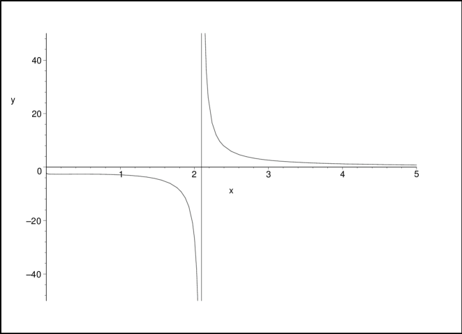
Figure 5: Behavior of the scaling dimension $\Omega_{11}$ for $\Lambda_{1}^{*}$ with respect to $x=\pi R$

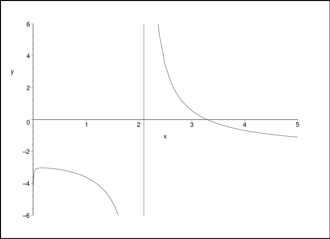
Figure 6: Behavior of the scaling dimension $\Omega_{22}$ for $\Lambda_{1}^{*}$ with respect to $x=\pi R$

These fixed points have one unstable direction. The critical coupling for such fixed points is vanishingly small ($g^{*2}\to 0,\alpha^{*}=0$) and hence the pair of $c=1$ fixed points will be infinitesimally close to the gaussian fixed point, as we have already seen in the analysis of the ungauged model [13]. As the radius is increased $\Omega_{1}$ grows to infinity as $R\to 0.70$, and $\Omega_{2}$ flips sign from negative to positive at $R=1.03$ and also grows to infinity as $R\to 0.76$. This indicates that the operator coupled to the fugacity of vortices becomes relevant at $R=1.03$ and triggers the expected liberation of the world-sheet vortices by BKT transition at the self dual radius [14, 15].

After this transition, the fixed point becomes purely repulsive up to $R\sim 0.67$. In the range $0.67\leq R\leq 0.70$, the critical coupling is infinitely large $(g^{*2}\to\infty,\alpha^{*}=0)$ as well as the scaling exponents $\Omega_{1}\to\infty,\Omega_{2}\to\infty$. As the quantity $h$ is also a large positive quantity here (figure 7), the fixed point $\Lambda_{1}^{*}$ in this region is characterized by a negative specific heat, reminiscent of Euclidean black hole in flat space-time. We will elaborate on this in the next section. These black hole like fixed points have a positive string susceptibility exponent $\gamma_{0}=(2-2/\Omega_{1})\to 2$.

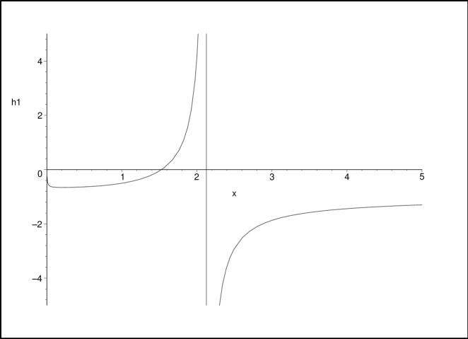
Figure 7: Behavior of $h$ for $\Lambda_{1}^{*}$ with respect to $x=\pi R$

Between $0<R\leq 0.67$ the matrix coupling $g^{*2}$, $\alpha^{*}$ and both of the scaling dimensions are negative. Hence one gets a purely attractive fixed point with imaginary matrix coupling. However, as $R\to 0$, the couplings are vanishingly small, also $h\to 0$, and one reaches a pure gravity fixed point ($c=0$) with one unstable direction as $\Omega_{1}\sim 0.8$ (such that $\gamma_{0}=2-2.5\sim-0.5$) and $\Omega_{2}\to-3.6$. Note that even though $\Lambda_{1}^{*}$ exhibits so many important features for a wide range of temperature, the constraint we have here allows us to look at it only around $R=1$ and around $R=0$. We need to improve over this constraint.

Similarly one can analyze the behavior of the fixed point $\Lambda_{2}^{*}$ with respect to the parameter $R$. It exhibits black hole like behavior ($h$ is large positive quantity) as $0\leq R\geq 0.250$. In this limit the fixed point $\Lambda_{2}^{*}(g^{*}=0,\alpha^{*}\to\infty)$ is purely repulsive, $\Omega_{1}\to\infty,\Omega_{2}\to\infty$, and hence $\gamma_{0}\to 2$ (see figure 8). However, here the constraint on the radius is $R\geq 0.19$. For the fixed points $\Lambda_{3}^{*}$, there is also similar black hole like behavior with negative specific heat at $0.51\leq R\geq 0.63$ and at $0.12\leq R\geq 0.19$ and $\gamma_{0}=2$ (see figure 9). There is no constraint on the radius.

Figure 8: Behavior of $h$ for $\Lambda_{2}^{*}$ with respect to $x=\pi R$

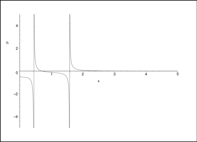
Figure 9: Behavior of $h$ for $\Lambda_{3}^{*}$ with respect to $x=\pi R$

4 Comments On The Black Hole Fixed Point

To study the thermodynamic behavior of the fixed points we would like to solve for the free energy from the Callan-Symanzik equation as one approaches the BKT phase transition (or the Hagedorn transition) and analyze its thermal properties. From the analysis of the previous section, one can see that the fixed point $\Lambda_{1}^{*}$ has rather exotic behavior around $R_{H}\sim 0.73$, little below (above) the Kosterlitz-Thouless radius (temperature) $R_{KT}=1/(2\pi T_{KT})=1$. Around this region the scaling dimensions $\Omega_{1}$, $\Omega_{2}$, and $h$, are large constants which simplifies the situation. However, as we proceed we will see that the black hole like behavior would emerge from the region where $h$ is a large positive constant. Thus around $R_{H}$ the free energy can be written as

$$\mathcal{F}_{s}\sim f[(R-R_{H}/R_{H})^{1/h},\Delta,\hat{\alpha},N]\,,$$ (4.1)

where the inverse temperatures are defined by,

$$\beta=2\pi R=\frac{1}{T}\,,~{}~{}~{}~{}\beta_{H}=2\pi R_{H}=\frac{1}{T_{H}}\,.$$ (4.2)

The thermodynamic quantities are given by

$$\mathcal{F}_{s}(\beta-\beta_{H}) = -\beta~{}F(\beta-\beta_{H})=\ln Z(\beta-\beta_{H})\,,$$

$$E = \frac{\partial(\beta F)}{\partial\beta}=\frac{-\partial\ln Z}{\partial\beta}\,,$$

$$C_{v} = -\beta^{2}\Big{(}\frac{\partial E}{\partial\beta}\Big{)}_{v}\,.$$ (4.3)

Using $\mathcal{F}_{s}$, we have

$$E \sim \frac{1}{h}~{}\beta_{H}^{-1}~{}\Big{(}\frac{\beta-\beta_{H}}{\beta_{H}}\Big{)}^{1/h-1}\,.$$

Since near the phase transition the fluctuation of energy is large, the canonical ensemble would diverge. In such situation, it is better to pass to the microcanonical ensemble with fixed energy and the temperature defined by

$$\beta=\frac{\partial S(E)}{\partial E}\,.$$ (4.5)

Using (LABEL:energy) for large positive $h$, one can solve for $\beta$ in terms of $E$ as

$$\beta-\beta_{H}\sim-\frac{h^{-1}}{E}\,.$$ (4.6)

Combining this with the definition of temperature in the microcanonical ensemble (4.5) one can calculate the near Hagedorn one loop finite energy correction to the usual definition of Hagedorn density of states, $\rho(E)=\exp[S(E)]\sim\exp[\beta_{H}E]$, and the usual inverse temperature, which is otherwise a constant $\partial S/\partial E=\beta_{H}$. The finite energy corrections are of the form

$$\beta = \frac{\partial\ln\rho}{\partial E}=\beta_{H}+\frac{s_{1}}{E}+O\bigg{(}\frac{1}{E^{2}}\bigg{)}\,,$$

$$\rho(E) \sim E^{s_{1}}~{}\exp[\beta_{H}E]\bigg{[}1+O\bigg{(}\frac{1}{E}\bigg{)}\bigg{]}\,.$$ (4.7)

Here the number $s_{1}$ would come from the one loop correction. If $s_{1}$ is negative, the specific heat is negative, i.e. increasing the energy of the system gives rise to the decrease of temperature, indicating Euclidean black hole like behavior in flat spacetime.

Integrating our equation (4.6) to get the entropy and density of states we identify the one-loop correction as

$$S(E)\sim\beta_{H}E-\frac{1}{h}\ln E\,,$$

$$\rho(E)\sim E^{-\frac{1}{h}}\exp[\beta_{H}E]\,,~{}~{}~{}s_{1}=-1/h<0\,.$$ (4.8)

This behavior is true for large positive $h$ and the corresponding range of radius only. As we have analyzed in the previous section, we encounter such fixed points $\Lambda_{1}^{*}$ of very large and positive $h$ in the region $0.67\leq R\leq 0.70$. These are pair of purely repulsive fixed points (over this region the scaling exponents $\Omega_{1},\Omega_{2}$ are also large positive constants like $h$) of large (diverging) coupling $g^{*2}\to\infty,\alpha^{*}=0$ and positive string susceptibility exponent $\gamma_{0}\sim 2$. We therefore identify such fixed points as the Euclidean Black hole like fixed points in the continuum limit, with a negative specific heat (figure 10)

$$C_{v}\sim-\frac{1}{h}~{}\frac{\beta^{2}}{(\beta-\beta_{H})^{2}}\,.$$ (4.9)

Using relations like $C_{v}=-\beta\Big{(}\frac{\partial S}{\partial\beta}\Big{)}_{v}$ the entropy as a function of temperature is

$$S(\beta-\beta_{H})\sim-\frac{1}{h}\Big{(}\log(\beta-\beta_{H})-\frac{\beta_{H}}{\beta-\beta_{H}}\Big{)}\,.$$ (4.10)

The discontinuity in entropy (a measure of the latent heat of the transition) suggest that the Hagedorn transition is a first order phase transition at little higher temperature than the KT temperature, driving the system to an unstable black hole phase.

Figure 10: Behavior of the specific heat $C_{v}$ (for $\Lambda_{1}^{*}$) with respect to $x=\pi R$

5 Discussions

In this paper, starting from a matrix quantum mechanics on a circle with a periodic boundary condition (1.1) (with gauge fields $A(t)=\Omega^{\dagger}\dot{\Omega}(t)$ as degrees of freedom apart from the matrix degrees of freedom $\phi(t)$ and also with the coupling $\alpha$ as the fugacity of vortices), we have analyzed the phase structure of the theory by a world-sheet renormalization group flow and observed following remarkable facts. The nontrivial fixed points of the flow does capture the known physics of the $2D$ string theory, namely a fixed point with the critical index of $c=1$ for large radius ($R>1$), and moreover reveals a new phase. In our previous paper [13] we have analyzed this $c=1$ fixed point in detail showing that it exhibits expected logarithmic scaling violation of the singlet free energy and the T-duality. Note that for this class of fixed point ($\Lambda_{1}^{*}$), a pair with $\alpha^{*}=0$, the vanishing $\alpha$ forces $A$ to be zero and the matrix quantum mechanics (1.1) reduces to the usual matrix quantum mechanics with periodic boundary condition studied in [13]. The flow equations also exhibit indication of phase transition at $R=1.03$ as expected in BKT phase transition undergone by the $2D$ string theory due to liberation of world-sheet vortices. However, a new phase emerges beyond the phase transition at the self-dual radius. The fixed points $\Lambda_{1}^{*}$ exhibit an unstable black hole like phase with negative specific heat, between $0.67<R<0.7$. As $R\to 0$ they end up into $c=0$ fixed points which is consistent with the expectation. For another class of fixed points $\Lambda_{3}^{*}$, a pair with both nonzero $\alpha^{*}$ and $g^{*}$, there is unstable black hole like behavior with negative specific heat above the self-dual temperature (at $0.51<R<0.63$ and at $0.12<R<0.19$). From a thermodynamic study of the free energy obtained from the Callan-Symanzik equations we show that all these unstable phases do have negative specific heat. The thermodynamic quantities indicate that the system does undergo a finite temperature phase transition around the Hagedorn temperature ($R_{H}=0.7$, around which the new phase is formed) and exhibits one loop finite energy correction to the Hagedorn density of states.

Thus the thermodynamics of the $2D$ string theory above the BKT phase transition at the self-dual radius is governed by the unstable black hole like phase with negative specific heat for a range of temperatures beyond the BKT phase transition point. The remarkable thing is that we observe phases of negative specific heat for a range of temperatures rather than at a particular temperature like the case in [17] indicating that presumably there are many black holes at temperatures other than that of $2D$ cigar black hole described by dilaton gravity. It is then meaningful to ask where do the thermal black holes that we observe end up if they evaporate? Our analysis shows one class of these unstable objects evaporate to $c=0$, the other classes end up in other black holes at higher temperatures. In $1+1$ dimension, the string theory is integrable due to infinite number of conserved charges. Thus from continuum point of view it is possible that there are other black hole solutions not only characterized by mass and temperature but also by other values of conserved charges, in which case they might be at different temperatures. Here we can mention that the understanding that the integrability of the free fermion structure perhaps prevents the formation of $c=1$ black hole is consistent from the nature of the flow and the fixed points. The $c=1$ fixed points at large $R$, dominated by the singlet sector, does not exhibit any black hole like behavior.

To actually see that these objects are black holes and to deal with the questions like the formation and the unitarity of the scattering off the black hole one needs to study the dynamics of the nonsinglet states. As the observations indicate the nonsinglet states account for the entropy of the black hole, it would be nice to realize them as the excitations of the black hole. In black hole physics it was proposed that presumably the black hole entropy is due to open string with ends lying on the event horizon. It would be really interesting to study the nonsinglet boundaries of the matrix quantum mechanics in this context. The general framework of the world-sheet renormalization group approach is useful to study these objects, which is otherwise difficult. The Hamiltonian formalism, appropriate to address the questions of black hole dynamics in the Minkowski space, is complicated due to Calogero type of interaction. However, in the renormalization group approach one can utilize the Callan-Symanzic equations to calculate the wave functions for the nonsinglet boundaries or the macroscopic loops and can construct a $S$-matrix. The wave equation for the macroscopic loops should then contain the information regarding the metric of the black hole to "see" the black hole at all. In this regard one nice observation from the renormalization group analysis is that the running of the radius with scale implies a deformation in the target space geometry if one considers the scale to go like dilaton. Presumably this could help to illuminate further the issue of getting the metric. Also it is interesting to understand the localized wave function (microscopic loop) describing the the tip of the cigar black hole [47]. The unique boundary associated to the inner core of the black hole is thought to be essential to understand the evaporation and the Hawking radiation [48]. We have work in progress on understanding the boundaries in this context.

Regarding our RG method, as we have already discussed in [13], it would be interesting to generalize the scheme for arbitrary couplings and to keep arbitrary powers of $\phi$ in the evaluation of the determinant obtained from the integration over the vector degrees of freedom ($v,v^{*}$). Here we will just mention that (as discussed in our previous papaer) because of these vectors our partition function (in the $\alpha\to 0$ limit) essentially looks like the model discussed in [45, 46] and thus is useful to understand the presence of the boundaries. As a simple step towards generalization we would like to study the flow with an additional coupling due to $\phi^{4}$ term. These might reveal finer observations and also would be helpful to test the convergence of the scheme as well. The cyclic flow structure also deserves a detail study, specially near the regime of the black hole like behavior of the nontrivial fixed points where the flow structure is complicated. We would also like to understand how the relevant operators driving our flow look like in the matrix quantum mechanics side and how they translate to the operators in the world-sheet.

Acknowledgments

We would like to thank Michael Douglas for useful discussions, comments and constant support at all stages of the work. We would also like to thank Igor Klebanov, Massimo Porrati for discussions and especially Edouard Brézin for illuminating discussions, advices and reading an early draft. We thank the organizers of the string workshop at HRI, India for hospitality during early stages of this work where part of this work was reported. The research of SD was supported in part by DOE grant DE-FG02-96ER40959. The research of TD was supported in part by NSF grants PHY-0070787 and PHY-0245068. Any opinions, findings, and conclusions or recommendations expressed in this material are those of the authors and do not necessarily reflect the views of the National Science Foundation.

Appendix

A The expression of $\Sigma[g,\alpha,\phi_{N},A_{N},R,N]$

Evaluating the diagrams, $\Sigma[g,\alpha,\phi_{N},A_{N},R,N]$ can be expressed as

$$\Sigma[g,\alpha,\phi_{N},A_{N},R,N]=1+i~{}\mbox{Tr}\bigg{[}\sum_{n}\frac{2n/R}{\frac{n^{2}}{R^{2}}+1}~{}A_{0}\bigg{]}+g~{}\mbox{Tr}\bigg{[}\sum_{n}\frac{1}{\frac{n^{2}}{R^{2}}+1}~{}\phi_{0}\bigg{]}+\alpha~{}\mbox{Tr}\bigg{[}-\sum_{k}\phi_{k}\phi_{-k}$$

$$+\sum_{m,n}\frac{(2m^{2}-5mn+2n^{2})/R^{2}}{\frac{m^{2}}{R^{2}}+1}~{}\phi_{m-n}\phi_{n-m}\bigg{]}+\frac{g^{2}}{2}~{}\mbox{Tr}\bigg{[}\sum_{m,n}\frac{1}{\big{(}\frac{m^{2}}{R^{2}}+1\big{)}\big{(}\frac{n^{2}}{R^{2}}+1\big{)}}~{}\phi_{m-n}\phi_{n-m}\bigg{]}$$

$$-\mbox{Tr}\Bigg{[}\sum_{n,k}\frac{1}{\frac{n^{2}}{R^{2}}+1}~{}A_{k}A_{-k}+\frac{1}{2!}\sum_{m,n}\frac{(m^{2}+2mn+n^{2})/R^{2}}{\big{(}\frac{m^{2}}{R^{2}}+1\big{)}\big{(}\frac{n^{2}}{R^{2}}+1\big{)}}~{}A_{m-n}A_{n-m}\Bigg{]}$$

$$+i\alpha~{}\mbox{Tr}\Bigg{[}\sum_{m,n,k}\bigg{\{}\frac{(4n-2m)/R}{\frac{m^{2}}{R^{2}}+1}-\frac{(2n-m)/R}{\frac{n^{2}}{R^{2}}+1}\bigg{\}}~{}A_{m-n-k}\phi_{k}\phi_{n-m}$$

$$+\sum_{m,n,k}\bigg{\{}\frac{(4n-2m)/R}{\frac{n^{2}}{R^{2}}+1}-\frac{(2n-m)/R}{\frac{m^{2}}{R^{2}}+1}\bigg{\}}~{}A_{m-n-k}\phi_{n-m}\phi_{k}$$

$$-\sum_{m,n,l}\frac{(2m^{2}l+4ml^{2}+m^{2}n-2l^{2}n-2m^{3}-mnl)/R^{3}}{\big{(}\frac{m^{2}}{R^{2}}+1\big{)}\big{(}\frac{l^{2}}{R^{2}}+1\big{)}}~{}A_{m-l}\phi_{l-n}\phi_{n-m}\Bigg{]}$$

$$+i\frac{g^{2}}{2}~{}\mbox{Tr}\Bigg{[}\sum_{m,n,l}\frac{(m+l)/R}{\big{(}\frac{m^{2}}{R^{2}}+1\big{)}\big{(}\frac{n^{2}}{R^{2}}+1\big{)}\big{(}\frac{l^{2}}{R^{2}}+1\big{)}}~{}A_{m-l}\phi_{l-n}\phi_{n-m}\Bigg{]}$$

$$-\frac{g^{3}}{3!}~{}\mbox{Tr}\Bigg{[}\sum_{m,n,l}\frac{1}{\big{(}\frac{m^{2}}{R^{2}}+1\big{)}\big{(}\frac{n^{2}}{R^{2}}+1\big{)}\big{(}\frac{l^{2}}{R^{2}}+1\big{)}}~{}\phi_{m-l}\phi_{l-n}\phi_{n-m}\Bigg{]}$$

$$-\alpha g~{}\mbox{Tr}\Bigg{[}\sum_{m,n,l}\frac{(4ml-2mn-2ln+n^{2})/R^{2}}{\big{(}\frac{m^{2}}{R^{2}}+1\big{)}\big{(}\frac{l^{2}}{R^{2}}+1\big{)}}~{}\phi_{m-l}\phi_{l-n}\phi_{n-m}\Bigg{]}$$

$$+\alpha~{}\mbox{Tr}\Bigg{[}\sum_{m,n,k,k^{\prime}}\bigg{\{}\frac{4}{\frac{m^{2}}{R^{2}}+1}+\frac{1}{\frac{n^{2}}{R^{2}}+1}\bigg{\}}~{}A_{m-n-k}\phi_{k}\phi_{k^{\prime}}A_{n-m-k^{\prime}}$$

$$-\sum_{m,n,k,k^{\prime}}\frac{2}{\frac{m^{2}}{R^{2}}+1}(\phi_{k}A_{m-n-k}\phi_{k^{\prime}}A_{n-m-k^{\prime}}+\phi_{k}A_{n-m-k^{\prime}}\phi_{k^{\prime}}A_{m-n-k})$$

$$-\sum_{m,n,l,k}\frac{(2m^{2}-nm+2ml-nl)/R^{2}}{\big{(}\frac{m^{2}}{R^{2}}+1\big{)}\big{(}\frac{l^{2}}{R^{2}}+1\big{)}}~{}(2A_{l-n-k}\phi_{k}\phi_{n-m}A_{m-l}-\phi_{k}A_{l-n-k}\phi_{n-m}A_{m-l})$$

$$+\sum_{m,n,l,k}\frac{(2l^{2}-nm+2ml-nl)/R^{2}}{\big{(}\frac{m^{2}}{R^{2}}+1\big{)}\big{(}\frac{l^{2}}{R^{2}}+1\big{)}}~{}(2\phi_{l-n}\phi_{k}A_{n-m-k}A_{m-l}-\phi_{l-n}A_{n-m-k}\phi_{k}A_{m-l})$$

$$+\sum_{m,n,l,k}\frac{(n^{2}-2nm+4ml-2nl)/R^{2}}{\big{(}\frac{m^{2}}{R^{2}}+1\big{)}\big{(}\frac{l^{2}}{R^{2}}+1\big{)}}~{}2\phi_{l-n}\phi_{n-m}A_{n-l-k}A_{k}\Bigg{]}$$

$$-\frac{g^{2}}{2}~{}\mbox{Tr}\Bigg{[}\sum_{m,n,l,k}\frac{1}{\big{(}\frac{m^{2}}{R^{2}}+1\big{)}\big{(}\frac{n^{2}}{R^{2}}+1\big{)}\big{(}\frac{l^{2}}{R^{2}}+1\big{)}}~{}\phi_{l-n}\phi_{n-m}A_{n-l-k}A_{k}\Bigg{]}\,.$$ (A.1)

B The Feynman Diagrams

Here we evaluate and discuss the terms in different orders of the series $\Sigma[g,\alpha,\phi_{N},A_{N},R,N]$ (A.1) using the summation rules discussed in section (3.3) and the relation (2.10) for the inverse Fourier Transform.

B.1 The terms of order O($\Phi$):

$$g~{}\mbox{Tr}\bigg{[}\sum_{n}\frac{1}{(\frac{n^{2}}{R^{2}}+1)}~{}\phi_{0}\bigg{]}=g\coth(\pi R)\int_{0}^{2\pi R}dt~{}\mbox{Tr}\Phi(t)\,.$$ (B.2)

B.2 The terms of order O($A$):

$$i~{}\mbox{Tr}\bigg{[}\sum_{n}\frac{2n/R}{(\frac{n^{2}}{R^{2}}+1)}~{}A_{0}\bigg{]}=0\,.$$ (B.3)

This is because,

$$\sum_{n}\frac{n/R}{(\frac{n^{2}}{R^{2}}+1)}=0\,.$$

B.3 The terms of order O($\Phi$$\Phi$):

$$(1) \frac{g^{2}}{2}~{}\mbox{Tr}\bigg{[}\sum_{m,n}\frac{1}{\big{(}\frac{m^{2}}{R^{2}}+1\big{)}\big{(}\frac{n^{2}}{R^{2}}+1\big{)}}~{}\phi_{m-n}\phi_{n-m}\bigg{]}$$

$$=\frac{g^{2}}{2}\int\frac{dt_{1}dt_{2}}{(2\pi R)^{2}}~{}\mbox{Tr}(\Phi(t_{1})\Phi(t_{2}))\bigg{[}\sum_{m,n}\frac{\exp\big{(}i(n-m)~{}t_{1}/R\big{)}\exp\big{(}i(m-n)~{}t_{2}/R\big{)}}{\big{(}\frac{m^{2}}{R^{2}}+1\big{)}\big{(}\frac{n^{2}}{R^{2}}+1\big{)}}\bigg{]}\,.$$

Now, changing the variables to ’center of mass’ and ’relative’ coordinates defined respectively by

$$T=\frac{t_{1}+t_{2}}{2}\,,~{}~{}~{}~{}~{}\tau=\frac{t_{1}-t_{2}}{2}\,,$$ (B.5)

we have,

$$dt_{1}~{}dt_{2}=J\Big{(}\frac{t_{1},t_{2}}{T,\tau}\Big{)}~{}dT~{}d\tau=2~{}dT~{}d\tau\,.$$ (B.6)

Hence,

$$\frac{g^{2}}{2}~{}\mbox{Tr}\bigg{[}\sum_{m,n}\frac{1}{\big{(}\frac{m^{2}}{R^{2}}+1\big{)}\big{(}\frac{n^{2}}{R^{2}}+1\big{)}}~{}\phi_{m-n}\phi_{n-m}\bigg{]}$$

$$=\frac{g^{2}}{4\pi^{2}R^{2}}\int_{0}^{2\pi R}dT\int_{-\pi R}^{\pi R}d\tau~{}\mbox{Tr}(\Phi\big{(}T+\tau)\Phi(T-\tau)\big{)}\sum_{m,n}\frac{\exp\big{(}i(n-m)~{}2\tau/R\big{)}}{\big{(}\frac{m^{2}}{R^{2}}+1\big{)}\big{(}\frac{n^{2}}{R^{2}}+1\big{)}}$$

$$\simeq\frac{g^{2}}{4\pi^{2}R^{2}}\int_{0}^{2\pi R}dT\int_{-\pi R}^{\pi R}d\tau~{}\mbox{Tr}(\Phi(T)^{2}-\tau^{2}\dot{\Phi}(T)^{2})\sum_{m,n}\frac{\exp\big{(}i(n-m)~{}2\tau/R\big{)}}{\big{(}\frac{m^{2}}{R^{2}}+1\big{)}\big{(}\frac{n^{2}}{R^{2}}+1\big{)}}$$

$$\simeq g^{2}F_{g2}(R)\int_{0}^{2\pi R}dT~{}\mbox{Tr}(\Phi(T)^{2}/2)+g^{2}\hat{F}_{g2}(R)\int_{0}^{2\pi R}dT~{}\mbox{Tr}(\dot{\Phi}(T)^{2}/2)\,,$$ (B.7)

where,

$$F_{g2}(R) = \frac{1}{2\pi^{2}R^{2}}\int_{-\pi R}^{\pi R}d\tau\sum_{m,n}\frac{\exp\big{(}i(m-n)~{}2\tau/R\big{)}}{\big{(}\frac{m^{2}}{R^{2}}+1\big{)}\big{(}\frac{n^{2}}{R^{2}}+1\big{)}}$$ (B.8)

$$= \frac{1}{2\pi^{2}R^{2}}\int_{0}^{2\pi R}d\tau^{\prime}\sum_{m,n}\frac{\exp\big{(}i(m-n)~{}\tau^{\prime}/R\big{)}}{\big{(}\frac{m^{2}}{R^{2}}+1\big{)}\big{(}\frac{n^{2}}{R^{2}}+1\big{)}}\,,~{}~{}~{}~{}(\tau^{\prime}=2\tau)$$

$$= \frac{1}{2\sinh^{2}\pi R}\int_{0}^{2\pi R}d\tau^{\prime}\cosh(\pi R+\tau^{\prime})\cosh(\pi R-\tau^{\prime})$$

$$= \frac{1}{\sinh^{2}\pi R}\bigg{[}\frac{1}{2}\pi R\cosh 2\pi R+\frac{1}{8}\sinh 4\pi R\bigg{]}\,,$$

and,

$$\hat{F}_{g2}(R) = -\frac{1}{2\pi^{2}R^{2}}\int_{-\pi R}^{\pi R}d\tau~{}\tau^{2}\sum_{m,n}\frac{\exp\big{(}i(m-n)~{}2\tau/R\big{)}}{\big{(}\frac{m^{2}}{R^{2}}+1\big{)}\big{(}\frac{n^{2}}{R^{2}}+1\big{)}}$$

$$= -\frac{1}{8\pi^{2}R^{2}}\int_{o}^{2\pi R}d\tau^{\prime}~{}\tau^{\prime 2}\sum_{m,n}\frac{\exp\big{(}i(m-n)~{}\tau^{\prime}/R\big{)}}{\big{(}\frac{m^{2}}{R^{2}}+1\big{)}\big{(}\frac{n^{2}}{R^{2}}+1\big{)}}\,,~{}~{}~{}~{}(\tau^{\prime}=2\tau)$$

$$= -\frac{1}{8\sinh^{2}\pi R}\int_{o}^{2\pi R}d\tau^{\prime}~{}\tau^{\prime 2}\cosh(\pi R+\tau)\cosh(\pi R-\tau)$$

$$= \frac{1}{\sinh^{2}\pi R}\bigg{[}\frac{1}{64}(1+8\pi^{2}R^{2})\sinh 4\pi R-\frac{\pi^{3}R^{3}}{6}\cosh 2\pi R-\frac{\pi R}{16}\cosh 4\pi R\bigg{]}\,.$$

$$(2) \alpha~{}\mbox{Tr}\bigg{[}\sum_{m,n}\frac{(2m^{2}-5mn+2n^{2})/R^{2}}{(\frac{m^{2}}{R^{2}}+1)}~{}\phi_{m-n}\phi_{n-m}\bigg{]}=\alpha\int\frac{dt_{1}dt_{2}}{(2\pi R)^{2}}~{}\mbox{Tr}(\Phi(t_{1})\Phi(t_{2}))$$

$$\bigg{[}\sum_{m,n}\frac{(2m^{2}-5mn+2n^{2})/R^{2}}{(\frac{m^{2}}{R^{2}}+1)}\exp\big{(}i(n-m)~{}t_{1}/R\big{)}\exp\big{(}i(m-n)~{}t_{2}/R\big{)}\bigg{]}$$

$$=\frac{\alpha}{2\pi^{2}R^{2}}\int_{0}^{2\pi R}dT\int_{-\pi R}^{\pi R}d\tau~{}\mbox{Tr}\big{(}\Phi(T+\tau)\Phi(T-\tau)\big{)}$$

$$\bigg{[}\sum_{m,n}\frac{(2m^{2}-5mn+2n^{2})/R^{2}}{(\frac{m^{2}}{R^{2}}+1)}\exp\big{(}i(n-m)~{}2\tau/R\big{)}\bigg{]}$$

$$\simeq\frac{\alpha}{2\pi^{2}R^{2}}\int_{0}^{2\pi R}dT\int_{-\pi R}^{\pi R}d\tau~{}\mbox{Tr}(\Phi(T)^{2}-\tau^{2}\dot{\Phi}(T)^{2})$$

$$\bigg{[}\sum_{m,n}\frac{(2m^{2}-5mn+2n^{2})/R^{2}}{(\frac{m^{2}}{R^{2}}+1)}\exp\big{(}i(n-m)~{}2\tau/R\big{)}\bigg{]}$$

Now,

$$\frac{1}{2\pi^{2}R^{2}}\int_{-\pi R}^{\pi R}d\tau\bigg{[}\sum_{m,n}\frac{(2m^{2}-5mn+2n^{2})/R^{2}}{(\frac{m^{2}}{R^{2}}+1)}\exp\big{(}i(n-m)~{}2\tau/R\big{)}\bigg{]}$$

$$=\frac{1}{4\pi^{2}R^{2}}\int_{0}^{2\pi R}d\tau^{\prime}\sum_{m,n}\frac{(2m^{2}-5mn+2n^{2})/R^{2}}{(\frac{m^{2}}{R^{2}}+1)}$$

$$\bigg{[}\exp\big{(}i(n-m)~{}\tau^{\prime}/R\big{)}+\exp\big{(}-i(n-m)~{}\tau^{\prime}/R\big{)}\bigg{]}$$

$$=\int_{0}^{2\pi R}d\tau^{\prime}\bigg{[}4\delta(-\tau^{\prime})~{}\delta(\tau^{\prime})-5\cosh\tau~{}\delta^{\prime}(\tau^{\prime})-2\coth\pi R~{}\cosh\tau~{}\delta^{\prime\prime}(\tau^{\prime})\bigg{]}\,,~{}~{}~{}(\tau^{\prime}=2\tau)$$

$$=\bigg{[}4-5~{}\lim_{\epsilon\rightarrow 0}\frac{\cosh(\epsilon)-\cosh(-\epsilon)}{2\epsilon}-2\coth\pi R~{}\lim_{\epsilon_{1}\rightarrow 0}\frac{\sinh\epsilon_{1}}{\epsilon_{1}}~{}\lim_{\epsilon_{2}\rightarrow 0}\frac{\sinh\epsilon_{2}}{\epsilon_{2}}\bigg{]}$$

$$=(4-2\coth\pi R)\,,$$

and,

$$\frac{1}{2\pi^{2}R^{2}}\int_{-\pi R}^{\pi R}d\tau~{}\tau^{2}\bigg{[}\sum_{m,n}\frac{(2m^{2}-5mn+2n^{2})/R^{2}}{(\frac{m^{2}}{R^{2}}+1)}\exp\big{(}i(n-m)~{}2\tau/R\big{)}\bigg{]}$$

$$=\frac{1}{16\pi^{2}R^{2}}\int_{0}^{2\pi R}d\tau^{\prime}~{}\tau^{\prime 2}\sum_{m,n}\frac{(2m^{2}-5mn+2n^{2})/R^{2}}{(\frac{m^{2}}{R^{2}}+1)}$$

$$\bigg{[}\exp\big{(}i(n-m)~{}\tau^{\prime}/R\big{)}+\exp\big{(}-i(n-m)~{}\tau^{\prime}/R\big{)}\bigg{]}$$

$$=\int_{0}^{2\pi R}d\tau^{\prime}\bigg{[}\tau^{\prime 2}\delta(-\tau^{\prime})~{}\delta(\tau^{\prime})-\frac{5}{8}~{}\tau^{\prime 2}\cosh\tau~{}\delta^{\prime}(\tau^{\prime})$$

$$-\frac{1}{2}\coth\pi R~{}\tau^{\prime 2}\cosh\tau~{}\delta^{\prime\prime}(\tau^{\prime})\bigg{]}\,,~{}~{}~{}(\tau^{\prime}=2\tau)$$

$$=-\bigg{[}\frac{5}{8}~{}\lim_{\epsilon\rightarrow 0}\frac{\epsilon^{2}\cosh(\epsilon)-\epsilon^{2}\cosh(-\epsilon)}{2\epsilon}$$

$$+\coth\pi R~{}\lim_{\epsilon_{1}\rightarrow 0,\epsilon_{2}\rightarrow 0}\big{(}\sinh\epsilon_{1}\sinh\epsilon_{2}+\frac{\epsilon_{1}^{2}+\epsilon_{2}^{2}}{\epsilon_{1}\epsilon_{2}}\cosh\epsilon_{1}\cosh\epsilon_{2}\big{)}\bigg{]}$$

$$=-2\coth\pi R\,.$$ (B.12)

$$(3)$$

$$-\alpha~{}\mbox{Tr}\sum_{k}\Phi_{k}\Phi_{-k}=-\frac{\alpha}{4\pi^{2}R^{2}}\int dt_{1}dt_{2}~{}\mbox{Tr}(\Phi(t_{1})\Phi(t_{2}))\sum_{k}\exp\big{(}i\frac{k}{R}(t_{1}-t_{2})\big{)}$$

$$=-\frac{\alpha}{2\pi R}\int_{0}^{2\pi R}dT~{}\mbox{Tr}\Phi(T)^{2}\,.$$

Hence, in $O(\alpha)$, the coefficients of the $O(\Phi\Phi)$ terms are given by comparing with the expression

$$\alpha~{}F_{\alpha 2}(R)\int_{0}^{2\pi R}dT~{}\mbox{Tr}(\frac{1}{2}\Phi(T)^{2})+\alpha~{}\hat{F}_{\alpha 2}\int_{0}^{2\pi R}dT~{}\mbox{Tr}(\frac{1}{2}\dot{\Phi}(T)^{2})\,,$$ (B.14)

where, after collecting all the results,

$$F_{\alpha 2}(R)=-\frac{1}{\pi R}+8-4\coth\pi R\,,~{}~{}\hat{F}_{\alpha 2}=-4\coth\pi R\,.$$ (B.15)

B.4 The terms of order O($\Phi$$\Phi$$\Phi$):

$$(1)~{} \frac{g^{2}}{6}\mbox{Tr}~{}\bigg{[}\sum_{m,n,k}\frac{1}{\big{(}\frac{m^{2}}{R^{2}}+1\big{)}\big{(}\frac{n^{2}}{R^{2}}+1\big{)}\big{(}\frac{k^{2}}{R^{2}}+1\big{)}}~{}\phi_{m-n}\phi_{n-k}\phi_{k-m}\bigg{]}$$

$$=\frac{g^{2}}{6}\int\frac{dt_{1}dt_{2}dt_{3}}{(2\pi R)^{3}}~{}\mbox{Tr}~{}(\phi(t_{1})\phi(t_{2})\phi(t_{3}))$$

$$\bigg{[}\sum_{m,n}\frac{\exp\big{(}i(n-m)~{}t_{1}/R\big{)}\exp\big{(}i(k-n)~{}t_{2}/R\big{)}\exp\big{(}i(m-k)~{}t_{1}/R\big{)}}{\big{(}\frac{m^{2}}{R^{2}}+1\big{)}\big{(}\frac{n^{2}}{R^{2}}+1\big{)}\big{(}\frac{k^{2}}{R^{2}}+1\big{)}}\bigg{]}\,.$$

Using redefinition of the variables into the "center of mass" and the "relative coordinates",

$$T=\frac{1}{3}(t_{1}+t_{2}+t_{3})\,,~{}~{}~{}\tau_{1}=(t_{1}-t_{2})\,,~{}~{}~{}~{}\tau_{2}=(t_{1}-t_{3})\,,$$

$$dt_{1}~{}dt_{2}~{}dt_{3}=J\Big{(}\frac{t_{1},t_{2},t_{3}}{T,\tau_{1},\tau_{2}}\Big{)}~{}dT~{}d\tau_{1}~{}d\tau_{2}=dT~{}d\tau_{1}~{}d\tau_{2}\,.$$

Considering $\tau_{1}$ and $\tau_{2}$ to be small and keeping the order $O(\phi^{3})$ term, above series could be evaluated as,

$$\frac{g^{3}}{6}~{}\mbox{Tr}~{}\bigg{[}\sum_{m,n,k}\frac{1}{\big{(}\frac{m^{2}}{R^{2}}+1\big{)}\big{(}\frac{n^{2}}{R^{2}}+1\big{)}\big{(}\frac{k^{2}}{R^{2}}+1\big{)}}~{}\phi_{m-n}\phi_{n-k}\phi_{k-m}\bigg{]}$$

$$=\frac{g^{3}}{48\pi^{3}R^{3}}\int_{0}^{2\pi R}dT~{}\int_{-\pi R}^{\pi R}d\tau_{1}~{}\int_{-\pi R}^{\pi R}d\tau_{2}$$

$$\mbox{Tr}\Big{(}\phi(T+\frac{\tau_{1}+\tau_{2}}{3})\phi(T-\frac{2}{3}\tau_{1}+\frac{1}{3}\tau_{2})\phi(T+\frac{1}{3}\tau_{1}-\frac{2}{3}\tau_{2})\Big{)}$$

$$\Bigg{[}\sum_{m,n,k}\frac{\exp\big{(}in\tau_{1}/R\big{)}\exp\big{(}-im\tau_{2}/R\big{)}\exp\big{(}ik(\tau_{2}-\tau_{1})/R\big{)}}{\big{(}\frac{m^{2}}{R^{2}}+1\big{)}\big{(}\frac{n^{2}}{R^{2}}+1\big{)}\big{(}\frac{k^{2}}{R^{2}}+1\big{)}}\Bigg{]}$$

$$\simeq g^{3}F_{g3}(R)\int_{0}^{2\pi R}dT~{}\mbox{Tr}(\phi(T)^{3}/3)$$ (B.17)

where,

$$F_{g3}(g,R)$$

$$=\frac{1}{16\pi^{3}R^{3}}\int_{-\pi R}^{\pi R}d\tau_{1}~{}\int_{-\pi R}^{\pi R}d\tau_{2}\Bigg{[}\sum_{m,n,k}\frac{\exp\big{(}in\tau_{1}/R\big{)}\exp\big{(}-im\tau_{2}/R\big{)}\exp\big{(}ik(\tau_{2}-\tau_{1})/R\big{)}}{\big{(}\frac{m^{2}}{R^{2}}+1\big{)}\big{(}\frac{n^{2}}{R^{2}}+1\big{)}\big{(}\frac{k^{2}}{R^{2}}+1\big{)}}\Bigg{]}$$

$$=\frac{1}{16\pi R\sinh^{2}\pi R}\int_{-\pi R}^{\pi R}d\tau_{1}~{}\int_{-\pi R}^{\pi R}d\tau_{2}~{}\cosh(\pi R-\tau_{1})~{}\cosh(\pi R+\tau_{2})$$

$$~{}\sum_{k}\frac{\exp\big{(}ik(\tau_{2}-\tau_{1})/R\big{)}}{\big{(}\frac{k^{2}}{R^{2}}+1\big{)}}$$

$$=\frac{1}{64\pi R\sinh^{2}\pi R}\int_{-2\pi R}^{2\pi R}d\hat{T}~{}\int_{-2\pi R}^{2\pi R}d\hat{\tau}~{}\big{(}\cosh(2\pi R+\hat{\tau})+\cosh\hat{\tau}\big{)}~{}\sum_{k}\frac{\exp ik\hat{\tau}/R}{\big{(}\frac{k^{2}}{R^{2}}+1\big{)}}$$

$$=\frac{\pi R}{16\sinh^{3}\pi R}\int_{0}^{2\pi R}d\hat{\tau}\Big{[}\big{(}\cosh(2\pi R+\hat{\tau})+\cosh\hat{\tau}\big{)}~{}\cosh(\pi R-\hat{\tau})$$

$$+\big{(}\cosh(2\pi R-\hat{\tau})+\cosh\hat{\tau}\big{)}~{}\cosh(\pi R+\hat{\tau})\Big{]}$$

$$=\frac{\pi R}{64\sinh^{3}\pi R(\cosh 2\pi R+\cosh 4\pi R)}~{}~{}[4\pi R\big{(}3\cosh\pi R+2\cosh 3\pi R$$

$$+2\cosh 5\pi R+\cosh 7\pi R\big{)}+\sinh\pi R+\sinh 3\pi R+\sinh 5\pi R+2\sinh 7\pi R$$

$$+\sinh 9\pi R]$$ (B.18)

$$(2)~{} -\alpha g~{}\mbox{Tr}\Bigg{[}\sum_{m,n,l}\frac{(4ml-2mn-2ln+n^{2})/R^{2}}{\big{(}\frac{m^{2}}{R^{2}}+1\big{)}\big{(}\frac{l^{2}}{R^{2}}+1\big{)}}~{}\phi_{m-l}\phi_{l-n}\phi_{n-m}\Bigg{]}$$ (B.19)

$$=-\alpha g\int\frac{dt_{1}dt_{2}dt_{3}}{(2\pi R)^{3}}~{}\mbox{Tr}~{}(\phi(t_{1})\phi(t_{2})\phi(t_{3}))\bigg{[}\sum_{m,n,l}\frac{(4ml-2mn-2ln+n^{2})/R^{2}}{\big{(}\frac{m^{2}}{R^{2}}+1\big{)}\big{(}\frac{l^{2}}{R^{2}}+1\big{)}}$$

$$\exp\big{(}-i(n-m)~{}t_{1}/R\big{)}\exp\big{(}-i(l-n)~{}t_{2}/R\big{)}\exp\big{(}-i(m-l)~{}t_{1}/R\big{)}\bigg{]}\,.$$

$$=\frac{-\alpha g}{8\pi^{3}R^{3}}\int_{0}^{2\pi R}dT~{}\int_{-\pi R}^{\pi R}d\tau_{1}~{}\int_{-\pi R}^{\pi R}d\tau_{2}$$

$$\mbox{Tr}\Big{(}\phi(T+\frac{\tau_{1}+\tau_{2}}{3})\phi(T-\frac{2}{3}\tau_{1}+\frac{1}{3}\tau_{2})\phi(T+\frac{1}{3}\tau_{1}-\frac{2}{3}\tau_{2})\Big{)}$$

$$\Bigg{[}\sum_{m,n,l}\frac{(4ml-2mn-2ln+n^{2})/R^{2}}{\big{(}\frac{m^{2}}{R^{2}}+1\big{)}\big{(}\frac{l^{2}}{R^{2}}+1\big{)}}\exp\big{(}im\tau_{1}/R\big{)}\exp\big{(}-in\tau_{2}/R\big{)}\exp\big{(}il(\tau_{2}-\tau_{1})/R\big{)}\Bigg{]}$$

$$=\frac{-\alpha g}{8\pi^{3}R^{3}}\int_{0}^{2\pi R}dT~{}\mbox{Tr}\phi(t)^{3}\int_{-\pi R}^{\pi R}d\tau_{1}~{}\int_{-\pi R}^{\pi R}d\tau_{2}\Bigg{[}\sum_{m,n,l}\frac{(4ml-2mn-2ln+n^{2})/R^{2})/R^{2}}{\big{(}\frac{m^{2}}{R^{2}}+1\big{)}\big{(}\frac{l^{2}}{R^{2}}+1\big{)}}$$

$$\exp\big{(}im\tau_{1}/R\big{)}\exp\big{(}-in\tau_{2}/R\big{)}\exp\big{(}il(\tau_{2}-\tau_{1})/R\big{)}\Bigg{]}$$

Now,

$$\frac{-4\alpha g}{8\pi^{3}R^{3}}\int_{-\pi R}^{\pi R}d\tau_{1}~{}\int_{-\pi R}^{\pi R}d\tau_{2}\Bigg{[}\sum_{m,n,l}\frac{ml/R^{2}}{\big{(}\frac{m^{2}}{R^{2}}+1\big{)}\big{(}\frac{l^{2}}{R^{2}}+1\big{)}}$$

$$\exp\big{(}im\tau_{1}/R\big{)}\exp\big{(}-in\tau_{2}/R\big{)}\exp\big{(}il(\tau_{2}-\tau_{1})/R\big{)}\Bigg{]}$$

$$=\frac{-4\alpha g}{8\pi^{3}R^{3}}\int_{-\pi R}^{\pi R}d\tau_{1}~{}\int_{-\pi R}^{\pi R}d\tau_{2}~{}2\pi R\delta(t_{2})~{}\sum_{m,n,l}\frac{ml/R^{2}}{\big{(}\frac{m^{2}}{R^{2}}+1\big{)}\big{(}\frac{l^{2}}{R^{2}}+1\big{)}}$$

$$\Bigg{[}\exp\big{(}im\tau_{1}/R\big{)}\exp\big{(}il(\tau_{2}-\tau_{1})/R\big{)}+\exp\big{(}-im\tau_{1}/R\big{)}\exp\big{(}il(\tau_{2}+\tau_{1})/R\big{)}$$

$$\exp\big{(}im\tau_{1}/R\big{)}\exp\big{(}-il(\tau_{2}+\tau_{1})/R\big{)}+\exp\big{(}-im\tau_{1}/R\big{)}\exp\big{(}-il(\tau_{2}-\tau_{1})/R\big{)}\Bigg{]}$$

$$=\frac{2\alpha g}{\sinh^{2}\pi R}\Big{[}\pi R\cosh 2\pi R-\sinh\pi R/2\Big{]}\,.$$ (B.20)

Also,

$$\frac{-\alpha g}{8\pi^{3}R^{3}}\int_{-\pi R}^{\pi R}d\tau_{1}~{}\int_{-\pi R}^{\pi R}d\tau_{2}\Bigg{[}\sum_{m,n,l}\frac{n/R^{2}}{\big{(}\frac{m^{2}}{R^{2}}+1\big{)}\big{(}\frac{l^{2}}{R^{2}}+1\big{)}}$$

$$\exp\big{(}im\tau_{1}/R\big{)}\exp\big{(}-in\tau_{2}/R\big{)}\exp\big{(}il(\tau_{2}-\tau_{1})/R\big{)}\Bigg{]}$$

$$=\frac{-\alpha g}{8\pi^{3}R^{3}}\int_{-\pi R}^{\pi R}d\tau_{1}~{}\int_{-\pi R}^{\pi R}d\tau_{2}~{}\Bigg{[}-2\pi R\delta^{\prime\prime}(\tau_{2})\sum_{m,l}\frac{1}{\big{(}\frac{m^{2}}{R^{2}}+1\big{)}\big{(}\frac{l^{2}}{R^{2}}+1\big{)}}$$

$$\exp\big{(}im\tau_{1}/R\big{)}\exp\big{(}il(\tau_{2}-\tau_{1})/R\big{)}+\exp\big{(}-im\tau_{1}/R\big{)}\exp\big{(}il(\tau_{2}+\tau_{1})/R\big{)}$$

$$-2\pi R\delta^{\prime\prime}(-\tau_{2})\sum_{m,l}\frac{1}{\big{(}\frac{m^{2}}{R^{2}}+1\big{)}\big{(}\frac{l^{2}}{R^{2}}+1\big{)}}\exp\big{(}im\tau_{1}/R\big{)}\exp\big{(}-il(\tau_{2}+\tau_{1})/R\big{)}$$

$$+\exp\big{(}-im\tau_{1}/R\big{)}\exp\big{(}-il(\tau_{2}-\tau_{1})/R\big{)}\Bigg{]}$$

$$=\frac{\alpha g}{4\sinh^{2}\pi R}\int_{-\pi R}^{\pi R}d\tau_{1}\cosh(\pi R+\tau_{1})\cosh(\pi R-\tau_{1})$$

$$\lim_{\epsilon\to 0,\delta\to 0}\big{(}(\cosh(\epsilon+\delta)-\cosh(\epsilon-\delta))/\epsilon\delta\big{)}$$

$$=\frac{\alpha g}{4\sinh^{2}\pi R}\Big{[}\pi R\cosh 2\pi R+\sinh\pi R/2\Big{]}\,.$$ (B.21)

The last but one term can be evaluated as,

$$\frac{-2\alpha g}{8\pi^{3}R^{3}}\int_{-\pi R}^{\pi R}d\tau_{1}~{}\int_{-\pi R}^{\pi R}d\tau_{2}\Bigg{[}\sum_{m,n,l}\frac{mn/R^{2}}{\big{(}\frac{m^{2}}{R^{2}}+1\big{)}\big{(}\frac{l^{2}}{R^{2}}+1\big{)}}$$

$$\exp\big{(}im\tau_{1}/R\big{)}\exp\big{(}-in\tau_{2}/R\big{)}\exp\big{(}il(\tau_{2}-\tau_{1})/R\big{)}\Bigg{]}$$

$$=\frac{-2\alpha g}{8\pi^{3}R^{3}}\int_{-\pi R}^{\pi R}d\tau_{1}~{}\int_{-\pi R}^{\pi R}d\tau_{2}~{}\Bigg{[}-2\pi R\delta^{\prime}(\tau_{2})\sum_{m,l}\frac{1}{\big{(}\frac{m^{2}}{R^{2}}+1\big{)}\big{(}\frac{l^{2}}{R^{2}}+1\big{)}}$$

$$\exp\big{(}im\tau_{1}/R\big{)}\exp\big{(}il(\tau_{2}-\tau_{1})/R\big{)}+\exp\big{(}-im\tau_{1}/R\big{)}\exp\big{(}il(\tau_{2}+\tau_{1})/R\big{)}$$

$$-2\pi R\delta^{\prime}(-\tau_{2})\sum_{m,l}\frac{1}{\big{(}\frac{m^{2}}{R^{2}}+1\big{)}\big{(}\frac{l^{2}}{R^{2}}+1\big{)}}\exp\big{(}im\tau_{1}/R\big{)}\exp\big{(}-il(\tau_{2}+\tau_{1})/R\big{)}$$

$$+\exp\big{(}-im\tau_{1}/R\big{)}\exp\big{(}-il(\tau_{2}-\tau_{1})/R\big{)}\Bigg{]}$$

$$=\frac{\alpha g}{\sinh^{2}\pi R}\int_{-\pi R}^{\pi R}d\tau_{1}\sinh(\pi R+\tau_{1})\sinh(\pi R-\tau_{1})\lim_{\epsilon\to 0}\sinh\epsilon/\epsilon$$

$$=\frac{\alpha g}{2\sinh^{2}\pi R}\Big{[}\pi R\cosh 2\pi R-\sinh\pi R/2\Big{]}\,.$$ (B.22)

Thus combining all the terms,

$$-\alpha g~{}\mbox{Tr}\Bigg{[}\sum_{m,n,l}\frac{(4ml-2mn-2ln+n^{2})/R^{2}}{\big{(}\frac{m^{2}}{R^{2}}+1\big{)}\big{(}\frac{l^{2}}{R^{2}}+1\big{)}}~{}\phi_{m-l}\phi_{l-n}\phi_{n-m}\Bigg{]}=F_{\alpha g3}\alpha g\int_{0}^{2\pi R}dt\mbox{Tr}\phi^{2}(t)/3\,,$$ (B.23)

where,

$$F_{\alpha g3}=(\frac{13}{4}\frac{\pi R}{\sinh^{2}\pi R}\cosh\pi R-\frac{11}{4}\frac{\sinh 2\pi R}{2})\,.$$ (B.24)

B.5 The terms of order O($A$$A$):

(1)

$$-\mbox{Tr}\Bigg{[}\sum_{n,k}\frac{1}{\frac{n^{2}}{R^{2}}+1}~{}A_{k}A_{-k}\Bigg{]}=\frac{1}{2}\coth\pi R\int_{0}^{2\pi R}dt~{}\mbox{Tr}(A^{2}(t))$$ (B.25)

$$(2) -\mbox{Tr}\Bigg{[}\frac{1}{2!}\sum_{m,n}\frac{(m^{2}+2mn+n^{2})/R^{2}}{\big{(}\frac{m^{2}}{R^{2}}+1\big{)}\big{(}\frac{n^{2}}{R^{2}}+1\big{)}}~{}A_{m-n}A_{n-m}\Bigg{]}$$ (B.26)

$$=-\frac{1}{8\pi^{2}R^{2}}\int_{0}^{2\pi R}~{}dt_{1}~{}dt_{2}\mbox{Tr}(A(t_{1})A(t_{2}))~{}\sum_{m,n}\frac{(m^{2}+2mn+n^{2})/R^{2}}{\big{(}\frac{m^{2}}{R^{2}}+1\big{)}\big{(}\frac{n^{2}}{R^{2}}+1\big{)}}~{}\exp(im(t_{2}-t_{1})/R)$$

$$~{}\exp(in(t_{1}-t_{2})/R)$$

$$\simeq-\frac{1}{4\pi^{2}R^{2}}\int_{0}^{2\pi R}~{}dT~{}\mbox{Tr}(A^{2}(T))~{}\int_{0}^{\pi R}d\tau~{}\sum_{m,n}\frac{(m^{2}+2mn+n^{2})/R^{2}}{\big{(}\frac{m^{2}}{R^{2}}+1\big{)}\big{(}\frac{n^{2}}{R^{2}}+1\big{)}}$$

$$\big{(}\exp(i2m\tau/R)~{}\exp(-i2n\tau/R)+$$

$$\exp(-i2m\tau/R)~{}\exp(i2n\tau/R)+\exp(i2m\tau/R)~{}\exp(i2n\tau/R)+\exp(-i2m\tau/R)~{}\exp(-i2n\tau/R)\big{)}$$

$$=-4\coth\pi R~{}\int_{0}^{2\pi R}~{}dT~{}\mbox{Tr}(A^{2}(T))-\frac{1}{2\sinh^{2}\pi R}~{}\int_{0}^{\pi R}d\tau\big{(}2\sinh(\pi R-\tau)\sinh(\pi R+\tau)+$$

$$\sinh(\pi R-\tau)\sinh(\pi R-\tau)+\sinh(\pi R+\tau)\sinh(\pi R+\tau)\big{)}~{}\int_{0}^{2\pi R}~{}dT~{}\mbox{Tr}(A^{2}(T))$$

$$=-\Big{(}4\coth\pi R+\frac{1}{2}~{}\pi R~{}(1+\coth^{2}\pi R)-\frac{1}{2}\coth\pi R-\frac{\pi R}{2\sinh^{2}\pi R}\Big{)}~{}\int_{0}^{2\pi R}~{}dT~{}\mbox{Tr}(A^{2}(T))$$

Hence, the terms of O($A$$A$) are given by,

$$G_{2}(R)\int dt~{}\mbox{Tr}A^{2}(t)\,,$$ (B.27)

where,

$$G_{2}(R)=(-3\coth\pi R-\frac{1}{2}~{}\pi R~{}(1+\coth^{2}\pi R)+\frac{\pi R}{2\sinh^{2}\pi R})\,.$$ (B.28)

B.6 The terms of order O($A$$\Phi$$\Phi$):

$$(1) i\frac{g^{2}}{2}~{}\mbox{Tr}\Bigg{[}\sum_{m,n,l}\frac{(m+l)/R}{\big{(}\frac{m^{2}}{R^{2}}+1\big{)}\big{(}\frac{n^{2}}{R^{2}}+1\big{)}\big{(}\frac{l^{2}}{R^{2}}+1\big{)}}~{}A_{m-l}\phi_{l-n}\phi_{n-m}\Bigg{]}$$

$$=i\frac{g^{2}}{2}\int\frac{dt_{1}dt_{2}dt_{3}}{(2\pi R)^{3}}~{}\mbox{Tr}\big{(}A(t_{1})\Phi(t_{2})\Phi(t_{3})\big{)}$$

$$\Bigg{[}\sum_{m,n,l}\frac{(m+l)/R}{\big{(}\frac{m^{2}}{R^{2}}+1\big{)}\big{(}\frac{n^{2}}{R^{2}}+1\big{)}\big{(}\frac{l^{2}}{R^{2}}+1\big{)}}$$

$$\exp\big{(}il(t_{1}-t_{2})/R\big{)}\exp\big{(}in(t_{2}-t_{3})/R\big{)}\exp\big{(}im(t_{3}-t_{1})/R\big{)}\Bigg{]}$$

Now we will use the following redefinition of the variables into the "center of mass" and "relative coordinates",

$$T=\frac{1}{3}(t_{1}+t_{2}+t_{3})\,,~{}~{}~{}\tau_{1}=(t_{1}-t_{2})\,,~{}~{}~{}~{}\tau_{2}=(t_{1}-t_{3})\,,$$

$$dt_{1}~{}dt_{2}~{}dt_{3}=J\Big{(}\frac{t_{1},t_{2},t_{3}}{T,\tau_{1},\tau_{2}}\Big{)}~{}dT~{}d\tau_{1}~{}d\tau_{2}=dT~{}d\tau_{1}~{}d\tau_{2}\,.$$

Considering $\tau_{1}$ and $\tau_{2}$ to be small and neglecting the terms of the order $O(A(t)\Phi(t)^{2})$, $O(A(t)\dot{\Phi}(t)^{2})$, $O(A(t)\dot{\Phi}(t)\Phi(t))$, and $O(A(t)\Phi(t)\dot{\Phi}(t))$, and keeping terms of the form $O(A(t)[\Phi(t),\dot{\Phi}(t)])$ only, above series could be evaluated as,

$$i\frac{g^{2}}{2}~{}\mbox{Tr}\Bigg{[}\sum_{m,n,l}\frac{(m+l)/R}{\big{(}\frac{m^{2}}{R^{2}}+1\big{)}\big{(}\frac{n^{2}}{R^{2}}+1\big{)}\big{(}\frac{l^{2}}{R^{2}}+1\big{)}}~{}A_{m-l}\phi_{l-n}\phi_{n-m}\Bigg{]}$$

$$=i\frac{g^{2}}{8\pi^{3}R^{3}}\int_{0}^{2\pi R}dT~{}\int_{-\pi R}^{\pi R}d\tau_{1}~{}\int_{-\pi R}^{\pi R}d\tau_{2}~{}\mbox{Tr}\Big{(}A(T+\frac{\tau_{1}+\tau_{2}}{3})\Phi(T-\frac{2}{3}\tau_{1}+\frac{1}{3}\tau_{2})\Phi(T+\frac{1}{3}\tau_{1}-\frac{2}{3}\tau_{2})\Big{)}$$

$$\Bigg{[}\sum_{m,n,l}\frac{(m+l)/R}{\big{(}\frac{m^{2}}{R^{2}}+1\big{)}\big{(}\frac{n^{2}}{R^{2}}+1\big{)}\big{(}\frac{l^{2}}{R^{2}}+1\big{)}}\exp\big{(}il\tau_{1}/R\big{)}\exp\big{(}-im\tau_{2}/R\big{)}\exp\big{(}in(\tau_{2}-\tau_{1})/R\big{)}\Bigg{]}$$

$$\simeq i\frac{g^{2}}{8\pi^{3}R^{3}}\int_{0}^{2\pi R}dT~{}\mbox{Tr}A(T)\big{[}\Phi(T),\dot{\Phi}(T\big{]}\int_{-\pi R}^{\pi R}d\tau_{1}~{}\int_{-\pi R}^{\pi R}d\tau_{2}\big{(}\frac{\tau_{1}-\tau_{2}}{3}\big{)}$$

$$\Bigg{[}\sum_{m,n,l}\frac{(m+l)/R}{\big{(}\frac{m^{2}}{R^{2}}+1\big{)}\big{(}\frac{n^{2}}{R^{2}}+1\big{)}\big{(}\frac{l^{2}}{R^{2}}+1\big{)}}\exp\big{(}il\tau_{1}/R\big{)}\exp\big{(}-im\tau_{2}/R\big{)}\exp\big{(}in(\tau_{2}-\tau_{1})/R\big{)}\Bigg{]}$$

$$=\frac{g^{2}}{12}\big{(}\pi R\cosh 2\pi R-\frac{1}{2}\sinh 2\pi R\big{)}\,,$$ (B.30)

Where,

$$\int_{-\pi R}^{\pi R}d\tau_{1}~{}\int_{-\pi R}^{\pi R}d\tau_{2}\big{(}\frac{\tau_{1}-\tau_{2}}{3}\big{)}\Bigg{[}\sum_{m,n,l}\frac{(m+l)/R}{\big{(}\frac{m^{2}}{R^{2}}+1\big{)}\big{(}\frac{n^{2}}{R^{2}}+1\big{)}\big{(}\frac{l^{2}}{R^{2}}+1\big{)}}$$

$$\exp\big{(}i\frac{l\tau_{1}}{R}\big{)}\exp\big{(}-i\frac{m\tau_{2}}{R}\big{)}\exp\big{(}i\frac{n(\tau_{2}-\tau_{1})}{R}\big{)}\Bigg{]}$$

$$=\frac{1}{3}\int_{0}^{\pi R}d\tau_{1}\int_{0}^{\pi R}d\tau_{2}\sum_{m,n,l}\frac{(m+l)/R}{\big{(}\frac{m^{2}}{R^{2}}+1\big{)}\big{(}\frac{n^{2}}{R^{2}}+1\big{)}\big{(}\frac{l^{2}}{R^{2}}+1\big{)}}\Bigg{[}(\tau_{1}-\tau_{2})\Big{\{}\exp\big{(}i\frac{l\tau_{1}}{R}\big{)}\exp\big{(}-i\frac{m\tau_{2}}{R}\big{)}$$

$$\exp\big{(}i\frac{n(\tau_{2}-\tau_{1})}{R}\big{)}-\exp\big{(}-i\frac{l\tau_{1}}{R}\big{)}\exp\big{(}i\frac{m\tau_{2}}{R}\big{)}\exp\big{(}-i\frac{n(\tau_{2}-\tau_{1})}{R}\big{)}\Big{\}}+(\tau_{1}+\tau_{2})\Big{\{}\exp\big{(}i\frac{l\tau_{1}}{R}\big{)}$$

$$\exp\big{(}i\frac{m\tau_{2}}{R}\big{)}\exp\big{(}-i\frac{n(\tau_{2}+\tau_{1})}{R}\big{)}-\exp\big{(}-i\frac{l\tau_{1}}{R}\big{)}\exp\big{(}-i\frac{m\tau_{2}}{R}\big{)}\exp\big{(}i\frac{n(\tau_{2}+\tau_{1})}{R}\big{)}\Big{\}}\Bigg{]}$$

$$=-i\frac{2}{3}\frac{\pi^{3}R^{3}\cosh\pi R}{\sinh^{3}\pi R}\int_{0}^{\pi R}d\tau_{1}\int_{0}^{\pi R}d\tau_{2}\Big{(}\tau_{1}\sinh 2\tau_{1}\cosh 2\tau_{2}-\tau_{2}\sinh 2\tau_{2}\cosh 2\tau_{1}\Big{)}$$

$$=-i\frac{2}{3}\pi^{3}R^{3}\coth^{2}\pi R\big{(}\pi R\cosh 2\pi R-\frac{1}{2}\sinh 2\pi R\big{)}\,.$$ (B.31)

$$(2) -i\alpha~{}\mbox{Tr}\Bigg{[}\sum_{m,n,l}\frac{(2m^{2}l+4ml^{2}+m^{2}n-2l^{2}n-2m^{3}-mnl)/R^{3}}{\big{(}\frac{m^{2}}{R^{2}}+1\big{)}\big{(}\frac{l^{2}}{R^{2}}+1\big{)}}~{}A_{m-l}\phi_{l-n}\phi_{n-m}\Bigg{]}$$

$$=-i\alpha\int\frac{dt_{1}dt_{2}dt_{3}}{(2\pi R)^{3}}~{}\mbox{Tr}\big{(}A(t_{1})\Phi(t_{2})\Phi(t_{3})\big{)}\Bigg{[}\sum_{m,n,l}\frac{(2m^{2}l+4ml^{2}+m^{2}n-2l^{2}n-2m^{3}-mnl)/R^{3}}{\big{(}\frac{m^{2}}{R^{2}}+1\big{)}\big{(}\frac{l^{2}}{R^{2}}+1\big{)}}$$

$$\exp\big{(}il(t_{1}-t_{2})/R\big{)}\exp\big{(}in(t_{2}-t_{3})/R\big{)}\exp\big{(}im(t_{3}-t_{1})/R\big{)}\Bigg{]}$$

$$=-\frac{i\alpha}{8\pi^{3}R^{3}}\int_{0}^{2\pi R}dT~{}\int_{-\pi R}^{\pi R}d\tau_{1}~{}\int_{-\pi R}^{\pi R}d\tau_{2}~{}\mbox{Tr}\Big{(}A(T+\frac{\tau_{1}+\tau_{2}}{3})\Phi(T-\frac{2}{3}\tau_{1}+\frac{1}{3}\tau_{2})\Phi(T+\frac{1}{3}\tau_{1}-\frac{2}{3}\tau_{2})\Big{)}$$

$$\Bigg{[}\sum_{m,n,l}\frac{(2m^{2}l+4ml^{2}+m^{2}n-2l^{2}n-2m^{3}-mnl)/R^{3}}{\big{(}\frac{m^{2}}{R^{2}}+1\big{)}\big{(}\frac{l^{2}}{R^{2}}+1\big{)}}\exp\big{(}i\frac{l\tau_{1}}{R}\big{)}\exp\big{(}-i\frac{m\tau_{2}}{R}\big{)}\exp\big{(}i\frac{n(\tau_{2}-\tau_{1})}{R}\big{)}\Bigg{]}$$

$$\simeq-\frac{i\alpha}{8\pi^{3}R^{3}}\int_{0}^{2\pi R}dT~{}\mbox{Tr}A(T)\big{[}\Phi(T),\dot{\Phi}(T\big{]}~{}\int_{-\pi R}^{\pi R}d\tau_{1}~{}\int_{-\pi R}^{\pi R}d\tau_{2}\big{(}\frac{\tau_{1}-\tau_{2}}{3}\big{)}$$

$$\Bigg{[}\sum_{m,n,l}\frac{(2m^{2}l+4ml^{2}+m^{2}n-2l^{2}n-2m^{3}-mnl)/R^{3}}{\big{(}\frac{m^{2}}{R^{2}}+1\big{)}\big{(}\frac{l^{2}}{R^{2}}+1\big{)}}\exp\big{(}i\frac{l\tau_{1}}{R}\big{)}\exp\big{(}-i\frac{m\tau_{2}}{R}\big{)}\exp\big{(}i\frac{n(\tau_{2}-\tau_{1})}{R}\big{)}\Bigg{]}$$

Now contribution of the different terms on the above sum can be evaluated as,

$$(2.a)~{} -\frac{i\alpha}{24\pi^{3}R^{3}}~{}\int_{-\pi R}^{\pi R}d\tau_{1}~{}\int_{-\pi R}^{\pi R}d\tau_{2}\big{(}\tau_{1}-\tau_{2}\big{)}\Bigg{[}\sum_{m,n,l}\frac{(2m^{2}l+4ml^{2})/R^{3}}{\big{(}\frac{m^{2}}{R^{2}}+1\big{)}\big{(}\frac{l^{2}}{R^{2}}+1\big{)}}\exp\big{(}i\frac{l\tau_{1}}{R}\big{)}$$ (B.33)

$$\exp\big{(}-i\frac{m\tau_{2}}{R}\big{)}\exp\big{(}i\frac{n}{R}(\tau_{2}-\tau_{1})\big{)}\Bigg{]}$$

$$=-i\frac{4\alpha}{3}\int_{0}^{\pi R}d\tau_{1}~{}\tau_{1}~{}\delta(\tau_{1})\sum_{l}\frac{l/R~{}\sinh l\tau_{1}/R}{((l^{2}/R^{2})+1)}$$

$$=0\,.$$

$$(2.b)~{} -\frac{i\alpha}{24\pi^{3}R^{3}}~{}\int_{-\pi R}^{\pi R}d\tau_{1}~{}\int_{-\pi R}^{\pi R}d\tau_{2}\big{(}\tau_{1}-\tau_{2}\big{)}\Bigg{[}\sum_{m,n,l}\frac{(2m^{2}n-2l^{2}n)/R^{3}}{\big{(}\frac{m^{2}}{R^{2}}+1\big{)}\big{(}\frac{l^{2}}{R^{2}}+1\big{)}}\exp\big{(}i\frac{l\tau_{1}}{R}\big{)}$$ (B.34)

$$\exp\big{(}-i\frac{m\tau_{2}}{R}\big{)}\exp\big{(}i\frac{n}{R}(\tau_{2}-\tau_{1})\big{)}\Bigg{]}$$

$$=\frac{-i\alpha}{24\pi^{3}R^{3}}\int_{0}^{\pi R}d\tau_{1}\int_{0}^{\pi R}d\tau_{2}\sum_{m,n,l}\frac{m^{2}n/R^{3}}{\big{(}\frac{m^{2}}{R^{2}}+1\big{)}\big{(}\frac{l^{2}}{R^{2}}+1\big{)}}\Bigg{[}(\tau_{1}-\tau_{2})\Big{\{}\exp\big{(}in(\tau_{2}-\tau_{1})/R\big{)}$$

$$\Big{(}\exp\big{(}il\tau_{1}/R\big{)}\exp\big{(}-im\tau_{2}/R\big{)}-2\exp\big{(}im\tau_{1}/R\big{)}\exp\big{(}-il\tau_{2}/R\big{)}\Big{)}$$

$$-\exp\big{(}-in(\tau_{2}-\tau_{1})/R\big{)}\Big{(}\exp\big{(}-il\tau_{1}/R\big{)}\exp\big{(}im\tau_{2}/R\big{)}-2\exp\big{(}-im\tau_{1}/R\big{)}\exp\big{(}il\tau_{2}/R\big{)}\Big{)}\Big{\}}$$

$$+(\tau_{1}+\tau_{2})\Big{\{}\exp\big{(}-in(\tau_{2}+\tau_{1})/R\big{)}\Big{(}\exp\big{(}il\tau_{1}/R\big{)}\exp\big{(}im\tau_{2}/R\big{)}-2\exp\big{(}im\tau_{1}/R\big{)}\exp\big{(}il\tau_{2}/R\big{)}\Big{)}$$

$$-\exp\big{(}in(\tau_{2}+\tau_{1})/R\big{)}\Big{(}\exp\big{(}-il\tau_{1}/R\big{)}\exp\big{(}-im\tau_{2}/R\big{)}-2\exp\big{(}-im\tau_{1}/R\big{)}\exp\big{(}-il\tau_{2}/R\big{)}\Big{)}\Big{\}}\Bigg{]}$$

$$=\frac{\alpha}{3\pi R}\int_{0}^{\pi R}d\tau_{1}~{}\tau_{1}~{}\Big{(}\delta^{\prime}(-\tau_{1})\sum_{l}\frac{\exp(il\tau_{1}/R)}{(l^{2}/R^{2})+1}-\delta^{\prime}(\tau_{1})\sum_{l}\frac{\exp(-il\tau_{1}/R)}{(l^{2}/R^{2})+1}\Big{)}$$

$$=-\frac{2}{3}\alpha\coth\pi R\,.$$

$$(2.c)~{} -\frac{i\alpha}{12\pi^{3}R^{3}}~{}\int_{-\pi R}^{\pi R}d\tau_{1}~{}\int_{-\pi R}^{\pi R}d\tau_{2}\big{(}\tau_{1}-\tau_{2}\big{)}\Bigg{[}\sum_{m,n,l}\frac{m^{3}/R^{3}}{\big{(}\frac{m^{2}}{R^{2}}+1\big{)}\big{(}\frac{l^{2}}{R^{2}}+1\big{)}}\exp\big{(}i\frac{l\tau_{1}}{R}\big{)}\exp\big{(}-i\frac{m\tau_{2}}{R}\big{)}$$ (B.35)

$$\exp\big{(}i\frac{n}{R}(\tau_{2}-\tau_{1})\big{)}\Bigg{]}$$

$$=\frac{-i\alpha}{12\pi^{3}R^{3}}\int_{0}^{\pi R}d\tau_{1}\int_{0}^{\pi R}d\tau_{2}\sum_{m,n,l}\frac{m^{3}/R^{3}}{\big{(}\frac{m^{2}}{R^{2}}+1\big{)}\big{(}\frac{l^{2}}{R^{2}}+1\big{)}}\Bigg{[}(\tau_{1}-\tau_{2})\Big{\{}\exp\big{(}in(\tau_{2}-\tau_{1})/R\big{)}\exp\big{(}il\tau_{1}/R\big{)}$$

$$\exp\big{(}-im\tau_{2}/R\big{)}-\exp\big{(}-in(\tau_{2}-\tau_{1})\exp\big{(}im\tau_{2}/R\big{)}\exp\big{(}-il\tau_{1}/R\big{)}\Big{\}}$$

$$+(\tau_{1}+\tau_{2})\Big{\{}\exp\big{(}il\tau_{1}/R\big{)}\exp\big{(}im\tau_{2}/R\big{)}\exp\big{(}-in(\tau_{2}+\tau_{1})/R\big{)}$$

$$-\exp\big{(}-im\tau_{2}/R\big{)}\exp\big{(}-il\tau_{1}/R\big{)}\exp\big{(}in(\tau_{2}+\tau_{1})/R\big{)}\Big{\}}\Bigg{]}$$

$$=\frac{-\alpha}{3\pi R}\sum_{l}\frac{1}{\frac{l^{2}}{R^{2}}+1}\int_{0}^{\pi R}d\tau_{1}\int_{0}^{\pi R}d\tau_{2}\Big{[}(\tau_{1}-\tau_{2})\Big{(}\delta(\tau_{2}-\tau_{1})\delta^{\prime}(-\tau_{2})\exp\big{(}il\tau_{1}/R\big{)}-\delta(-\tau_{2}+\tau_{1})\delta^{\prime}(\tau_{2})$$

$$\exp\big{(}-il\tau_{1}/R\big{)}\Big{)}+(\tau_{1}+\tau_{2})\Big{(}\delta(-\tau_{1}-\tau_{2})\delta^{\prime}(\tau_{2})\exp\big{(}il\tau_{1}/R\big{)}$$

$$-\delta(\tau_{1}+\tau_{2})\delta^{\prime}(-\tau_{2})\exp\big{(}-il\tau_{1}/R\big{)}\Big{)}\Big{]}=0$$

$$(2.d)~{} -\frac{i\alpha}{24\pi^{3}R^{3}}~{}\int_{-\pi R}^{\pi R}d\tau_{1}~{}\int_{-\pi R}^{\pi R}d\tau_{2}\big{(}\tau_{1}-\tau_{2}\big{)}\Bigg{[}\sum_{m,n,l}\frac{mnl/R^{3}}{\big{(}\frac{m^{2}}{R^{2}}+1\big{)}\big{(}\frac{l^{2}}{R^{2}}+1\big{)}}\exp\big{(}i\frac{l\tau_{1}}{R}\big{)}\exp\big{(}-i\frac{m\tau_{2}}{R}\big{)}$$ (B.36)

$$\exp\big{(}i\frac{n}{R}(\tau_{2}-\tau_{1})\big{)}\Bigg{]}$$

$$=\frac{-i\alpha}{24\pi^{3}R^{3}}\int_{0}^{\pi R}d\tau_{1}\int_{0}^{\pi R}d\tau_{2}\sum_{m,n,l}\frac{mnl/R^{3}}{\big{(}\frac{m^{2}}{R^{2}}+1\big{)}\big{(}\frac{l^{2}}{R^{2}}+1\big{)}}\Bigg{[}(\tau_{1}-\tau_{2})\Big{\{}\exp\big{(}il\tau_{1}/R\big{)}\exp\big{(}-im\tau_{2}/R\big{)}$$

$$\exp\big{(}in(\tau_{2}-\tau_{1})/R\big{)}-\exp\big{(}im\tau_{2}/R\big{)}\exp\big{(}-il\tau_{1}/R\big{)}\exp\big{(}-in(\tau_{2}-\tau_{1})/R\big{)}\Big{\}}$$

$$+(\tau_{1}+\tau_{2})\Big{\{}\exp\big{(}il\tau_{1}/R\big{)}\exp\big{(}im\tau_{2}/R\big{)}\exp\big{(}-in(\tau_{2}+\tau_{1})/R\big{)}$$

$$-\exp\big{(}-im\tau_{2}/R\big{)}\exp\big{(}-il\tau_{1}/R\big{)}\exp\big{(}in(\tau_{2}+\tau_{1})/R\big{)}\Big{\}}\Bigg{]}$$

$$=\frac{\alpha}{24\sinh^{2}\pi R}\int_{0}^{\pi R}d\tau_{1}\int_{0}^{\pi R}d\tau_{2}~{}\Big{[}(\tau_{1}-\tau_{2})\Big{(}\delta^{\prime}(\tau_{2}-\tau_{1})(\cosh(2\pi R+\tau_{2}-\tau_{1})-\cosh(\tau_{2}+\tau_{1}))$$

$$-\delta^{\prime}(\tau_{1}-\tau_{2})(\cosh(2\pi R+\tau_{1}-\tau_{2})-\cosh(\tau_{1}+\tau_{2}))\Big{)}$$

$$+(\tau_{1}+\tau_{2})\Big{(}\delta^{\prime}(-\tau_{2}-\tau_{1})(\cosh(2\pi R-\tau_{2}-\tau_{1})-\cosh(\tau_{2}-\tau_{1}))-$$

$$\delta^{\prime}(\tau_{1}+\tau_{2})(\cosh(2\pi R+\tau_{1}+\tau_{2})-\cosh(\tau_{2}-\tau_{1}))\Big{)}\Big{]}$$

$$=-\frac{\alpha}{\sinh^{2}\pi R}\Big{(}\frac{\pi R}{6}\cosh\pi R+\frac{1}{12}\sinh\pi R\Big{)}$$

(3)

$$i\alpha~{}\mbox{Tr}\sum_{m,n,k}\bigg{\{}\frac{(4n-2m)/R}{\frac{m^{2}}{R^{2}}+1}-\frac{(2n-m)/R}{\frac{n^{2}}{R^{2}}+1}\bigg{\}}~{}A_{m-n-k}\phi_{k}\phi_{n-m}$$

$$=\frac{i\alpha}{8\pi^{3}R^{3}}\int_{0}^{2\pi R}dt_{1}~{}dt_{2}~{}dt_{3}~{}\mbox{Tr}(A(t_{1})\phi(t_{2})\phi(t_{3}))\sum_{m,n,k}\bigg{\{}\frac{(4n-2m)/R}{\frac{m^{2}}{R^{2}}+1}-\frac{(2n-m)/R}{\frac{n^{2}}{R^{2}}+1}\bigg{\}}$$

$$\exp(ik(t_{1}-t_{2})/R)~{}\exp(im(t_{3}-t_{1})/R)~{}\exp(in(t_{1}-t_{3})/R)$$

$$=\frac{i\alpha}{24\pi^{3}R^{3}}\int_{0}^{2\pi R}dT~{}\mbox{Tr}(A(T)[\phi(T),\phi(\dot{T})])~{}\int_{-\pi R}^{\pi R}~{}d\tau_{1}~{}d\tau_{2}~{}(\tau_{1}-\tau_{2})\sum_{m,n,k}\bigg{\{}\frac{(4n-2m)/R}{\frac{m^{2}}{R^{2}}+1}-\frac{(2n-m)/R}{\frac{n^{2}}{R^{2}}+1}\bigg{\}}$$

$$\exp(ik(\tau_{2}-\tau_{1})/R)~{}\exp(im\tau_{1}/R)~{}\exp(-in\tau_{1}/R)$$

$$=0\,.$$ (B.37)

As the overall behavior of the function is proportional to $\int_{-\pi R}^{\pi R}~{}d\tau_{1}~{}d\tau_{2}~{}(\tau_{1}-\tau_{2})\delta(\tau_{1}-\tau_{2})$ , therefore the contribution vanishes. Similarly the contribution of the other term with similar sum

$$i\alpha~{}\sum_{m,n,k}\bigg{\{}\frac{(4n-2m)/R}{\frac{n^{2}}{R^{2}}+1}-\frac{(2n-m)/R}{\frac{m^{2}}{R^{2}}+1}\bigg{\}}~{}A_{m-n-k}\phi_{n-m}\phi_{k}$$ (B.38)

vanishes also. Thus, the O$(A[\phi,\dot{\phi}])$ term is given by

$$(G_{g3}~{}g^{2}+G_{\alpha 3}~{}\alpha)\int dt~{}A(t)[\phi(t),\dot{\phi}(t)]\,,$$

where,

$$G_{g3}(R)=\frac{1}{12}(\pi R\cosh 2\pi R-\frac{1}{2}\sinh 2\pi R)$$

$$G_{\alpha 3}(R)=-\frac{2}{3}\coth\pi R-\frac{1}{\sinh^{2}\pi R}(\frac{\pi R}{6}\cosh\pi R+\frac{1}{12}\sinh\pi R)\,.$$ (B.39)

B.7 The terms of order O($A^{2}\Phi^{2}$)

$$(1).~{} 2\alpha~{}\mbox{Tr}~{}\Bigg{[}\sum_{m,n,l,k}\frac{(n^{2}-2nm+4ml-2nl)/R^{2}}{\big{(}\frac{m^{2}}{R^{2}}+1\big{)}\big{(}\frac{l^{2}}{R^{2}}+1\big{)}}~{}2\phi_{l-n}\phi_{n-m}A_{m-l-k}A_{k}\Bigg{]}$$

$$=\frac{2\alpha}{(2\pi R)^{4}}\int_{0}^{2\pi R}dt_{1}~{}dt_{2}~{}dt_{3}~{}dt_{4}~{}\mbox{Tr}\big{(}A(t_{1})\phi(t_{2})\phi(t_{3})A(t_{4})\big{)}\sum_{m,n,l,k}\frac{(n^{2}-2nm+4ml-2nl)/R^{2}}{\big{(}\frac{m^{2}}{R^{2}}+1\big{)}\big{(}\frac{l^{2}}{R^{2}}+1\big{)}}$$

$$\exp(i\frac{k}{R}(t_{3}-t_{4}))~{}\exp(i\frac{l}{R}(t_{3}-t_{1}))~{}\exp(i\frac{n}{R}(t_{1}-t_{2}))~{}\exp(i\frac{m}{R}(t_{2}-t_{3}))~{}$$

Again using the usual redefinition of the variables into the "center of mass" and "relative coordinates",

$$T=\frac{1}{4}(t_{1}+t_{2}+t_{3}+t_{4})\,,~{}~{}~{}\tau_{1}=(t_{4}-t_{1})\,,~{}~{}~{}~{}\tau_{2}=(t_{4}-t_{2})~{}~{}~{}~{}\tau_{3}=(t_{4}-t_{3})\,,$$

$$dt_{1}~{}dt_{2}~{}dt_{3}~{}dt_{4}=J\Big{(}\frac{t_{1},t_{2},t_{3},t_{4}}{T,\tau_{1},\tau_{2},\tau_{3}}\Big{)}~{}dT~{}d\tau_{1}~{}d\tau_{2}~{}d\tau_{3}=dT~{}d\tau_{1}~{}d\tau_{2}~{}d\tau_{3}\,.$$

Considering $\tau_{1}$, $\tau_{2}$ and $\tau_{4}$ to be small and keeping terms of the form $O(A(t)^{2}\Phi(t)^{2})$ only, above series could be evaluated as,

$$2\alpha~{}\mbox{Tr}~{}\Bigg{[}\sum_{m,n,l,k}\frac{(n^{2}-2nm+4ml-2nl)/R^{2}}{\big{(}\frac{m^{2}}{R^{2}}+1\big{)}\big{(}\frac{l^{2}}{R^{2}}+1\big{)}}~{}2\phi_{l-n}\phi_{n-m}A_{m-l-k}A_{k}\Bigg{]}$$

$$\simeq\frac{2\alpha}{(2\pi R)^{3}}\int_{-\pi R}^{\pi R}~{}d\tau_{1}~{}d\tau_{2}~{}\sum_{m,n,l}\frac{(n^{2}-2nm+4ml-2nl)/R^{2}}{\big{(}\frac{m^{2}}{R^{2}}+1\big{)}\big{(}\frac{l^{2}}{R^{2}}+1\big{)}}~{}\exp(i\frac{l}{R}(\tau_{1}))~{}$$

$$\exp(i\frac{n}{R}(\tau_{2}-\tau_{1}))~{}\exp(-i\frac{m}{R}(\tau_{2}))~{}\int_{0}^{2\pi R}dT~{}\mbox{Tr}\Big{(}\phi^{2}(T)A^{2}(T)\Big{)}$$

$$=\frac{4\alpha}{(2\pi R)^{3}}\int_{0}^{2\pi R}dT~{}\mbox{Tr}\Big{(}\phi^{2}(T)A^{2}(T)\Big{)}\sum_{m,n,l}\frac{(n^{2}-2nm+4ml-2nl)/R^{2}}{\big{(}\frac{m^{2}}{R^{2}}+1\big{)}\big{(}\frac{l^{2}}{R^{2}}+1\big{)}}$$

$$\int_{-\pi R}^{\pi R}~{}d\hat{\tau}_{1}~{}d\hat{\tau}_{2}~{}\exp(i\frac{l}{R}(\hat{\tau}_{1}+\hat{\tau}_{2}))~{}\exp(-i\frac{n}{R}2\hat{\tau}_{2})~{}\exp(i\frac{m}{R}(\hat{\tau}_{2}-\hat{\tau}_{1}))~{}$$

The terms containing powers of $n$ in the numerator of the sum inserts higher and higher derivatives of delta function over time variables and are eventually computed to be zero. The only non-vanishing contribution comes from the term without $n$ in the numerator.

$$\frac{4~{}\alpha}{(2\pi R)^{3}}\int_{0}^{2\pi R}dT~{}\mbox{Tr}\Big{(}\phi^{2}(T)A^{2}(T)\Big{)}\sum_{m,n,l}\frac{4ml/R^{2}}{\big{(}\frac{m^{2}}{R^{2}}+1\big{)}\big{(}\frac{l^{2}}{R^{2}}+1\big{)}}$$

$$\int_{0}^{\pi R}~{}d\hat{\tau}_{1}~{}d\hat{\tau}_{2}~{}\Big{(}\exp(i\frac{l}{R}(\hat{\tau}_{1}+\hat{\tau}_{2}))~{}\exp(-i\frac{n}{R}2\hat{\tau}_{2})~{}\exp(i\frac{m}{R}(\hat{\tau}_{2}-\hat{\tau}_{1}))$$

$$+\exp(i\frac{l}{R}(\hat{\tau}_{1}-\hat{\tau}_{2}))~{}\exp(i\frac{n}{R}(2\hat{\tau}_{2}))~{}\exp(-i\frac{m}{R}(\hat{\tau}_{2}+\hat{\tau}_{1}))+\exp(-i\frac{l}{R}(\hat{\tau}_{1}-\hat{\tau}_{2}))$$

$$~{}\exp(i\frac{n}{R}(-2\hat{\tau}_{2}))~{}\exp(i\frac{m}{R}(\hat{\tau}_{2}+\hat{\tau}_{1}))+~{}\exp(-i\frac{l}{R}(\hat{\tau}_{1}+\hat{\tau}_{2}))~{}\exp(i\frac{n}{R}(2\hat{\tau}_{2})~{}\exp(-i\frac{m}{R}(\hat{\tau}_{2}-\hat{\tau}_{1}))\Big{)}$$

$$=-\frac{16~{}\alpha}{\sinh^{2}\pi R}\int_{0}^{2\pi R}dT~{}\mbox{Tr}\Big{(}\phi^{2}(T)A^{2}(T)\Big{)}\int_{0}^{\pi R}d\hat{\tau}_{1}\Big{(}\sinh(\pi R-\hat{\tau}_{1})\sinh(\pi R+\hat{\tau}_{1})\Big{)}$$

$$=-\frac{8~{}\alpha}{\sinh^{2}\pi R}(\pi R\cosh 2\pi R-\frac{1}{2}\sinh 2\pi R)\int_{0}^{2\pi R}dT~{}\mbox{Tr}\Big{(}\phi^{2}(T)A^{2}(T)\Big{)}$$ (B.42)

(2)  Similarly,

$$-2~{}\alpha~{}\mbox{Tr}\Bigg{[}\sum_{m,n,l,k}\frac{(2m^{2}-nm+2ml-nl)/R^{2}}{\big{(}\frac{m^{2}}{R^{2}}+1\big{)}\big{(}\frac{l^{2}}{R^{2}}+1\big{)}}~{}(\phi_{n-m}A_{m-l}A_{l-n-k}\phi_{k})\Bigg{]}$$

$$=\frac{2~{}\alpha}{(2\pi R)^{4}}\int_{0}^{2\pi R}dt_{1}~{}dt_{2}~{}dt_{3}~{}dt_{4}~{}\mbox{Tr}\big{(}\phi(t_{1})A(t_{2})A(t_{3})\phi(t_{4})\big{)}\sum_{m,n,l,k}\frac{(2m^{2}-nm+2ml-nl)/R^{2}}{\big{(}\frac{m^{2}}{R^{2}}+1\big{)}\big{(}\frac{l^{2}}{R^{2}}+1\big{)}}$$

$$\exp(i\frac{k}{R}(t_{3}-t_{4}))~{}\exp(i\frac{l}{R}(t_{2}-t_{3}))~{}\exp(i\frac{n}{R}(t_{3}-t_{1}))~{}\exp(i\frac{m}{R}(t_{1}-t_{2}))~{}$$

$$\simeq\frac{2~{}\alpha}{(2\pi R)^{3}}\int_{0}^{2\pi R}dT~{}\mbox{Tr}\big{(}\phi(T)A(T)A(T)\phi(T)\big{)}\int_{-\pi R}^{\pi R}d\tau_{1}d\tau_{2}\sum_{m,n,l,k}\frac{(2m^{2}-nm+2ml-nl)/R^{2}}{\big{(}\frac{m^{2}}{R^{2}}+1\big{)}\big{(}\frac{l^{2}}{R^{2}}+1\big{)}}$$

$$\exp(-i\frac{l}{R}\tau_{2})~{}\exp(i\frac{n}{R}\tau_{1})~{}\exp(i\frac{m}{R}(\tau_{2}-\tau_{1}))~{}$$

$$\simeq\alpha\big{(}\frac{5}{2}\coth\pi R-2\pi R(1+\coth^{2}\pi R)\big{)}~{}\int_{0}^{2\pi R}dT~{}\mbox{Tr}\big{(}\phi(T)A(T)A(T)\phi(T)\big{)}$$ (B.43)

In evaluating above expression again we see that the term containing (any power of) $n$ in the numerator of the sum is not contributing. Again,

$$2~{}\alpha~{}\mbox{Tr}\Bigg{[}\sum_{m,n,l,k}\frac{(2l^{2}-nm+2ml-nl)/R^{2}}{\big{(}\frac{m^{2}}{R^{2}}+1\big{)}\big{(}\frac{l^{2}}{R^{2}}+1\big{)}}~{}(A_{m-l}\phi_{l-n}\phi_{k}A_{n-m-k})\Bigg{]}$$

$$=\frac{2~{}\alpha}{(2\pi R)^{4}}\int_{0}^{2\pi R}dt_{1}~{}dt_{2}~{}dt_{3}~{}dt_{4}~{}\mbox{Tr}\big{(}A(t_{1})\phi(t_{2})\phi(t_{3})A(t_{4})\big{)}\sum_{m,n,l,k}\frac{(2l^{2}-nm+2ml-nl)/R^{2}}{\big{(}\frac{2m^{2}}{R^{2}}+1\big{)}\big{(}\frac{l^{2}}{R^{2}}+1\big{)}}$$

$$\exp(i\frac{k}{R}(t_{4}-t_{3}))~{}\exp(i\frac{l}{R}(t_{1}-t_{2}))~{}\exp(i\frac{n}{R}(t_{2}-t_{4}))~{}\exp(i\frac{m}{R}(t_{4}-t_{1}))~{}$$

$$\simeq\frac{2~{}\alpha}{(2\pi R)^{3}}\int_{0}^{2\pi R}dT~{}\mbox{Tr}\big{(}A(T)\phi(T)\phi(T)A(T)\big{)}\int_{-\pi R}^{\pi R}d\tau_{1}d\tau_{2}\sum_{m,n,l,k}\frac{(2l^{2}-nm+2ml-nl)/R^{2}}{\big{(}\frac{m^{2}}{R^{2}}+1\big{)}\big{(}\frac{l^{2}}{R^{2}}+1\big{)}}$$

$$\exp(i\frac{m}{R}\tau_{1})~{}\exp(-i\frac{n}{R}\tau_{2})~{}\exp(i\frac{l}{R}(\tau_{2}-\tau_{1}))\,.$$

Exchanging $l\leftrightarrow m$ and $\tau_{1}\leftrightarrow-\tau_{2}$, this gives equal and opposite contribution to the previous expression and hence all the similar pair of sums

$$-\alpha\sum_{m,n,l,k}\frac{(2m^{2}-nm+2ml-nl)/R^{2}}{\big{(}\frac{m^{2}}{R^{2}}+1\big{)}\big{(}\frac{l^{2}}{R^{2}}+1\big{)}}~{}(2A_{l-n-k}\phi_{k}\phi_{n-m}A_{m-l}-\phi_{k}A_{l-n-k}\phi_{n-m}A_{m-l})$$

$$+\alpha\sum_{m,n,l,k}\frac{(2l^{2}-nm+2ml-nl)/R^{2}}{\big{(}\frac{m^{2}}{R^{2}}+1\big{)}\big{(}\frac{l^{2}}{R^{2}}+1\big{)}}~{}(2\phi_{l-n}\phi_{k}A_{n-m-k}A_{m-l}-\phi_{l-n}A_{n-m-k}\phi_{k}A_{m-l})\,,$$

give zero contribution.

$$(3)~{} \alpha~{}\mbox{Tr}\Bigg{[}\sum_{m,n,k,k^{\prime}}\bigg{\{}\frac{4}{\frac{m^{2}}{R^{2}}+1}+\frac{1}{\frac{n^{2}}{R^{2}}+1}\bigg{\}}~{}A_{m-n-k}\phi_{k}\phi_{k^{\prime}}A_{n-m-k^{\prime}}\Bigg{]}$$ (B.46)

$$=\frac{\alpha}{(2\pi R)^{4}}\int_{0}^{2\pi R}dt_{1}~{}dt_{2}~{}dt_{3}~{}dt_{4}~{}\mbox{Tr}\big{(}A(t_{1})\phi(t_{2})\phi(t_{3})A(t_{4})\big{)}\sum_{m,n,k,k^{\prime}}\Big{(}\frac{4}{\frac{m^{2}}{R^{2}}+1}+\frac{1}{\frac{n^{2}}{R^{2}}+1}\Big{)}$$

$$\exp(i\frac{k}{R}(t_{1}-t_{2}))~{}\exp(i\frac{k^{\prime}}{R}(t_{4}-t_{3}))~{}\exp(i\frac{n}{R}(t_{1}-t_{4}))~{}\exp(i\frac{m}{R}(t_{4}-t_{1}))~{}$$

$$\simeq\frac{5\alpha}{2}\coth\pi R\int_{0}^{2\pi R}dT~{}\mbox{Tr}\big{(}A(T)\phi(T)\phi(T)A(T)\big{)}$$

(4)  Similraly,

$$-\alpha~{}\mbox{Tr}\Big{[}\sum_{m,n,k,k^{\prime}}\frac{2}{\frac{m^{2}}{R^{2}}+1}\big{(}\phi_{k}A_{m-n-k}\phi_{k^{\prime}}A_{n-m-k^{\prime}}+\phi_{k}A_{n-m-k^{\prime}}\phi_{k^{\prime}}A_{m-n-k}\big{)}\Big{]}$$

$$=\frac{-\alpha}{(2\pi R)^{4}}\int_{0}^{2\pi R}dt_{1}~{}dt_{2}~{}dt_{3}~{}dt_{4}~{}\mbox{Tr}\big{(}A(t_{1})\phi(t_{2})A(t_{3})\phi(t_{4})\big{)}\sum_{m,n,k,k^{\prime}}\Big{(}\frac{2}{\frac{n^{2}}{R^{2}}+1}\Big{)}$$

$$\Big{\{}\exp(i\frac{k}{R}(t_{2}-t_{1}))~{}\exp(i\frac{k^{\prime}}{R}(t_{4}-t_{3}))~{}\exp(i\frac{n}{R}(t_{2}-t_{4}))~{}\exp(i\frac{m}{R}(t_{4}-t_{2}))~{}$$

$$+\exp(i\frac{k}{R}(t_{4}-t_{1}))~{}\exp(i\frac{k^{\prime}}{R}(t_{2}-t_{3}))~{}\exp(i\frac{n}{R}(t_{4}-t_{2}))~{}\exp(i\frac{m}{R}(t_{2}-t_{4}))\Big{\}}$$

$$\simeq-2\alpha\coth\pi R\int_{0}^{2\pi R}dT~{}\mbox{Tr}\big{(}A(T)\phi(T)A(T)\phi(T)\big{)}$$ (B.47)

(5)

$$-\frac{g^{2}}{2}~{}\mbox{Tr}\Big{[}\sum_{m,n,l,k}\frac{1}{\big{(}\frac{m^{2}}{R^{2}}+1\big{)}\big{(}\frac{n^{2}}{R^{2}}+1\big{)}\big{(}\frac{l^{2}}{R^{2}}+1\big{)}}~{}\phi_{l-n}\phi_{n-m}A_{m-l-k}A_{k}\Big{]}$$

$$=-\frac{g^{2}}{2(2\pi R)^{4}}~{}\int_{0}^{2\pi R}dt_{1}~{}dt_{2}~{}dt_{3}~{}dt_{4}~{}\mbox{Tr}\big{(}A(t_{1})\phi(t_{2})A(t_{3})\phi(t_{4})\big{)}\sum_{m,n,l,k}\frac{1}{\big{(}\frac{m^{2}}{R^{2}}+1\big{)}\big{(}\frac{n^{2}}{R^{2}}+1\big{)}\big{(}\frac{l^{2}}{R^{2}}+1\big{)}}$$

$$\exp(i\frac{k}{R}(t_{3}-t_{4}))~{}\exp(i\frac{l}{R}(t_{3}-t_{1}))~{}\exp(i\frac{n}{R}(t_{1}-t_{2}))~{}\exp(i\frac{m}{R}(t_{2}-t_{3}))~{}$$

$$\simeq-\frac{g^{2}}{16(\pi R)^{3}}\int_{0}^{2\pi R}dT~{}\mbox{Tr}\big{(}A(T)\phi(T)A(T)\phi(T)\big{)}~{}\sum_{m,n,l,}\frac{1}{\big{(}\frac{m^{2}}{R^{2}}+1\big{)}\big{(}\frac{n^{2}}{R^{2}}+1\big{)}\big{(}\frac{l^{2}}{R^{2}}+1\big{)}}$$

$$\int_{-\pi R}^{\pi R}d\tau_{1}d\tau_{2}~{}\exp(-i\frac{l}{R}\tau_{2})~{}\exp(i\frac{n}{R}\tau_{1})~{}\exp(i\frac{m}{R}(\tau_{2}-\tau_{1}))~{}\,,$$

where,

$$-\frac{g^{2}}{16(\pi R)^{3}}~{}\sum_{m,n,l,}\frac{1}{\big{(}\frac{m^{2}}{R^{2}}+1\big{)}\big{(}\frac{n^{2}}{R^{2}}+1\big{)}\big{(}\frac{l^{2}}{R^{2}}+1\big{)}}\int_{-\pi R}^{\pi R}d\tau_{1}d\tau_{2}~{}\exp(-i\frac{l}{R}\tau_{2})~{}\exp(i\frac{n}{R}\tau_{1})~{}\exp(i\frac{m}{R}(\tau_{2}-\tau_{1}))$$

$$=-\frac{g^{2}}{8\pi R\sinh\pi R}~{}\sum_{m}\frac{1}{\big{(}\frac{m^{2}}{R^{2}}+1\big{)}}\int_{0}^{\pi R}d\tau_{1}d\tau_{2}~{}\big{(}\sinh(\pi R+\tau_{2})\sinh(\pi R-\tau_{1})\exp(i\frac{m}{R}(\tau_{2}-\tau_{1}))+$$

$$\sinh(\pi R+\tau_{2})\sinh(\pi R+\tau_{1})\exp(i\frac{m}{R}(\tau_{2}+\tau_{1}))\big{)}$$

$$=-\frac{g^{2}}{16\pi R\sinh\pi R}~{}\sum_{m}\frac{1}{\big{(}\frac{m^{2}}{R^{2}}+1\big{)}}\int_{0}^{\pi R}d\tau_{1}d\tau_{2}~{}\Big{(}\big{(}\cosh(2\pi R+\tau_{2}-\tau_{1})-\cosh(\tau_{1}+\tau_{2})\big{)}$$

$$\exp(i\frac{m}{R}(\tau_{2}-\tau_{1}))+$$

$$\big{(}\cosh(2\pi R+\tau_{1}+\tau_{2})-\cosh(\tau_{1}-\tau_{2})\big{)}\exp(i\frac{m}{R}(\tau_{2}+\tau_{1}))\Big{)}$$

$$=-\frac{g^{2}}{8\pi R\sinh\pi R}~{}\sum_{m}\frac{1}{\big{(}\frac{m^{2}}{R^{2}}+1\big{)}}\int_{0}^{\pi R}d\hat{T}~{}\int_{-\pi R/2}^{\pi R/2}d\hat{\tau}~{}\Big{(}\big{(}\cosh(2\pi R+2\hat{\tau})-\cosh(2T)\big{)}\exp(i\frac{2m}{R}\hat{\tau})+$$

$$\big{(}\cosh(2\pi R+2T)-\cosh(2\hat{\tau})\big{)}\exp(i\frac{2m}{R}T)\Big{)}$$

$$=-\frac{g^{2}}{8\pi R\sinh\pi R}~{}\Big{[}\int_{-\pi R/2}^{\pi R/2}d\hat{\tau}~{}\big{(}\pi R~{}\cosh(2\pi R+2\hat{\tau})-\frac{1}{2}\sinh(2\pi R)\big{)}\sum_{m}\frac{1}{\big{(}\frac{m^{2}}{R^{2}}+1\big{)}}~{}\exp(i\frac{2m}{R}\hat{\tau})+$$

$$\int_{0}^{\pi R}dT~{}\big{(}\pi R\cos h(2\pi R+2T)-\sinh(\pi R)\big{)}~{}\frac{\pi R}{\sinh\pi R}\cosh(\pi R-2T)\Big{]}$$

$$=-\frac{g^{2}}{8\sinh^{2}\pi R}~{}\int_{0}^{\pi R}dT\Big{[}~{}\big{(}\frac{\pi R}{2}~{}\cosh(2\pi R+T)-\frac{1}{4}\sinh 2\pi R\big{)}\cosh(\pi R-T)+\big{(}\frac{\pi R}{2}~{}\cosh(2\pi R-T)$$

$$-\frac{1}{4}\sinh 2\pi R\big{)}\cosh(\pi R+T)+\big{(}\pi R\cosh(2\pi R+2T)-\sinh(\pi R)\big{)}~{}\cosh(\pi R-2T)\Big{]}$$

$$=-\frac{g^{2}}{8\sinh^{2}\pi R}\Big{(}\pi^{2}R^{2}\cosh 3\pi R+\frac{\pi R}{8}\sinh 5\pi R+\frac{\pi R}{4}\sinh 3\pi R$$

$$-\frac{3}{8}\sinh\pi R+\frac{1}{4}\sinh^{2}2\pi R-\sinh^{2}\pi R\Big{)}$$

Collecting all the terms, the O$(A\phi A\phi)$ and the O$(\phi^{2}A^{2})$ terms are given by

$$(G_{g4}g^{2}+G_{\alpha 4}\alpha\int dt~{}\mbox{Tr}A(t)\phi(t)A(t)\phi(t)+(G^{\prime}_{g4}g^{2}+G^{\prime}_{\alpha 4}\alpha)\int dt~{}\mbox{Tr}A^{2}(t)\phi^{2}(t)\,,$$

where,

$$G_{g4}(R)=-\frac{1}{8\sinh^{2}\pi R}\Big{(}\pi^{2}R^{2}\cosh 3\pi R+\frac{\pi R}{8}\sinh 5\pi R+\frac{\pi R}{4}\sinh 3\pi R-\frac{3}{8}\sinh\pi R$$

$$+\frac{1}{4}\sinh^{2}2\pi R-\sinh^{2}\pi R\Big{)}$$

$$G^{\prime}_{g4}(R)=0$$

$$G_{\alpha 4}(R)=-2\coth\pi R$$

$$G^{\prime}_{\alpha 4}(R)=\frac{5}{2}\coth\pi R\,.$$ (B.50)

C The Scaling Dimensions

For $\Lambda^{*}_{1}$,

$$\Omega_{11}=\frac{4F_{g3}+3F_{g2}+3F_{g1}+\frac{3}{2}G_{g4}}{\hat{F}_{g2}-F_{g1}-F_{g2}-3G_{g4}-2F_{g3}}\,,$$

$$\Omega_{12}=\frac{3\hat{F}_{\alpha 2}+2F_{\alpha g3}}{\hat{F}_{g2}-F_{g1}-F_{g2}-3G_{g4}-2F_{g3}}\,,$$

$$\Omega_{21}=0\,,$$

$$\Omega_{22}=-2\Big{(}\frac{\hat{F}_{g2}+F_{g2}+F_{g1}-2G_{g3}+\frac{3}{2}G_{g4}+F_{g3}}{\hat{F}_{g2}-F_{g1}-F_{g2}-3G_{g4}-2F_{g3}}\Big{)}\,.$$ (C.51)

For $\Lambda^{*}_{2}$,

$$\Omega_{11}=\frac{6F_{\alpha g3}+6F_{\alpha 2}+3G_{\alpha 4}-2G_{2}}{\hat{F}_{\alpha 2}-F_{\alpha 2}-3G_{\alpha 4}+2G_{2}-2F_{\alpha g3}}\,,$$

$$\Omega_{12}=0\,,$$

$$\Omega_{21}=0\,,$$

$$\Omega_{22}=\frac{6\hat{F}_{\alpha 2}+2F_{\alpha 2}-8G_{\alpha 3}+3G_{\alpha 4}+2G_{2}+2F_{\alpha g3}}{\hat{F}_{\alpha 2}-F_{\alpha 2}-3G_{\alpha 4}+2G_{2}-2F_{\alpha g3}}\,.$$ (C.52)

References

- [1] D.J. Gross and N. Miljkovic, ‘‘A Nonperturbative Solution of D = 1 String Theory’’, Phys. Lett. B238, 217 (1990).
- [2] E. Brezin, V.A. Kazakov, and A. B. Zamolodchikov, ‘‘Scaling Violation in a Field Theory of Closed Strings in One Dimension’’, Nucl. Phys. B338, 673 (1990).
- [3] P. Ginsparg and J. Zinn-Justin, ‘‘2-D Gravity 1-D Matter’’, Phys. Lett. B240, 333 (1990).
- [4] G. Parisi, ‘‘On the One-Dimensional Discretized String’’, Phys. Lett. B238, 209 (1990).
- [5] J. McGreevy and H. verlinde, ‘‘Strings from Tachyons: the c=1 Matrix Reloaded’’; hep-th/0304224.
- [6] E.J. Martinec, ‘‘The Annular Report on Non-Critical String Theory’’; hep-th/0305148.
- [7] I.R. Klebanov, J. Maldacena and N. Seiberg, ‘‘D-brane Decay in Two-Dimensional String Theory, JHEP 0307, 045 (2003).
- [8] J. McGreevy, J. Teschner and H. Verlinde, ‘‘Classical and Quantum D-branes in 2D String Theory’’; hep-th/0305194.
- [9] S.Yu. Alexandrov, V.A. Kazakov and D. Kutasov, ‘‘Non-Perturbative Effects in Matrix Models and D-branes’’; hep-th/0306177.
- [10] T. Takayanagi and N. Toumbas, ‘‘A matrix model dual of type 0B string theory in two dimensions,’’ JHEP 0307, 064 (2003) hep-th/0307083.
- [11] M. R. Douglas, I. R. Klebanov, D. Kutasov, J. Maldacena, E. Martinec and N. Seiberg, ‘‘A new hat for the c = 1 matrix model,’’ hep-th/0307195.
- [12] A. Sen, ‘‘Open-Closed Duality: Lessons from the Matrix Model’’; hep-th/0308068.
- [13] S. Dasgupta and T. Dasgupta, ‘‘Renormalization group approach to c = 1 matrix model on a circle and D-brane decay,’’ hep-th/0310106.
- [14] D. J. Gross and I. R. Klebanov, ‘‘One-Dimensional String Theory On A Circle,’’ Nucl. Phys. B 344, 475 (1990).
- [15] D. J. Gross and I. R. Klebanov, ‘‘Vortices And The Nonsinglet Sector Of The C = 1 Matrix Model,’’ Nucl. Phys. B 354, 459 (1991).
- [16] D. Boulatov and V. Kazakov, ‘‘One-dimensional string theory with vortices as the upside down matrix oscillator,’’ Int. J. Mod. Phys. A 8, 809 (1993); hep-th/0012228.
- [17] V. Kazakov, I. K. Kostov and D. Kutasov, ‘‘A matrix model for the two-dimensional black hole,’’ Nucl. Phys. B 622, 141 (2002); hep-th/0101011.
- [18] S. Elitzur, A. Forge and E. Rabinovici, ‘‘Some Global Aspects Of String Compactifications,’’ Nucl. Phys. B 359, 581 (1991).
- [19] G. Mandal, A. M. Sengupta and S. R. Wadia, ‘‘Classical solutions of two-dimensional string theory,’’ Mod. Phys. Lett. A 6, 1685 (1991).
- [20] E. Witten, ‘‘On string theory and black holes,’’ Phys. Rev. D 44, 314 (1991).
- [21] A. Dhar, G. Mandal and S. R. Wadia, ‘‘Stringy quantum effects in two-dimensional black hole,’’ Mod. Phys. Lett. A 7, 3703 (1992); hep-th/9210120.
- [22] J. G. Russo, ‘‘Black hole formation in c = 1 string field theory,’’ Phys. Lett. B 300, 336 (1993); hep-th/9211057.
- [23] T. Yoneya, ‘‘Matrix models and 2-D critical string theory: 2-D black hole by c = 1 matrix model,’’ hep-th/9211079.
- [24] S. R. Das, ‘‘Matrix Models And Nonperturbative String Propagation In Two-Dimensional Black Hole Backgrounds,’’ Mod. Phys. Lett. A 8, 1331 (1993); hep-th/9303116.
- [25] A. Dhar, G. Mandal and S. R. Wadia, ‘‘Wave propagation in stringy black hole,’’ Mod. Phys. Lett. A 8, 1701 (1993); hep-th/9304072.
- [26] A. Jevicki and T. Yoneya, ‘‘A Deformed matrix model and the black hole background in two-dimensional string theory,’’ Nucl. Phys. B 411, 64 (1994); hep-th/9305109.
- [27] J. Polchinski, ‘‘What is string theory?,’’ hep-th/9411028.
- [28] A. Dhar, ‘‘The emergence of space-time gravitational physics as an effective theory from the c = 1 matrix model,’’ Nucl. Phys. B 507, 277 (1997); hep-th/9705215.
- [29] S. R. Das and A. Jevicki, ‘‘String Field Theory And Physical Interpretation Of D = 1 Strings,’’ Mod. Phys. Lett. A 5, 1639 (1990).
- [30] J. Polchinski, ‘‘Critical Behavior Of Random Surfaces In One-Dimension,’’ Nucl. Phys. B 346, 253 (1990).
- [31] G. W. Moore, ‘‘Double scaled field theory at c = 1,’’ Nucl. Phys. B 368, 557 (1992).
- [32] G. W. Moore and N. Seiberg, ‘‘From loops to fields in 2-D quantum gravity,’’ Int. J. Mod. Phys. A 7, 2601 (1992).
- [33] E. Witten, ‘‘Two-dimensional string theory and black holes,’’ hep-th/9206069.
- [34] G. Parisi, ‘‘On The One-Dimensional Discretized String,’’ Phys. Lett. B 238, 209 (1990).
- [35] A. Matytsin and P. Zaugg, ‘‘Kosterlitz-Thouless phase transitions on discretized random surfaces,’’ Nucl. Phys. B 497, 658 (1997); hep-th/9611170.
- [36] A. Matytsin and P. Zaugg, ‘‘The two-dimensional O(2) model on a random planar lattice at strong coupling,’’ Nucl. Phys. B 497, 699 (1997); hep-th/9701148.
- [37] G. W. Moore, ‘‘Double scaled field theory at c = 1,’’ Nucl. Phys. B 368, 557 (1992).
- [38] R. Dijkgraaf, G. W. Moore and R. Plesser, ‘‘The Partition function of 2-D string theory,’’ Nucl. Phys. B 394, 356 (1993); hep-th/9208031.
- [39] V. Fateev, A.B. Zamolodchikov, Al.B. Zamolodchikov, unpublished.
- [40] V.L. Berezinski, JETP 34, 610 (1972).
- [41] J. M. Kosterlitz and D. J. Thouless, ‘‘Ordering, Metastability And Phase Transitions In Two-Dimensional Systems,’’ J. Phys. CC 6 (1973) 1181.
- [42] J. Villain, ‘‘Theory Of One-Dimensional And Two-Dimensional Magnets With An Easy Magnetization Plane. 2. The Planar, Classical, Two-Dimensional Magnet,’’ J. Phys. (France) 36, 581 (1975).
- [43] E. Brezin and J. Zinn-Justin, ‘‘Renormalization group approach to matrix models,’’ Phys. Lett. B 288, 54 (1992); hep-th/9206035.
- [44] A. Leclair, J. M. Roman and G. Sierra, ‘‘Russian doll renormalization group, Kosterlitz-Thouless flows, and the cyclic sine-Gordon model,’’ hep-th/0301042.
- [45] Z. Yang, ‘‘Dynamical Loops In D = 1 Random Matrix Models,’’ Phys. Lett. B 257 (1991) 40.
- [46] J. A. Minahan, ‘‘Matrix models and one-dimensional open string theory,’’ Int. J. Mod. Phys. A 8, 3599 (1993); hep-th/9204013.
- [47] N. Seiberg and S. H. Shenker, ‘‘A Note on background (in)dependence,’’ Phys. Rev. D 45, 4581 (1992); hep-th/9201017.
- [48] G. T. Horowitz and J. Maldacena, ‘‘The black hole final state,’’ hep-th/0310281.