CFP–2003–15

Late–time Cosmic Dynamics from M–theory

Abstract

We consider the behaviour of the cosmological acceleration for time-dependent hyperbolic and flux compactifications of M-theory, with an exponential potential. For flat and closed cosmologies it is seen that a positive acceleration is always transient for both compactifications. For open cosmologies, both compactifications can give at late times periods of positive acceleration. As a function of proper time this acceleration has a power law decay and can be either positive, negative or oscillatory.

According to current observations it is believed that the universe is now experiencing a period of recent positive acceleration. A natural question to ask is how generic is this acceleration, and therefore the associated dark energy, in the context of string and M–theory compactifications. In particular, there has been a considerable amount of recent work showing that, provided the volume of the compact space is time–dependent, periods of acceleration can indeed occur [3]–[17]. These findings evaded the previous “no–go theorem” [1, 2], which did not allow for such time–dependence.

Let us then consider a four–dimensional FRW spacetime, together with an internal space of dimension $n$. We shall assume that only the volume of the internal space depends on the time coordinate. Then, both in flux and hyperbolic compactifications, the four-dimensional action reduces to

$$S=\frac{1}{16\pi G}\int d^{4}x\sqrt{g}\left(R-\frac{1}{2}\left(\partial\psi\right)^{2}-V(\psi)\right)\ ,$$

where $V(\psi)=\Lambda\,e^{-a\psi}$ and $\Lambda$ is a positive constant. This effective theory is thus defined by a family of potentials parametrized by a constant $a$. For hyperbolic compactifications, with an internal space of dimension $n\geq 2$, this constant is given by $a=\sqrt{(n+2)/n}$ and therefore lies in the range

$$1<a\leq\sqrt{2}<\sqrt{3}\,.$$

On the other hand, for flux compactifications one has

$$a\geq\sqrt{3}\,.$$

Regardless of initial conditions, the late–time evolution of these cosmologies, including the particular solutions studied recently, can be analysed with generality following the work of Halliwell [18].

In this note, we shall identify, for the above supergravity compactifications, every possible asymptotic behaviour for the cosmic acceleration. The exact solution for flat universes was found, for any constant $a$, by Townsend [16]. For both compactifications, we shall see that an accelerating epoch is necessarily transient. Similarly, for closed cosmologies, an accelerating phase must be transient. In the case of open cosmologies, we shall see that one always has late–time periods of acceleration and/or deceleration which decay with proper time as a power law.

Let us start by reviewing Halliwell’s work, which translates the above problem to that of finding the solutions of a two–dimensional dynamical system. This is done by introducing the lapse function $N\left(t\right)$ in the FRW metric:

$$-N^{2}\left(t\right)\,dt^{2}+e^{2A\left(t\right)}\,ds^{2}\left(\mathcal{M}_{k}\right)\,,$$

where $\mathcal{M}_{k}$ is $\mathbb{M}^{3}$, $S^{3}$ or $H^{3}$ depending on whether $k=0,1,-1$. Setting $N^{2}=V^{-1}$ and denoting the derivatives with respect to $t$ by dots, the Friedmann equation becomes

$$\dot{A}^{2}-\frac{1}{12}\,\dot{\psi}^{2}=\frac{1}{6}-\frac{k}{\Lambda}\,e^{a\psi-2A}\,.$$

Therefore the hyperbola $\dot{A}^{2}=\frac{1}{12}\,\dot{\psi}^{2}+\frac{1}{6}$ divides the regions where $k$ is positive or negative. Moreover, the equations of motion reduce to the following dynamical system

$$\ddot{A}=\frac{1}{6}-\frac{1}{6}\,\dot{\psi}^{2}-\dot{A}^{2}+\frac{a}{2}\,\dot{A}\,\dot{\psi}\,,$$

$$\ddot{\psi}=\frac{a}{2}\,\dot{\psi}^{2}-3\dot{A}\,\dot{\psi}+a\,,$$

which has fixed points in the $\dot{\psi}\dot{A}$–plane (neglecting the ones obtained by $t\rightarrow-t$, which correspond to a contracting universe)

$$P_{1} = \left(\frac{a\sqrt{2}}{\sqrt{3-a^{2}}}\,,\frac{1}{\sqrt{2(3-a^{2})}}\right)\,,$$ (1)

$$P_{2} = \left(1,\,\frac{a}{2}\,\right)\,.$$

Note that $P_{1}$ is always on the $k=0$ hyperbola. The attractor solution is $P_{1}$ for $0<a<1$ and $P_{2}$ otherwise. For $a>\sqrt{3}$ the point $P_{1}$ no longer exists.

Now that we wrote the basic equations derived by Halliwell, let us analyse the behaviour of the acceleration. To check if the corresponding cosmological solution is accelerating, we must check the positivity of the second derivative of the scale factor $S$ with respect to proper time

$$\frac{d^{2}S}{d\tau^{2}}=\left(\frac{1}{N}\frac{d}{dt}\right)^{2}e^{A}=\frac{V\,e^{A}}{6}\left(1-{\dot{\psi}}^{2}\right)\,,$$ (2)

where in the last step we used the equations of motion. A positive acceleration is therefore equivalent to

$$\dot{\psi}^{2}<1\,.$$

It is convenient to define the quantity $w(t)$ by the equation of state for the scalar pressure $p=w\rho$. Then, it is straightforward to show that the equations of motion lead to

$$w=\frac{\dot{\psi}^{2}-2}{\dot{\psi}^{2}+2}\ .$$

Hence vertical lines on the $\dot{\psi}\dot{A}$–plane are lines of constant $w$. The $\dot{A}$–axis corresponds to $w=-1$, and the stripe where the universe accelerates corresponds to $-1<w<-1/3$. As a function of $\dot{\psi}^{2}$, $w$ is a growing function whose maximum is 1.

\begin{picture}(0.0,0.0)(0.0,0.0)\end{picture}

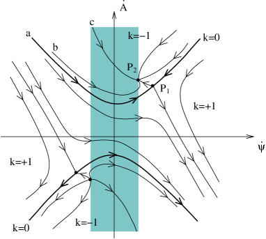
Figure 1: Trajectories in the $\dot{\psi}\dot{A}$–plane for $1<a<\sqrt{4/3}$. When $\sqrt{4/3}<a<\sqrt{3}$ the diagram is similar but the trajectories spiral around the stable attractors. These are the two regimes associated with hyperbolic compactifications. Inside the shaded region the universe is accelerating, whereas outside it decelerates.

Let us analyse the various trajectories in the $\dot{\psi}\dot{A}$–plane drawn in [18], and check whether they correspond to an accelerating universe. Consider first the case of a closed universe. Then, for $a<1$ there are trajectories in the phase plane which exhibit late–time acceleration. These trajectories flow towards the attractor $P_{1}$ which is located inside the acceleration stripe. As shown in [18], the scale factor has the power law behaviour $S\propto\tau^{1/a^{2}}$ and therefore the geometry has a future event horizon. On the other hand, for $a\geq 1$, which includes M–theory compactifications, there is a runaway behaviour with a decelerating universe, as can be seen in both figures 1 and 2.

Next, let us consider the fixed point $P_{1}$, by concentrating, for the moment, on a flat universe with $k=0$. The class of solutions for a flat universe and arbitrary constant $a$ were found explicitly in [16]. For $0<a<\sqrt{3}$, the point $P_{1}$ is always an attractor, if we restrict to the $k=0$ hyperbola. For $a<1$, and therefore not for hyperbolic nor flux compactifications, the fixed point has $\dot{\psi}^{2}<1$. Hence, the asymptotic solution is accelerating. The case $a=1$ has a solution which accelerates and a solution which decelerates, depending if one starts from $\dot{\psi}=\mp\infty$. In particular, the accelerating solution does not have a future event horizon [16]. Within the range $1<a<\sqrt{3}$, which includes hyperbolic compactifications, the asymptotic solution is always decelerating (figure 1). For example, following [4], consider the trajectory (a) in figure 1, starting with large negative $\dot{\psi}$ (the field rolling up the potential). Then, as $\dot{\psi}^{2}$ becomes less then $1$, we enter into a period of transient acceleration, followed again by a period of deceleration. Finally, for $a>\sqrt{3}$, the $k=0$ trajectory (a) of figure 2, associated to flux compactifications, has a runaway behaviour, going through a period of transient acceleration.

\begin{picture}(0.0,0.0)(0.0,0.0)\end{picture}

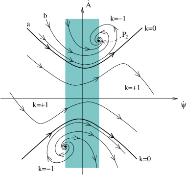
Figure 2: Trajectories in the $\dot{\psi}\dot{A}$–plane for $a>\sqrt{3}$, corresponding to flux compactifications. For open cosmologies, the late time behaviour of the acceleration is always oscillatory.

Let us move to the case of $k=-1$, with $a>1$, where there is always an attractor at $P_{2}$. Note that $P_{2}$ is on the boundary of the region $\dot{\psi}^{2}<1$ of acceleration, because at late times curvature dominates and one has linear expansion. Consequently, these geometries do not have a future event horizon. The behaviour of the trajectories converging to $P_{1}$ changes at $a=\sqrt{4/3}$ (see [18] for details). For $a<\sqrt{4/3}$ the trajectories are as in figure 1, whereas for $a>\sqrt{4/3}$ the trajectories spiral to $P_{2}$, like in figure 2. Whenever $a<\sqrt{4/3}$, we can arrange initial conditions to have a period of transient acceleration similar to the $k=0$ case, as in the trajectory (b) in figure 1. Other initial conditions will give a cosmology with a late time decaying acceleration, as for the trajectory (c) in the same figure. When $a>\sqrt{4/3}$ (so, in particular, for all flux compactifications and for hyperbolic compactifications with $n<6$), independently of initial conditions, we have a cyclic behaviour, with the acceleration oscillating around zero, with decreasing magnitude.

It is now clear that, for flat universes, a positive acceleration is always transient for both type of compactifications and one always has late–time deceleration. This is in contrast with open cosmologies, where both compactifications can give, at late times, periods of positive acceleration. In the following we shall study the behaviour of this late–time acceleration as a function of proper time.

Let us then analyse the dynamical system near the attractor $P_{2}$. After the standard linearization, one obtains the asymptotic behaviour

$$\left(\begin{array}[]{c}\dot{\psi}\\ \dot{A}\end{array}\right)=\left(\begin{array}[]{c}1\\ a/2\end{array}\right)+\left(\begin{array}[]{c}V_{1}\\ V_{2}\end{array}\right)\,e^{\lambda_{+}t}+\left(\begin{array}[]{c}W_{1}\\ W_{2}\end{array}\right)\,e^{\lambda_{-}t}\ ,$$ (3)

where ${\bf V}$ and ${\bf W}$ are the eigenvectors, and the eigenvalues are

$$\lambda_{\pm}=\frac{1}{2}\,\left(-a\pm\sqrt{\Delta}\right)\ ,\ \ \ \ \ \ \ \ \ \ \ \ \ \Delta=4-3a^{2}\ .$$

It is then straightforward to determine the proper time as a function of the time coordinate $t$ which, to leading order, is

$$\tau=\tau_{0}\,\exp\left(\,{\frac{a}{2}\,t}\,\right)+\cdots\ .$$ (4)

Integrating equation (3) and replacing in the general formula for the acceleration (2), one obtains the following asymptotic behaviour as a function of proper time

$$\frac{d^{2}S}{d\tau^{2}}=\frac{1}{\tau^{2}}\,\left(\alpha_{+}\,\tau^{\,\frac{\sqrt{\Delta}}{a}}+\alpha_{-}\,\tau^{\,-\frac{\sqrt{\Delta}}{a}}\right)\ ,$$ (5)

where $\alpha_{\pm}$ are integration constants.

Consider first $a\leq\sqrt{4/3}$, corresponding to real eigenvalues. Then the asymptotic behaviour for the acceleration reads

$$\frac{d^{2}S}{d\tau^{2}}\propto\tau^{-2+\frac{\sqrt{\Delta}}{a}}\ .$$

On the other hand, for $a>\sqrt{4/3}$ the eigenvalues are complex, thus giving rise to the oscillatory behaviour

$$\frac{d^{2}S}{d\tau^{2}}\propto\tau^{-2}\,\cos\left(\frac{\sqrt{-\Delta}}{a}\,\ln\tau+\varphi\right)\ ,$$

where $\varphi$ is a phase. Hence the acceleration will oscillate with an amplitude decreasing as $\tau^{-2}$, falling faster then in the case with $a\leq\sqrt{4/3}$. The periods of acceleration and deceleration become longer as $\tau\rightarrow\infty$. In fact, if the acceleration vanishes at $\tau=\tau_{1}$, then the next zero will occur after an interval

$$\delta\tau=\tau_{1}\left(e^{\beta}-1\right)\ ,\ \ \ \ \ \ \ \ \ \ \ \ \ \ \beta=\frac{\pi a}{\sqrt{-\Delta}}\ .$$

Thus periods of acceleration or deceleration grow linearly with cosmological time.

Finally, it is tempting to define an effective matter and an effective cosmological constant associated with the scalar field by writing the deceleration and total density parameters as

$$q=-\frac{S^{\prime\prime}S}{S^{\prime}{}^{2}}=\frac{\Omega_{M}}{2}-\Omega_{\Lambda}\,,$$

$$\Omega=1+\frac{k}{S^{\prime}{}^{2}}=\Omega_{M}+\Omega_{\Lambda}\,,$$

where primes denote derivatives with respect to proper time $\tau$. Inverting this system of equations we conclude that lines of constant $\Omega_{M}$ are straight lines and lines of constant $\Omega_{\Lambda}$ are ellipses, respectively given by

$$6\,\Omega_{M}\dot{A}^{2}=\dot{\psi}^{2}\ ,\ \ \ \ \ \ \ \ \ 6\,\Omega_{\Lambda}\dot{A}^{2}+\frac{\dot{\psi}^{2}}{2}=1\ .$$

At the attractor, $P_{2}$, one has $\Omega_{M}=2\Omega_{\Lambda}=2/3a^{2}$ while at the saddle point, $P_{1}$, one has $\Omega_{M}=1-\Omega_{\Lambda}=2a^{2}/3$. The present acceleration of the universe derived from supernovae measurements of the $q$ parameter, can then be generically reproduced by trajectories on their way to the attractor. For example, trajectories like (b) in both figures go through an accelerating phase compatible with supernovae observations. Also, it is clear that the system evolves towards an attractor where $\Omega_{M}\sim\Omega_{\Lambda}$, therefore it would not be surprising that both components were of the same order today. This fact could explain the cosmic coincidence problem if the late time dynamics of the universe is determined by the compactification scalar. Notice that, usually one thinks of the quintessence field as the source of dark energy only. Here one is naively assuming that both dark matter and dark energy are generated by the quintessence field alone. While this interpretation seems to resolve the coincidence problem it raises serious problems for small scale structure formation. In fact, even if it is possible to have acceptable growth of baryonic perturbations, it turns out that the perturbations on the Newtonian potential caused by the coupling of the scalar field to gravity do not grow, and therefore cannot explain the mysterious dark matter. Alternatively, we could study the evolution of this model coupled to additional matter. In particular, it would be interesting to investigate if it evolves to a period of eternal acceleration with $\Omega_{M}\sim\Omega_{\Lambda}$.

References

- [1] G. W. Gibbons, Aspects of supergravity theories in Supergravity and related topics, eds. F. de Aguila, J. A. de Azcaárraga and L. Ibañez, (World Scientific, 1985).
- [2] J. M. Maldacena and C. Nunez, Supergravity description of field theories on curved manifolds and a no go theorem, Int. J. Mod. Phys. A 16 (2001) 822, hep-th/0007018.
- [3] L. Cornalba and M. S. Costa, A new cosmological scenario in string theory, Phys. Rev. D 66 (2002) 066001, hep-th/0203031.
- [4] P. K. Townsend and M. N. Wohlfarth, Accelerating cosmologies from compactification, Phys. Rev. Lett. 91 (2003) 061302, hep-th/0303097.
- [5] N. Ohta, Accelerating cosmologies from S–branes, Phys. Rev. Lett. 91 (2003) 061303, hep-th/0303238.
- [6] S. Roy, Accelerating cosmologies from M/string theory compactifications, Phys. Lett. B 567 (2003) 322, hep-th/0304084.
- [7] M. N. Wohlfarth, Accelerating cosmologies and a phase transition in M–theory, Phys. Lett. B 563 (2003) 1, hep-th/0304089; Inflationary cosmologies from compactification, hep-th/0307179.
- [8] R. Emparan and J. Garriga, A note on accelerating cosmologies from compactifications and S–branes, JHEP 0305 (2003) 028, hep-th/0304124.
- [9] N. Ohta, A study of accelerating cosmologies from superstring / M theories, Prog. Theor. Phys. 110 (2003) 269, hep-th/0304172.
- [10] C. M. Chen, P. M. Ho, I. P. Neupane and J. E. Wang, A note on acceleration from product space compactification, JHEP 0307 (2003) 017, hep-th/0304177.
- [11] M. Gutperle, R. Kallosh and A. Linde, M/string theory, S-branes and accelerating universe, JCAP 0307 (2003) 001, hep-th/0304225.
- [12] C. P. Burgess, C. Nunez, F. Quevedo, G. Tasinato and I. Zavala, General brane geometries from scalar potentials: Gauged supergravities and accelerating universes, JHEP 0308 (2003) 056, hep-th/0305211.
- [13] C. M. Chen, P. M. Ho, I. P. Neupane, N. Ohta and J. E. Wang, Hyperbolic space cosmologies, hep-th/0306291.
- [14] S. Nojiri and S. D. Odintsov, Where new gravitational physics comes from: M–theory, hep-th/0307071.
- [15] V. D. Ivashchuk, V. N. Melnikov and A. B. Selivanov, Cosmological solutions in multidimensional model with multiple exponential potential, JHEP 0309 (2003) 059, hep-th/0308113.
- [16] P. K. Townsend, Cosmic acceleration and M–theory, hep-th/0308149.
- [17] I. P. Neupane, Inflation from string/M–theory compactification?, hep-th/0309139; Accelerating cosmologies from exponential potentials, hep-th/0311071.
- [18] J. J. Halliwell, Scalar Fields In Cosmology With An Exponential Potential, Phys. Lett. B 185 (1987) 341.