Distributions of Dirac Operator Eigenvalues

Abstract

The distribution of individual Dirac eigenvalues is derived by relating them to the density and higher eigenvalue correlation functions. The relations are general and hold for any gauge theory coupled to fermions under certain conditions which are stated. As a special case, we give examples of the lowest-lying eigenvalue distributions for QCD-like gauge theories without making use of earlier results based on the relation to Random Matrix Theory.

SPhT-T03/177

1 Introduction

Consider the partition function of Yang-Mills theory coupled vector-like to fermionic matter in a given representation of the gauge group. Integrating out the $N_{f}$ fermions in the Euclidean partition function one obtains the formal expression

$${\cal Z}~{}=~{}\int\![dA]~{}\prod_{f=1}^{N_{f}}\det[i\,\raisebox{0.6458pt}{/}D(A)-m_{f}]\ \exp\left[-S[A]\right]~{},$$ (1.1)

where $S[A]$ is the pure gauge theory action. This involves the determinant of the Dirac operator $\,\raisebox{0.6458pt}{/}D$ (plus the mass terms). One way to make the evaluation of this determinant meaningful is to regularize the theory in such a way that there is a finite number of Dirac operator eigenvalues $\lambda_{i}$.

A regularization of the theory in such a way already exists: lattice gauge theory with a finite lattice spacing $a$ and a finite four-volume $V$. Because of chiral symmetry and the index theorem the spectrum of the Dirac operator eigenvalues is constrained: the spectral density $\rho(\lambda)$ will be symmetric around the origin, $\rho(\lambda)=\rho(-\lambda)$, and there will, for any given gauge field configuration, be a number $\nu$ of exact zero modes. This number of zero modes is dictated by the index theorem.

What will be the distribution of the remaining eigenvalues? The spectral density gives the overall distribution of the unordered set of eigenvalues, but one would like to ask more detailed questions. Here the lattice gauge theory approach offers a fruitful angle to the problem. It is thus instructive to view the path integral over the gauge field $A_{\mu}(x)$ as the limit of a discrete sum over gauge field configurations. For each gauge field configuration one will have a set of non-zero Dirac operator eigenvalues $\lambda_{i}$, where, because of the spectral symmetry, only the $N$ positive ones need to be considered here. These eigenvalues can be ordered according to their magnitudes, $\lambda_{1}<\lambda_{2}<\ldots<\lambda_{N}$. Performing this ordering configuration by configuration, one can ask for the individual distribution of the $k$th Dirac operator eigenvalue. It is far from obvious how one would go about computing such individual distributions of ordered Dirac operator eigenvalues directly from first principles and the quantized gauge field theory. In fact, it is surprising how little apparently can be said from first principles. The only rigorous statement we have been able to find in the literature is the inequality [1]

$$\lambda_{1}\leq\frac{C}{L}~{},$$ (1.2)

where $\lambda_{1}$ is the smallest non-zero eigenvalue, $C$ is a constant, and $L$ is the linear extent of the four-volume. All this says is that the smallest eigenvalue $\lambda_{1}$ approaches zero in the limit $L\to\infty$ at a rate which is not slower than that of free fields. This should be contrasted with what one obtains if one in addition assumes spontaneous chiral symmetry breaking. From the Banks-Casher relation [2]

$$\rho(0)=L^{4}\Sigma/\pi~{},$$ (1.3)

where $\Sigma$ is the chiral condensate, it follows that a non-vanishing $\Sigma$ requires the Dirac operator eigenvalues to accumulate at substantially faster rate, yielding (with some other constant $\tilde{C}$) [3]

$$\lambda_{1}\leq\frac{\tilde{C}}{L^{4}}~{}.$$ (1.4)

This has been succinctly rephrased by Shuryak and Verbaarschot [4]: Spontaneous chiral symmetry breaking and the required accumulation of eigenvalues near the origin according to (1.4) suggests that a more appropriate object to study near $\lambda\sim 0$ is the so-called microscopic spectral density [4],

$$\rho_{s}(\zeta)~{}\equiv~{}\frac{1}{\Sigma V}\rho\left(\lambda=\frac{\zeta}{\Sigma V}\right)~{}.$$ (1.5)

Remarkably, it has turned out that this microscopic spectral density is computable analytically using the relation to the appropriate low-energy effective field theory, a chiral Lagrangian [5]. What is perhaps more astonishing, the same results can be obtained from universality classes of large-$N$ (chiral) Random Matrix Theories [4, 6, 7, 8]. To be precise, using the relation to effective field theory it has been shown how to derive the microscopic spectral density $\rho_{s}(\zeta)$ [5] and spectral two-point function [9] for the symmetry breaking class of QCD. For the two remaining symmetry breaking classes the corresponding effective field theories have been compared perturbatively to the microscopic spectral density from chiral Random Matrix Theory [10]. For the symmetry breaking class of QCD the procedure for deriving the higher $k$-point spectral correlation functions using effective field theory is completely clear, and it is only computational tedium that has so far prevented the calculation of higher $k$-point functions. Very compact expressions for these spectral $k$-point functions are known if one accepts the conjecture of the relation to Random Matrix Theory, and the relevant generating functional which eventually should be derived from field theory is also known explicitly [11, 12]. But in this paper we will not rely on chiral Random Matrix Theory at all, and therefore we shall not make use of these explicit results, even though they are almost certainly in agreement in what one will obtain from effective field theory.

The purpose of this paper is to point out that even the distribution of individual Dirac operator eigenvalues can be computed directly from effective field theory. This may seem surprising, because the concept of an ordered set of Dirac operator eigenvalues is not obviously related to quantum field theory observables. But following the program described in refs. [5], it is clear how to proceed if one instead wishes to derive all spectral correlation functions. Having all spectral correlation functions there should be no more spectral information in the theory, and individual eigenvalue distributions ought to follow. This is indeed the case. In fact, the derivation will be completely general, and can be phrased in terms of fundamental notions from probability theory and certain assumptions regarding the regularized QCD partition function which we will state explicitly below. In particular, the discussion will not be restricted to the “$\epsilon$-regime” of QCD, although this clearly is an important special case. The counting of eigenvalues from the origin can trivially be replaced by the counting from any other arbitrary point in the spectrum.

2 Spectral Correlation Functions and Eigenvalue Distributions

To proceed, we need precise definitions of the spectral correlation functions. We remind the reader that we consider a situation in which we have a finite number of Dirac operator eigenvalues, and we focus on the $N$ eigenvalues lying above zero. To even define spectral correlation functions of these $N$ Dirac operator eigenvalues $\lambda_{i=1,\ldots,N}$ we must assume the existence of a joint probability distribution function ${\cal P}_{N}(\lambda_{1},\ldots,\lambda_{N})$. For simplicity we will here assume that this function has support on the whole space of ${\mathbf{R}}_{+}^{N}$ (the restriction to a subset hereof is immaterial for the discussion that follows, and is readily implemented). We will also assume that ${\cal P}_{N}(\lambda_{1},\ldots,\lambda_{N})$ is symmetric under interchange of all arguments. We choose the normalization convention

$$\int_{0}^{\infty}\!d\lambda_{1}\ldots d\lambda_{N}~{}{\cal P}_{N}(\lambda_{1},\ldots,\lambda_{N})~{}=~{}1~{}.$$ (2.1)

The limit $N\to\infty$ is easily taken in all formulas that follow below.

The $k$-point density correlation function, which gives the probability density to find the $k$ variables at values $\lambda_{1},\ldots,\lambda_{k}$ is then

$$\rho_{k}(\lambda_{1},\ldots,\lambda_{k})\ \equiv\ \frac{N!}{(N-k)!}\int_{0}^{\infty}d\lambda_{k+1}\ldots d\lambda_{N}\,{\cal P}_{N}(\lambda_{1},\ldots,\lambda_{N})\ .$$ (2.2)

In quantum field theory one is most used to considering just the one-point function, the spectral density $\rho(\lambda)$. As follows, it is obtained by integrating the joint probability density over $N-1$ variables, $viz.$

$$\rho(\lambda)=N\int_{0}^{\infty}\!d\lambda_{2}\ldots d\lambda_{N}{\cal P}_{N}(\lambda,\lambda_{2},\ldots,\lambda_{N})~{},$$ (2.3)

the factor of $N$ easily being understood as due to having arbitrarily chosen to keep just the first entry fixed while integrating out the rest. The existence of a joint probability density ${\cal P}_{N}(\lambda_{1},\ldots,\lambda_{N})$ is implicit in all work that considers the spectral density and higher spectral correlation functions of the Dirac operator in QCD and related field theories. In particular, the $N$-point function is simply proportional to the joint probability distribution function itself, $\rho_{N}(\lambda_{1},\ldots,\lambda_{N})=N!\,{\cal P}_{N}(\lambda_{1},\ldots,\lambda_{N})$.

It is useful to also define a $k$-th “gap probability”. For simplicity, let us restrict ourselves to a gap adjacent to the origin; it is straightforward to pick any other fixed interval on the support of the eigenvalues. Define

$$E_{k}(s)\ \equiv\ \frac{N!}{(N-k)!}\int_{0}^{s}d\lambda_{1}\ldots d\lambda_{k}\int_{s}^{\infty}d\lambda_{k+1}\ldots d\lambda_{N}\,{\cal P}_{N}(\lambda_{1},\ldots,\lambda_{N})\ ,\ \ \mbox{for}\ k=0,1,\ldots,N\ \ .$$ (2.4)

For $k=0$ this gives the probability that all variables are larger or equal to $s$, $\lambda_{i=1,\ldots,N}\geq s$, meaning that the interval $[0,s]$ is free of eigenvalues. For general $k$ the interval $[0,s]$ is occupied by $k$ eigenvalues and $[s,\infty)$ is occupied by $N-k$ eigenvalues. Our first step consists in proving that the $k$-th gap probability can be written as a sum of integrals over $(N-k+1)$ different $l$-point functions. We use the simple identity

$$(a-b)^{j}\ =\ \sum_{l=0}^{j}(-1)^{l}{j\choose l}a^{j-l}b^{l}\ ,$$ (2.5)

and choose $a=\int_{0}^{\infty}d\lambda$ and $b=\int_{0}^{s}d\lambda$ to replace all the $(N-k)$ integrals $\int_{s}^{\infty}d\lambda$ in eq. (2.4) by $a-b$:

$$E_{k}(s) = \frac{N!}{(N-k)!}\int_{0}^{s}d\lambda_{1}\ldots d\lambda_{k}$$ (2.6)

$$\times\sum_{l=0}^{N-k}(-1)^{l}{N-k\choose l}\left(\int_{0}^{\infty}\right)^{N-k-l}\left(\int_{0}^{s}\right)^{l}d\lambda_{k+1}\ldots d\lambda_{N}\,{\cal P}_{N}(\lambda_{1},\ldots,\lambda_{N})$$

$$= \sum_{l=0}^{N-k}(-1)^{l}\frac{1}{l!}\int_{0}^{s}d\lambda_{1}\ldots d\lambda_{k+l}\ \rho_{k+l}(\lambda_{1},\ldots,\lambda_{k+l})\ .$$

Here we have used the invariance of ${\cal P}_{N}(\lambda_{1},\ldots,\lambda_{N})$ under permutations. The formula (2.6) neatly expresses the gap probability in terms of spectral correlation functions [13]. For the simplest case of $k=0$ we get

$$E_{0}(s)\ =\ 1\ -\ \int_{0}^{s}d\lambda_{1}\,\rho_{1}(\lambda_{1})\ +\ \frac{1}{2}\int_{0}^{s}d\lambda_{1}d\lambda_{2}\,\rho_{2}(\lambda_{1},\lambda_{2})\ -\frac{1}{6}\int_{0}^{s}d\lambda_{1}d\lambda_{2}d\lambda_{3}\rho_{3}(\lambda_{1},\lambda_{2},\lambda_{3})+\ \ldots~{}.$$ (2.7)

We may also introduce a generating functional for all gap probabilities, defined as [13]

$$E(s;\xi)\ \equiv\ 1+\sum_{l=1}^{N}(-\xi)^{l}\frac{1}{l!}\int_{0}^{s}d\lambda_{1}\ldots d\lambda_{l}\ \rho_{l}(\lambda_{1},\ldots,\lambda_{l})\ .$$ (2.8)

It immediately follows that

$$E_{k}(s)\ =\ (-1)^{k}\left.\frac{\partial^{k}}{\partial\xi^{k}}\ E(s;\xi)\right|_{\xi=1}\ ,\ \ \mbox{for}\ k=0,1,\ldots,N\ \ .$$ (2.9)

The probability to find the $k$-th eigenvalue at value $\lambda_{k}=s$ is

$$p_{k}(s)\ \equiv\ k{N\choose k}\int_{0}^{s}d\lambda_{1}\ldots d\lambda_{k-1}\int_{s}^{\infty}d\lambda_{k+1}\ldots d\lambda_{N}\,{\cal P}_{N}(\lambda_{1},\ldots,\lambda_{k-1},\lambda_{k}=s,\lambda_{k+1},\ldots,\lambda_{N})\ .$$ (2.10)

If we order the eigenvalues, $\lambda_{1}<\ldots<\lambda_{N}$, the quantity $p_{k}(s)$ gives the probability to find the $k$-th eigenvalue in this ordering at $\lambda_{k}=s$, as eq.(2.10) gives the probability to find $k-1$ eigenvalues in $[0,s]$, $\lambda_{k}=s$, and $N-k$ eigenvalues in the complement $[s,\infty)$. It is shown in Appendix A that the distributions of eigenvalues $p_{k}(s)$ are indeed all properly normalized, $\int_{0}^{\infty}ds\ p_{k}(s)=1$ for all $k=1,\ldots,N$.

If we compare eq. (2.10) and eq. (2.4) for $k-1$ we observe that they differ only by one integration. By differentiating we thus easily obtain

$$\frac{\partial}{\partial s}E_{k}(s)\ =\ k!\,\left(p_{k}(s)-p_{k+1}(s)\right)\ ,$$ (2.11)

defining $p_{0}(s)\equiv 0$. Here we have again made use of the permutation symmetry of the integrand, renaming the variable of the differentiated integrals by $\lambda_{k}$. Inserting eq. (2.6) or eq. (2.9) we can thus recursively determine the distribution of the $k$-th individual eigenvalue from the knowledge of all density correlation functions alone. This confirms the intuition mentioned in the introduction that if all spectral correlations are known, no more spectral information can be gleaned.

Let us give some examples. For the first eigenvalue we obtain

$$p_{1}(s)\ =\ -\frac{\partial}{\partial s}E_{0}(s)\ =\ \rho_{1}(s)-\int_{0}^{s}d\lambda\,\rho_{2}(\lambda,s)\ +\ldots\ ,$$ (2.12)

by a single differentiation of eq. (2.7), whereas the second eigenvalue is given by

$$p_{2}(s)\ =\ \int_{0}^{s}d\lambda\,\rho_{2}(\lambda,s)\ +\ \ldots\ \ .$$ (2.13)

This explicitly confirms the expectation that the first approximation to the smallest of these ordered eigenvalues is given by the spectral density itself. The higher order correlation functions systematically correct for the error in this initial approximation. As we shall show below for the case of the microscopic spectrum of the Dirac operator, the convergence can be remarkably fast. Proceeding recursively, an infinite sequence of eigenvalue distributions follows from eq. (2.11).

3 Distributions of Dirac Operator Eigenvalues in the $\epsilon$-Regime

An obvious place to apply the above general formalism is near the origin. As mentioned in the introduction, if one assumes that chiral symmetry is broken spontaneously the spectral correlation functions for the lowest-lying Dirac operator eigenvalues can be computed analytically. The bridge is an effective field theory which hinges on the precise Goldstone boson manifold, and the pertinent field theory is taken to a corner known as the $\epsilon$-regime [14] by a suitable tuning of the four-volume $V$. Let us mention that if we want to compare the regularized gauge theory with a finite number of eigenvalues $N$ to such an effective theory we must assume that this number $N$ is large.

The density correlation functions and thus also the distributions of eigenvalues depend on the number of flavors $N_{f}$, quark masses $m_{f}$ and gauge field topology $\nu$. There have been several numerical simulations of individual Dirac eigenvalue distributions both using staggered fermions (see, $e.g.$, refs. [15, 16]) and overlap fermions [17, 18, 19]. So far it is has only been possible to compare with the analytical predictions based on the conjectured Random Matrix Theory results [20, 21], and an outstanding question has been whether these individual eigenvalue distributions also can be derived directly from the effective field theory. We will here rely only on what to date has been derived from field theory, namely the one- and two-point functions for the symmetry breaking class of QCD-like gauge theories (gauge theories with fermions transforming according to complex representations of the gauge group) [5, 9].

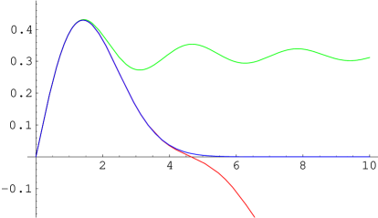
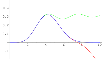
Figure 1: The distribution of the first Dirac eigenvalue for $N_{f}=0$ and $|\nu|=0,1,2$. The first term (green) and the sum of first and second term (red) in the expansion eq. (2.12) are compared to the full result from Random Matrix Theory (blue) summing over all density correlations.

For simplicity of illustration we restrict ourselves to massless quarks. The microscopic spectral density eq. (1.5) for $N_{f}$ massless flavors in a sector of topological charge $\nu$ derived in [5] reads

$$\rho_{s}^{(N_{f},\,\nu)}(\zeta)\ =\ \frac{\zeta}{2}\left[J^{2}_{N_{f}+|\nu|}(\zeta)-J_{N_{f}+|\nu|+1}(\zeta)J_{N_{f}+|\nu|-1}(\zeta)\right]\ ,$$ (3.1)

in terms of the rescaled eigenvalues $\zeta=\lambda V\Sigma$. The two-point function has been derived so far only for zero flavors $N_{f}=0$ and arbitrary $\nu\neq 0$

$$\rho_{s}^{(N_{f}=0,\,\nu)}(\zeta,\eta)\ =\ \rho_{s}^{(0,\,\nu)}(\zeta)\rho_{s}^{(0,\,\nu)}(\eta)-\frac{\zeta\eta}{(\zeta^{2}-\eta^{2})^{2}}\left[\zeta J_{|\nu|+1}(\zeta)J_{|\nu|}(\eta)-\eta J_{|\nu|+1}(\eta)J_{|\nu|}(\zeta)\right]^{2}~{}.$$ (3.2)

We can now give the approximate distribution of the first Dirac Eigenvalue as it follows from the effective field theory to this order by inserting the above equations into eq. (2.12). This is shown in Fig. 1 for three different values of $\nu$. Clearly the approximation cannot be trusted in the region where, to this order, $p_{1}^{(\nu)}(\zeta)$ goes negative. However, the comparison to the full result as it is conjectured from Random Matrix Theory [20] shows that for all practical purposes even this approximation that keeps only the two leading terms in the expansion is sufficient when comparing with lattice data.

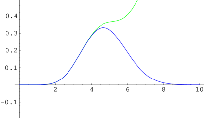
Figure 2: The distribution of the second Dirac eigenvalue for $\nu=0$. The leading order term from eq. (2.13) (green) is plotted versus the full result (blue).

From eq. (2.13) and the knowledge of the two-point function eq. (3.2) we can also give the leading term in the expansion for the second Dirac eigenvalue, see Fig. 2. This 2nd eigenvalue distribution is described very accurately almost up to its maximum if we compare to Random Matrix Theory [21]. To get the same degree of accuracy as for the first eigenvalue we would need the three-point function, which has not yet been derived from the chiral Lagrangian. But we hope these examples suffice to illustrate how individual lowest-lying eigenvalue distributions of the Dirac operator can be obtained from the effective Lagrangian framework.

4 Conclusions

We have shown that the distribution of individual Dirac operator eigenvalues can be computed solely from the knowledge of eigenvalue density correlations function. Since a well-established procedure exists for deriving all $k$-point spectral correlation functions from field theory, this settles the question as to how one can also derive from field theory individual eigenvalue distributions of the Dirac operator. We have illustrated the method with a case where exact analytical results already have been derived from field theory, namely the lowest-lying Dirac eigenvalues in QCD-like theories which undergo spontaneous chiral symmetry breaking. While it is expected that all eigenvalue correlations in this regime are identical to those obtained from Random Matrix Theory we have not made use of this assumption. We have shown that even just on the basis of the knowledge, to date, of the microscopic one- and two-point density from effective field theory the distribution of the first eigenvalue is indistinguishable from the conjectured analytical result from Random Matrix Theory. The expansion can be pushed to any needed degree of accuracy by computing the required higher $k$-point correlation functions from field theory. This is certainly the case for a physical number of fermions $N_{f}$. The only exception may be the quenched limit of $N_{f}=0$. If this case is inherently ill-defined at the level of the expansion in the effective Lagrangian, not even spectral correlation functions can be reliably computed by the route through effective field theory. An entirely different approach could then be called for. But our relations between individual eigenvalue distributions and spectral correlation functions will remain valid.

Acknowledgments: We wish to thank the CERN Theory Division, where part of this work was being done, for hospitality. The work of GA was supported by a Heisenberg fellowship of the Deutsche Forschungsgemeinschaft.

Appendix A Appendix A

Here we show that the distribution of the $k$-th eigenvalue eq. (2.10) is normalized to unity for all $k$:

$$\int_{0}^{\infty}ds\,p_{k}(s)\ =$$

$$= k{N\choose k}\int_{0}^{\infty}ds\int_{0}^{s}d\lambda_{1}\ldots d\lambda_{k-1}\int_{s}^{\infty}d\lambda_{k+1}\ldots d\lambda_{N}\,{\cal P}_{N}(\lambda_{1},\ldots,\lambda_{k-1},s,\lambda_{k+1},\ldots,\lambda_{N})$$

$$= k{N\choose k}\sum_{l=0}^{k-1}(-1)^{l}{k-1\choose l}\int_{0}^{\infty}ds\left(\int_{0}^{\infty}\right)^{k-l-1}\left(\int_{s}^{\infty}\right)^{N-k+l}\!\!d\lambda_{1}\ldots d\lambda_{k-1}d\lambda_{k+1}\ldots d\lambda_{N}$$

$$\ \ \ \ \ \ \ \ \ \ \ \ \ \ \ \ \ \ \ \ \ \ \ \ \ \ \ \ \ \ \ \ \ \ \ \ \ \ \ \ \ \ \ \ \ \ \ \ \ \ \ \ \ \ \ \ \ \ \ \ \ \times\ \,{\cal P}_{N}(\lambda_{1},\ldots,\lambda_{k-1},s,\lambda_{k+1},\ldots,\lambda_{N})\ .$$

We have used again the identity eq. (2.5) choosing $a=\int_{0}^{\infty}d\lambda$ and $b=\int_{s}^{\infty}d\lambda$ in order to replace the integrals $\int_{0}^{s}d\lambda$. We next order the integration variables of the $(N-k+l)$ integrations over $[s,\infty)$,

$$\int_{0}^{\infty}ds\left(\int_{s}^{\infty}\right)^{N-k+l}d\lambda_{k-l+1}\ldots d\lambda_{N}\,{\cal P}_{N}(\lambda_{1},\ldots,\lambda_{k-1},s,\lambda_{k+1},\ldots,\lambda_{N})\ =$$

$$= (N-k+l)!\int_{0}^{\infty}ds\int_{s}^{\infty}d\lambda_{k-l+1}\int_{\lambda_{k-l+1}}^{\infty}d\lambda_{k-l+2}\ldots\int_{\lambda_{N-1}}^{\infty}d\lambda_{N}$$

$$\ \ \ \ \ \ \ \ \ \ \ \ \ \ \ \ \ \ \ \ \ \ \ \ \ \ \ \ \ \ \ \ \ \ \ \ \ \ \ \ \ \ \ \ \ \ \ \ \ \ \ \ \ \ \ \ \ \ \ \ \ \times\ \,{\cal P}_{N}(\lambda_{1},\ldots,\lambda_{k-1},s,\lambda_{k+1},\ldots,\lambda_{N})$$

$$= \frac{1}{N-k+l+1}\left(\int_{0}^{\infty}\right)^{N-k+l+1}ds\,d\lambda_{k-l+1}\ldots d\lambda_{N}\,{\cal P}_{N}(\lambda_{1},\ldots,\lambda_{k-1},s,\lambda_{k+1},\ldots,\lambda_{N})\ ,$$

and then undo the ordering with the additional integration over $s$. Inserting eq. (A) into eq. (A) all the integrations over the joint probability distribution will give unity and we arrive at

$$\int_{0}^{\infty}ds\ p_{k}(s)\ =\ k{N\choose k}\sum_{l=0}^{k-1}(-1)^{l}{k-1\choose l}\frac{1}{N-k+l+1}\ =\ 1.$$ (A.3)

References

- [1] C. Vafa and E. Witten, Commun. Math. Phys. 95 (1984) 257.
- [2] T. Banks and A. Casher, Nucl. Phys. B 169 (1980) 103.
- [3] H. Leutwyler and A. Smilga, Phys. Rev. D 46 (1992) 5607.
- [4] E. V. Shuryak and J. J. Verbaarschot, Nucl. Phys. A 560 (1993) 306 [hep-th/9212088].
- [5] J. C. Osborn, D. Toublan and J. J. Verbaarschot, Nucl. Phys. B 540 (1999) 317 [hep-th/9806110]; P. H. Damgaard, J. C. Osborn, D. Toublan and J. J. Verbaarschot, Nucl. Phys. B 547 (1999) 305 [hep-th/9811212].
- [6] J. J. Verbaarschot and I. Zahed, Phys. Rev. Lett. 70 (1993) 3852 [hep-th/9303012].
- [7] J. J. Verbaarschot, Nucl. Phys. B 426 (1994) 559 [hep-th/9401092].
- [8] G. Akemann, P. H. Damgaard, U. Magnea and S. Nishigaki, Nucl. Phys. B 487 (1997) 721 [hep-th/9609174].
- [9] D. Toublan and J. J. M. Verbaarschot, Nucl. Phys. B 603 (2001) 343 [hep-th/0012144]; K. Splittorff and J. J. M. Verbaarschot, hep-th/0310271.
- [10] D. Toublan and J. J. Verbaarschot, Nucl. Phys. B 560 (1999) 259 [hep-th/9904199].
- [11] K. Splittorff and J. J. M. Verbaarschot, Phys. Rev. Lett. 90 (2003) 041601 [cond-mat/0209594].
- [12] Y. V. Fyodorov and G. Akemann, JETP Lett. 77 (2003) 438 [Pisma Zh. Eksp. Teor. Fiz. 77 (2003) 513] [cond-mat/0210647].
- [13] A. Borodin and P. J. Forrester, math-ph/0205007; P. J. Forrester and E. M. Rains, math-ph/0211041.
- [14] J. Gasser and H. Leutwyler, Phys. Lett. B 188 (1987) 477.
- [15] M. E. Berbenni-Bitsch, S. Meyer, A. Schafer, J. J. M. Verbaarschot and T. Wettig, Phys. Rev. Lett. 80 (1998) 1146 [hep-lat/9704018].
- [16] P. H. Damgaard, U. M. Heller, R. Niclasen and K. Rummukainen, Phys. Lett. B 495 (2000) 263 [hep-lat/0007041].
- [17] R. G. Edwards, U. M. Heller, J. E. Kiskis and R. Narayanan, Phys. Rev. Lett. 82 (1999) 4188 [hep-th/9902117].
- [18] W. Bietenholz, K. Jansen and S. Shcheredin, JHEP 0307 (2003) 033 [hep-lat/0306022].
- [19] L. Giusti, M. Lüscher, P. Weisz and H. Wittig, hep-lat/0309189.
- [20] S. M. Nishigaki, P. H. Damgaard and T. Wettig, Phys. Rev. D 58 (1998) 087704 [hep-th/9803007].
- [21] P. H. Damgaard and S. M. Nishigaki, Phys. Rev. D 63 (2001) 045012 [hep-th/0006111].