Confinement from new global defect structures

Abstract

We investigate confinement from new global defect structures in three spatial dimensions. The global defects arise in models described by a single real scalar field, governed by special scalar potentials. They appear as electrically, magnetically or dyonically charged structures. We show that they induce confinement, when they are solutions of effective QCD-like field theories in which the vacua are regarded as color dielectric media with an anti-screening property. As expected, in three spatial dimensions the monopole-like global defects generate the Coulomb potential as part of several confining potentials.

I Introduction

We can describe the physics of heavy quarks by using models that engender non relativistic confining potentials. One can successfully obtain the whole mass spectrum of the quark anti-quark pair in the quarkonium system using, for instance, the well-known Cornell potential cornell $U_{C}(r)\!=\!-\frac{a}{r}+br$, where $a,\,b$ are nonnegative constants and $r$ is the distance between quarks. Although there are many different forms of such confining potentials the most probable potential to describe heavy quarks in the bottomonia region, as has been shown in MZ ; Z , is $U_{MZ}(r)\!=\!C_{1}(\sqrt{r}-\frac{C_{2}}{r})$, where the constants are fixed as $C_{1}\simeq 0.71\,{\rm GeV}^{1/2}$ and $C_{2}\simeq 0.46\,{\rm GeV}^{3/2}$ — see slusa for further details.

As one knows the color vacuum in QCD has an analog in QED. In QED the screening effect creates an effective electric charge that increases when the distance $r$ between a pair of electron-antielectron decreases. On the other hand, in QCD there exists an anti-screening effect that creates an effective color charge which decreases when the distance $r$ between a pair of quark-antiquark decreases. We can summarize this discussion by writing $E(r)\sim\frac{q^{\prime}(r)}{r^{2}}\sim\frac{q}{G(r)r^{2}}$, where $E(r)$ stands for the electric (or color electric) field due to a charge $q$ embedded in a polarizable medium characterized by a “(color) dielectric function” $G(r)$ and $r$ represents an arbitrary position on the (color) dielectric medium. The QED vacuum behavior manifests according to the effective electric charge $q^{\prime}(r\gg d)\leq 1$ or $G(r\gg d)\geq 1$ and $q^{\prime}(r\ll d)>1$ or $G(r\ll d)<1$, where $d$ is the typical size of the polarized “molecules”. On the other hand, the QCD vacuum behavior manifests according to the effective $color$ electric charge $q^{\prime}(r\gg R)\gg 1$ or $G(r\gg R)\ll 1$ and $q^{\prime}(r<R)\to 1$ or $G(r<R)\to 1$, where $R$ is the typical radius of a particular hadron made of quarks. Since we are interested on confinement we shall focus our attention on the latter case, where the behavior of $G(r)$ is clearly chosen such that the QCD vacuum provides absolute color confinement. Note that formally we can continue using Abelian gauge fields just as in QED, but now $G(r)$ is chosen properly in order to provide confinement. In fact, as we shall see below, even though we consider non-Abelian gauge fields there are some reasons to consider only the Abelian projections when these fields are embedded in color dielectric medium willets . We account to these facts to study confinement of quarks and gluons inside hadrons by using an effective phenomenological QCD-like field theory mit ; slac ; cornell ; fl .

As an example consider $G(r)\!=\!\frac{a}{a+br^{2}}$. Notice that $G(r\!\to\!\infty)\!\to\!0$ and $G(r\!\to\!0)\!\to\!1$ as expected to provide perfect confinement. Using this function $G(r)$ and the fact that $E(r)\!\sim\!\frac{q}{G(r)r^{2}}$, it is not difficult to conclude that the potential $U(r)$ has the form of the Cornell potential. As we have stated above, there are many different forms of confining potential and then many different color dielectric functions $G(r)$ can be used to describe confinement. However, for simplicity we choose $G(r)$ as simpler as possible. By considering specific color dielectric functions, we shall investigate later models developing several possibilities of confining potentials.

In general, the behavior of the color dielectric function $G$ with respect to $r$ can be driven by some scalar field $\phi(r)$ that describe the dynamics of the color dielectric medium. Applying the Lagrangian formalism to describe both dynamics of gauge and scalar fields embedded in a color dielectric medium we have the effective lagrangian ${\cal L}_{eff}\!=\!-\frac{1}{4}\,G(\phi)F_{\mu\nu}F^{\mu\nu}+\frac{1}{2}\partial_{\mu}\phi\partial^{\mu}\phi-j_{\mu}A^{\mu}$, where $\mu,\nu\!=\!0,1,2,...,D$ and $j_{\mu}$ is an external color current density. Considering static gauge fields, i.e., $A_{\mu}\!=\![U(r),0,...,0]$, $E(r)\!=\!F_{0r}$, $D\!=\!3$ and $j_{0}\!=\!\rho(r)\!=\!4\pi q\delta(r)$, the equation of motion for the gauge field gives $E\!=\!\frac{q}{G(\phi)r^{2}}$ where the function $G(\phi)$ defines the confinement. The color electric charge can be given by the fermionic sector as $j_{\mu}=q\bar{\psi}\gamma_{\mu}\psi$ of a QCD-like theory that we consider in the next section with further detail. Let us now make some comment about the scalar field sector and also consider other assumptions. Theories involving gauge and scalar fields like the effective lagrangian ${\cal L}_{eff}$ above have been well explored in the literature slusa ; dick1 ; dick2 ; dick3 . Specially in dick1 a model involving Abelian projections of non-Abelian gauge field coupled to a dynamical scalar field as in the effective Lagrangian above was considered. The scalar field $\phi$ was identified with dilaton field whose solution of equation of motion behaves like $\phi(r)\sim\ln{(1+\frac{a}{r})}$. The scalar potential $V(\phi)$ is set to zero. It was shown in this model that the Coulomb potential is regularized at short distance. Other investigations as given in slusa ; dick2 ; dick3 usually consider a non-zero scalar potential like $V(\phi)\sim\alpha\phi^{\,\beta}$ which has a unique minimum. We consider below a different perspective of investigation.

Let us consider the possibility of formation of defects in the color dielectric medium. In order to implement this phenomenon the potential $V(\phi)$ should have a set of minima whose topology is nontrivial. These defects can be understood as nonlinear excitations of the color dielectric medium. Since they become charged via fermion zero modes — see details in Sec. II — they carry “color” charges localized along their spatial extensions. We investigate the confinement of these defects since they are charged objects embedded in a color dielectric medium.

In Classical Electrodynamics, as one knows, there are extended charged objects that play the role of confinement. As an example, consider the infinite plane of charges that produces the “confining potential” $U(r)\sim\sigma r$. Notice that this object interacts with charged particles — or with another parallel infinite plane — in such a way that we cannot separate them from each other since the energy of the system increases with the separation $r$. However, other objects with finite size as a charged sphere or radius $R$ produces an electrical field (for $r\!>\!R$) just as the the electrical field of a point particle, i.e., $E\sim\frac{Q}{r^{2}}$, where $Q$ is the total charge of the sphere. Of course, in this case there is no confining behavior since the energy decreases with the separation $r\!>\!R$. On the other hand, as we have stressed above, when such charges are embedded in a dielectric medium with anti-screening property, i.e., in the QCD vacuum, the confinement appears.

Consider a system with gauge fields embedded in medium that develops both dielectric and magnetic property given by the Lagrangian ${\cal L}\!=\!-\frac{1}{4}G(\phi)F_{\mu\nu}F^{\mu\nu}+j_{\mu}A^{\mu}-\frac{1}{4}H(\phi)\widetilde{F}_{\mu\nu}\widetilde{F}^{\mu\nu}+j_{m\mu}\widetilde{A}^{\mu}+\frac{1}{2}\partial_{\mu}\phi\partial^{\mu}\phi$, where $j_{\mu}$ and $j_{m\mu}$ are current densities of electric and magnetic charges either associated to point-like sources or extended charged defects. Assuming that the dual gauge field with strength tensor $\widetilde{F}_{\mu\nu}$ describes magnetic monopoles on the QCD vacuum, we expect that “magnetic permeability” $H(\phi)$ gets stronger as the dielectric function $G(\phi)$ gets weaker and vice-versa — recall that magnetic and electric charges, $h$ and $q$, are related as $h\sim 1/q$. Let us now implement the idea proposed by ’t Hooft and Mandelstam tman — see also Seiberg-Witten theory sbwit — concerning confinement of quarks. It considers magnetic monopoles in the QCD vacuum generating screening currents that confine the color electric flux in a narrow tube. This is dual to the Abrikosov flux tube produced in a superconductor — see, e.g., singh for further discussions. In order to produce confinement, both $G(\phi)$ and $H(\phi)$ should have the suitable behavior $G(r\gg R)\to 0$ ($H(r\gg R)\to 1)$, for the confined phase; and $G(r\lesssim R)\to 1$ ($H(r\lesssim R)\to 0)$, for deconfined phase. $R$ is the radius of the hadron in deconfined phase and $\phi$ is uniform in both regime, i.e., $\partial_{r}\phi(r)\sim 0$. In the confined phase a hadron (such as a quark-anti-quark pair or a defect-anti-defect pair) looks like a narrow flux tube (connecting the two sources) embedded in a monopole condensate. This phenomenon is governed by the dual effective Lagrangian $\widetilde{\cal L}_{eff}\!=\!-\frac{1}{4}\widetilde{F}_{\mu\nu}\widetilde{F}^{\mu\nu}+j_{m\mu}\widetilde{A}^{\mu}$, whose equations of motion are (i) $\nabla{.}\vec{\widetilde{B}}\!=\!\rho_{m}$ and (ii) $-\nabla\times\vec{\widetilde{E}}\!=\!\vec{j}_{m}$, where $\vec{\widetilde{E}}$ and $\vec{\widetilde{B}}$ are static fields and $j_{\mu}\!=\!0$. The homogeneous equation $\nabla{.}\vec{\widetilde{E}}\!=\!0$ describes the uniform electric field in the confined phase. The persistent currents in the monopole condensate are governed by the dual London equation $\lambda^{2}\nabla\times\vec{j_{m}}\!=\!\vec{\widetilde{E}}$, where $\lambda$ is the London penetration depth singh . Combining this equation with Eq.(ii) for the electric field $\vec{\widetilde{E}}$ we find the fluxoid quantization relation $\int{\vec{\widetilde{E}}.d\vec{S}}-\lambda^{2}\oint{\vec{j}_{m}.d\vec{{\ell}}}\!=\!n\Phi_{e}$ singh , where $n$ is an integer and $\Phi_{e}\!=\!q$ is the quantum of electric flux.

On the other hand, in deconfined phase the magnetic monopoles are dilute and the magnetic current is negligible, i.e., $j_{m\mu}\!\sim\!0$. In this regime the theory is described by the effective Lagrangian ${\cal L}_{eff}\!=\!-\frac{1}{4}{F}_{\mu\nu}{F}^{\mu\nu}+j_{\mu}A^{\mu}$, whose equations of motion are (iii) $\nabla{.}\vec{E}\!=\!\rho$ and (iv) $\nabla\times\vec{B}\!=\!\vec{j}$, where $\vec{E}$ and $\vec{B}$ are static fields and the electric current $\vec{j}$ vanishes. The equation (iii) should describe the Coulomb potential in the deconfined phase. The above equations of motion comprise part of the full set of equations of motion we obtain from the original Lagrangian for the scalar, electric and magnetic fields — fermion fields will also be included later. In deconfined phase, since there are some magnetic monopoles, they are around the surface of the hadron. The magnetic field due to such magnetic monopoles can be found by using the “Gauss law” (i) in $D$-spatial dimensions given as (v) $\frac{1}{r^{D-1}}\frac{d}{dr}\left(r^{D-1}H(\phi({r}))\widetilde{B}(r)\right)\!=\!\rho_{m}$. Here we assume the magnetic charge density $\rho_{m}$ has radial symmetry. We also consider a regime $r\sim R$ in which the scalar field $\phi$ is dynamical. In such regime, taking into account the discussions above, and eliminating $\widetilde{B}$ through equation of motion (v) o from the original Lagrangian gives footnote ${\cal L}_{eff}\!=\!-\frac{1}{4}G(\phi){F}_{\mu\nu}{F}^{\mu\nu}+j_{\mu}A^{\mu}+\frac{1}{2}\partial_{\mu}\phi\partial^{\mu}\phi-V(r,\phi)$, where $V(r,\phi)\!\equiv\!V(\phi)/r^{2D-2}\!=\!Q_{m}^{2}/2\,r^{2D-2}H(\phi)$, and $Q_{m}$ is the total magnetic charge of dilute magnetic monopoles distributed on the surface of the hadron with radius $r\!\sim\!R$ in deconfined phase. Notice that although the original Lagrangian ${\cal L}$ is Lorentz invariant, in deconfined phase the scalar sector of the effective Lagrangian, i.e., ${\cal L}^{\phi}_{eff}\!=\!\frac{1}{2}\partial_{\mu}\phi\partial^{\mu}\phi-V(r,\phi)$, which supports defects with only radial symmetry, effectively breaks Lorentz invariance. Once created, these defects get charged electrically through fermion zero modes $\psi_{0}$ and then turn out to interact with the gauge field sector ${\cal L}_{eff}\!=\!-\frac{1}{4}G(\phi){F}_{\mu\nu}{F}^{\mu\nu}+j_{\mu}A^{\mu}$. This Lagrangian is Lorentz invariant and is responsible for the confinement of the global defects carrying electrical current density $j_{\mu}$. The effective Lagrangian ${\cal L}^{\phi}_{eff}$ is the key point of investigation of global defects. These global defect structures firstly found in bmm add to a list of other extended objects presenting similar confinement profile as for instance Dp-branes in string/M-theory witten97 , monopoles sbwit ; kneipp1 and parallel domain walls bbf101 in standard field theory. And according to the Olive-Montonen conjecture olive , one may find models in which extended objects may present a dual role, changing their contents with ordinary particles in the dual model: the weak coupling phase gives rise to defect solutions, and duality connects this phase with the strong coupling phase, which exposes confinement of particles. An example of this is the confinement of electric charge, which is connected to condensation of magnetic monopoles sbwit . The global defect structures that we use bmm are stable structures extended along the radial dimension, and they appear in models described by a single real scalar field. These defects do not require the introduction of gauge fields, as it happens, for instance, to monopoles and cosmic strings. And also, they do not violate the Derrick-Hobard theorem H ; D (see also J ), because of the potential that we consider in bmm . Indeed, such defects require less degrees of freedom of the effective theory than the global monopole and the global cosmic string. Thus, these objects can appear in a confined phase even though many relevant degrees of freedom of the theory are frozen or simply dropped out due to a sequence of spontaneous symmetry breaking. We organize our work as follows. In the next Sec. II we present the basic ideas, and we study explicitly the confining behavior in $D\!=\!3$ dimensions. Also, in Sec. III we work in $D\!=\!3$ dimensions, and we calculate the electric and magnetic energies of the defects, and we show that for suitable choice of parameters, the model may also support dyonic-like structures. In Sec. IV we present our comments and conclusions.

II Confinement from global defects in $D$ dimensions

We consider a QCD-like effective Lagrangian which can be written in terms of Abelian gauge fields provided we consider the theory in a color dielectric medium, characterized by a color dielectric function $G(\phi)$ with suitable asymptotic behavior. In a medium which accounts mainly for one-gluon exchange, the gluon field equations linearize and are formally identical to the Maxwell equations td ; willets . Through the color dielectric function $G(\phi)$ the dynamics of $\phi$ is coupled to an averaged gauge field $A_{\mu}^{a}$ which has only low-momentum components rosina . In addition, it is believed that in the infrared limit there is an Abelian dominance chris . In such a limit one can fix the non-Abelian degrees of freedom in non-Abelian $SU(N)$ theories in the maximal Abelian gauge, leaving a residual $U(1)^{N-1}$ gauge freedom thooft ; weise . Results in QCD lattice has been shown that the Abelian part of the string tension accounts for $92\%$ of the confinement part of static lattice potential shiba ; bali . Thus, it suffices to consider only the Abelian part of the non-Abelian strength field, i.e., $F^{a}_{\mu\nu}\!=\!\partial_{\mu}A^{a}_{\nu}-\partial_{\nu}A^{a}_{\mu}$. Furthermore, without loss of generality we can suppress the color index “$a$” if we take an Abelian external color current density $j_{a}^{\mu}$ slusa ; dick1 ; dick2 ; chabab1 ; chabab2 . We account to these facts and we write down the following low energy effective Abelian Lagrangian

$${\cal L} = -\frac{1}{4}G(\phi)F_{\mu\nu}F^{\mu\nu}-j_{\mu}A^{\mu}+\frac{1}{2}\partial_{\mu}\phi\partial^{\mu}\phi-V(\phi)$$ (1)

$$+\bar{\psi}(i\gamma^{\mu}\partial_{\mu}-m-f(\phi))\psi,$$

Notice that the spinor field $\psi$ is coupled to the scalar field via the standard Yukawa coupling term $\bar{\psi}f(\phi)\psi$. The first term in (1) can also be regarded as a by-product of Kaluza-Klein compactifications of supergravity theories, where $G(\phi)$ in general is a function of both dilaton and moduli fields mts .

We now look for background solutions in the bosonic sector of (1). The equations of motion for static fields, $j^{\mu}=(\rho,0,...,0)$ and $A_{\mu}=(A_{0},...,0)$ in arbitrary $D$ dimensions are given by

$$\nabla^{2}\phi=V_{\phi}-\frac{1}{2}|\overrightarrow{\nabla}U|^{2}G_{\phi},$$ (2)

$$\overrightarrow{\nabla}.[G(\phi(\vec{r}))\overrightarrow{\nabla}U]=-\rho(\vec{r}),$$ (3)

where $U=A_{0}$ and the subscript $\phi$ on any function means derivative with respect to $\phi$. It suffices for now to turn on the electric field alone. As we shall see below, the magnetic behavior can be found easily by using the results of the electric case.

We now suppose that the fields engender radial symmetry, i.e., $\rho=\rho(r)$, $\phi=\phi(r)$ and $U=U(r)$ with $r=\sqrt{x_{1}^{2}+...+x_{D}^{2}}$. In this case the equations (2) and (3) read

$$\frac{1}{r^{D-1}}\frac{d}{dr}\left(r^{D-1}\frac{d\phi}{dr}\right)=V_{\phi}-\frac{1}{2}\left(\frac{dU}{dr}\right)^{2}G_{\phi}$$ (4)

$$\frac{1}{r^{D-1}}\frac{d}{dr}\left(r^{D-1}G(\phi({r}))\frac{dU}{dr}\right)=-\rho(r).$$ (5)

In order to find classical solutions of the equations of motion we take advantage of the first-order differential equations that appear in a way similar to Bogomol’nyi’s approach, although we are not dealing with supersymmetry in this paper. That is, we follow Ref. bbf101 and we consider the potential $V$ as

$$V(\phi,r)=\frac{1}{r^{2D-2}}\left\{\frac{1}{2}W_{\phi}^{2}-\frac{Q_{e}^{2}}{2G}\right\},$$ (6)

where we have defined the electrical charge of a defect with a typical radius $R$ as $Q_{e}=-\int_{0}^{R}\rho(r)r^{D-1}dr$. Potentials breaking Lorentz invariance as above, have been introduced in the literature, e.g., in the context of supergravity mts , dynamics of embedded kinks salemvash and scalar field in backgrounds provided by scalar fields olum .

With this choice, the equations of motion can be solved by the following first-order differential equations

$$r^{D-1}\frac{d\phi}{dr}=\pm W_{\phi}$$ (7)

$$r^{D-1}G\frac{dU}{dr}=Q_{e}.$$ (8)

We notice that the scalar field $\phi(r)$ is now decoupled from the gauge field $U(r)$. According to the equations (7)-(8) we see that the dynamics of the gauge field does not affect the dynamics of the scalar field. On the other hand, the scalar field develops a background field that affects the gauge field dynamics through equation (8) — recall $G\equiv G(\phi)$. Same happens to the fermion field $\psi$ for which $\phi$ develops a bosonic background field via equation (10) below. Thus the stability of the new global defects investigated in bmm remains valid here. The topological charge for such defects is given by

$$Q_{T}^{D}=\int d\vec{r}\rho_{D}^{2}=(-1)^{D}(D-1)!\Omega_{D}\Delta W,$$ (9)

where $\Omega_{D}$ is the $D$-dependent angular factor and $\Delta W=\pm W[{\phi(r\to\infty)}]\mp W[{\phi(r=0)}]$ as has been shown in bmm .

The functions $W$, $\rho$ and $G$ are to be chosen properly in order to describe confinement of defects.

The color charge density $\rho$ is determined by the fact that defects get charged by fermions. In order to make this clear let us analyze the localization of fermion zero modes on the defects jack . The variation of ${\delta{\cal L}}/{\delta\bar{\psi}}=0$ gives the equation of motion for the Dirac fermion. The fermion equation of motion in $D$-dimensional spacetime, in spherical coordinates is

$$i\gamma^{0}\partial_{0}\psi+i\gamma^{r}\partial_{r}\psi+q\gamma^{0}A_{0}(r)\psi\!-\![m\!+\!f(\phi(r))]\psi\!=\!0$$ (10)

where $\psi$ depends only on $t$ and the radial coordinate $r$. Also, $\gamma^{r}$ is in general a linear combination of standard Minkowski gamma matrices $\gamma^{\mu}$. However, we can regard $\gamma^{r}$ here as a Minkowski gamma matrix itself provided we transform $\psi$ under a local rotating frame villalba . We have chosen the Yukawa coupling as $f(\phi(r))=-m+\widetilde{W}_{\phi\phi}(\phi(r))$, where $\phi(r)$ is the bosonic background solution of the scalar field. Moreover, we follow bmm and we choose $\widetilde{W}_{\phi\phi}=r^{1-D}W_{\phi\phi}.$

We look for solutions of (10) by assuming a priori that the fermion field is localized on the defect and lives in a region of thickness $2R$. As long as $R$ goes to zero, the color charge density tends to a delta function; the color electric potential $A_{0}(r)$ becomes very strong with the behavior of a Coulomb potential and turns out to be approximately constant, i.e., $\partial_{r}A_{0}\approx 0$. Alternatively, we could gauge away the field $A_{\mu}$ in (10) using the “pure gauge” choice $A_{\mu}=\partial_{\mu}\Lambda$ and $\psi(x_{\mu})=\exp{[-iq\Lambda(x_{\mu})]}h(x_{\mu})$. We account for this fact considering the ansatz

$$\psi=e^{iqA_{0}(r)t}h(r)\epsilon_{\pm},$$ (11)

where $\epsilon_{\pm}$ is a constant spinor and $A_{0}(r)$ is an approximately constant color electric potential in a region of radius $R$. We substitute (11) into (10) and use the fact that $\gamma^{r}\epsilon_{\pm}=\pm i\epsilon_{\pm}$ to find the zero mode solution $h_{0}(r)=C\exp{[\mp\int^{r}{r^{\prime}}^{(1-D)}W_{\phi\phi}(r^{\prime})dr^{\prime}]}$, where $C$ is a normalization constant. We now use Eq. (11) to write the spinor solution, and so we get

$$\psi_{0}(r,t)=e^{iqA_{0}(r)t}[Ce^{\mp\int^{r}{r^{\prime}}^{(1-D)}W_{\phi\phi}(r^{\prime})dr^{\prime}}]\epsilon_{\pm}$$ (12)

Using these general solutions, the localized charge on the global defects due to the fermionic carriers is given by the current density $j_{\mu}=q\bar{\psi}_{0}\gamma_{\mu}\psi_{0}$. The color charge density is $\rho=j_{0}=q\psi_{0}^{\dagger}\psi_{0}$ and so, using the general fermion solution (12) we get

$$\rho(r)=qC_{0}e^{\mp 2\int^{r}{r^{\prime}}^{(1-D)}W_{\phi\phi}(r^{\prime})dr^{\prime}},$$ (13)

where $C_{0}$ is a normalization constant.

The color dielectric function $G$ is chosen to have an anti-screening property that acts against the separation of defects. Such behavior can be summarized as follows

$$G(\phi(r))\to 1,r\leq 1,\qquad G(\phi(r))\to 0,r\gg 1,$$ (14)

as we have anticipated in the introduction.

As it was already shown in bmm , for $D\geq 2$ the global defect solutions are obtained after mapping the $D$-dimensional problem into an one-dimensional model. Such a mapping is obtained by identifying the left-hand side of equation (7) with an ordinary derivative

$$r^{D-1}\frac{d\phi(r)}{dr}=\frac{d\phi(x)}{dx}$$ (15)

where $x$ is a non-compact coordinate. It is not hard to see that this implies into a map between $r$ and $x$ of the form $dx=\pm r^{1-D}dr$. In the case of $D=2$ one has $x=\ln{r},$ in a way such that one maps $r\in[0,\infty)$ to $x\in(-\infty,\infty)$. This is an example in which the whole coordinate $r$ is mapped to the whole coordinate $x$. However, this is not the case for $D\geq 3$, since the map is now $x=\pm[1/(2-D)](1/r^{D-2})$. This maps $r\in[0,\infty)$ to either $x\in(-\infty,0]$ (upper sign) or to $x\in[0,\infty)$ (lower sign), i.e., the coordinate $x$ is now “folded” into a half-line ${\mathbb{R}}/{\mathbb{Z}_{2}}$. As we shall see below, this imposes new conditions on the way one chooses the function $W$. In the two-dimensional case we have chosen $W$ such that we have found defect solution on the coordinate $x$ connecting vacua at $(-\infty,\infty)$. For $D\geq 3$, since we have a boundary at $x=0$ the defect should connect vacua at ($-\infty,0$] or [$0,\infty$). In order to fulfill this requirement the function $W$ should have a critical point at zero. Thus, we follow bmm and we introduce another $W$, in the form

$$W_{\phi}=(\phi^{\frac{p-1}{p}}-\phi^{\frac{p+1}{p}}).$$ (16)

Here $p$ is integer, $p=1,2,...$ For $p>1$ one gets $W_{\phi}(0)=0$, which shows that $\phi=0$ is a critical point of $W$. Extensions for two scalar fields with $p\!=\!1$ are investigated in bb ; bbb ; bb2000 . Substituting this $W$ into Eq. (7) (considering the lower sign) one finds the following defect solution

$$\phi(r)=\tanh^{p}{\left[\frac{1}{p}\left(\frac{r^{2-D}}{D-2}\right)\right]}.$$ (17)

For $D\geq 3$ and $p=4,6,...$ this solution connects the vacuum $\phi=1$ to the vacuum $\phi=0$ as $r$ goes from 0 to $\infty$.

II.1 Confinement in $D=3$ spatial dimensions

We now turn attention to specific models, where we power the scalar matter contents to give rise to confinement in our four-dimensional universe, which means to consider only $D\!=\!3$ spatial dimensions. The solution (17) turns out to be

$$\phi(r)=\tanh^{p}{(1/p\,r)},$$ (18)

Let us discuss about the color charge density associated to this defect. We substitute Eq. (18) into Eq. (13), and we perform the integral on the exponential analytically, for the upper sign, to get

$$\rho(r)=q\,c(p)[\tanh{(1/pr)}]^{2p-2}{\rm sech}^{4}{(1/pr)},$$ (19)

where $c(p)$ is a normalization constant which increases monotonically with $p=4,6,...$. The behavior of this color charge density for $p=4$ is depicted in Fig. 1. Notice that $\rho(r)$ falls-off to zero as $r$ goes to infinity. The leading term of $\rho(r)$ given in (19) for very large $r$ (or very large $p$) is $(1/r\,p)^{2p-2}$ or $1/(4r)^{6}$ for $p=4.$ This ensures that the fermion solution (12), with the minus sign in the exponential, is normalizable and localized on the defect (18). Thus, there is a localized charge distribution on the defect. This charge density in $D\!=\!3$ in the limit of $p$ very large is given by

$$\rho(r)=q\,c(p)\left(\frac{1}{r\,p}\right)^{2p-2},$$ (20)

which turns out to be a delta function in the limit $p\to\infty$ through even values. The distribution (20) is a good approximation of (19) as long as the radius $R$ of the defect, where $R=(1/p)\,\mbox{arctanh}[(1/2)^{1/p}]$, is very small. Of course, this happens for $p$ even and very large. In order to make calculations analytical, below we will use Eq. (20) to represent the charge density.

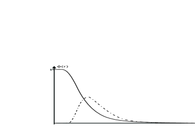
Figure 1: The radial defect $\phi(r)$ and the color charge density $\rho(r)$ (the dot-dashed line) for $D=3$ and $p=4$. The leading term of $\rho(r)$ in the asymptotic limit is $\sim 1/r^{6}$. The color charge is localized around the radius $R$ of the defect which approaches to its core for $p$ very large.

A color dielectric function $G$ for this case with the suitable behavior displayed in Eq. (14) can be given by

$$G(\phi)=\left[\frac{\phi^{2}}{\phi^{2}+(A_{\alpha})^{l}(\phi^{\beta/p}+1)/2}\right]^{2\alpha},$$ (21)

where $l,\,\alpha>0$, $\beta<0$ and $A_{\alpha}=4\alpha-1$. Now, we substitute Eq. (18) in the limit of large $p,$ and we use Eqs. (20) and (21) into (8) to find

$$r^{2}\left\{\frac{1}{1+(A_{\alpha})^{l}[(rp)^{-\beta+2p}+(rp)^{2p}]/2}\right\}^{2\alpha}\frac{dU}{dr}$$

$$=\frac{q}{2}\frac{c(p)}{p}\left(\frac{1}{rp}\right)^{2p}.$$ (22)

In the case $2\alpha=1$ we take the leading term in $p$ to get

$$\frac{dU}{dr}=\frac{q}{4}\frac{c(p)}{p}\left(\frac{1}{r^{2}}+p^{-\beta}r^{-\beta-2}\right).$$ (23)

This is the color electric field in $D=3$ dimensions. The color electric potential obtained by integrating over the radial coordinate $r$ is

$$U(r)=\frac{q}{4}\frac{c(p)}{p}\left[-\frac{1}{r}+f_{\beta}(r)\right].$$ (24)

The first term is the well-known Coulomb potential and the second term comprises the confining part of the potential. This part $f_{\beta}(r)$ can be given in several distinct forms: for $\beta=-1$ we obtain

$$f_{\beta}(r)=p\ln{r}.$$ (25)

On the other hand, for $\beta\neq-1$, we get the following formula

$$f_{\beta}(r)=-p^{-\beta}\,\frac{r^{-\beta-1}}{\beta+1}.$$ (26)

In this case we have, for $\beta=-3/2$, $f_{\beta}(r)\sim\sqrt{r}$, and this reproduces the confining part of the Motyka-Zalewski potential MZ ; Z ; for $\beta=-2$, $f_{\beta}(r)\sim{r}$, and now we get the well-known linear confining part of the Cornell potential; and for $\beta=-3$, $f_{\beta}(r)\sim{r^{2}}$. For $\beta>-1$ the potential does not confine. As we can see, in the linear regime the tension of the QCD string td ; willets is very strong and scales as $\sim p^{2}$.

III Electric, magnetic and dyonic defects

The electrically charged defects that we have found can be used to give rise to other solutions. To do this, let us now investigate the total energy of the global defect found in $D\!=\!3$ dimensions. It can be cast to the form mts

$$E_{e}=\int_{1/p}^{\infty}dr\;r^{2}\left[\frac{1}{2}\left(\frac{d\phi}{dr}\right)^{2}+\frac{Q_{e}^{2}}{2\,r^{4}\,G}+V\right],$$ (27)

where we integrate from $1/p,$ for $p$ very large, to conform with the approximation we have done for the charge density [see Eq. (20)], and with the size of the defect. In the above expression, the second term is the color electric contribution, $Q_{e}$ is the color electric charge of the defect and $G$ is the color dielectric function. The scalar potential with $W_{\phi}$ chosen as in Eq. (16), goes to zero as $p$ (even) becomes very large. In this limit our model approaches the model studied recently in Ref. slusa2 . In the limit of large $p$ the solution (18) and $G$ given as in Eq. (II.1) turn out to be

$$\phi(r) \simeq \left(\frac{1}{r\,p}\right)^{p},$$ (28)

$$G(\phi(r)) \simeq \left(\frac{1}{1+(A_{\alpha})^{l}\,r^{2p}\,p^{2p}}\right)^{2\alpha},$$ (29)

where $A_{\alpha}=4\alpha-1$ and $l$ are positive parameters of the approximated color dielectric function. Now, we substitute Eqs (28) and (29) into Eq. (27) to get to the energy

$$E_{e}=\frac{1}{2}\frac{(A_{\alpha})^{l/2p}\,p\,Q_{e}^{2}\,\Gamma{\left(-2\,\alpha+\frac{1}{2p}\right)}\,\Gamma{\left(-\frac{1}{2p}\right)}}{2p\,\Gamma{(-2\,\alpha)}}.$$ (30)

Since the parameter $p$ is assumed to be very large, the formula above provides a simple expression for the energy which is given by $E_{e}=-\frac{1}{2}(A_{\alpha})^{l/2p}\,p\,Q_{e}^{2}$. Notice that the energy is very large because $p$ is very large.

The above result can be extended to magnetic solutions. Differently of the lines followed by Ref. slusa2 , here we do not consider the Wu-Yang SU(2) magnetic monopole solution of the non-Abelian sector of the theory; instead, we keep dealing with the Abelian sector and we assume that the global defect that we have found in $D\!=\!3$ is charged by a total magnetic charge $Q_{m}$. We make use of the results for the electric case to get the magnetic energy

$$E_{m}=\frac{1}{2}\frac{(A_{\alpha})^{l/2p}\,p\,Q_{m}^{2}\,\Gamma{\left(2\,\alpha+\frac{1}{2p}\right)}\,\Gamma{\left(-\frac{1}{2p}\right)}}{2p\,\Gamma{(2\,\alpha)}}.$$ (31)

The magnetic energy is easily found by making the transformation $Q_{e}\to Q_{m}$ and $G\to 1/G$ into Eq. (27) — see mts for details. As in the electric case, for large $p$, the magnetic energy tends to be of the form $E_{m}=-\frac{1}{2}(A_{\alpha})^{l/2p}\,p\,Q_{m}^{2}$. Notice that we are changing the dielectric function to a “magnetic permeability.” According to (29), we see that this transformation is equivalent to the change $\alpha\to-\alpha$. We can refer to the two charged defects as “electric defect” and “magnetic defect”, respectively.

The above electric and magnetic structures may be used to ask for the presence of “dyonic” configurations. As one knows, a dyon is an object with both electric and magnetic charges. Thus, let us consider the possibility of a dyonic structure with mass

$$M_{D}=|E_{e}+E_{m}|\leq|E_{e}|+|E_{m}|=M_{e}+M_{m}.$$ (32)

The stability of the dyonic object would be ensured by the inequality $M_{D}<M_{e}+M_{m}$. In supersymmetric theories the dyon is a BPS state whose mass is related to the central charge of the supersymmetric algebra. The stability of such BPS state depends crucially on the value of its parameters sbwit . Thus, in our case we can think of a similar way of getting stability of the dyon state with mass $M_{D}$. To do this, we see that for a suitable value of the parameter $l$ the energy of the magnetic defect (31) becomes imaginary. In this way, the sum $E_{e}+E_{m}$ produce a vector in the complex plane and then $M_{D}$ is the length of this vector whose magnitude is lesser than the sum of its components. Alternatively, for $l/2p$ being a semi-integer, and for $\alpha\to-\alpha$, $(A_{\alpha})^{l/2p}\to i(\tilde{A}_{\alpha})^{l/2p},$ (with $\tilde{A}_{\alpha}=|4\alpha+1|$) we get $E_{m}\to i\tilde{E}_{m}$. In this case $M_{D}$ is given by the formula

$$M_{D}=\sqrt{E_{e}^{2}+\tilde{E}_{m}^{2}}=\frac{1}{2}p\sqrt{q_{e}^{2}+q_{m}^{2}},$$ (33)

where the charges $q_{e}$ and $q_{m}$ are defined in terms of $E_{e}$ and $E_{m}$ in the limit of very large $p$ as

$$q_{e}=(A_{\alpha})^{l/2p}\,Q_{e}^{2},$$ (34)

$$q_{m}=(\tilde{A}_{\alpha})^{l/2p}\,Q_{m}^{2},$$ (35)

We notice that $q_{e}\leftrightarrow q_{m}$ as long as $\alpha\leftrightarrow-\alpha$ and $G\leftrightarrow 1/G$.

IV Comments and Conclusions

We summarize this work recalling that we have studied how the presence of new global defect structures could act to confine in an simplified, Abelian model where the scalar field self-interacts nontrivially, responding for changing the dielectric properties of the medium. To make the model more realistic, we have added fermions, which interact with the scalar field through an Yukawa coupling, similar to couplings required in a supersymmetric environment.

We have investigated a model in $D\!=\!3$ spatial dimensions that seems to respond to confinement very appropriately. Similar investigations can perfectly be addressed in any $D$ spatial dimensions. In particular, in $D\!=\!1$ we could use the superpotential (16) for $p\!=\!3,5,...,$ which was shown to give rise to defect solutions of the form of 2-kink solutions bmm , which the kinks separated by a distance which increases with increasing $p\!=\!3,5,...$ This feature has been further explored in Ref. bfg , where one couples the model to gravity in $(4,1)$ spacetime dimensions in warped spacetime with one extra dimension. There one also finds results which highlight the fact that the superpotential (16) gives rise to 2-kink defect structures for $p\!=\!3,5,...$ These solutions could be used in the present context, to investigate confinement with these 2-kink defects. Investigations on this appear interesting because it could offer an alternative to Ref. bbf101 , using a simpler model which requires a single real scalar field to generate 2-kink structures.

In $D\!=\!3$ dimensions, we have shown that the monopole-like, electrically charged global defect can be used to generate magnetically charged global defect. This is implemented by essentially changing the “color” dielectric function $G(\phi)$ to its inverse $1/G(\phi).$ This feature has inspired us to search for dyons, for dyonic-like structures which should be stable bound states of electrically and magnetically charged global defects, whose mass should be given in terms of the electric and magnetic charges.

- (1) E. Eichten ., Phys. Rev. Lett. 34, 369 (1975).
- (2) L. Motyka and K. Zalewski, Z. Phys. C 69, 342 (1996).
- (3) K. Zalewski, Acta Phys. Pol. B 29, 2535 (1998).
- (4) M. Ślusarczyk and A. Wereszczyński, Eur. Phys. J. C 23, 145 (2002).
- (5) L. Wilets, Nontopological solitons (World Scientific, Singapore, 1989).
- (6) A. Chodos, R.L. Jaffe, K. Jonhson, C.B. Thorn and V.F. Weisskopf, Phys. Rev. D 9, 3471 (1974).
- (7) W.A. Bardeen, M.S. Chanowitz, S.D. Drell, M. Weinstein and T.-M. Yan, Phys. Rev. D 11, 1094 (1975).
- (8) R. Friedberg and T.D. Lee, Phys. Rev. D 15, 1964 (1977).
- (9) R. Dick, Phys. Lett. B 397, 193 (1997).
- (10) R. Dick, Phys. Lett. B 409, 321 (1997).
- (11) R. Dick, Eur.Phys.J. C 6, 701 (1999).
- (12) S. Mandelstam, Phys. Rep. 23C, 145 (1976); G. ’t Hooft, in Proceed. of Euro. Phys. Soc. 1975, ed. A. Zichichi.
- (13) N. Seiberg and E. Witten, Nucl. Phys. B426, 19 (1994).
- (14) V. Singh, D.A. Browne and R.W. Haymaker, Phys. Lett. B306, 115 (1993).
- (15) A similar procedure to construct an effective Lagrangian by substituting solutions of equation of motion into the original Lagrangian has been considered, e.g., in Ref. olum .
- (16) D. Bazeia, J. Menezes and R. Menezes, Phys. Rev. Lett. 91, 241601 (2003).
- (17) E. Witten, Nucl. Phys. B 507, 658 (1997).
- (18) M.A.C. Kneipp and P. Brockill, Phys.Rev. D64, 125012 (2001).
- (19) D. Bazeia, F.A. Brito, W. Freire and R.F. Ribeiro, Int. J. Mod. Phys. A18, 5627 (2003).
- (20) C. Montonen and D. Olive, Phys. Lett. B 72, 117 (1977).
- (21) R. Hobard, Proc. Phys. Soc. Lond. 82, 201 (1963).
- (22) G.H. Derrick, J. Math. Phys. 5, 1252 (1964).
- (23) R. Jackiw, Rev. Mod. Phys. 49, 681 (1977).
- (24) T.D. Lee, Particles physics and introduction to field theory (Harwood Academic, New York, 1981).
- (25) M. Rosina, A. Schuh and H.J. Pirner, Nucl. Phys. A 448, 557 (1986).
- (26) Ch. Schlichter, G. S. Bali, K. Schilling, Nucl. Phys. Proc. Suppl. 63, 519 (1998).
- (27) G. ’t Hooft, Nucl. Phys. B190, 455 (1981).
- (28) A.S. Kronfeld, M.L. Laursen, G. Schierholz, U.J. Wiese, Phys. Lett. B198, 516 (1987).
- (29) H. Shiba et al., Phys. Lett. B333, 461 (1994).
- (30) G.S. Bali et al., Phys. Rev. D54, 2863 (1996).
- (31) M. Chabab, R. Markazi, and E.H. Saidi, Eur. Phys. J. C 13, 543 (2000).
- (32) M. Chabab, N. El Biaze, R. Markazi, and E.H. Saidi, Class. Quant. Grav. 18, 5085 (2001).
- (33) M. Cvetič and A.A. Tseytlin, Nucl. Phys. B 416, 137 (1994).
- (34) M. Salem and T. Vachaspati, Phys. Rev. D 66, 025003 (2002).
- (35) K.D. Olum and N. Graham, Phys. Lett. B554, 175 (2003); N. Graham and K.D. Olum, Phys. Rev. D 67, 085014 (2003).
- (36) R. Jackiw and C. Rebbi, Phys. Rev. D 13, 3398 (1976).
- (37) V. Villalba, J. Math. Phys. 36, 3332 (1995).
- (38) F.A. Brito and D. Bazeia, Phys. Rev. D 56, 7869 (1997).
- (39) D. Bazeia, H. Boschi-Filho and F.A. Brito, J. High Energy Phys. 04, 028 (1999).
- (40) D. Bazeia and F.A. Brito, Phys. Rev. D 61, 105019 (2000)
- (41) A. Wereszczyński and M. Ślusarczyk, Eur. Phys. J. C30, 537 (2003).
- (42) D. Bazeia, C. Furtado, and A.R. Gomes, J. Cosmol. Astropart. Phys. 02, 002 (2004).