Late cosmology of brane gases with a two-form field

Abstract

We consider the effects of a two-form field on the late-time dynamics of brane gas cosmologies. Assuming thermal equilibrium of winding states, we find that the presence of a form field allows a late stage of expansion of the Universe even when the winding degrees of freedom decay into a pressureless gas of string loops. Finally, we suggest to understand the dimensionality of the Universe not as a result of the thermal equilibrium condition but rather as a consequence of the symmetries of the geometry.

Brane gas cosmology Alexander et al. (2000) is a scenario inspired by string theory which gives an appealing resolution to the initial singularity problem of the standard cosmological model and proposes a dynamical explanation for the number of spatial dimensions of the Universe. In this type of string cosmologies the geometry of the early Universe is described by a $D+1$-dimensional spacetime with a spatial toroidal section and the dynamics is assumed to be driven by a gas containing all the extended degrees of freedom, or Dp-branes Polchinski (1998), that the spectrum of a particular string theory could admit. This scenario is, in fact, a natural extension of the original proposal which considers a Universe filled with a gas of fundamental strings. Brandenberger and Vafa (1989); Tseytlin and Vafa (1992); Tseytlin (1992a) (see Bassett et al. (2003) for a recent discussion of some cosmological implications).

The fundamental string/brane states in the gas are the winding modes, the momentum modes, and the oscillatory modes. This spectrum is invariant under the inversion of the radius of the torus –a symmetry which is called T duality and interchanges winding a momentum modes. In the basic picture the spacetime starts small, namely with a typical size of the order of the string length, at the Hagedorn temperature. As the Universe grows the energy of winding modes increases leading to a confining potential that prevents further expansion. In the absence of equilibrium these modes cannot decay and the Universe starts contracting. As the size decreases the energy of the momentum modes becomes important. Then, the contraction phase is stopped and the Universe is prevented from reaching a zero size. The role of both types of modes is dual: winding modes stop expansion whereas momentum modes stop contraction. Without a mechanism to get rid of winding modes all the spatial dimensions of the Universe would oscillate around the string length scale. Nevertheless, if thermal equilibrium is maintained, and an adiabatic evolution is assumed so that the expansion rate is smaller than the interaction rate, energy from the winding states can be transferred to the rest of the states of the spectrum and, thus, the universe can be kept expanding. By considering the probability of intersection of the worldvolume of two Dp-branes, it follows that the annihilation mechanism can take place only if the largest dimensionality of the spacetime is $2p+2$. Modes with large $p$ are more massive and, consequently, must decay earlier than modes with lower $p$. Thus, the dimensionality of the space could be reduced successively creating a hierarchy of small dimensions. Since the last modes to be annihilated are those with $p=1$, there is no problem in having a large Universe expanding in three spatial dimensions. Different aspects of this scenario has been studied in Easson (2001); Easther et al. (2002); Brandenberger et al. (2002); Watson and Brandenberger (2003a); Boehm and Brandenberger (2003); Campos (2003); Easther et al. (2003); Alexander (2003); Kaya and Rador (2003); Kaya (2003); Biswas (2003); Watson and Brandenberger (2003b); Brandenberger et al. (2003)

The cosmology of brane gases has two shortcomings. First, causality implies that even with an efficient annihilation of winding states at least one Dp-brane across a Hubble volume should have survived. As with domain wall defects, this is incompatible with current experimental data of the fluctuations in the temperature of the microwave background radiation. A solution to this problem, proposed in Alexander et al. (2000) and further developed in Brandenberger et al. (2002) (see also Campos (2003)), is to invoke a sufficiently long period of cosmological loitering which might have allowed the whole spatial extent of the Universe to be in causal contact, so that the actual absence of branes can be explained by a microphysical process. The second problem with these scenarios is that they describe the very early stages of the Universe only, and a mechanism to connect this string theory regime to a late classical cosmological evolution is still needed. This is, in fact, connected with the problem of dilaton potential generation which is still not fully understood and is one of the most outstanding challenges for string theory.

In previous analysis of string/brane gas cosmology the effects of fluxes have been ignored and the background dynamics has been described by a gravitational field and a dilaton field only. The purpose of the present work is to investigated the importance of the Neveu-Schwarz–Neveu-Schwarz (NS-NS) sector on the evolution of this type of cosmologies. As we will see, the effects of fluxes can dominate over winding or unwinding degrees of freedom at late times and introduce significant modifications on the cosmological evolution of the Universe. As an immediate implication, we suggest to understand the number of spatial dimensions of the spacetime as a consequence of homogeneity.

The cosmological dynamics of this scenario is dictated by the bosonic action Alexander et al. (2000),

$$S_{B}=-\int d^{D+1}x\,\sqrt{-g}\,e^{-2\phi}\left[R+4(\nabla_{\mu}\phi)^{2}-\frac{1}{12}H^{2}_{\mu\nu\alpha}\right]\,,$$ (1)

which involves the dynamics of the metric tensor $g_{\mu\nu}$, a dilaton field $\phi$, and a two-form field $B_{\mu\nu}$ through its field strength $H_{\mu\nu\alpha}=3\nabla_{[\mu}B_{\nu\alpha]}$. (We employ units in which the string length is $l_{st}\sim 1$.) This low-energy effective action describes a type II superstring theory without a Ramond-Ramond sector and arises from the compactification of 11-dimensional supergravity on a circle. The dilaton field represents the radius of compactification and defines the string coupling, which is assumed to be small in order to ensure an effective compactification. The equations of motion derived from this action are,

$$R_{\mu\nu}+2\nabla_{\mu}\nabla_{\nu}\phi = \frac{1}{4}H_{\mu\alpha\beta}H^{\alpha\beta}{}_{\nu}$$

$$-\frac{e^{2\phi}}{\sqrt{-g}}\left(\frac{\delta S_{m}}{\delta g^{\mu\nu}}-\frac{1}{4}g_{\mu\nu}\frac{\delta S_{m}}{\delta\phi}\right)\,,$$

$$2\Box\phi-4(\nabla_{\mu}\phi)^{2} = -\frac{1}{6}H^{2}_{\mu\nu\alpha}$$

$$+\frac{e^{2\phi}}{\sqrt{-g}}\left(g^{\mu\nu}\frac{\delta S_{m}}{\delta g^{\mu\nu}}-\frac{D-1}{4}\frac{\delta S_{m}}{\delta\phi}\right)\,,$$

$$\nabla^{\mu}(e^{-2\phi}H_{\mu\nu\alpha}) = 0\,.$$

The gas of Dp-branes is represented by the matter action $S_{m}$. Since we are interested in analysing the late-time cosmological evolution, we will assume that all winding states with $p>1$ have already decayed and only modes with $p=1$ are still interacting in a expanding background with three spatial dimensions. Here we shall concentrate the analysis on spatially flat homogeneous and isotropic metrics,

$$ds^{2}=-N^{2}(t)dt^{2}+e^{2\lambda(t)}\sum^{3}_{i=1}dx^{2}_{i}\,.$$ (2)

We have kept the lapse function, $N(t)$, in order to facilitate a later rederivation of the full set of equations of motion. A solution to the above dynamical equations can be obtained by adopting the following ansatz for the field strength (see for instance Freund and Rubin (1980); Freund (1982); Tseytlin (1992b); Goldwirth and Perry (1994); Lidsey et al. (2000)),

$$H_{\mu\nu\alpha}=e^{2\phi}\epsilon_{\mu\nu\alpha\beta}\nabla^{\beta}h\,,$$ (3)

where $\epsilon_{\mu\nu\alpha\beta}$ is the totally antisymmetric covariantly conserved volume form. In addition, the field strength satisfies a closure condition, $\nabla_{[\beta}H_{\mu\nu\alpha]}=0$ (Bianchi identity), which follows from its definition in terms of an antisymmetric form field, that yields a differential equation for the scalar function $h$, $\nabla_{\mu}(e^{2\phi}\nabla^{\mu}h)=0$. A homogeneous solution to this equation, $h(t)$, can be easily obtained and leads to a field strength,

$$H^{2}_{\mu\nu\alpha}=6H^{2}_{o}e^{-6\lambda}\equiv 12U(\lambda)\,,$$ (4)

where $H_{o}$ is a constant of integration. Then, for the metric (2), the bosonic action (1) takes the following simple form,

$$S_{B}=-\int dt\,e^{-\varphi}\left[\frac{1}{N}(3\dot{\lambda}^{2}-\dot{\varphi}^{2})-NU(\lambda)\right]\,,$$ (5)

where the new ”shifted” dilaton field $\varphi\equiv 2\phi-3\lambda$ serves to absorb the space volume factor in the action. It is important to observe that the net effect of the form field is to yield an effective exponential potential for the scalar field $\lambda$. As we will see later this feature will have important consequences on the late cosmological dynamics.

By using the gauge $N(t)=1$, the equations of motion derived from the total effective action (bosonic plus matter sectors) can be written as Tseytlin and Vafa (1992); Tseytlin (1992a, b); Veneziano (1991); Gasperini and Veneziano (2003),

$$\dot{\varphi}^{2}-3\dot{\lambda}^{2} = e^{\varphi}E+U(\lambda)\,,$$ (6)

$$\ddot{\varphi}-3\dot{\lambda}^{2} = \frac{1}{2}\,e^{\varphi}E\,,$$ (7)

$$\ddot{\lambda}-\dot{\varphi}\dot{\lambda} = \frac{1}{2}\,e^{\varphi}P+U(\lambda)\,,$$ (8)

where $E$ and $P$ are the total energy and pressure build on all (winding and non-winding) matter source contributions,

$$E = E_{w}+E_{nw}\,,$$ (9)

$$P = P_{w}+P_{nw}\,.$$ (10)

The assumption of an adiabatic evolution of matter previously mentioned implies the conservation equation $\dot{E}+3\dot{\lambda}P=0$ Tseytlin and Vafa (1992). Note that this condition, together with Eqs. (7), (8), and (4), ensures that the energy constraint (6) is a conserved quantity. For the non-winding modes we consider an ordinary barotropic equation of state $P_{nw}=\gamma E_{nw}$ with $0\leq\gamma\leq 1$. This includes, for instance, the production of non-winding modes in the form of radiation ($\gamma=1/3$) or in the form of a pressureless fluid ($\gamma=0$). On the other hand, for the collective dynamics of winding modes we assume a typical equation of state $P_{w}=-E_{w}/3$ Alexander et al. (2000); Boehm and Brandenberger (2003); Vilenkin and Shellard (1994). It is important to point out that, in principle, one should expect a modification of this relation between the total winding energy and momentum when the dynamics of a form field is taking into account (simply because the effective action for individual branes depends explicitly on the field $B_{\mu\nu}$ induced on the worldvolume Polchinski (1998) (see also Leigh (1989))). However, we shall consider in our analysis that this is not a dominant effect on the full equation of state for the brane gas and, consequently, that the mass energy dominates over all other mode fluctuations. In fact, if the form field induced on the brane is viewed as a small deviation from the induced metric the corrections to the equations of motion will be of quadratic order. Then, although our assumption presents some limitations, it will give an accurate description as long as the field strength does not grow very large.

We shall first ignore the contribution of all matter sources and consider the case in which $E=P=0$. Then, Eqs. (6)-(8) have the following general solution,

$$\lambda(\eta)=\frac{\sqrt{3}}{6}(A\eta+B)+\frac{1}{2}\ln\left[\frac{H_{o}}{A}\cosh A(\eta-\eta_{o})\right]\,,$$ (11)

$$\varphi(\eta)=-\frac{\sqrt{3}}{2}(A\eta+B)-\frac{1}{2}\ln\left[\frac{H_{o}}{A}\cosh A(\eta-\eta_{o})\right]\,,$$ (12)

where the time parameter $\eta$ is defined by $dt=e^{-\varphi(\eta)}d\eta$. Here, $A$, $B$, and $\eta_{o}$ are constants of integration. An expression for cosmic time, $t$, in terms of $\eta$ can be computed analytically,

$$t(\eta) = \frac{(2H_{o})^{\frac{1}{2}}}{(\sqrt{3}-1)A^{\frac{3}{2}}}e^{\frac{\sqrt{3}}{2}(A\eta_{o}+B)}e^{\frac{\sqrt{3}-1}{2}A(\eta-\eta_{o})}$$ (13)

$$\times F\left(-\frac{1}{2},\frac{\sqrt{3}-1}{4};\frac{\sqrt{3}+3}{4};-e^{2A(\eta-\eta_{o})}\right)\,,$$

where $F$ is the hypergeometric function. At late times one has,

$$\eta\underset{t\rightarrow\infty}{\longrightarrow}\frac{2}{(\sqrt{3}+1)A}\ln t\,,$$ (14)

and then the universe expands asymptotically with a scale factor,

$$e^{\lambda(t)}\underset{t\rightarrow\infty}{\longrightarrow}t^{\sqrt{3}/3}\,.$$ (15)

However, the string coupling gets large,

$$g\equiv e^{\phi}\underset{t\rightarrow\infty}{\longrightarrow}t^{(\sqrt{3}-1)/2}\,,$$ (16)

and the theory becomes strongly coupled Mukherji (1997).

Turning back to the case in which the universe is driven by a gas of branes we first need to supplement the field equations (6)-(8) with an appropriate description of the decay of winding modes into states without winding number. For our analysis we will closely follow the discussion of Campos (2003). The self-interaction of winding modes can be thought as analogous to that of a network of long cosmic strings decaying into small string loops Bennett (1986a, b); Vilenkin and Shellard (1994); Brandenberger (1994) (For a detailed account of brane interactions in an expanding universe see also Majumdar and Davis (2003)). At time $t$ the total winding energy, $E_{w}$, and the total energy of the string loops (states without winding number) produced, $E_{l}$, can be expressed in general as,

$$E_{w}(t) = \tau l_{c}N_{w}(t)e^{\lambda(t)}\,,$$ (17)

$$E_{l}(t) = \tau l_{c}N_{l}(t)e^{-3\gamma\lambda(t)}\,,$$ (18)

where $N_{w}$ and $N_{l}$ represent the number of winding modes and small loops, respectively. $\tau$ is the tension corresponding to a D1-brane and $l_{c}$ is a derived length scale related with the initial size of the spatial dimensions of the torus $l_{c}\sim l_{st}\exp(-\lambda(0))$. The decrease of winding energy, due to the decay into small loops, can be roughly estimated to be proportional to the square of the number of winding modes Vilenkin and Shellard (1994),

$$\dot{E}_{w}\sim-c\,\tau N^{2}_{w}(t)\left(\frac{L_{l}(t)}{R(t)}\right)\,.$$ (19)

The parameter $c$ measures the efficiency of loop production and, correspondingly, it is zero if there is no winding mode annihilation. $L_{l}(t)$ represents the typical size of the loops created and it will be taken proportional to the cosmic time $t$ Bennett (1986b) (see also Brandenberger et al. (2002) and Campos (2003)). From Eq. (19) and within the adiabatic approximation we can find evolution equations for $N_{w}(t)$ and $N_{l}(t)$,

$$\dot{N}_{w}(t) = -\frac{c}{l^{2}_{c}}L_{l}(t)N^{2}_{w}(t)e^{-2\lambda(t)}\,,$$ (20)

$$\dot{N}_{l}(t) = \frac{c}{l^{2}_{c}}L_{l}(t)N^{2}_{w}(t)e^{(3\gamma-1)\lambda(t)}\,.$$ (21)

To keep the discussion simple we do not consider more elaborated annihilation processes such as those taking into account the reconnection of small loops or a subsequent loop decay into gravitational radiation. Finally, the field equations (6)-(8) can be transformed into a closed set of first-order differential equations by introducing the new variables $f=\dot{\varphi}$ and $l=\dot{\lambda}$,

$$\dot{f} = 3l^{2}+\frac{1}{2}\,e^{\varphi}\left(E_{w}+E_{l}\right)\,,$$ (22)

$$\dot{l} = fl-\frac{1}{6}\,e^{\varphi}\left(E_{w}-3\gamma E_{l}\right)+U(\lambda)\,,$$ (23)

$$f^{2} = 3l^{2}+e^{\varphi}\left(E_{w}+E_{l}\right)+U(\lambda)\,,$$ (24)

together with Eqs. (4), (17), (18), (20), and (21).

Let us comment on the general properties of the above dynamical equations. The straight lines $l=\pm f/\sqrt{3}$ are solutions with $E_{w}=E_{l}=U=0$. Since $U(\lambda)$ is nonnegative, the region with $f^{2}-3l^{2}<0$ represents configurations with a negative total matter energy and therefore it is excluded from the analysis (see Fig. 1). On the other hand, Eq. (22) implies that $\dot{f}>0$ and then $f$ is always growing. If initially $f$ is negative it will approach zero asymptotically and $\varphi$ will be a decreasing function of time. For those trajectories that obey the condition $f-3l<0$, the dilaton is also decreasing and thus one can be certain that the weak coupling condition is enforced Campos (2003). The evolution of the variable $l$ (the Hubble function) is dictated by Eq. (23) which has a simple mechanical interpretation: it describes the classical motion of a damped particle in a time-dependent potential, which in our case is given by

$$\tilde{U}(\lambda) = \frac{\tau l_{c}}{6}\,e^{\varphi}\left[N_{w}(t)\,e^{\lambda}+N_{l}(t)\,e^{-3\gamma\lambda}\right]+\frac{1}{6}U(\lambda)$$

$$= \frac{\tau l_{c}}{6}\,e^{\varphi}\left[N_{w}(t)\,e^{\lambda}+N_{l}(t)\,e^{-3\gamma\lambda}+\frac{H^{2}_{o}e^{-\varphi}}{2\tau l_{c}}\,e^{-6\lambda}\right].$$

The analysis of this effective potential gives a valuable information of the full dynamics. First, consider the flux is negligible ($H_{o}=0$) and the gas of branes is out of thermal equilibrium. Then, $N_{l}=0$ and $N_{w}$ is approximately constant. This situation leads to an oscillating cosmological evolution. If the Universe is growing the winding term dominates and tends to stop the expansion. On the other hand, when it is contracting the momentum modes become important and causes the Universe to reexpand. (These modes can be roughly represented by a potential similar to the second term with $\gamma=1/3$ and $N_{l}$ a non vanishing constant.) This behaviour, which typically describes the dynamics close to the Hagedorn temperature Brandenberger and Vafa (1989), changes once thermal equilibrium has been established. Now winding energy can be transfered to matter energy and the second term starts to dominate as $N_{l}$ increases and $N_{w}$ decreases. Under these conditions, the Universe can pass through a contraction phase, the longer the less efficient the energy transfer is, but it shall inevitably expand in the future. Nevertheless, as it was shown in Campos (2003), if winding modes decay into a pressureless gas ($\gamma=0$) of small string loops, (LABEL:eq:clas_pot) always represents a confining potential and the Universe cannot expand and grow large. As a consequence, the dimensionality of the spacetime cannot be explained by this mechanism in this particular case.

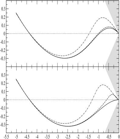
Figure 1: Phase space $(f,l)$. These curves represent the numerical solutions of the equations of motion for an efficiency parameter of the winding mode decay $c=0.1$, and a gas of small loops with $\gamma=1/3$ (top) and $\gamma=0$ (bottom). The straight lines correspond to $H_{o}=0$, the dashed lines to $H_{o}=0.001$, and the dotted-dashed lines to $H_{o}=0.005$. The grey area, $f^{2}-3l^{2}<0$, represents a region where the total matter energy is negative. The border lines, $l=\pm f/\sqrt{3}$, are straight solutions with $E_{w}=E_{l}=U=0$ and therefore cannot be crossed by other trajectories.

The importance of the two-form field contribution, on the other hand, is more difficult to assess without solving the equations of motion, because it also involves the dynamics of the field $\varphi$. Naively, one should expect that the last term in the effective potential (LABEL:eq:clas_pot) could dominate the dynamics only if $\varphi$ becomes negatively large. In Fig. 1 the numerical solution of the full set of dynamical equations has been plotted for different parameters of the model. As one can observe, the contribution from the flux is only significant at late times. When the small loops are produced in the form of a gas with $0<\gamma\leq 1/3$ (in Fig. 1 the case of a gas of radiation, $\gamma=1/3$, has been plotted), the cosmological evolution do not change qualitatively. Mainly, the effect of the two-form field is to reduce the rate of contraction and increase the rate of late expansion. However, if the loops produced behave as ordinary static matter with zero pressure, $\gamma=0$, the qualitative change is much more interesting. In this case, contrary to what happens when there is no flux field (the case $H_{o}=0$ in Fig. 1), the Universe is able to escape from the contraction phase induced by the winding mode potential and finally reexpands. This behaviour overcomes the obstruction for explaining the dimensionality of the spacetime previously mentioned for a pressureless gas of string loops. In Campos (2003), another mechanism was proposed to solve this problem by considering the dynamics of a gas of nonstatic branes. In this case, the equation of state for the gas depends explicitly on a constant characteristic average velocity that modifies qualitatively the cosmological role of winding modes. For values of this velocity above certain threshold, the winding potential is no longer a confining potential. Thus winding modes do not tend to stop expansion and the universe cannot enter a phase of contraction. The problem with this mechanism is that the assumption of a time independent average velocity is likely very strong and, unfortunately, a clear picture of its time evolution is still needed.

To sum up, we see that under thermal equilibrium the dynamics of a flux field dominates at late times over the nonwinding degrees of freedom. The next obvious question to ask is whether the form field term in the effective potential also dominates if there is no winding mode decay. This would immediately imply that the confining potential of the winding states will not be able to stop the expansion of the Universe, and consequently, one could question if the assumption of thermal equilibrium is essential in order to explain the dimensionality of the spacetime. To investigate this issue we have solved the equations of motion considering that the winding modes are not annihilated by self-interactions. As can be seen from Fig. 2 the early dynamics is dominated by the winding modes that try to halt the Universe but, at some point in the evolution, the flux field catches up and then triggers a late phase of expansion. Thus, in principle, when fluxes are taking into account one can relax the thermal equilibrium condition and still be able to have a Universe with three large spatial directions. Once the Universe gets out of the string regime and enters a classical evolution, the decay (for instance, in the form of radiation) of winding modes, and therefore thermal equilibrium, will eventually be required to avoid an undesirable future expanding evolution because the energy density of these modes would dominate over other forms of matter.

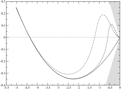
Figure 2: Phase space $(f,l)$. These curves represent the numerical solution of the equations of motion without winding mode annihilation ($c=0$). The straight line correspond to $H_{o}=0$, the dashed line to $H_{o}=0.001$, and the dotted-dashed line to $H_{o}=0.005$.

What we would like to stress is the possibility that thermal equilibrium could not be a fundamental prerequisite for explaining the number of space dimensions of the Universe. Instead, we suggest that it is the symmetry imposed on the geometry the assumption which is essential. The most simple picture one can think of is that of a homogeneous and isotropic Universe with $D+1$ small spacetime dimensions in a initial state consisting of a flux field, and winding and momentum degrees of freedom not necessarily in thermal equilibrium. The existence of a spatially homogeneous three-form field strength is compatible with a homogeneous and isotropic spacetime only in two (electric solution) or three (magnetic solution) spatial dimensions Lidsey et al. (2000) which implies that the flux has to live in a submanifold of the full spacetime. One can think of this lower dimensional subspace as a D2- or D3-brane carrying some charge. For the electric solution the field strength contributes to the effective potential (LABEL:eq:clas_pot) with a confining term of the form $e^{6\lambda}$, thus the Universe will always oscillate and remain small. For the magnetic solution, nevertheless, the situation is quite different. To begin with, consider the Universe is initially in an expansion stage driven by momentum modes. As the Universe grows, the winding energy will start to dominate and oppose the expansion. Then, the Universe can start contracting in all its spatial directions. This goes on until the field strength contribution builds up and the contraction is reversed in the submanifold containing the flux field. The expansion of this subspace cannot be stopped by winding modes and then a 3+1-dimensional Universe can grow large. The rest of the spatial directions will continue contracting and expanding indefinitely but they will remain small. In that sense it is fundamental for the stability of this internal space that the winding modes are out of thermal equilibrium. In this set up, the initial singularity is also avoided due to the presence of momentum modes that oppose contraction as the Universe becomes small. Furthermore, it offers an explanation for the precise number of spatial dimensions unlike the original proposal Brandenberger and Vafa (1989) which only provides an upper bound. It is worth emphasing that all these arguments can be easily generalised to an anisotropic picture.

In conclusion, we have studied the late cosmological evolution of a gas of branes by incorporating the dynamics of the NS-NS sector. We have shown that fluxes can dominate the dynamics of the Universe at late times and introduce significant effects. Assuming thermal equilibrium, these effects can account for a late stage of expansion even if the winding modes decay into a pressureless gas of string loops. Finally, we have argued that assuming homogeneity of the background the presence of a two-form field can easily explain the exact number of spatial dimensions of the Universe and the stability of the small internal space without requiring the decay of winding modes. This could mean that the fundamental assumption for understanding the dimensionality of the spacetime is the symmetry of the geometry and not the condition of thermal equilibrium of the winding states.

The author acknowledges the support of the Alexander von Humboldt Stiftung/Foundation and the Universität Heidelberg.

References

- Alexander et al. (2000) S. Alexander, R. H. Brandenberger, and D. Easson, Phys. Rev. D62, 103509 (2000).
- Polchinski (1998) J. Polchinski, String Theory (Cambridge University Press, Cambridge, England, 1998).
- Brandenberger and Vafa (1989) R. H. Brandenberger and C. Vafa, Nucl. Phys. B316, 391 (1989).
- Tseytlin and Vafa (1992) A. A. Tseytlin and C. Vafa, Nucl. Phys. B372, 443 (1992).
- Tseytlin (1992a) A. A. Tseytlin, Class. Quantum Grav. 9, 979 (1992a).
- Bassett et al. (2003) B. A. Bassett, M. Borunda, M. Serone, and S. Tsujikawa, Phys. Rev. D67, 123506 (2003).
- Easson (2001) D. A. Easson (2001), eprint hep-th/0110225.
- Easther et al. (2002) R. Easther, B. R. Greene, and M. G. Jackson, Phys. Rev. D66, 023502 (2002).
- Brandenberger et al. (2002) R. Brandenberger, D. A. Easson, and D. Kimberly, Nucl. Phys. B623, 421 (2002).
- Watson and Brandenberger (2003a) S. Watson and R. H. Brandenberger, Phys. Rev. D67, 043510 (2003a).
- Boehm and Brandenberger (2003) T. Boehm and R. Brandenberger, J. Cosmol. Astropart. Phys. 06, 008 (2003).
- Campos (2003) A. Campos, Phys. Rev. D68, 1040XX (2003), eprint hep-th/0304216.
- Easther et al. (2003) R. Easther, B. R. Greene, M. G. Jackson, and D. Kabat, Phys. Rev. D67, 123501 (2003).
- Alexander (2003) S. H. S. Alexander, J. High Energy Phys. 10, 013 (2003).
- Kaya and Rador (2003) A. Kaya and T. Rador, Phys. Lett. B565, 19 (2003).
- Kaya (2003) A. Kaya, Class. Quant. Grav. 20, 4533 (2003).
- Biswas (2003) T. Biswas (2003), eprint hep-th/0311076.
- Watson and Brandenberger (2003b) S. Watson and R. Brandenberger (2003b), eprint hep-th/0307044.
- Brandenberger et al. (2003) R. Brandenberger, D. A. Easson, and A. Mazumdar (2003), eprint hep-th/0307043.
- Freund and Rubin (1980) P. G. O. Freund and M. A. Rubin, Phys. Lett. B97, 233 (1980).
- Freund (1982) P. G. O. Freund, Nucl. Phys. B209, 146 (1982).
- Tseytlin (1992b) A. A. Tseytlin, Int. J. Mod. Phys. D1, 223 (1992b).
- Goldwirth and Perry (1994) D. S. Goldwirth and M. J. Perry, Phys. Rev. D49, 5019 (1994).
- Lidsey et al. (2000) J. E. Lidsey, D. Wands, and E. J. Copeland, Phys. Rep. 337, 343 (2000).
- Veneziano (1991) G. Veneziano, Phys. Lett. B265, 287 (1991).
- Gasperini and Veneziano (2003) M. Gasperini and G. Veneziano, Phys. Rep. 373, 1 (2003).
- Vilenkin and Shellard (1994) A. Vilenkin and E. P. S. Shellard, Cosmic String and Other Topological Tefects (Cambridge University Press, Cambridge, England, 1994).
- Leigh (1989) R. G. Leigh, Mod. Phys. Lett. A4, 2767 (1989).
- Mukherji (1997) S. Mukherji, Mod. Phys. Lett. A12, 639 (1997).
- Bennett (1986a) D. P. Bennett, Phys. Rev. D33, 872 (1986a).
- Bennett (1986b) D. P. Bennett, Phys. Rev. D34, 3592 (1986b).
- Brandenberger (1994) R. H. Brandenberger, Int. J. Mod. Phys. A9, 2117 (1994).
- Majumdar and Davis (2003) M. Majumdar and A.-C. Davis (2003), eprint hep-th/0304153.