Anomalous Magnetic Moment of Electron in Chern-Simons QED

Abstract

We calculate the anomalous magnetic moment of the electron in the Chern-Simons theory in $2+1$ dimensions with and without a Maxwell term, both at zero temperature as well as at finite temperature. In the case of the Maxwell-Chern-Simons (MCS) theory, we find that there is an infrared divergence, both at zero as well as at finite temperature, when the tree level Chern-Simons term vanishes, which suggests that a Chern-Simons term is essential in such theories. At high temperature, the thermal correction in the MCS theory behaves as $\frac{1}{\beta}\ln\beta M$, where $\beta$ denotes the inverse temperature and $M$, the Chern-Simons coefficient. On the other hand, we find no thermal correction to the anomalous magnetic moment in the pure Chern-Simons (CS) theory.

1 Introduction

Chern-Simons theories [1, 2] in $2+1$ dimensions have been of interest from a variety of reasons and have led to many interesting phenomena in various branches of physics [3]. In this paper, we systematically study the question of the anomalous magnetic moment of an electron in the Chern-Simons theory with and without a Maxwell term, both at zero as well as at finite temperature. In an Abelian theory, the magnetic moment is a gauge invariant quantity much like the Chern-Simons coefficient. As a result, its value is not related by the Ward identity to any other amplitude in the theory and needs to be studied independently. Our study brings out some new and interesting properties of Chern-Simons theories. For example, although conventionally one argues that the topological Chern-Simons term is an additional gauge invariant term that can be added to the action, the study of the anomalous magnetic moment, both at zero as well as finite temperature, reveals that such a term is, in fact, essential and in the absence of this term, physical quantities such as the magnetic moment cannot be defined because of infrared divergence. This has to be contrasted with the magnetic moment in $3+1$ dimensions where it is both ultraviolet and infrared finite. Normally, one expects infrared divergence to be more severe in lower dimensions. However, in $2+1$ dimensions it is believed that at least the Abelian theory has a well defined infrared behavior [4], unless one is at high temperature [5] and at higher loops [6]. Non-Abelian theories, of course, can have stronger infrared divergent behavior [7]. Our result, on the other hand shows that the Abelian theory can also exhibit infrared divergence at zero temperature at one loop in physical quantities, such as the anomalous magnetic moment unless there is a tree level Chern-Simons mass.

In $3+1$ dimensional QED, anomalous magnetic moment at zero temperature is one of the most intensively studied quantities both theoretically and experimentally where the value of $(g-2)$ is quite small [8]. In contrast, we find that in $2+1$ dimensions, the value of $(g-2)$ can become arbitrarily large depending on the value of the Chern-Simons coefficient. The thermal behavior of the anomalous magnetic moment in $3+1$ dimensions has also been studied [9, 10] and the temperature dependence determined to be $\frac{1}{\beta^{2}}$ at high temperatures, where $\beta$ denotes the inverse temperature. In $2+1$ dimensional Maxwell-Chern-Simons theory, we find that the thermal correction to the anomalous magnetic moment goes as $\frac{1}{\beta}\ln\beta M$ where $M$ represents the Chern-Simons coefficient. Furthermore, in the pure Chern-Simons theory, the anomalous magnetic moment surprisingly has no thermal correction.

The anomalous magnetic moment in $2+1$ dimensions has been studied earlier at zero temperature at one loop and the explicit value obtained in the large $M$ limit (anyonic limit or the pure CS limit) using the covariant Landau gauge [11]. Subsequently, this result has also been derived from a calculation in the pure Chern-Simons theory in the Coulomb gauge [12]. Our study, on the other hand, represents a complete systematic analysis of the anomalous magnetic moment at one loop in Chern-Simons theories with and without the Maxwell term, both at zero as well as at finite temperature. Our presentation is organized as follows. In section 2, we analyze the question of the anomalous magnetic moment in the MCS theory at zero temperature for an arbitrary value of the Chern-Simons coefficient which brings out the problem of the infrared divergence. Taking the large $M$ limit, we then obtain the known result for the pure CS theory [11, 12]. In section 3, we present our analysis of the finite temperature behavior of the anomalous magnetic moment. Here, the analysis for the MCS theory and the pure CS theory need to be done separately as we explain in the text. While the anomalous magnetic moment in the MCS theory behaves as $\frac{1}{\beta}\ln\beta M$ at high temperature, surprisingly there is no thermal correction to the anomalous magnetic moment in the pure CS theory. We speculate on the reason for such a behavior and conclude with a brief summary in section 4.

2 Zero Temperature

Let us consider the Maxwell-Chern-Simons theory described by the Lagrangian density

$${\cal L}=-\frac{1}{4}F_{\mu\nu}F^{\mu\nu}\pm\frac{M}{4}\epsilon^{\mu\nu\lambda}A_{\mu}F_{\nu\lambda}+\overline{\psi}(i\partial\!\!\!/-eA\!\!\!/-m)\psi-\frac{1}{2\xi}(\partial_{\mu}A^{\mu})^{2}+\partial^{\mu}\overline{c}\partial_{\mu}c\,.$$ (1)

Here $\xi$ represents the gauge fixing parameter and we have allowed for both signs of the Chern-Simons term. We assume that both the fermion mass as well as the Chern-Simons coefficient $(m,M)$ are nonnegative and define for later convenience their ratio to be

$$\kappa=\frac{M}{m}\geq 0\,,$$ (2)

which is a dimensionless constant. In the general covariant gauge, the photon propagator is given by

$$iD_{\mu\nu}(p)=-\frac{i}{p^{2}-M^{2}}\left(\eta_{\mu\nu}-\frac{p_{\mu}p_{\nu}}{p^{2}}\pm iM\epsilon_{\mu\nu\lambda}\frac{p^{\lambda}}{p^{2}}\right)-i\xi\,\frac{p_{\mu}p_{\nu}}{(p^{2})^{2}}\,,$$ (3)

while the fermion propagator has the form (the $i\epsilon$ prescription is understood)

$$iS(p)=\frac{i}{p\!\!\!/-m}=\frac{i(p\!\!\!/+m)}{p^{2}-m^{2}}\,.$$ (4)

We use the metric with signatures $(+,-,-)$ and a representation for the gamma matrices with $\gamma^{0}$ Hermitian, $\gamma^{i},i=1,2$ anti-Hermitian and satisfying

$$\gamma^{\mu}\gamma^{\nu}=\eta^{\mu\nu}-i\epsilon^{\mu\nu\lambda}\gamma_{\lambda}\,.$$ (5)

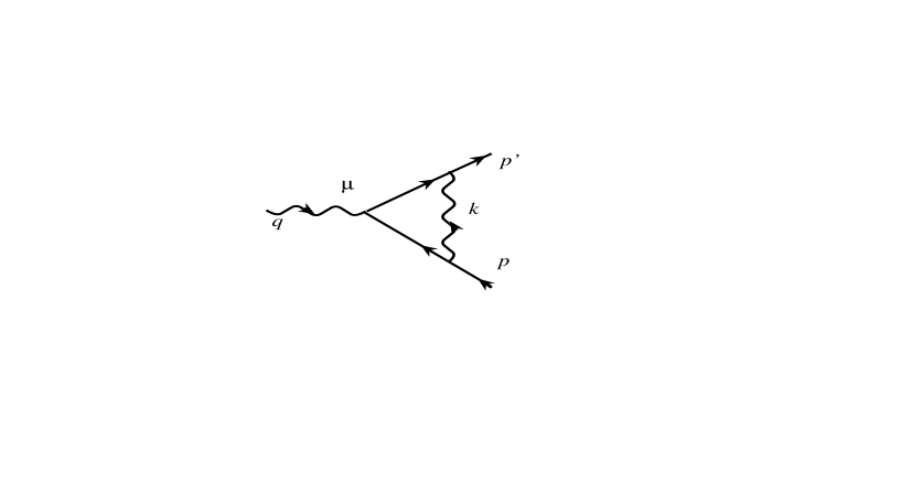
Figure 1: One-loop vertex correction.

The one loop correction to the vertex has the form

$$\Gamma^{\mu}(p,p^{\prime}) = (-ie)^{3}\int\mathrm{d}K\,\gamma^{\lambda}iS(p^{\prime}-k)\gamma^{\mu}iS(p-k)\gamma^{\rho}iD_{\rho\lambda}(k)$$ (6)

$$= e^{3}\int\mathrm{d}K\,\gamma^{\lambda}(p^{\prime}\!\!\!\!/-k\!\!\!/+m)\gamma^{\mu}(p\!\!\!/-k\!\!\!/+m)\gamma^{\rho}D_{\rho\lambda}(k)\times\frac{1}{k^{2}-2k\cdot p}\frac{1}{k^{2}-2k\cdot p^{\prime}}\,,$$

where $k$ is the internal loop momentum, $q$ the momentum transfer and we are assuming that the external fermions are on-shell so that

$$q^{\mu}=p^{\prime\mu}-p^{\mu},\quad p^{2}=p^{\prime 2}=m^{2},\quad{\rm and}\quad\mathrm{d}K=\frac{\mathrm{d}^{3}k}{(2\pi)^{3}}\,.$$ (7)

At zero temperature, the vertex function can be parameterized as

$$\Gamma^{\mu}(p,p^{\prime})=e\gamma^{\mu}\,F_{1}(q^{2})+\frac{ie}{4m}\,\left[\gamma^{\mu},q\!\!\!/\right]\,F_{2}(q^{2})=e\gamma^{\mu}\,F_{1}(q^{2})+\frac{e}{2m}\,\sigma^{\mu\nu}q_{\nu}\,F_{2}(q^{2})\,,$$ (8)

and the anomalous magnetic moment of the electron can be identified with $F_{2}(q^{2}=0)$.

The photon propagator in (3) (and, therefore in (6)) has a complex tensor structure compared to usual QED. First, let us show that the $p_{\mu}p_{\nu}$ terms in the photon propagator contribute only to the charge renormalization ($F_{1}(q^{2})$) and not to the magnetic moment. Replacing $D_{\rho\lambda}(k)\sim k_{\rho}k_{\lambda}$, the numerator in (6) takes the form

$$k\!\!\!/(p^{\prime}\!\!\!\!/-k\!\!\!/+m)\gamma^{\mu}(p\!\!\!/-k\!\!\!/+m)k\!\!\!/=\left((k^{2})^{2}-2k\cdot(p^{\prime}+p)k^{2}+4k\cdot p^{\prime}k\cdot p\right)\gamma^{\mu}\,,$$ (9)

which makes it clear that this can only contribute to the charge renormalization ($F_{1}(q^{2})$) and not to the magnetic moment. In deriving this, we have used the fermion equations of motion at various intermediate steps. Thus, as far as the magnetic moment calculation is concerned, we can equivalently, think of the photon propagator as

$$D^{({\rm eff})}_{\mu\nu}(p)=-\frac{1}{p^{2}-M^{2}}\left(\eta_{\mu\nu}\pm iM\epsilon_{\mu\nu\lambda}\frac{p^{\lambda}}{p^{2}}\right)\,.$$ (10)

This also makes it clear that the magnetic moment is manifestly independent of the gauge parameter, as one would expect for a physical quantity.

If we now look at the contribution coming only from the $\eta_{\rho\lambda}$ term in the photon propagator in (10), the numerator in (6) takes the form

$$N_{1}^{\mu} = \left(-4m^{2}-2(q+k)^{2}+3k^{2}\right)\gamma^{\mu}$$ (11)

$$+2\left[\gamma^{\mu},q\!\!\!/\right](-m+k\!\!\!/)+4m(p^{\prime\mu}+p^{\mu})-4mk^{\mu}-2k^{\mu}k\!\!\!/\,.$$

Combining the denominators and shifting variables of integration in (6), we obtain

$$\Gamma_{(\eta)}^{\mu}=-2e^{3}\int_{0}^{1}\mathrm{d}x\int_{0}^{1-x}\mathrm{d}y\int\mathrm{d}K\,\frac{\tilde{N}_{1}^{\mu}}{[k^{2}-(x+y)^{2}m^{2}-(1-x-y)M^{2}]^{3}},$$ (12)

where

$$\tilde{N}_{1}^{\mu} = \gamma^{\mu}\left[m^{2}(4-4(x+y)-(x+y)^{2})+k^{2}\right]-2k^{\mu}k\!\!\!/+\frac{m}{2}[\gamma^{\mu},q\!\!\!/](2(x+y)-(x+y)^{2}).$$ (13)

Here, in addition to the fermion equations (as well as setting $q^{2}=0$ in the denominator), we have used Gordon decomposition,

$$(p^{\prime\mu}+p^{\mu})=2m\gamma^{\mu}+\frac{1}{2}[\gamma^{\mu},q\!\!\!/].$$ (14)

We note here that because of various identities involving the gamma matrices in $2+1$ dimensions, the Gordon decomposition can be written in alternate equivalent ways, but we would continue to use it in the conventional form given above.

It is only the last term in (13) that leads to the magnetic moment. The momentum as well as the Feynman parameter integrals can be evaluated for this term in a straightforward manner to give

$$\Gamma_{(\eta)}^{\mu\,({\rm mag})}(q^{2}=0)=\frac{e}{2m}\sigma^{\mu\nu}q_{\nu}\,F_{2}^{(\eta)}(q^{2}=0),$$ (15)

where

$$F_{2}^{(\eta)}(q^{2}=0)=F_{2}^{(\eta)}(0)=-\frac{e^{2}}{8\pi m}\left[3(1-\kappa)-(2-\frac{3\kappa^{2}}{2})\ln\frac{2+\kappa}{\kappa}\right].$$ (16)

This shows that when $\kappa\rightarrow 0$ (namely, $M\rightarrow 0$), there is a divergence in the magnetic moment in the contribution coming from the $\eta_{\rho\lambda}$ term in the propagator (10). This is an infrared divergence. In fact, we note here that when $\kappa=0$, the contribution to the form factor coming from $\eta_{\rho\lambda}$ at a general momentum transfer has the form

$$F_{2(\kappa=0)}^{(\eta)}(q^{2})=\frac{e^{2}m}{2\pi(q^{2}-4m^{2})}\left(1+\frac{m}{\sqrt{q^{2}}}\,\ln\frac{2m+\sqrt{q^{2}}}{2m-\sqrt{q^{2}}}\right)-\frac{e^{2}m}{2\pi(q^{2}-4m^{2})}\int_{0}^{1}\frac{\mathrm{d}x}{x}.$$ (17)

Namely, when $\kappa=0$, the form factor is not even defined for any value of the momentum transfer. Furthermore, when $\kappa\rightarrow\infty$, we see from (16) that

$$F_{2}^{(\eta)}(0)\rightarrow-\frac{e^{2}}{8\pi m}\left(-\frac{2}{\kappa^{2}}+O(\frac{1}{\kappa^{3}})\right)\rightarrow 0,$$ (18)

as it should, since in the limit $\kappa\rightarrow\infty$ ($M\rightarrow\infty$), the theory corresponds to a pure Chern-Simons theory interacting with fermions and the photon propagator does not have an $\eta_{\mu\nu}$ term in this case.

To obtain the contribution from the $\epsilon_{\rho\lambda\sigma}$ term in the propagator in (10), we note that we can simplify the Dirac algebra using (5) to obtain the numerator in (6) to be (just the tensor structure without factors such as $i,M$)

$$N_{2}^{\mu}=N_{2}^{(1)\,\mu}+N_{2}^{(2)\,\mu}\,,$$ (19)

where

$$N_{2}^{(1)\,\mu} = k^{2}\left(4m\gamma^{\mu}-2k^{\mu}+2\left[\gamma^{\mu},q\!\!\!/\right]\right)\,,$$

$$N_{2}^{(2)\,\mu} = \left[-4mk\cdot(p^{\prime}+p)\gamma^{\mu}+4k\cdot p^{\prime}k^{\mu}+2k\cdot qk\!\!\!/\gamma^{\mu}+4k\cdot pq\!\!\!/\gamma^{\mu}\right.$$ (20)

$$\left.\quad-4mq^{\mu}k\!\!\!/+2q\!\!\!/\gamma^{\mu}q\!\!\!/k\!\!\!/-4k^{\mu}k\!\!\!/q\!\!\!/+4m(p^{\prime\mu}+p^{\mu})k\!\!\!/-8mk^{\mu}k\!\!\!/\right]\,.$$

The denominators can now be combined and integration variables shifted to yield

$$\Gamma_{(\epsilon)}^{\mu} = \pm 2e^{3}M\int_{0}^{1}\mathrm{d}x\int_{0}^{1-x}\mathrm{d}y\,\mathrm{d}K\left[\frac{\tilde{N}_{2}^{(1)\mu}}{(k^{2}-(x+y)^{2}m^{2}-(1-x-y)M^{2})^{3}}\right.$$ (21)

$$+\frac{1}{M^{2}}\left.\,\tilde{N}_{2}^{(2)\mu}\left(\frac{1}{(k^{2}-(x+y)^{2}m^{2}-(1-x-y)M^{2})^{3}}-\frac{1}{(k^{2}-(x+y)^{2}m^{2})^{3}}\right)\right],$$

where the terms that can contribute to the magnetic moment in $\tilde{N}_{2}^{(1)\mu},\tilde{N}_{2}^{(2)\mu}$ have the forms

$$\tilde{N}_{2}^{(1)\mu\,({\rm mag})} = \frac{1}{2}(4-(x+y))[\gamma^{\mu},q\!\!\!/],$$

$$\tilde{N}_{2}^{(2)\mu\,({\rm mag})} = -m^{2}(x+y)^{2}[\gamma^{\mu},q\!\!\!/]+4k\cdot p^{\prime}k^{\mu}+2k\cdot qk\!\!\!/\gamma^{\mu}-4k\!\!\!/q\!\!\!/k^{\mu}.$$ (22)

In deriving these, we have used the equations for the fermions, Gordon decomposition and we have set $q^{2}=0$ in the denominator.

With (22), the momentum as well as the Feynman integrals can be evaluated and we obtain

$$\Gamma_{(\epsilon,N_{2}^{(1)})}^{\mu\,({\rm mag})}(q^{2}=0) = \pm\frac{e}{2m}\,\sigma^{\mu\nu}q_{\nu}\left(-\frac{e^{2}}{8\pi m}\right)\left\{\frac{8+2\kappa}{2+\kappa}-\kappa\ln\frac{2+\kappa}{\kappa}\right\},$$

$$\Gamma_{(\epsilon,N_{2}^{(2)})}^{\mu\,({\rm mag})}(q^{2}=0) = \pm\frac{e}{2m}\,\sigma^{\mu\nu}q_{\nu}\left(\frac{e^{2}}{4\pi m}\right)\left\{-\frac{\kappa}{2+\kappa}+\frac{\kappa}{2}\ln\frac{2+\kappa}{\kappa}\right\}\,.$$ (23)

Adding the two contributions in (23), we determine the total contribution to the magnetic moment coming from the $\epsilon_{\rho\lambda\sigma}$ term in the propagator

$$\Gamma_{(\epsilon)}^{\mu\,({\rm mag})}(q^{2}=0)=\pm\frac{e}{2m}\,\sigma^{\mu\nu}q_{\nu}\left(\frac{e^{2}}{4\pi m}\right)\left\{-2+\kappa\ln\frac{2+\kappa}{\kappa}\right\}\,.$$ (24)

We note that this is well behaved at $\kappa=0$ and, in fact, gives a finite result which signals once again that the integrals must be infrared divergent (since the coefficient multiplying the integral has a factor of $M$). Furthermore, as $\kappa\rightarrow\infty$,

$$\left(-2+\kappa\ln\frac{2+\kappa}{\kappa}\right)\rightarrow-\frac{2}{\kappa}+O(\frac{1}{\kappa^{2}})\rightarrow 0\,.$$ (25)

Namely, the contribution from the $\eta_{\mu\nu}$ term vanishes much faster than that from the $\epsilon_{\mu\nu\lambda}$ term in this limit.

Finally, adding (16) and (24), we obtain

$$F_{2}^{(+)}(0) = \left(\frac{e^{2}}{8\pi m}\right)\left\{-(7-3\kappa)+(2+2\kappa-\frac{3\kappa^{2}}{2})\ln\frac{2+\kappa}{\kappa}\right\}\,,$$

$$F_{2}^{(-)}(0) = \left(\frac{e^{2}}{8\pi m}\right)\left\{(1+3\kappa)+(2-2\kappa-\frac{3\kappa^{2}}{2})\ln\frac{2+\kappa}{\kappa}\right\}\,.$$ (26)

Here “$\pm$” correspond to the theory with the two signs for the Chern-Simons term.

Figure 2: The solid and the dashed lines represent respectively $F_{2}^{(+)}(0)$ and $F_{2}^{(-)}(0)$, in units of $\frac{e^{2}}{8\pi m}$, as a function of $\kappa$.

Let us note from (26) that $F_{2}^{(+)}(0)$ has a minimum at $\kappa=\frac{2}{3}$, where it has the value

$$F_{2}^{({\rm min})\,(+)}(0)=(-5+\frac{8}{3}\ln 4)\left(\frac{e^{2}}{8\pi m}\right)<0\,.$$ (27)

On the other hand, $F_{2}^{(-)}$ smoothly vanishes at infinity and does not have a nontrivial extremum. Both the form factors diverge at $\kappa=0$ signalling an infrared divergence. Asymptotically, as $\kappa$ becomes large, they behave as

$$F_{2}^{(\pm)}(0)\rightarrow\frac{e^{2}}{2\pi m}\left(\mp\frac{1}{\kappa}\right).$$ (28)

This indeed agrees with the large $M$ result in [11]. In fact, recalling that the pure Chern-Simons theory can be obtained from the Maxwell-Chern-Simons theory in the limit $e,M\rightarrow\infty$, such that $\frac{e^{2}}{M}$ is fixed, we obtain the well known result [11, 12] that

$$F_{2}^{({\rm CS})\,(\pm)}(0)=\mp\frac{e^{2}}{2\pi M}\,.$$ (29)

The zero temperature propagator for the photon in the pure Chern-Simons theory in the covariant gauge has the form

$$iD_{\mu\nu}(p)=-\frac{i}{p^{2}}\left(\xi\frac{p_{\mu}p_{\nu}}{p^{2}}\mp\frac{i}{M}\epsilon_{\mu\nu\lambda}p^{\lambda}\right)\,.$$ (30)

As we have argued earlier, the $p_{\mu}p_{\nu}$ term does not contribute to the magnetic moment and the $\frac{1}{M}$ dependence in (29) is then easily understood as arising simply from the coefficient of the $\epsilon_{\mu\nu\lambda}$ term in the propagator in (30). The anomalous magnetic moment in the pure Chern-Simons case has been argued in [11] to result from an “induced spin”.

This zero temperature analysis clearly shows that in the Maxwell-Chern-Simons theory, the anomalous magnetic moment (26) has an infrared divergence for $M=0$ (namely, in the usual QED without a Chern-Simons term). This suggests, therefore, that the Chern-Simons term is a necessity in such theories to have well defined physical quantities such as the anomalous magnetic moment. Furthermore, we note that the magnitude of the anomalous magnetic moment in such a theory can become arbitrarily large depending on the value of $M$, unlike in $3+1$ dimensional QED.

3 Finite Temperature

The finite temperature analysis of the anomalous magnetic moment is quite a bit more involved. We have carried out our calculations both in the imaginary time as well as in the real time formalisms. However, we will describe the details only in the real time formalism for simplicity [13]. We note that at finite temperature, isolating the magnetic moment contribution from the vertex needs care since at finite temperature, the vertex can have other tensor structures [9], for example, of the general form (compare with (8))

$$\Gamma^{\mu}(p,p^{\prime})=e\gamma^{\mu}\,F_{1}(q^{2})+\frac{e}{2m}\,\sigma^{\mu\nu}q_{\nu}\,F_{2}(q^{2})+u^{\mu}(u\cdot\gamma)\,F_{3}(q^{2})\,,$$ (31)

where $u^{\mu}$ represents the velocity of the heat bath. We will work with the heat bath at rest so that the relevant components of the gauge and fermion propagators will have the forms

$$iD_{\mu\nu}^{(\beta)\,({\rm eff})}(p) = -\left(\eta_{\mu\nu}\pm iM\epsilon_{\mu\nu\lambda}\frac{p^{\lambda}}{p^{2}}\right)\left[\frac{i}{p^{2}-M^{2}}+2\pi n_{B}(|p^{0}|)\delta(p^{2}-M^{2})\right]$$

$$iS^{(\beta)}(p) = (p\!\!\!/+m)\left[\frac{i}{p^{2}-m^{2}}-2\pi n_{F}(|p^{0}|)\delta(p^{2}-m^{2})\right]\,,$$ (32)

where

$$n_{B}(x)=\frac{1}{e^{\beta x}-1},\qquad n_{F}(x)=\frac{1}{e^{\beta x}+1}\,,$$ (33)

represent the Bose-Einstein and the Fermi-Dirac distribution functions respectively with $\beta$ denoting the inverse temperature in units of the Boltzmann constant.

In studying the question of thermal corrections to the anomalous magnetic moment, we are interested in the scattering of low momentum, on-shell electrons from a static magnetic field. We note that in the real time formalism, since the propagators separate into a zero temperature part and a finite temperature part, the finite temperature correction to the vertex in (6) can be identified in a simple manner. Furthermore, since the thermal integrals cannot be evaluated in closed form, we will be considering the high temperature limit

$$m,M\ll\frac{1}{\beta}\,.$$ (34)

In the high temperature limit, terms with a single thermal propagator (namely, with only one distribution function) give the dominant contribution and the results from the imaginary time and the real time formalisms coincide [14]. (In this limit, both the formalisms give a retarded contribution.)

With this, we are ready to evaluate the thermal corrections to the anomalous magnetic moment. We note that the numerator in (6) continues to be the same at finite temperature so that we can take over the Dirac algebra from the zero temperature calculations. The delta function integral (in the thermal part of the propagator) can, of course, be done trivially and the remaining integrals can be evaluated, in the low momentum approximation, with the series representations

$$\frac{1}{e^{x}-1}=\frac{1}{x}-\frac{1}{2}+2\sum_{n=1}^{\infty}\frac{x}{x^{2}+(2\pi n)^{2}},\quad\frac{1}{e^{x}+1}=\frac{1}{2}-\sum_{n=-\infty}^{\infty}\frac{x}{x^{2}+((2n+1)\pi)^{2}}\,.$$ (35)

It follows from this that in the high temperature limit, the contribution coming from the bosonic distribution function gives the leading term. Therefore, we will list below only the relevant integrals involving the bosonic distribution function in the high temperature limit and low momentum expansion. Let us define

$$J=\delta(k^{2}-M^{2})\,n_{B}(|k^{0}|)\,\frac{1}{(k^{2}-2k\cdot p)(k^{2}-2k\cdot p^{\prime})}\,.$$ (36)

Then, in the high temperature limit and in the low momentum expansion, we have

$$I = \int\mathrm{d}K\,J\approx\frac{1}{2(2\pi)^{2}\beta m^{4}}\frac{1}{\kappa^{2}}\left[\frac{2}{4-\kappa^{2}}+\frac{1}{\kappa^{2}}\ln\frac{4-\kappa^{2}}{4}\right]+O(\beta^{0}),$$

$$I^{0} = \int\mathrm{d}K\,k^{0}J\approx\frac{1}{4(2\pi)^{2}\beta m^{3}}\,\frac{1}{4-\kappa^{2}}+O(\beta^{0}),$$

$$I^{i} = \int\mathrm{d}K\,k^{i}J\approx\frac{(p+p^{\prime})^{i}}{8(2\pi)^{2}\beta m^{4}}\left[\frac{2}{4-\kappa^{2}}+\frac{1}{\kappa^{2}}+\frac{4}{\kappa^{4}}\ln\frac{4-\kappa^{2}}{4}\right]+O(\beta^{0}),$$

$$I^{00} = \int\mathrm{d}K\,k^{0}k^{0}J\approx-\frac{1}{4(2\pi)^{2}\beta m^{2}}\,\ln\beta M+O(\beta^{-1}),$$

$$I^{0i} = \int\mathrm{d}K\,k^{0}k^{i}J\approx-\frac{(p+p^{\prime})^{i}}{8(2\pi)^{2}\beta m^{3}}\,\ln\beta M+O(\beta^{-1}),$$

$$I^{ij} = \int\mathrm{d}K\,k^{i}k^{j}J\approx-\frac{\delta^{ij}}{8(2\pi)^{2}\beta m^{2}}\,\ln\beta M+O(\beta^{-1})\,.$$ (37)

There are several things to note from the structure of the integrals in (37). First, clearly the dominant temperature dependence comes from integrals with $k_{\mu}k_{\nu}$ in the numerator. We note that the integrals (in particular, the subleading terms) are, in fact, divergent when $\kappa=0,2$. The divergence at $\kappa=0$ is easily understood. It is the infrared divergence we have already encountered at zero temperature, but is much more severe at finite temperature. The divergence at $\kappa=2$ ($M=2m$), however, is new and, therefore, let us discuss this briefly. At first sight, this seems like a threshhold singularity for a particle of mass $M$ to decay to two particles each of mass $m$. To understand this better, let us examine the first integral in (37). With the definition in (36), we note that we can integrate out the delta function and write the leading term in the low momentum expansion as

$$I = \frac{1}{2(2\pi)^{3}}\int\mathrm{d}^{2}k\,\frac{n_{B}(\omega)}{\omega}\Big{[}\frac{1}{(M^{2}-2\omega p^{0}+2{\bf k}\cdot{\bf p})(M^{2}-2\omega p^{\prime 0}+2{\bf k}\cdot{\bf p}^{\prime})}$$ (38)

$$\qquad\qquad+(p^{0},p^{\prime 0}\rightarrow-p^{0},-p^{\prime 0})\Big{]}$$

$$\approx \frac{1}{2(2\pi)^{2}}\int_{M}^{\infty}\frac{\mathrm{d}x}{e^{\beta x}-1}\left[\frac{1}{(M^{2}-2mx)^{2}}+\frac{1}{(M^{2}+2mx)^{2}}\right]\,,$$

where $\omega=\sqrt{{\bf k}^{2}+M^{2}}$. It is clear from the first line in (38) that the integrand has a singularity at

$$\omega_{*}=\frac{p^{0}M^{2}\pm pM\cos\theta\sqrt{M^{2}-4(m^{2}+p^{2}\sin^{2}\theta)}}{2(m^{2}+p^{2}\sin^{2}\theta)}\,,$$ (39)

where $p=|{\bf p}|$. Namely, there is a branch cut for

$$M^{2}\geq 4(m^{2}+p^{2})\,.$$ (40)

In the leading term in the low momentum expansion, on the other hand, we see from the last line in (38) that the singularity is a double pole at $x=\frac{M^{2}}{2m}$ which becomes a genuine end point singularity [15] for $M=2m$. For this value of $M$, the low momentum expansion breaks down and, consequently, we will avoid such a value in our calculation. (We also want to emphasize that the arguments of the logarithms should be considered with $m\rightarrow m\mp i\epsilon$ where $i\epsilon$ comes from the Feynman prescription that we have been suppressing.)

We can now obtain the leading order thermal corrections to the anomalous magnetic moment which, as we have noted, come from quadratic powers of $k$ in the numerator. Thus, looking at (11), we note that the leading contribution coming from the $\eta_{\mu\nu}$ terms in the photon propagator will have a form

$$\Gamma_{(\eta)}^{i\,({\rm mag})}=-4i\pi e^{3}\left(\gamma^{0}I^{0i}-\gamma^{j}I^{ij}\right)\,.$$ (41)

The magnetic form factor can now be read out using (37), fermion equations as well as Gordon decomposition, to give

$$F_{2}^{(\beta)\,(\eta)}(q^{2}=0)=\frac{e^{2}}{4\pi m}\,\frac{1}{\beta m}\,\ln\beta M+O(\beta^{-1})\,.$$ (42)

The leading contributions coming from the $\epsilon_{\mu\nu\lambda}$ terms in the propagator can, similarly be obtained in a straightforward manner. First, we note that the $\epsilon_{\mu\nu\lambda}$ term has an extra factor of $k^{2}$ in the denominator which will cancel with the overall $k^{2}$ in $N_{2}^{(1)\,\mu}$ in (20). As a result, we recognize that there will be no leading order contribution coming from this term (it has no quadratic terms after canceling the $k^{2}$ in the denominator). For $N_{2}^{(2)\,\mu}$, we note that the extra $k^{2}$ in the denominator simply becomes $M^{2}$ because of the delta function. Consequently, it can have a leading contribution. The quadratic terms in $k$ in the numerator lead to

$$\Gamma_{(\epsilon,N_{2}^{(2)})}^{i\,({\rm mag})}=\mp\frac{2i\pi}{M}\left(4(p^{\prime 0}-\gamma^{0}q\!\!\!/-2m)I^{0i}-2q^{j}\gamma^{0}\gamma^{i}I^{0j}-4(p^{\prime j}-\gamma^{j}q\!\!\!/-2m\gamma^{j})I^{ij}+2q^{j}\gamma^{k}\gamma^{i}I^{jk}\right)\,.$$ (43)

It is straightforward to check using (37) (and Gordon decomposition) that the leading terms cancel out in (43) so that

$$F_{2}^{(\beta)\,(\epsilon)}(q^{2}=0)=O(\beta^{-1})\,.$$ (44)

As a result, the leading order thermal correction to the magnetic moment in the scattering of low momentum electrons from a static magnetic field comes from the $\eta_{\mu\nu}$ terms in the photon propagator and has the form

$$F_{2}^{(\beta)}(q^{2}=0)=\frac{e^{2}}{4\pi m}\,\frac{1}{\beta m}\,\ln\beta M\,.$$ (45)

This can be compared with the leading thermal behavior of the anomalous magnetic moment for the electron in $3+1$ dimensional QED which has a $\frac{1}{\beta^{2}}$ dependence [9, 10]. The leading order thermal behavior in (45) is independent of the sign of the Chern-Simons coefficient since the $\epsilon_{\mu\nu\lambda}$ term gives a subleading contribution. Equation (45) shows that the leading term in the anomalous magnetic moment is infrared divergent as are the subleading terms (from the structures in (37)).

Since our result was derived in the high temperature limit using (34), we cannot obtain the magnetic moment for the pure CS theory from (45). But calculating the contribution in the pure CS theory is relatively simple. We note from (30) that, at finite temperature, the photon propagator has the form

$$iD_{\mu\nu}^{(\beta)}(p)=-\left(\xi\frac{p_{\mu}p_{\nu}}{p^{2}}\mp\frac{i}{M}\epsilon_{\mu\nu\lambda}p^{\lambda}\right)\left(\frac{i}{p^{2}}+2\pi n_{B}(|p^{0}|)\delta(p^{2})\right)\,.$$ (46)

As we have argued, it is only the $\epsilon_{\mu\nu\lambda}$ term in (46) that will contribute to the magnetic moment. The numerator of the integrand still has the same structure as in (20). It is easy to see that for the bosonic distribution function $N_{2}^{(1)\,\mu}$ will give vanishing contribution because of the delta function in (46). The contribution coming from $N_{2}^{(2)\,\mu}$ has the form

$$\Gamma_{N_{2}^{(2)}}^{i\,({\rm mag})}=\mp\frac{4i\pi e^{3}}{m^{2}}\left(-(2p^{\prime i}+p^{i})-\frac{1}{2}q\!\!\!/\gamma^{i}+\gamma^{i}q\!\!\!/\right)\int\mathrm{d}K\,\delta(k^{2})n_{B}(|k^{0}|)\,.$$ (47)

Using Gordon decomposition, it follows that this gives a vanishing contribution to the magnetic moment.

As a result, we have to look at the contributions coming from the fermion distribution function. Once again, it can be shown that the integral involving $N_{2}^{(1)\,\mu}$ vanishes identically. The contribution coming from $N_{2}^{(2)\,\mu}$, in the low momentum expansion, can be derived in a straightforward manner and yields

$$\Gamma_{N_{2}^{(2)}}^{i\,({\rm mag})}=\pm\frac{i\pi e^{3}}{M}\int\mathrm{d}K\,\delta(k^{2}-m^{2})n_{F}(|k^{0}|)\left(\frac{4(q\!\!\!/\gamma^{i}+2p^{i})}{m^{2}+mk^{0}}+\frac{(2\gamma^{i}q\!\!\!/-q\!\!\!/\gamma^{i}-(4p^{\prime i}+2p^{i}))\mathbf{k}^{2}}{(m^{2}+mk^{0})^{2}}\right)\,.$$ (48)

Upon using Gordon decomposition, this gives a vanishing contribution to the magnetic moment. We note that the coefficients for the magnetic moment in (47) and (48) vanish even before doing the integral and, therefore, this result holds for any nonzero temperature. This will also hold even if the integrals have divergences because they can always be regularized (The infrared divergence can be easily regularized, for example, by including a regulator mass in the delta function.), with the coefficients leading to a vanishing result. Therefore, we conclude that there is no finite temperature correction to the anomalous magnetic moment in the pure CS theory. At first sight, this is unexpected, but it can be intuitively understood as follows. As has been argued [11], the zero temperature anomalous magnetic moment in the pure CS theory can be understood as an induced spin effect. However, we do not expect temperature to modify the spin behavior of a particle and, therefore, the vanishing of the thermal correction to the anomaluos magnetic moment in the pure CS theory does make sense. However, at present we have no other fundamental argument for why it should vanish. It remains an interesting question to see if it will continue to vanish at higher loops. (We note that while the one loop temperature dependence of the CS term [16] will lead to a temperature dependence at higher loops, there will be several other sources of temperature dependence and it is not clear a priori whether they will all cancel.)

4 Conclusion

We have systematically studied the anomalous magnetic moment of the electron in the $2+1$ dimensional Chern-Simons theory with or without a Maxwell term, both at zero and at finite temperature. At zero temperature, we find that the anomalous magnetic moment in the Maxwell-Chern-Simons theory is divergent unless there is a tree level Chern-Simons coefficient. This suggests strongly that a Chern-Simons term is necessary in such theories. In the limit of large $M$, we recover the earlier known results of pure CS theory [11, 12]. At finite temperature, we find that the anomalous magnetic moment in the MCS theory behaves, at high temperature, as $\frac{1}{\beta}\ln\beta M$. The results show a strong infrared divergence for $M\rightarrow 0$. Just for completeness, we note here that the high temperature behavior of the Chern-Simons term at one loop in such theories goes as $\beta$ in the static limit [16] (or $\beta\ln\beta m$ in the long wave limit [17]). The pure Chern-Simons theory is even more interesting in that there is no thermal correction to the anomalous magnetic moment at one loop. We give a plausibility argument for why this is natural, but a better understanding of this interesting question remains open.

We would like to thank Professors G. Dunne, J. Frenkel and J. C. Taylor for comments and suggestions. This work was supported in part by US DOE Grant number DE-FG 02-91ER40685.

References

- [1] S. Deser, R. Jackiw and S. Templeton, Ann. Phys. 140 (1982) 372.
- [2] C. R. Hagen, Ann. Phys. 157 (1984) 342.
- [3] There are too many papers on the subject to list individually. For a nice review, we refer the reader to G. Dunne, “Aspects of Chern-Simons Theory”, in Proceedings of Topolgical Aspects of Low Dimensional Systems, 1998 Les Houches Lectures, edited by A. Comtet et al (Springer-Verlag, Berlin, 2000).
- [4] R. Jackiw and S. Templeton, Phys. Rev. D 23 (1981) 2291.
- [5] The infrared divergent behavior in the hard thermal loop approximation has been noted by G. Dunne (unpublished) and J. Frenkel (unpublished).
- [6] F. T. Brandt, A. Das, J. Frenkel and K. Rao, Phys. Lett. B 492 (2000) 393.
- [7] F. T. Brandt, A. Das and J. Frenkel, Phys. Lett. B494 (2000) 339; Phys. Rev. D 63 (2001) 085015.
- [8] See, for example, E. M. Lifshitz and L. P. Pitaevskii, Relativistic Quantum Theory, Part 2, Pergamon Press, 1973 or C. Itzykson and J.-B. Zuber, Quantum Field Theory, McGraw-Hill, 1980.
- [9] Y. Fujimoto and J. H. Yee, Phys. Lett. 114B (1982) 359; G. Peressutti and B.-S. Skagerstam, Phys. Lett. 110B (1982) 406.
- [10] G. Barton, Phys. Lett. 162B (1985) 185.
- [11] I. I. Kogan and G. W. Semenoff, Nuc. Phys. B368 (1991) 718.
- [12] M. Fleck, A. Foerster, H. Girotti, M. Gomes, J. R. S. Nascimento, A. J. da Silva, Int. J. Mod. Phys. A12 (1997) 2889.
- [13] A. Das, Finite temperature Field Theory, World Scientific, 1997.
- [14] F. T. Brandt, A. Das, J. Frenkel and A. J. da Silva, Phys. Rev. D 59 (1999) 065004.
- [15] R. J. Eden, P. V. Landshoff, D. I. Olive and J. C. Polkinghorn, The Analytic S-matrix, Cambridge University Press, Cambridge, 1966.
- [16] K. S. Babu, A. Das and P. Panigrahi, Phys. Rev. D 36 (1987) 3725; E. Poppitz, Phys. Lett. B 252 (1990) 252; I. J. R. Aitchison and J. Zuk, Ann. Phys. 242 (1995) 77.
- [17] F. T. Brandt, A. Das and J. Frenkel, Phys. Rev. D62 (2000) 085012.