Spontaneous Breaking of Lorentz Invariance

Abstract

We describe how a stable effective theory in which particles of the same fermion number attract may spontaneously break Lorentz invariance by giving a non-zero fermion number density to the vacuum (and therefore dynamically generating a chemical potential term). This mechanism yields a finite vacuum expectation value $\langle\bar{\psi}\gamma^{\mu}\psi\rangle$, which we consider in the context of proposed models that require such a breaking of Lorentz invariance in order to yield composite degrees of freedom that act approximately like gauge bosons. We also make general remarks about how the background source provided by $\langle\bar{\psi}\gamma^{\mu}\psi\rangle$ could relate to work on signals of Lorentz violation in electrodynamics.

I Introduction

Lorentz invariance (LI), the fundamental symmetry of Einstein’s special relativity, states that physical results should not change after an experiment has been boosted or rotated. In recent years, and particularly since the publication of work on the possibility of spontaneously breaking LI in bosonic string field theory strings , there has been considerable interest in the prospect of violating LI. More recent motivations for work on Lorentz non-invariance have ranged from the explicit breaking of LI in the non-commutative geometries that some have proposed as descriptions of physical space-time (see Madore and references therein), and in certain supersymmetric theories considered by the string community OoguriVafa , to the possibility of explaining puzzling cosmic ray measurements by invoking small departures from LI ColemanGlashow or modifications to special relativity itself MagueijoSmolin ; Amelino . It has also been suggested that anomalies in certain chiral gauge theories may be traded for violations of LI and CPT Klinkhamer .

Our own interest in the subject began with a recent proposal KrausTomboulis for addressing the cosmological constant problem (i.e., how to explain the flatness or near flatness of the Universe without unnaturally fine tuning the parameters of our quantum theories) by reviving an old idea for generating composite force-mediating particles Bjorken1 . This sort of mechanism depends on the spontaneous breaking of LI. In the following section of this paper we shall discuss this idea and address some problems related to obtaining the required LI breaking in the manner that has been proposed.

This leads us to investigate the question of how a reasonable quantum field theory might spontaneously break LI. Borrowing from some old theoretical work NJL ; selfconsistent as well as from the recent research into color superconductivity colorsuperconduct1 ; colorsuperconduct2 ; Wetterich , we argue for the existence of theories with Lorentz invariant bare Lagrangians where the formation of a condensate of particles of the same fermion number is energetically favorable, leading to a non-Lorentz invariant vacuum expectation value (VEV) $\langle\bar{\psi}\gamma^{\mu}\psi\rangle\neq 0$.

This breaking of LI can be thought of conceptually as the introduction of a preferred frame: the rest frame of the fermion number density. If some kind of gauge coupling were added to the theory without destroying this LI breaking, the fermion number density would also be a charge density, and the preferred frame would be the rest frame of a charged background in which all processes are taking place. This allows us to make some very general remarks on the resulting LI-violating phenomenology for electrodynamics and on experimental limits to our non-Lorentz invariant VEV. Most of the work in this area, however, is left for future investigation.

II Emergent Gauge Bosons

In 1963, Bjorken proposed a mechanism for what he called the “dynamical generation of quantum electrodynamics” (QED) Bjorken1 . His idea was to formulate a theory which would reproduce the phenomenology of standard QED, without invoking local $U(1)$ gauge invariance as an axiom. Instead, Bjorken proposed working with a self-interacting fermion field theory of the form

$$\mathcal{L}=\bar{\psi}(i\partial\!\!\!/-m)\psi-\lambda(\bar{\psi}\gamma^{\mu}\psi)^{2}.$$ (1)

Bjorken then argued that in a theory such as that described by Eq. (1), composite “photons” could emerge as Goldstone bosons resulting from the presence of a condensate that spontaneously broke Lorentz invariance.

Bjorken’s idea might not seem attractive today, since a theory such as Eq. (1) is not renormalizable, while the work of ’t Hooft and others has demonstrated that a locally gauge invariant theory can always be renormalized tHooft . There would not appear to be, at this stage in our understanding of fundamental physics, any compelling reason to abandon local gauge invariance as an axiom for writing down interacting quantum field theories.

Furthermore, the arguments for the existence of a LI-breaking condensate in theories such as Eq. (1) have never been solid. (For Bjorken’s most recent revisiting of his proposal, in the light of the theoretical developments since 1963, see Bjorken2 ).

In 2002 Kraus and Tomboulis resurrected Bjorken’s idea for a different purpose of greater interest to contemporary theoretical physics: solving the cosmological constant problem KrausTomboulis . They proposed what Bjorken might call “dynamical generation of linearized gravity.” In this scenario a composite graviton would emerge as a Goldstone boson from the spontaneous breaking of Lorentz invariance in a theory of self-interacting fermions.

Being a Goldstone boson, such a graviton would be forbidden from developing a potential and the existence of exact solutions with constant matter fields and a massless graviton would be assured. Then it would no longer be necessary to fine-tune the cosmological constant parameter in order to obtain a flat or nearly flat spacetime, providing a possible solution to a problem that plagues all mainstream theories of quantum gravity.

In KrausTomboulis , the authors consider fermions coupled to gauge bosons that have acquired masses beyond the energy scale of interest. Then an effective low energy theory can be obtained by integrating out those gauge bosons. We expect to obtain an effective Lagrangian of the form:

$$\mathcal{L} = \bar{\psi}(i\partial\!\!\!/-m)\psi+\sum_{n=1}^{\infty}\lambda_{n}(\bar{\psi}\gamma^{\mu}\psi)^{2n}$$ (2)

$$+\sum_{n=1}^{\infty}\mu_{n}\left[\bar{\psi}\frac{i}{2}(\gamma_{\mu}\buildrel\rightarrow\over{\partial}_{\nu}-\gamma_{\mu}\buildrel\leftarrow\over{\partial}_{\nu})\psi\right]^{2n}+\,\ldots$$

where we have explicitly written out only two of the power series in fermion bilinears that we would in general expect to get from integrating out the gauge bosons.

One may then introduce an auxiliary field for each of these fermion bilinears. In this example we shall assign the label $A^{\mu}$ to the auxiliary field corresponding to $\bar{\psi}\gamma^{\mu}\psi$, and the label $h^{\mu\nu}$ to the field corresponding to $\bar{\psi}\frac{i}{2}(\gamma_{\mu}\buildrel\rightarrow\over{\partial}_{\nu}-\gamma_{\mu}\buildrel\leftarrow\over{\partial}_{\nu})\psi$. It is possible to write a Lagrangian that involves the auxiliary fields but not their derivatives, so that the corresponding algebraic equations of motion relating each auxiliary field to its corresponding fermion bilinear make that Lagrangian classically equivalent to Eq. (2). In this case the new Lagrangian would be of the form

$$\mathcal{L}^{\prime} = (\eta^{\mu\nu}+h^{\mu\nu})\bar{\psi}\frac{i}{2}(\gamma_{\mu}\buildrel\rightarrow\over{\partial}_{\nu}-\gamma_{\mu}\buildrel\leftarrow\over{\partial}_{\nu})\psi-\bar{\psi}(A\!\!\!/+m)\psi+\ldots$$ (3)

$$-V_{A}(A^{2})-V_{h}(h^{2})+\ldots$$

where $A^{2}\equiv A_{\mu}A^{\mu}$ and $h^{2}\equiv h_{\mu\nu}h^{\mu\nu}$. The ellipses in Eq. (3) correspond to terms with other auxiliary fields associated with more complicated fermion bilinears that were also omitted in Eq. (2).

We may then imagine that instead of having a single fermion species we have one very heavy fermion $\psi_{1}$ and one lighter one $\psi_{2}$. Since Eq. (3) has terms that couple both fermion species to the auxiliary fields, integrating out $\psi_{1}$ will then produce kinetic terms for $A^{\mu}$ and $h^{\mu\nu}$.

In the case of $A^{\mu}$ we can readily see that since it is minimally coupled to $\psi_{1}$, the kinetic terms obtained from integrating out the latter must be gauge invariant (provided a gauge invariant cutoff is used). To lowest order in derivatives of $A^{\mu}$, we must then get the standard photon Lagrangian $-\frac{1}{4}F_{\mu\nu}^{2}$ (where $F_{\mu\nu}\equiv\partial_{\mu}A_{\nu}-\partial_{\nu}A_{\mu}$). Since $A^{\mu}$ was also minimally coupled to $\psi_{2}$, we then have, at low energies, something that has begun to look like QED.

If $A^{\mu}$ has a non-zero VEV, LI is spontaneously broken, producing three massless Goldstone bosons, two of which may be interpreted as photons (see KrausTomboulis for a discussion of how the exotic physics of the other extraneous “photon” can be suppressed). The integrating out of $\psi_{1}$ and the assumption that $h^{\mu\nu}$ has a VEV, by similar arguments, yield a low energy approximation to linearized gravity.

Fermion bilinears other than those we have written out explicitly in Eq. (2) have their own auxiliary fields with their own potentials. If those potentials do not themselves produce VEV’s for the auxiliary fields, then there would be no further Goldstone bosons, and one would expect, on general grounds, that those extra auxiliary fields would acquire masses of the order of the energy-momentum cutoff scale for our effective field theory, making them irrelevant at low energies.

The breaking of LI would be crucial for this kind of mechanism, not only because we know experimentally that photons and gravitons are massless or very nearly massless, but also because Weinberg and Witten have shown that a Lorentz invariant theory with a Lorentz invariant vacuum and a Lorentz covariant energy-momentum tensor does not admit a composite graviton WeinbergWitten .

Let us concentrate on the simpler case of the auxiliary field $A^{\mu}$. For the theory described by Eq. (3), the equation of motion for $A^{\mu}$ is

$$\frac{\partial\mathcal{L}^{\prime}}{\partial A_{\mu}}=-\bar{\psi}\gamma^{\mu}\psi-V^{\prime}(A^{2})\cdot 2A^{\mu}=0.$$ (4)

Solving for $\bar{\psi}\gamma^{\mu}\psi$ in Eq. (4) and substituting into both Eq. (2) and Eq. (3) we see that the condition for the Lagrangians $\mathcal{L}$ and $\mathcal{L}^{\prime}$ to be classically equivalent is a differential equation for $V(A^{2})$ in terms of the coefficients $\lambda_{n}$:

$$V(A^{2})=2A^{2}[V^{\prime}(A^{2})]-\sum_{n=1}^{\infty}\lambda_{n}2^{2n}A^{2n}[V^{\prime}(A^{2})]^{2n}.$$ (5)

It is suggested in KrausTomboulis that for some values of $\lambda_{n}$ the resulting potential $V(A^{2})$ might have a minimum away from $A^{2}=0$, and that this would give the LI-breaking VEV needed. It seems to us, however, that a minimum of $V(A^{2})$ away from the origin is not the correct thing to look for in order to obtain LI breaking. The Lagrangian in Eq. (3) contains $A^{\mu}$’s not just in the potential but also in the “interaction” term $A_{\mu}\bar{\psi}\gamma^{\mu}\psi$, which is not in any sense a small perturbation as it might be, say, in QED. In other words, the classical quantity $V(A^{2})$ is not a useful approximation to the quantum effective potential for the auxiliary field.

In fact, regardless of the values of the $\lambda_{n}$, Eq. (5) implies that $V(A^{2}=0)=0$, and also that at any point where $V^{\prime}(A^{2})=0$ the potential must be zero. Therefore, the existence of a classical extremum at $A^{2}=C\neq 0$ would imply that $V(C)=V(0)$, and unless the potential is discontinuous somewhere, this would require that $V^{\prime}$ (and therefore also $V$) vanish somewhere between $0$ and $C$, and so on ad infinitum. Thus the potential $V$ cannot have a classical minimum away from $A^{2}=0$, unless the potential has poles or some other discontinuity.

A similar observation applies to any fermion bilinear for which we might attempt this kind of procedure and therefore the issue arises as well when dealing with the proposal in KrausTomboulis for generating the graviton. It is not possible to sidestep this difficulty by including other auxiliary fields or other fermion bilinears, or even by imagining that we could start, instead of from Eq. (2), from a theory with interactions given by an arbitrary, possibly non-analytic function of the fermion bilinear $F(\mbox{bilinear})$. The problem can be traced to the fact that the equation of motion of any auxiliary field of this kind will always be of the form

$$0=-(\mbox{bilinear})-V^{\prime}(\mbox{field}^{2})\cdot 2\,\mbox{field}.$$ (6)

The point is that the vanishing of the first derivative of the potential or the vanishing of the auxiliary field itself will always, classically, imply that the fermion bilinear is zero. Classically at least, it would seem that the extrema of the potential would correspond to the same physical state as the zeroes of the auxiliary field.

III Nambu and Jona-Lasinio Model (review)

The complications we have discussed that emerge when one tries to implement LI breaking as proposed in KrausTomboulis do not, in retrospect, seem entirely surprising. A VEV for the auxiliary field would classically imply a VEV for the corresponding fermion bilinear, and therefore a trick such as rewriting a theory in a form like Eq. (3) should not, perhaps, be expected to uncover a physically significant phenomenon such as the spontaneous breaking of LI for a theory where it was not otherwise apparent that the fermion bilinear in question had a VEV. Let us therefore turn our attention to considering what would be required so that one might reasonably expect a fermion field theory to exhibit the kind of condensation that would give a VEV to a certain fermion bilinear.

If we allowed ourselves to be guided by purely classical intuition, it would seem likely that a VEV for a bilinear with derivatives (such as $\bar{\psi}\frac{i}{2}(\gamma_{\mu}\buildrel\rightarrow\over{\partial}_{\nu}-\gamma_{\mu}\buildrel\leftarrow\over{\partial}_{\nu})\psi$) might require nonstandard kinetic terms in the action. Whether or not this intuition is correct, we abandon consideration of such bilinears here as too complicated.

The simplest fermion bilinear is, of course, $\bar{\psi}\psi$. Being a Lorentz scalar, $\langle\bar{\psi}\psi\rangle\neq 0$ will not break LI. This kind of VEV was treated back in 1961 by Nambu and Jona-Lasinio, who used it to spontaneously break chiral symmetry in one of the early efforts to develop a theory of the strong nuclear interactions, before the advent of quantum chromodynamics (QCD) NJL . It might be useful to review the original work of Nambu and Jona-Lasinio, as it may shed some light on the study of the possibility of giving VEV’s to other fermion bilinears that are not Lorentz scalars.

In their original paper, Nambu and Jona-Lasinio start from a self-interacting massless fermion field theory and propose that the strong interactions be mediated by pions which appear as Goldstone bosons produced by the spontaneous breaking of the chiral symmetry associated with the transformation $\psi\mapsto\exp{(i\alpha\gamma^{5})}\psi$. This symmetry breaking is produced by a VEV for the fermion bilinear $\bar{\psi}\psi$. In other words, Nambu and Jona-Lasinio originally proposed what, by close analogy to Bjorken’s idea, would be the “dynamical generation of the strong interactions.”

Nambu and Jona-Lasinio start from a non-renormalizable quantum field theory with a four-fermion interaction that respects chiral symmetry:

$$\mathcal{L}=i\bar{\psi}\partial\!\!\!/\psi-\frac{g}{2}[(\bar{\psi}\gamma^{\mu}\psi)^{2}-(\bar{\psi}\gamma^{\mu}\gamma^{5}\psi)^{2}].$$ (7)

Figure 1: Diagrammatic Schwinger-Dyson equation. The double line represents the primed propagator, which incorporates the self-energy term. The single line represents the unprimed propagator. 1PI^′ stands for the sum of one-particle irreducible graphs with the primed propagator.

In order to argue for the presence of a chiral symmetry-breaking condensate in the theory described by Eq. (7), Nambu and Jona-Lasinio borrowed the technique of self-consistent-field theory from solid state physics (see, for instance, selfconsistent ). If one writes down a Lagrangian with a free and an interaction part, $\mathcal{L}=\mathcal{L}_{0}+\mathcal{L}_{i}$, ordinarily one would then proceed to diagonalize $\mathcal{L}_{0}$ and treat $\mathcal{L}_{i}$ as a perturbation. In self-consistent field theory one instead rewrites the Lagrangian as $\mathcal{L}=(\mathcal{L}_{0}+\mathcal{L}_{s})+(\mathcal{L}_{i}-\mathcal{L}_{s})=\mathcal{L}_{0}^{\prime}+\mathcal{L}_{i}^{\prime}$, where $\mathcal{L}_{s}$ is a self-interaction term, either bilinear or quadratic in the fields, such that $\mathcal{L}_{0}^{\prime}$ yields a linear equation of motion. Now $\mathcal{L}_{0}^{\prime}$ is diagonalized and $\mathcal{L}_{i}^{\prime}$ is treated as a perturbation.

In order to determine what the form of $\mathcal{L}_{s}$ is, one requires that the perturbation $\mathcal{L}_{i}^{\prime}$ not produce any additional self-energy effects. The name “self-consistent-field theory” reflects the fact that in this technique $\mathcal{L}_{i}$ is found by computing a self-energy via a perturbative expansion in fields that already are subject to that self-energy, and then requiring that such a perturbative expansion not yield any additional self-energy effects.

Nambu and Jona-Lasinio proceed to make the ansatz that for Eq. (7) the self-interaction term will be of the form $\mathcal{L}_{s}=-m\bar{\psi}\psi$. Then, to first order in the coupling constant $g$, they proceed to compute the fermion self-energy $\Sigma^{\prime}(p)$, using the propagator $S^{\prime}(p)=i(p\!\!\!/-m)^{-1}$, which corresponds to the Lagrangian $\mathcal{L}_{0}^{\prime}=\bar{\psi}(i\partial\!\!\!/-m)\psi$ that incorporates the proposed self-energy term.

The next step is to apply the self-consistency condition using the Schwinger-Dyson equation for the propagator:

$$S^{\prime}(x-y)=S(x-y)+\int d^{4}z\,S(x-z)\Sigma^{\prime}(0)S^{\prime}(z-y)$$ (8)

which is represented diagrammatically in Fig. 1. The primes indicate quantities that correspond to a free Lagrangian $\mathcal{L}_{0}^{\prime}$ that incorporates the self-energy term, whereas the unprimed quantities correspond to the ordinary free Lagrangian $\mathcal{L}_{0}$. For $\Sigma^{\prime}$ we will use the approximation shown in Fig. 2, valid to first order in the coupling constant $g$.

After Fourier transforming Eq. (8) and summing the left side as a geometric series, we find that the self-consistency condition may be written, in our approximation, as

$$m=\Sigma^{\prime}(0)=\frac{gmi}{2\pi^{4}}\int\frac{d^{4}p}{p^{2}-m^{2}+i\epsilon}.$$ (9)

If we evaluate the momentum integral by Wick rotation and regularize its divergence by introducing a Lorentz invariant energy-momentum cutoff $p^{2}<\Lambda^{2}$ we find

$$\frac{2\pi^{2}m}{g\Lambda^{2}}=m\left[1-\frac{m^{2}}{\Lambda^{2}}\log{\left(\frac{\Lambda^{2}}{m^{2}}+1\right)}\right].$$ (10)

Figure 2: Diagrammatic equation for the primed self-energy. We will work to first order in the fermion self-coupling constant $g$.

This equation will always have the trivial solution $m=0$, which corresponds to the vanishing of the proposed self-interaction term $\mathcal{L}_{i}$. But if

$$0<\frac{2\pi^{2}}{g\Lambda^{2}}<1$$ (11)

then there may also be a non-trivial solution to Eq. (10), i.e., a non-zero $m$ for which the condition of self-consistency is met. For a rigorous treatment of the relation between non-trivial solutions of this self-consistent equation and local extrema in the Wilsonian effective potential for the corresponding fermion bilinears, see Aoki and the references therein.

In this model (which from now on we shall refer to as NJL), we see that if the interaction between fermions and antifermions is attractive ($g>0$) and strong enough ($\frac{2\pi^{2}}{g\Lambda^{2}}<1$) it might be energetically favorable to form a fermion-antifermion condensate. This is reasonable to expect in this case because the particles have no bare mass and thus the energy cost of producing them is small. The resulting condensate would have zero net charge, as well as zero total momentum and spin. Therefore it must pair a left-handed fermion $\psi_{L}=\frac{1}{2}(1-\gamma^{5})\psi$ with the antiparticle of a right-handed fermion $\psi_{R}=\frac{1}{2}(1+\gamma^{5})\psi$, and vice versa. This is the mass-term self-interaction $\mathcal{L}_{i}=-m\bar{\psi}\psi=-m(\bar{\psi}_{L}\psi_{R}+\bar{\psi}_{R}\psi_{L})$ that NJL studies.

After QCD became the accepted theory of the strong interactions, the ideas behind the NJL mechanism remained useful. The $u$ and $d$ quarks are not massless (nor is $u$-$d$ flavor isospin an exact symmetry) but their bare masses are believed to be quite small compared to their effective masses in baryons and mesons, so that the formation of $\bar{u}u$ and $\bar{d}d$ condensates represents the spontaneous breaking of an approximate chiral symmetry. Interpreting the pions (which are fairly light) as the pseudo-Goldstone bosons generated by the spontaneous breaking of the approximate $SU(2)_{R}\times SU(2)_{L}$ chiral isospin symmetry down to just $SU(2)$, proved a fruitful line of thought from the point of view of the phenomenology of the strong interaction.

Condition Eq. (11) has a natural interpretation if we think of the interaction in Eq. (7) as mediated by massive gauge bosons with zero momentum and coupling $e$. For it to be reasonable to neglect boson momentum in the effective theory, the mass $\mu$ of the bosons should be $\mu>\Lambda$. If $e^{2}<2\pi^{2}$ then $g=e^{2}/\mu^{2}<2\pi^{2}/\Lambda^{2}$, which violates Eq. (11). Therefore for chiral symmetry breaking to happen, the coupling $e$ should be quite large, making the renormalizable theory nonperturbative. This is acceptable because the factor of $1/\mu^{2}$ allows the perturbative calculations we have carried out in the effective theory Eq. (7). This is why the NJL mechanism is modernly thought of as a model for a phenomenon of non-perturbative QCD.

IV An NJL-Style Argument for Breaking LI

We have reviewed how NJL formulated a model that exhibited a non-zero VEV for the fermion bilinear $\bar{\psi}\psi$. The next simplest fermion bilinear that we might consider is $\bar{\psi}\gamma^{\mu}\psi$, which was the one that Bjorken, Kraus, and Tomboulis considered when they discussed the “dynamical generation of QED.” This particular fermion bilinear is especially interesting because it corresponds to the $U(1)$ conserved current, and also because it is the simplest bilinear with an odd number of Lorentz tensor indices, so that a non-zero VEV for it would break not only LI but also charge (C), charge-parity (CP), and charge-parity-time (CPT) reversal invariance. C and CP may not be symmetries of the Lagrangian, as indeed they are not in the standard model, but by a celebrated result CPT must be an invariance of any reasonable theory (see CPT and references therein). This invariance, however, may well be spontaneously broken, as it would be by any VEV with an odd number of Lorentz indices.

Before proceeding, however, it may be advisable to try to develop some physical intuition about what would be required for a fermion bilinear like $\bar{\psi}\gamma^{\mu}\psi$ to exhibit a VEV. If we choose a representation of the gamma matrix algebra and use it to write out $(\bar{\psi}\gamma^{\mu}\psi)^{2}$ for an arbitrary bispinor $\psi$, we may check that $(\bar{\psi}\gamma^{\mu}\psi)^{2}\geq 0$ for the choice of mostly negative metric $g^{\mu\nu}=\mbox{diag}(1,-1,-1,-1)$. That is, $\bar{\psi}\gamma^{\mu}\psi$ is timelike. This has an intuitive explanation, based on the observation that $\bar{\psi}\gamma^{\mu}\psi$ is a conserved fermion-number current density. Classically a charge density $\rho$ moving with a velocity $\vec{v}$ will produce a current $j^{\mu}=(\rho,\rho\vec{v})$ (in units of $c=1$). Therefore the relativistic requirement that the charge density not move faster than the speed of light in any frame of reference implies that $j^{2}\geq 0$. Considerations of causality make it natural to expect that something similar would be true of $\bar{\psi}\gamma^{\mu}\psi$.

For any time-like Lorentz vector $n^{\mu}$ it is possible to find a Lorentz transformation that maps it to a vector $n^{\prime\mu}$ with only one non-vanishing component: $n^{\prime 0}$. For a constant current density $j^{\mu}$, this means that for $j^{\mu}$ to be non-zero there must be a charge density $j^{0}$, which has a rest frame. Therefore we only expect to see a VEV for $\bar{\psi}\gamma^{\mu}\psi$ if our theory somehow has a vacuum with a non-zero fermion number density. The consequent spontaneous breaking of LI may be seen as the introduction of a preferred reference frame: the rest frame of the vacuum charge.

In the literature of finite density quantum field theory and of color superconductivity (see, for instance, colorsuperconduct1 and colorsuperconduct2 ), the Lagrangians discussed are explicitly non-Lorentz invariant because they contain chemical potential terms of the form $f\cdot\bar{\psi}\gamma^{0}\psi$ . This term appears in theories whose ground state has a non-zero fermion number because, by the Pauli exclusion principle, new fermions must be added just above the Fermi surface, i.e., at energies higher than those already occupied by the pre-existing fermions, while holes (which can be thought of as antifermions) should be made by removing fermions at that Fermi surface. The result is an energy shift that depends on the number of fermions already present and which has opposite signs for fermions and antifermions.

The physical picture that emerges is now, hopefully, clearer: a theory with a VEV for $\bar{\psi}\gamma^{\mu}\psi$ is one with a condensate that has non-zero fermion number. This means that only theories with some form of attractive interaction between particles with the same sign in fermion number may be expected to produce such a VEV. The situation is closely analogous to BCS superconductivity BCS , in which a phonon-mediated attractive interaction between electrons allows the presence of a condensate with non-zero electric charge. Note that in the NJL model, the condensate was composed of fermion-antifermion pairs, and therefore clearly $\langle\bar{\psi}\gamma^{0}\psi\rangle=0$, which implies $\langle\bar{\psi}\gamma^{\mu}\psi\rangle=0$. It should now be physically clear why a VEV for $\bar{\psi}\gamma^{\mu}\psi$ would break not only LI but also C, CP, and CPT.

There is an easy way to write a theory which will have a VEV for a $U(1)$ conserved current: to couple a massive photon to such a current via a purely imaginary charge. To see this, let us write a Proca Lagrangian for a massive photon field with an external source:

$$\mathcal{L}=-\frac{1}{4}F_{\mu\nu}^{2}+\frac{\mu^{2}}{2}A^{2}-j_{\mu}A^{\mu}.$$ (12)

The equation of motion for the photon field is

$$\partial_{\mu}F^{\mu\nu}=j^{\nu}-\mu^{2}A^{\nu}.$$ (13)

At energy scales well below the photon mass $\mu$, the kinetic term $-F_{\mu\nu}^{2}/4$ may be neglected with respect to the mass term $\mu^{2}A^{2}/2$. We may then integrate out the photon at zero momentum by solving the equation of motion Eq. (13) for the photon field $A^{\mu}$ with its conjugate momenta $F^{\mu\nu}$ set to zero, and substituting the result back into the Lagrangian in Eq. (12). The resulting low-energy effective field theory has the Hamiltonian

$$\mathcal{H}_{\mathrm{effective}}=\frac{j^{2}}{2\mu^{2}}.$$ (14)

Nothing interesting happens if the source is a timelike current density, since in that case Eq. (14) has its minimum at $j^{\mu}=0$. But if we were to make the charge coupling to the photon imaginary (e.g., $j^{\mu}=ie\bar{\psi}\gamma^{\mu}\psi$ for $e$ real), then $j^{2}$ is actually always negative (recall that $(\bar{\psi}\gamma^{\mu}\psi)^{2}$ is always positive) and we get a “potential” with the wrong sign, so that the energy can be made arbitrarily low by decreasing $j^{2}$. If we make $j^{\mu}$ dynamical by adding to the Lagrangian terms corresponding to the field that sets up the current, we might expect, for certain parameters in the theory, that the energy be minimized for a finite value of $j^{\mu}$.

By making the charge purely imaginary, our effective theory at energy scales much lower than the photon mass $\mu$ will look similar to Eq. (7), except that the four-fermion interaction in the effective Lagrangian will be $e^{2}(\bar{\psi}\gamma^{\mu}\psi)^{2}/2\mu^{2}$ (with an overall positive, rather than a negative, sign). What this means is that fermions are attracting fermions and antifermions are attracting antifermions, rather than what we had in NJL (and in QED): attraction between a fermion and an antifermion. Condensation, if it occurs, will here produce a net fermion number, spontaneously breaking C, CP, and CPT.

Let us analyze this situation again more rigorously using self-consistent field theory methods, following Nambu and Jona-Lasinio. For this we consider a fermion field with the usual free Lagrangian $\mathcal{L}_{0}=\bar{\psi}(i\partial\!\!\!/-m_{0})\psi$ and pose as our self-consistent ansatz:

$$\mathcal{L}_{s}=-(m-m_{0})\bar{\psi}\psi-f\bar{\psi}\gamma^{0}\psi.$$ (15)

The corresponding momentum-space propagator for $\mathcal{L}_{0}^{\prime}=\mathcal{L}_{0}+\mathcal{L}_{s}$ is, therefore,

$$S^{\prime}(k)=i(k\!\!\!/-f\gamma^{0}-m)^{-1}.$$ (16)

Now let us suppose that the interaction term looks like

$$\mathcal{L}_{i}=\frac{g}{2}(\bar{\psi}\gamma^{\mu}\psi)^{2}.$$ (17)

To obtain the Feynman rules corresponding to Eq. (17) we note that this is what we would obtain in massive QED if we replaced the charge $e$ by $ie$ and the usual photon propagator by $ig^{\mu\nu}/\mu^{2}$, with $g=e^{2}/\mu^{2}$. Therefore to compute the self-energy we will rely on the identity represented in Fig. 3. (In QED the second diagram on the right-hand side of Fig. 3 would vanish by Furry’s theorem, but in our case the propagator in the loop will have a chemical potential term that breaks the C invariance on which Furry’s theorem depends.)

Figure 3: The four-fermion vertex in the self-interacting theory may be seen as the sum of two photon-mediated interactions with a massive photon that carries zero momentum and is coupled to the fermion via a purely imaginary charge.

To leading order in $g$, the self-energy is

$$\Sigma(0)=2ig\int\frac{d^{4}k}{(2\pi)^{4}}\frac{3(k_{0}-f)\gamma^{0}+3k_{i}\gamma^{i}-2m}{k_{0}^{2}-\vec{k}^{2}-m^{2}+f^{2}-2fk_{0}+i\epsilon\sigma}$$ (18)

where $\sigma$ (a function of $|\vec{k}|$, $f$, and $m$) takes values $\pm 1$ so as to enforce the standard Feynman prescription for shifting the $k^{0}$ poles: positive $k^{0}$ poles are shifted down from the real line, while negative poles are shifted up.

At first sight it might appear as if the self-energy in Eq. (18) could not be used to argue for the breaking of LI, because the shift in the integration variable $k\mapsto k^{\prime}=(k^{0}-f,\vec{k})$ would wipe out $f$ dependence. This, however, is not the case, as we will see. We may carry out the $dk^{0}$ integration, for which we must find the corresponding poles. These are located at

$$k_{0}=f\pm\sqrt{\vec{k}^{2}+m^{2}}.$$ (19)

From now on, without loss of generality, we will take $f$ to be positive. The contour integral which results from closing the $d^{0}k$ integral of Eq. (18) in the complex plane will vanish unless $f<\sqrt{\vec{k}^{2}+m^{2}}$, because otherwise both poles in Eq. (19) will lie on the same side of the imaginary axis. In light of the Feynman prescription used for the shifting of the poles away from the real axis, it would then be possible to close the contour at infinity so that there would be no poles in the interior. The pole shifting prescription, through its effect on the $dk^{0}$ integral, is what introduces an actual $f$ dependence into the expression for the self-energy.

By the Cauchy integral formula, we have

$$\Sigma(0) = \frac{-g}{4\pi^{3}}\int d^{3}k\left[\frac{3\sqrt{\vec{k}^{2}+m^{2}}\gamma^{0}+2m}{2\sqrt{\vec{k}^{2}+m^{2}}}\right.$$ (20)

$$\left.\phantom{\frac{1}{1}}\times\theta(\sqrt{\vec{k}^{2}+m^{2}}-f)-\frac{3}{2}\gamma^{0}\right]$$

where the second term in the right hand side subtracts the contribution from closing the contour out at infinity in the complex plane (note the branch cut in the logarithm that results from computing that part of the contour integral explicitly). We will introduce the cutoff $\vec{k}^{2}<\Lambda^{2}$ to make the integral in Eq. (20) finite.

Note that the Heaviside step function $\theta(\sqrt{\vec{k}^{2}+m^{2}}-f)$ in Eq. (20) is always unity if $m>f$, so that there will be no $f$ dependence at all in Eq. (20) unless $m\leq f$. Assuming that $m\leq f$ we have

$$\Sigma(0) = \frac{-g}{2\pi^{2}}\left[-(f^{2}-m^{2})^{3/2}\,\gamma^{0}+m^{3}\log{(f+\sqrt{f^{2}-m^{2}})}\right.$$ (21)

$$-m^{3}\log{(\Lambda+\sqrt{\Lambda^{2}+m^{2}})}$$

$$\left.\vphantom{\frac{0}{1}}+m\Lambda\sqrt{\Lambda^{2}+m^{2}}-mf\sqrt{f^{2}-m^{2}}\right].$$

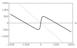
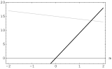
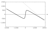
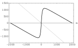
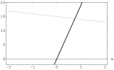
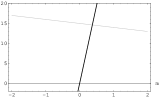
Figure 4: Plots of the left-hand side (in gray) and right-hand side (in black) of equation Eq. (25). Define $\alpha\equiv\frac{g}{2\pi^{2}}$. For each plot the parameters are: (a) $\Lambda=100$, $m_{0}=0$, $\alpha=0.001$. (b) $\Lambda=100$, $m_{0}=15$, $\alpha=0.001$. (c) $\Lambda=100$, $m_{0}=1200$, $\alpha=0.001$. (d) $\Lambda=100$, $m_{0}=0$, $\alpha=0.002$. (e) $\Lambda=100$, $m_{0}=15$, $\alpha=0.002$. (f) $\Lambda=200$, $m_{0}=15$, $\alpha=0.001$.

As before, we use the Schwinger-Dyson equation Eq. (8), and after summing up the right-hand side as a geometric series, we arrive at the self-consistency condition for our ansatz Eq. (15):

$$m_{0}-m-f\gamma^{0} = -\Sigma(0)$$ (22)

$$= \frac{g}{2\pi^{2}}\left[-(f^{2}-m^{2})^{3/2}\,\gamma^{0}\right.$$

$$+m^{3}\log{\left(\frac{f+\sqrt{f^{2}-m^{2}}}{\Lambda+\sqrt{\Lambda^{2}+m^{2}}}\right)}$$

$$+m\Lambda\sqrt{\Lambda^{2}+m^{2}}$$

$$-mf\sqrt{f^{2}-m^{2}}\left.\phantom{\frac{0}{1}}\right].$$

Clearly Eq. (22) will not admit a non-trivial solution $f\neq 0$ unless $g$ is positive, which agrees with our intuition that the theory must exhibit attraction between particles of the same fermion number. The self-consistent condition Eq. (22) may be separated into two simultaneous equations:

$$f=\frac{g}{2\pi^{2}}(f^{2}-m^{2})^{3/2}$$ (23)

and

$$m_{0}-m = \frac{gm}{2\pi^{2}}\left[m^{2}\log{\left(\frac{f+\sqrt{f^{2}-m^{2}}}{\Lambda+\sqrt{\Lambda^{2}+m^{2}}}\right)}\right.$$ (24)

$$+\left.\vphantom{\frac{0}{1}}\Lambda\sqrt{\Lambda^{2}+m^{2}}-f\sqrt{f^{2}-m^{2}}\right].$$

It is important to bear in mind that Eqs. (23) and (24) were written under the assumption that $f\geq m$. For $f<m$ the $f$ dependence of the self-energy in Eq. (18) disappears. The trivial, Lorentz invariant solution $f=0$ to the self-consistent equations will always be present for any $m$, as should be the case when spontaneous breaking of a symmetry is observed.

Equation (23) can be readily solved for $f$ as a function of $m$ (imposing the condition that $f$ be real and positive), and the resulting $f(m)$ can be substituted into Eq. (24) to yield

$$m_{0}-m = \frac{gm}{2\pi^{2}}\left[m^{2}\log{\left(\frac{f(m)+\sqrt{f^{2}(m)-m^{2}}}{\Lambda+\sqrt{\Lambda^{2}+m^{2}}}\right)}\right.$$ (25)

$$+\left.\vphantom{\frac{0}{1}}\Lambda\sqrt{\Lambda^{2}+m^{2}}-f(m)\sqrt{f^{2}(m)-m^{2}}\right].$$

Equation (25) cannot be solved algebraically, but we may study some of its properties graphically. In Fig. 4 we have plotted the left-hand side and the right-hand side of Eq. (25) for various values of the parameters $g$, $m_{0}$ and $\Lambda$. As plot (a) illustrates, $m_{0}=0$ implies $m=0$, i.e., we cannot dynamically generate both a chemical potential and a mass term. For $m=m_{0}=0$ we have

$$f=\pi\sqrt{2/g}.$$ (26)

Plot (b) in Fig. 4 shows a $0<m_{0}\ll\Lambda$ for which the corresponding $m$ will be significantly less than $m_{0}$. Plot (c) in the same figure illustrates that a very large $m_{0}$ is needed before $m>m_{0}$, but such solutions are not physically meaningful because $m_{0}$ itself is already well beyond the energy scale for which our effective theory is supposed to hold. By comparing plot (b) to plot (e) we may see the effect of increasing $g$ for a given $m_{0}$ and $\Lambda$. A comparison of plots (b) and (f) should illustrate the effect of increasing $\Lambda$ with the other parameters fixed.

The plots in Fig. 5 illustrate the progression, as the parameter $\Lambda$ is increased for fixed $\alpha$, from an unstable theory in which bare masses $m_{0}$ on the order of $\Lambda$ are mapped to $m>\Lambda$, to a theory that maps such bare masses to $m<\Lambda$. Such an analysis of Eq. (25) reveals that the condition for this mass stability is

$$0<\frac{2\pi^{2}}{g\Lambda^{2}}<1$$ (27)

which is reminiscent of the condition Eq. (11) for chiral symmetry breaking in the NJL model (except that now the interaction has the opposite sign). Combining Eq. (27) with Eq. (26) (which was exact for $m_{0}$ but may serve approximately for $m_{0}$ small) we arrive at the requirement

$$0<f^{2}<\Lambda^{2}$$ (28)

which would surely have to hold if our theory were stable. Indeed, we may interpret Eq. (28) as saying that if we pick physically good parameters $g$, $m_{0}$ and $\Lambda$, we will have a stable theory with finite chemical potential $f$. The parameters for plots (a), (b), (d), (e), and (f) in Fig. 4 all give examples of such stable theories. As in NJL, the good parameters involve $g^{-1/2}$ large with respect to $\Lambda$, suggesting that Eq. (17) should be a low-energy approximation to a non-perturbative interaction of a full renormalizable theory that allows attraction between particles of the same fermion number sign.

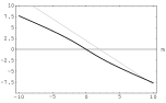
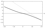
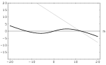
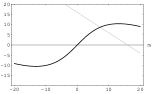
Figure 5: Plots of the left-hand side (in gray) and right-hand side (in black) of equation Eq. (25). For all of them $\alpha\equiv\frac{g}{2\pi^{2}}=0.01$. (a) $\Lambda=m_{0}=2$. (b) $\Lambda=m_{0}=8$. (c) $\Lambda=m_{0}=12$. (d) $\Lambda=m_{0}=16$.

The issue of how the form of the self-consistent equations will depend on the choice of regulator for the integral in Eq. (18) is not an entirely straightforward matter. But it seems to be a solid conclusion that, for positive fermion self-coupling $g$, the solutions to such self-consistent equations show the presence of LI-breaking vacua. In the next section of this paper we offer an alternative approach that strengthens this conclusion and that sheds further light on the issue of stability.

V Consequences for Emergent Photons

The theory

$$\mathcal{L}=\bar{\psi}(i\partial\!\!\!/-m_{0})\psi+\frac{g}{2}(\bar{\psi}\gamma^{\mu}\psi)^{2}$$ (29)

is equivalent to

$$\mathcal{L}^{\prime}=\bar{\psi}(i\partial\!\!\!/-A\!\!\!/-m_{0})\psi-\frac{A^{2}}{2g}.$$ (30)

Since we argued that Eq. (29) may spontaneously break LI by giving a finite $\langle\bar{\psi}\gamma^{\mu}\psi\rangle$, we conclude that $A^{\mu}$ in Eq. (30) would also have a finite VEV, since, by the algebraic equation of motion,

$$A^{\mu}=-g\bar{\psi}\gamma^{\mu}\psi.$$ (31)

This interpretation agrees with the observation that Eq. (30) has a vector boson field whose mass term carries the wrong sign if $g>0$, indicating that the zero-field state is not a good vacuum. To find the correct vacuum for the theory we must carry out the path integral over the fermion field to obtain the effective action $\Gamma[A]$, and then minimize that quantity. The field $A^{\mu}$ is minimally coupled to $\psi$, so that the computation should proceed as in QED. By the Ward identity we do not expect a correction to the mass term for $A^{\mu}$, as long as an adequate regulator is used. But we do expect to get terms in the effective action that go as $A^{4}$ and higher even powers of the auxiliary field.

Since we have reason to believe that QED is stable for any value of the charge $e$, it therefore seems logical to expect that the effective action for $A^{\mu}$ in Eq. (30) gives it a finite time-like VEV, which would imply a finite VEV for $\bar{\psi}\gamma^{\mu}\psi$ in the theory of Eq. (29). We argued in the previous section that $g$ must be large for the theory described by Eq. (29) to be stable. This too seems natural in light of Eq. (30), because a large $g$ makes the $A^{2}$ term small, so that the instability created by it may be easily controlled by the interaction with the fermions, yielding a VEV for $A^{\mu}$ that lies within the energy range of the effective theory.

Armed with Eq. (30) it would seem possible to carry out the program proposed by Bjorken, and by Kraus and Tomboulis, in order to arrive at an approximation of QED in which the photons are composite Goldstone bosons. It is conceivable that a complicated theory of self-interacting fermions, perhaps one with non-standard kinetic terms, might similarly yield a VEV for $\bar{\psi}\frac{i}{2}(\gamma_{\mu}\buildrel\rightarrow\over{\partial}_{\nu}-\gamma_{\mu}\buildrel\leftarrow\over{\partial}_{\nu})\psi$, allowing the project of dynamically generating linearized gravity to go forward. We leave this for future investigation.

VI Phenomenology of Lorentz Violation by a Background Source

A separate line of thought that might be pursued from this work concerns a phenomenology of Lorentz violation in electrodynamics with a background source. That is, we might imagine that the fermions of the universe have some interaction that plays the role of Eq. (17) in giving a VEV to $\bar{\psi}\gamma^{\mu}\psi$, and that in addition they have a $U(1)$ gauge coupling (at this stage we have abandoned the project of producing composite photons). Then the $U(1)$ gauge field may interact with a charged background and we would be breaking LI in electrodynamics by introducing a preferred frame: the rest frame of the background source.

The possibility of a vacuum that breaks LI and has non-trivial optical properties has already been investigated in AndrianovSoldati ; Soldati . This work, however, deals with significantly more complicated models, both in terms of the interactions that spontaneously break LI and of the optical properties of the resulting vacuum. To obtain a phenomenology for our own simpler proposal, we consider a free photon Lagrangian of the form

$$\mathcal{L}_{0}^{\mathrm{photon}}=-\frac{1}{4}F_{\mu\nu}^{2}-j_{\mu}A^{\mu}$$ (32)

where $j^{\mu}=e\langle\bar{\psi}\gamma^{\mu}\psi\rangle$, thought of as an external source. The corresponding propagator for the free photon is

$$\langle T\{A^{\mu}(x)A^{\nu}(y)\}\rangle=D^{\mu\nu}_{F}(x-y)+\langle A^{\mu}(x)\rangle_{j}\,\langle A^{\nu}(y)\rangle_{j}$$ (33)

where $D^{\mu\nu}(x-y)$ is the connected photon propagator and $\langle A^{\mu}(x)\rangle_{j}$ is the expectation value of $A^{\mu}$ in the presence of the external source.

If we take $j^{\mu}$ constant and naively attempt to calculate the classical expectation value of $A^{\mu}$ in the presence of a constant source by integrating the Green function for electrodynamics, we will get a volume divergence. We may attempt to regulate this volume divergence by introducing a photon mass $\mu$, which gives the result

$$\langle A^{\mu}(x)\rangle_{j}=\frac{j^{\mu}}{\mu^{2}}.$$ (34)

(It is trivial to check that this is a solution to $\partial^{2}A^{\mu}+\mu^{2}A^{\mu}=j^{\mu}$, the wave equation for the massive photon field with a source.) This is not satisfactory because the disconnected term in Eq. (33) will be proportional to $\mu^{-4}$ and Feynman diagrams computed with our modified photon propagator would produce results that depend strongly on what we took for a regulator. In fact the mass is physical and analogous to the effective photon mass first described by the London brothers in their theory of the electromagnetic behavior of superconductors London . (Using the language of particle physics we may say that, in the presence of a $U(1)$ gauge field, the VEV $\langle\bar{\psi}\gamma^{\mu}\psi\rangle$ spontaneously breaks the gauge invariance and gives a mass to the boson, as in the Higgs mechanism.)

Photons in a superconductor propagate through a constant electromagnetic source. In a simplified picture, we may think of it as a current density set up by the motion of charge carriers of mass $m$ and charge $e$, moving with a velocity $\vec{u}$. The proper charge density is $\rho_{0}$. The proper velocity of the charge carriers is $\eta^{\mu}=(1,\vec{u})/\sqrt{1-u^{2}}$. The source is then $j^{\mu}=\rho_{0}\eta^{\mu}=\rho_{0}p^{\mu}/m$, where $p^{\mu}$ is the classical energy momentum of the charge carriers. We may think of $m$ and $\rho_{0}$ as deriving from the solutions to the parameters in a self-consistent equation such as we had in Eq. (25).

The canonical energy momentum $P^{\mu}$ of the system is $P^{\mu}=m\eta^{\mu}+eA^{\mu}=mj^{\mu}/\rho_{0}+eA^{\mu}$. As is discussed in the superconductivity literature (see, for instance, Chap. 8 in Kittel ), the superconducting state has zero canonical energy momentum, which leads to the London equation

$$j^{\mu}=-\frac{e\rho_{0}}{m}A^{\mu}.$$ (35)

With this $j^{\mu}$ inserted into the right-hand side of $\partial^{2}A^{\mu}=j^{\mu}$ (the wave equation for the photon field in the Lorenz gauge), we find that we have a solution to the wave equation of a massive $A^{\mu}$ with no source and a mass $\mu^{2}=e\rho_{0}/m$:

$$\partial^{2}A^{\mu}+\frac{e\rho_{0}}{m}A^{\mu}=0.$$ (36)

If we solve for $A^{\mu}$ in Eq. (35) and substitute this back into Eq. (33), we get that

$$\langle T\{A^{\mu}(x)A^{\nu}(y)\}\rangle=D^{\mu\nu}_{F}(x-y)+\frac{m^{2}}{e^{2}j^{2}}j^{\mu}j^{\nu}.$$ (37)

Notice that if $j^{\mu}(x)$ is not constant, then Fourier transformation of the second term in Eq. (37) will not yield, in Feynman diagram vertices, the usual energy-momentum conserving delta function. Therefore, presumed small violations of energy or momentum conservation in electromagnetic processes could conceivably be parametrized by the space-time variation of the background source.

With Eq. (37) and a rule for external massive photon legs, one may then go ahead and calculate the amplitude for various electromagnetic processes with this modified photon propagator, and parametrize supposed observed violations of LI (see phenomenology1 ; phenomenology2 ; phenomenology3 ) by $j^{\mu}$. If we can make an estimate of the size of the the mass $m$ of the background charges, experimental limits on the photon mass ($<2\times 10^{-16}$ eV according to ReviewPP ) will provide a limit on the VEV of $\bar{\psi}\gamma^{\mu}\psi$, in light of Eq. (35).

VII Other Possible Consequences of This Mechanism

There are other consequences of a VEV $\langle\bar{\psi}\gamma^{\mu}\psi\rangle\neq 0$ on which we may speculate. Such a background may have cosmological effects, a line of thought which might connect, for instance, with Fried . Also, it is conceivable that such a VEV might have some relation to the problem of baryogenesis, since it gives the background finite fermion number and spontaneously breaks CPT, a violation which can ease the Sakharov condition of thermodynamical non-equilibrium baryogenesis .

It has recently been suggested that the standard model might be formulated without a Higgs scalar field, by introducing instead fermion self-interactions which do not destroy the renormalizability of the theory if there are nonzero UV fixed points under the renormalization group operation noHiggs . That work, published after the first manuscript of the present paper had appeared in the pre-print archive, might well relate to the mechanism we have described, particularly in light of what was discussed in the previous section of this paper.

All these tentative ideas are left for possible consideration in the future.

VIII Conclusions

We have presented a stable effective theory in which a chemical potential term is dynamically generated, thus spontaneously breaking LI (as well as C, CP, and CPT). The main reasons why this theory might be interesting are the following: (a) that it might serve as the starting point for models with emergent gauge bosons, (b) that it could conceivably point to LI breaking in other more natural theories that share its fundamental attribute: attraction between particles of the same fermion number sign (something that is seen in non-Abelian gauge theories such as QCD, which allows bound states with non-zero baryon number) and (c) that it produces something that could perhaps interest those who study the phenomenology of Lorentz violation in electrodynamics: the breaking of LI by introducing a background source with its own rest frame.

All of these remain somewhat problematic because (a) our work applies directly not to the more interesting case of generating emergent gravitons, but only to photons, (b) so far we have not been able to produce models that spontaneously break LI which are significantly more natural than Eq. (29), which is a non-renormalizable theory in which the fermion self-coupling has the opposite sign to what is obtained by integrating out a heavy $U(1)$ gauge boson, and (c) it remains to be seen whether a phenomenology of electrodynamics with a background source is of any interest to the effort of explaining the supposed indications of Lorentz violation in cosmic ray data and other measurements. These are all areas that would need to be explored in order to make more concrete and useful the ideas presented here.

- (1) V. A. Kostelecky and S. Samuel, Phys. Rev. D 39, 683 (1989); V. A. Kostelecky and R. Potting, Nucl. Phys. B359, 545 (1991).
- (2) J. Madore, gr-qc/9906059.
- (3) H. Ooguri and C. Vafa, Adv. Theor. Math. Phys. 7, 53 (2003) [hep-th/0302109].
- (4) S. R. Coleman and S. L. Glashow, Phys. Rev. D 59, 116008 (1999) [hep-ph/9812418]; Phys. Lett. B405, 249 (1997) [hep-ph/9703240].
- (5) J. Magueijo and L. Smolin, Phys. Rev. Lett. 88, 190403 (2002) [hep-th/0112090]; Phys. Rev. D 67, 044017 (2003) [gr-qc/0207085].
- (6) G. Amelino-Camelia, Nature (London) 418, 34 (2002) [gr-qc/0207049].
- (7) F. R. Klinkhamer, Nucl. Phys. B535, 233 (1998) [hep-th/9805095]; Nucl. Phys. B578, 277 (2000) [hep-th/9912169]; F. R. Klinkhamer and J. Nishimura, Phys. Rev. D 63, 097701 (2001) [hep-th/0006154]; F. R. Klinkhamer and C. Mayer, Nucl. Phys. B616, 215 (2001) [hep-th/0105310]; F. R. Klinkhamer and J. Schimmel, Nucl. Phys. B639, 241 (2002) [hep-th/0205038].
- (8) D. Colladay and V. A. Kostelecky, Phys. Rev. D 58, 116002 (1998) [hep-ph/9809521]; V. A. Kostelecky and R. Lehnert, Phys. Rev. D 63, 065008 (2001) [hep-th/0012060].
- (9) P. Kraus and E. T. Tomboulis, Phys. Rev. D 66, 045015 (2002) [hep-th/0203221].
- (10) J. D. Bjorken, Ann. Phys. (N. Y.) 24, 194 (1963).
- (11) Y. Nambu and G. Jona-Lasinio, Phys. Rev. 122, 345 (1961); 124, 246 (1961).
- (12) Y. Nambu, Phys. Rev. 117, 648 (1960).
- (13) M. G. Alford, K. Rajagopal and F. Wilczek, Nucl. Phys. A638, 515C (1998) [hep-ph/9802284].
- (14) M. G. Alford, J. A. Bowers, J. M. Cheyne and G. A. Cowan, Phys. Rev. D 67, 054018 (2003) [hep-ph/0210106].
- (15) C. Wetterich, Phys. Rev. D 64, 036003 (2001) [hep-ph/0008150]; J. Berges and C. Wetterich, Phys. Lett. B512, 85 (2001) [hep-ph/0012311].
- (16) G. ’t Hooft, Nucl. Phys. B33, 173 (1971); 35, 167 (1971).
- (17) L. O’Raifeartaigh and N. Straumann, Rev. Mod. Phys. 72, 1 (2000).
- (18) J. D. Jackson and L. B. Okun, Rev. Mod. Phys. 73, 663 (2001) [hep-ph/0012061].
- (19) J .D. Bjorken, hep-th/0111196.
- (20) S. Weinberg and E. Witten, Phys. Lett. B96, 59 (1980).
- (21) C. Armendariz-Picon, T. Damour and V. Mukhanov, Phys. Lett. B458, 209 (1999) [hep-th/9904075].
- (22) R. R. Caldwell, M. Kamionkowski and N. N. Weinberg, Phys. Rev. Lett. 91, 071301 (2003) [astro-ph/0302506].
- (23) N. Arkani-Hamed, H. C. Cheng, M. A. Luty and S. Mukohyama, hep-th/0312099; N. Arkani-Hamed, P. Creminelli, S. Mukohyama and M. Zaldarriaga, JCAP 0404, 001 (2004) [hep-th/0312100].
- (24) S. Weinberg, The Quantum Theory of Fields, Vol. 2, Cambridge (1996).
- (25) K. I. Aoki, K. Morikawa, J. I. Sumi, H. Terao and M. Tomoyose, Phys. Rev. D 61, 045008 (2000) [hep-th/9908043].
- (26) J. Bardeen, L. Cooper, and J. Schrieffer, Phys. Rev. 106, 162 (1957); Phys. Rev. 108 1175 (1957).
- (27) R. F. Streater and A. S. Wightman, PCT, Spin and Statistics, and All That, Benjamin, (1964).
- (28) F. J. Dyson, Phys. Rev. 85, 631 (1952).
- (29) A. A. Andrianov and R. Soldati, Phys. Rev. D 51, 5961 (1995); Phys. Lett. B435, 449 (1998) [hep-ph/9804448]; A. A. Andrianov, R. Soldati and L. Sorbo, Phys. Rev. D 59, 025002 (1999) [hep-th/9806220].
- (30) A. A. Andrianov, P. Giacconi and R. Soldati, JHEP 0202, 030 (2002) [hep-th/0110279].
- (31) F. London and H. London, Proc. Roy. Soc. A149 71 (1935).
- (32) C. Kittel, Quantum Theory of Solids, Wiley (1963).
- (33) V. A. Kostelecky, R. Lehnert and M. J. Perry, astro-ph/0212003.
- (34) S. M. Carroll, G. B. Field and R. Jackiw, Phys. Rev. D 41, 1231 (1990).
- (35) V. A. Kostelecky and M. Mewes, Phys. Rev. D 66, 056005 (2002) [hep-ph/0205211].
- (36) O. Bertolami and C. S. Carvalho, Phys. Rev. D 61, 103002 (2000) [gr-qc/9912117]; O. Bertolami, Gen. Rel. Grav. 34, 707 (2002) [astro-ph/0012462].
- (37) K. Hagiwara et al. [Particle Data Group Collaboration], Phys. Rev. D 66, 010001 (2002).
- (38) H. M. Fried, hep-th/0310095.
- (39) O. Bertolami, D. Colladay, V. A. Kostelecky and R. Potting, Phys. Lett. B395, 178 (1997) [hep-ph/9612437].
- (40) H. Gies, J. Jaeckel and C. Wetterich, Phys. Rev. D (to be published), hep-ph/0312034.