hep-th/0311125

Abstract

We determine solutions to 5D Einstein gravity with a discrete fifth dimension. The properties of the solutions depend on the discretization scheme we use and some of them have no continuum counterpart. In particular, we find that the neglect of the lapse field (along the discretized direction) gives rise to Randall-Sundrum type metric with a negative tension brane. However, no brane source is required. We show that this result is robust under changes in the discretization scheme. The inclusion of the lapse field gives rise to solutions whose continuum limit is gauge fixed by the discretization scheme. We find however one particular scheme which leads to an undetermined lapse reflecting the reparametrization invariance of the continuum theory. We also find other solutions, with no continuum counterpart with changes in the metric signature or avoidance of singularity. We show that the models allow a continuous mass spectrum for the gravitons with an effective 4D interaction at small scales. We also discuss some cosmological solutions.

1 Introduction

The possibility that space-time has more than four dimensions has been considered for many years. The Kaluza-Klein approach, widely used in superstring constructions and brane world models, relies on the assumption that each four dimensional space-time point is replaced by a compact internal manifold. Another possibility which was considered recently is to have an infinite fifth dimension with a negative cosmological constant, the four dimensional universe being confined to a 3-brane [1] on which gravity is localised. A generic feature of such models with continuous extra-dimensions is that the field excitations in the internal manifold are seen by four dimensional observers as a tower of infinitely many massive particles. This holds in particular for excitations of the metric with non zero momentum in the internal dimensions, resulting in a tower of massive gravitons. On the other hand, theories with a single (or a finite number of) massive graviton have also been considered. In particular it is well known, that there is only one ghost-free quadratic action for a massive spin 2 field, first introduced by Pauli and Fierz [2]. Going beyond quadratic order, one is lead to theories with several coupled metrics [3, 4]. Such theories, which we will call generically here multigravity, have been investigated in the past in relation to strong interaction [3], and more recently by various authors [5, 6] in particular in relation with discrete extra-dimensions [7, 6]. Discrete extra dimensions have also been considered in the spirit of non-commutative geometry [8].

Theories with massive graviton excitations are likely to suffer in general from several pathologies which could prevent them from being very useful to describe the real world. It includes the celebrated van Dam-Veltman-Zakharov (vDVZ) discontinuity [9], as well as the propagation of ghost-like fields when one considers an action which goes beyond quadratic orders [4]. Nonetheless some of these theories have promising phenomenological properties, in particular in relation with cosmology [11], and some of the drawbacks mentioned above seem to be curable [12]. In the perspective of better understanding theories with multiple gravitons, it is interesting to contrast theories obtained from a parent theory which is known to be fully consistent, with the parent theory itself. This has been done in the past using Kaluza-Klein compactification [13]. Here we follow a similar path by comparing simple solutions of theories obtained by discretizing one dimension in five dimensional (5D) general relativity to solution of the continuum theory. Namely we consider the extra dimension to be given by a one dimensional lattice, to each point of the lattice is associated a four dimensional space-time with a metric. We determine the coupling of the metrics by the requirement that the continuum limit should be given by five-dimensional gravity. The discrete action should respect as much as possible the symmetries of the 5D action, otherwise new degrees of freedom appear which are in general ghost-like. The actions we shall consider break explicitly the reparametrization invariance along the fifth direction. Although at the linear level the theory is free from ghosts, they may appear at the non linear level [4].

The paper is organized as follows. In Section 2, we rewrite in a way convenient for discretization the 5D Einstein-Hilbert action and accordingly recall different ways to parametrize 5D AdS space-time as sliced by 4D Minkowski space-time. We then (Section 3) turn to a first naive discretization scheme, where the lapse and shift fields (see below) are omitted. We show in particular that this allows one to get a brane world bulk solution with no source brane included. However, this solution corresponds to a negative tension brane. We show next how one can also recover the positive tension configuration, at the price of introducing a fine-tuned brane source in the discretized theory. Then we turn to include the lapse in our discretization scheme, and discuss issues related to reparametrization invariance along the discretized dimension. In Section 4 we calculate, in the model without lapse field, the static gravitational potential between two pointlike particles and show that it is 4D at small length scales and becomes 5D at large distances. We then comment on the vDVZ discontinuity in this model. In section 5 we discuss cosmological solutions of the discretized theory. Our conclusions are collected in Section 6.

2 Continuum theory: Five dimensional General Relativity

For the purpose of discretizing a space-like dimension, parametrized by coordinate $y$, it is convenient to rewrite the 5D Einstein-Hilbert action

$$S_{EH}=M_{(5)}^{3}\int d^{5}X\sqrt{-\tilde{g}}(\tilde{R}-2\tilde{\Lambda}),$$ (1)

using a 4+1 splitting of space time. Above, and in the following, we use expressions with a tilde for quantities of the 5D continuum theory, like the 5D metric $\tilde{g}_{AB}$, and upper case Latin letters from the beginning of the alphabet, $A,B,C...$ to denote 5D indices, $\tilde{\Lambda}$ is the 5D cosmological constant and $M_{(5)}$ is the 5D reduced Planck mass. After an integration by parts, (1) is rephrased into

$$M_{(5)}^{3}\int d^{4}xdy\sqrt{-g}{\cal N}\left\{R-2\tilde{\Lambda}+K_{\mu\nu}K_{\alpha\beta}\left(g^{\mu\nu}g^{\alpha\beta}-g^{\mu\alpha}g^{\nu\beta}\right)\right\},$$ (2)

where $K_{\mu\nu}$ is the extrinsic curvature of surfaces ${\cal H}_{y}$ located at constant $y$, and we have introduced in a standard way the lapse ${\cal N}$, the shift $N_{\mu}$, and induced metric $g_{\mu\nu}$ on ${\cal H}_{y}$ whose Ricci scalar is denoted by $R$. Note that here and in the following, lower case Greek letters, $\mu,\nu,\alpha,...$ will be denoting 4D indices, i.e. indices parallel to ${\cal H}_{y}$. The extrinsic curvature is defined by

$$K_{\mu\nu}=\frac{1}{2{\cal N}}\left(g^{\prime}_{\mu\nu}-D_{\mu}N_{\nu}-D_{\nu}N_{\mu}\right),$$ (3)

where $D_{\mu}$ is the covariant derivative associated with the induced metric $g_{\mu\nu}$ and a prime denotes an ordinary derivative with respect to $y$. The fields ${\cal N}$, ${N}_{\mu}$ and $g_{\mu\nu}$ are simply related to the components of the 5D metric $\tilde{g}_{AB}$ by

$$\tilde{g}_{\mu\nu} = g_{\mu\nu},$$ (4)

$$\tilde{g}_{\mu y} = N_{\mu}\equiv g_{\mu\alpha}N^{\alpha},$$ (5)

$$\tilde{g}_{yy} = {\cal N}^{2}+g_{\mu\nu}N^{\mu}N^{\nu}.$$ (6)

The equations of motions derived from the action (2) varying with respect to ${\cal N}$, $N^{\mu}$ and $g^{\mu\nu}$ yield respectively

$$R-2\tilde{\Lambda} = K^{2}-K^{\rho}_{\sigma}K^{\sigma}_{\rho}$$ (7)

$$0 = D^{\mu}K-D^{\nu}K^{\mu}_{\nu}$$ (8)

$$G_{\mu\nu}+\tilde{\Lambda}g_{\mu\nu} = \frac{1}{2}g_{\mu\nu}\left(K^{2}-K^{\rho}_{\sigma}K^{\sigma}_{\rho}\right)+\frac{D_{\mu}D_{\nu}{\cal N}-g_{\mu\nu}D^{\rho}D_{\rho}{\cal N}}{\cal N}-g_{\rho\mu}g_{\sigma\nu}\frac{\partial_{y}\left\{\sqrt{-g}\left(Kg^{\rho\sigma}-K^{\rho\sigma}\right)\right\}}{{\cal N}\sqrt{-g}}$$ (9)

$$-\frac{2}{N}\left\{D_{\nu}\left(N_{\mu}K\right)-D_{\rho}\left(K^{\rho}_{\nu}N_{\mu}\right)-\frac{1}{2}g_{\mu\nu}D^{\rho}\left(KN_{\rho}\right)+\frac{1}{2}D^{\rho}\left(N_{\rho}K_{\mu\nu}\right)\right\}$$

$$+2\left(K^{\rho}_{\mu}K_{\rho\nu}-KK_{\mu\nu}\right),$$

where $G_{\mu\nu}$ is the Einstein tensor for four dimensional metric $g_{\mu\nu}$, and $K$ is defined by $K\equiv K_{\mu\nu}g^{\mu\nu}$. When $N_{\mu}$ vanishes, equations (7) and (9) reduce respectively to

$$R-2\tilde{\Lambda} = {1\over 4{\cal N}^{2}}g^{\prime}_{\mu\nu}g^{\prime}_{\alpha\beta}(g^{\mu\nu}g^{\alpha\beta}-g^{\mu\alpha}g^{\nu\beta}),$$ (10)

$$G_{\mu\nu}+\tilde{\Lambda}g_{\mu\nu} = {1\over{\cal N}}\left(D_{\mu}D_{\nu}{\cal N}-g_{\mu\nu}\ g^{\rho\sigma}D_{\rho}D_{\sigma}{\cal N}\right)$$ (11)

$$+ {g_{\mu\nu}\over{\cal N}^{2}}\left(-{1\over 8}(g^{\prime}_{\alpha\beta}g^{\alpha\beta})^{2}+{3\over 8}g^{\prime}_{\alpha\beta}g^{\prime}_{\lambda\delta}g^{\delta\beta}g^{\lambda\alpha}-{1\over 2}g"_{\alpha\beta}g^{\alpha\beta}+{1\over 2}{{\cal N}^{\prime}\over{\cal N}}g^{\prime}_{\alpha\beta}g^{\alpha\beta}\right)$$

$$+ {1\over 4{\cal N}^{2}}g^{\prime}_{\mu\nu}(g^{\prime}_{\alpha\beta}g^{\alpha\beta})+{1\over 2{\cal N}^{2}}g"_{\mu\nu}-{{\cal N}^{\prime}\over 2{\cal N}^{3}}g^{\prime}_{\mu\nu}-{1\over 2{\cal N}^{2}}g^{\prime}_{\mu\alpha}g^{\prime}_{\nu\beta}g^{\alpha\beta},$$

where $G_{\mu\nu}$ is the Einstein tensor of the 4D metric $g_{\mu\nu}$. We then consider simple solutions of the 5D Einstein equations, which are slicings of the 5D space-time by 4D Minkowski space-time. We write accordingly ${\cal N}={\cal N}(y)$, $g_{\mu\nu}(x^{\alpha},y)=\Omega(y)\eta_{\mu\nu}$, where $\eta_{\mu\nu}$ is a 4D Minkoswski metric, and we keep $N_{\mu}=0$. Then equations (8) are identically satisfied and the equations (11) and (10) reduce to

$$\frac{1}{{\cal N}}\left(\frac{\Omega^{\prime}}{{\cal N}}\right)^{\prime} = -\frac{2}{3}\tilde{\Lambda}\Omega,$$ (12)

$$\left({\Omega^{\prime}\over\ {\cal N}}\right)^{2} = -{2\over 3}\tilde{\Lambda}\Omega^{2}.$$ (13)

One notes that the above equations are not independent, the first being a consequence of the second. This is of course a simple consequence of the $y$ reparametrization invariance of the 5D Einstein-Hilbert action (1) and tells us that we cannot solve both for ${\cal N}$ and $\Omega$ out of the equations of motion. Indeed by choosing a Gaussian Normal gauge, defined here simply by setting ${\cal N}$ to 1, one can get the following solution for the 5D line element

$$ds^{2} \equiv \tilde{g}_{AB}^{(1)}dX^{A}dX^{B}$$ (14)

$$= dy^{2}+\exp\left(\epsilon y\sqrt{-\frac{2}{3}\tilde{\Lambda}}\right)dx^{\mu}dx^{\nu}\eta_{\mu\nu},$$

where we have assumed $\tilde{\Lambda}$ to be negative. These solutions are well known parametrization of a Poincaré patch of $AdS_{5}$. If one instead puts an absolute value on $y$, in the above line element, and considers then the metric $\tilde{g}_{AB}^{(2)}$ given by

$$ds^{2} \equiv \tilde{g}_{AB}^{(2)}dX^{A}dX^{B}$$ (15)

$$= dy^{2}+\exp\left(\epsilon|y|\sqrt{-\frac{2}{3}\tilde{\Lambda}}\right)dx^{\mu}dx^{\nu}\eta_{\mu\nu},$$

one obtains the well known Randall-Sundrum [1] type of metric which are simply given by gluing two identical patches of the space-time parametrized by metric $\tilde{g}_{AB}^{(1)}$ along a brane of positive ($\epsilon=-1$) or negative ($\epsilon=+1$) tension. This requires a fine tuning between the brane tension $\tilde{\sigma}$ and the bulk (negative) cosmological constant $\tilde{\Lambda}$ given by

$$\tilde{\sigma}^{2}=-6M_{(5)}^{6}\tilde{\Lambda},$$ (16)

where normalization of the brane tension is set by its action,

$$-\int d^{4}xdy\sqrt{-g}2\delta(y)\epsilon\tilde{\sigma},$$ (17)

that was added to the Einstein-Hilbert action (2) to get (15). Another parametrization $\tilde{g}^{(3)}_{AB}$ of the space time described by the line element (14) that we will use in the following, is given by

$$ds^{2} \equiv \tilde{g}^{(3)}_{AB}dX^{A}dX^{B}$$ (18)

$$= -\frac{3}{2\tilde{\Lambda}}\frac{dz^{2}}{(z+\tilde{z}_{0})^{2}}+Z_{0}(z+\tilde{z}_{0})\eta_{\mu\nu}dx^{\mu}dx^{\nu},$$ (19)

where $\tilde{z}_{0}$ and $Z_{0}$ are some constants, and $z$ is related to $y$ of equation (14) by $Z_{0}(z+\tilde{z}_{0})=\exp\left(\epsilon y\sqrt{-2/3\tilde{\Lambda}}\right)$.

3 Theories with a discretized extra dimension

We are now turning to the type of theories which will be of interest in this work. Those can be obtained from the Einstein-Hilbert action (2) where one discretizes the continuuous coordinate $y$ with a spacing $a$ between two adjacent sites (labelled by an index $i$). It was shown in reference [14] how to obtain such a discretization, maintaining $y$ dependant 4D gauge invariance on each sites. This can be done by the mean of link fields $X^{\mu}(i,i+1;x)$ [6], mapping between site $i$ and site $i+1$, which were explicitly build out of the $5D$ metric in reference [14]. One can proceed as follows, we first note that the $y$ derivatives arising in action (2) only appear in the extrinsic curvature $K_{\mu\nu}$ (as defined in Eq. (3)). The latter can be expressed in term of the Lie derivative ${\cal L}_{D_{y}}$ along the vector field $D_{y}$ defined by $D_{y}=\partial_{y}-N^{\mu}\partial_{\mu}$, such that

$$K_{\mu\nu}=\frac{1}{2{\cal N}}{\cal L}_{D_{y}}g_{\mu\nu}.$$ (20)

To discretize action (2) in a way which conserve reparametrization invariances on each sites, we then simply replace every Lie derivative ${\cal L}_{D_{y}}$, acting on a tensor $T(x^{\mu},y)$, by its discrete counterpart $\Delta_{\cal L}$ defined as

$$\Delta_{\cal L}T_{i}={W(i,i+1)T_{i+1}-T_{i}\over a},$$ (21)

where the action of the transport operator $W(i,i+1)$ on the components of tensor $T$ is given by

$$\left[W(i,i+1)T_{i+1}\right]_{\mu_{1},\dots\mu_{r}}(x)=\partial_{\mu_{1}}X^{\nu_{1}}\dots\partial_{\mu_{r}}X^{\nu_{r}}T_{i+1}\left(X^{\mu}(i,i+1;x)\right)_{\nu_{1},\dots\nu_{r}}.$$ (22)

The transport operators $W(i,i+1)$ are generated by the shift vector fields [14] and at leading order in the transverse lattice spacing $a$, $X^{\mu}$ is given by

$$X^{\mu}(i,i+1,x)=x^{\mu}+aN^{\mu}(y_{i},x)+{\cal O}(a^{2}),$$ (23)

where $y_{i}$ is the $y$ coordinate of site $i$. If one then makes a gauge choice such that $X^{\mu}(i,i+1,x)=x^{\mu}$, one is lead to consider theories of a set of 4D metrics $g^{i}_{\mu\nu}$, and 4D scalar lapse field ${\cal N}_{i}$ with actions of the form

$$S[g_{i},{\cal N}_{i}]=\Sigma_{i}M_{(4)}^{2}\int d^{4}x\sqrt{-g_{i}}{\cal N}_{i}\left(R(g_{i})-2\Lambda\right)-\int d^{4}x\frac{M_{(4)}^{2}}{{\cal N}_{i}}V(g_{i},g_{i+1}),$$ (24)

where $V(g_{i},g_{i+1})$ is an interaction term between the metrics $g^{i}_{\mu\nu}$ and $g^{i+1}_{\mu\nu}$, and $M_{(4)}$ is a mass scale which sets the coupling scale between the metric on a given site and matter sources that one may wish to put on the same site. If one insists in keeping the link with the 5D theory, one should verify the equation of motion for $X^{\sigma}$. The latter read (in the gauge $X^{\mu}=x^{\mu}$)

$$0 = \frac{2{\cal N}_{i}}{\sqrt{-g_{i}}}\partial_{\mu}\left(\frac{\sqrt{-g_{i}}}{{\cal N}_{i}}g_{\sigma\nu}^{i+1}\left(g_{\alpha\beta}^{i+1}-g_{\alpha\beta}^{i}\right)\left(g^{\mu\nu}_{i}g_{i}^{\alpha\beta}-g^{\mu\alpha}_{i}g^{\nu\beta}_{i}\right)\right)$$ (25)

$$-\left(\partial_{\sigma}g_{\mu\nu}^{i+1}\right)\left(g_{\alpha\beta}^{i+1}-g_{\alpha\beta}^{i}\right)\left(g^{\mu\nu}_{i}g_{i}^{\alpha\beta}-g^{\mu\alpha}_{i}g^{\nu\beta}_{i}\right)$$

and reduce to equation (8) in the continuum limit. This equation is somehow similar to a Kaluza-Klein consistency condition [15, 16]. Note that the index $i$ can be envisioned as labelling theory space sites in the spirit of the deconstruction program of Ref. [6], but theories under investigation here can also be considered without an explicit reference to a continuum limit, simply as theories of multigravity [3, 5]. In the latter case, one does not have to consider equation (25). We will, for most of the cases discussed in this paper, not include any matter fields so that each of the sites $i$ will only be considered endowed with a cosmological constant $\Lambda$ and will consider various possible interaction terms given by

$$V_{1}(g_{i},g_{i+1}) = -\frac{m^{2}}{4}\sqrt{-g_{i}}\left(g_{\mu\nu}^{i+1}-g_{\mu\nu}^{i}\right)\left(g_{\alpha\beta}^{i+1}-g_{\alpha\beta}^{i}\right)\left(g_{i}^{\mu\nu}g_{i}^{\alpha\beta}-g_{i}^{\mu\alpha}g_{i}^{\nu\beta}\right),$$ (26)

$$V_{2}(g_{i},g_{i+1}) = -\frac{m^{2}}{4}\sqrt{-g_{i}}\left(g^{\mu\nu}_{i+1}-g^{\mu\nu}_{i}\right)\left(g^{\alpha\beta}_{i+1}-g^{\alpha\beta}_{i}\right)\left(g^{i}_{\mu\nu}g^{i}_{\alpha\beta}-g^{i}_{\mu\alpha}g^{i}_{\nu\beta}\right),$$ (27)

$$V_{3}(g_{i},g_{i+1}) = \frac{m^{2}}{4}\sqrt{-g_{i}}\left(g^{\mu\nu}_{i+1}-g^{\mu\nu}_{i}\right)\left(g_{\alpha\beta}^{i+1}-g_{\alpha\beta}^{i}\right)\left(g^{i}_{\mu\nu}g_{i}^{\alpha\beta}-\delta^{\mu}_{\alpha}\delta^{\nu}_{\beta}\right),$$ (28)

where $g_{i}^{\mu\nu}$ is the inverse metric of $g_{\mu\nu}^{i}$. With such choices of interaction terms, action (24) is a simple minded discretization of the 5D pure gravity Einstein-Hilbert action (1), where one has set $N_{\mu}$ to zero. This can be seen explicitly using the following identification

$$m^{2} = \frac{1}{a^{2}},$$ (29)

$$M_{(4)}^{2} = M_{(5)}^{3}a,$$ (30)

$$\Lambda = \tilde{\Lambda},$$ (31)

$$g_{\mu\nu}^{i}(x^{\mu}) = \tilde{g}_{\mu\nu}(x^{\mu},y_{i}),$$ (32)

$${\cal N}_{i}(x^{\mu}) = {\cal N}(x^{\mu},y_{i}),$$ (33)

where $a$ is the size of the discretization step along $y$, and $y_{i}=ia$. Note that each of the three potential (26), (27) and (28) corresponds to a different way to implement the discretization procedure outlined in the beginning of this section, depending on whether one discretizes $K_{\mu\nu}={\cal L}_{D_{y}}g_{\mu\nu}/2{\cal N}$ or $K^{\mu\nu}=-{\cal L}_{D_{y}}g^{\mu\nu}/2{\cal N}$.

3.1 No lapse field and brane space-time with no brane source

We first set from the beginning the lapse fields ${\cal N}_{i}$ to one in the multigravity action $S[g_{i},{\cal N}_{i}]$ and consider solutions to the equations of motion derived from the simplified action for the metrics $g^{i}_{\mu\nu}$, $S[g_{i},1]$. We wish here to compare these solutions with solutions of the continuum theory defined by action (2) and seek solutions of the form

$$g_{\mu\nu}^{i}=\Omega^{i}\eta_{\mu\nu},$$ (34)

with $\Omega^{i}$ constants. Let us first consider the case of the interaction term $V_{1}$. After a straightforward calculation, the equation of motion for the metric $g_{i}$ reduces to

$$-\lambda=-2+f_{i}+\left(f_{i-1}\right)^{-1},$$ (35)

with $\lambda={2\Lambda/3m^{2}}$, and $f_{i}=\Omega_{i+1}/\Omega_{i}$. Equation (35) defines a sequence (see figure 1) which has two fixed points (for $\lambda$ obeying $\lambda(-1+\lambda/4)>0)$ $f_{+}$ and $f_{-}$ given by

$$f_{\pm}=\left(1-{\lambda\over 2}\right)\pm\sqrt{\lambda\left({\lambda\over 4}-1\right)}.$$ (36)

These two fixed points are each located on a different side from 1 (for negative $\lambda$) , which is the double root of the fixed point equation for $\lambda=0$. Let us first consider the solutions ${\cal F}_{\pm}$ defined by $\forall i,f_{i}=f_{\pm}$. This translates into

$$\Omega^{j}_{\pm}=\Omega^{0}_{\pm}\left(f_{\pm}\right)^{y_{j}/a}.$$ (37)

We then look at the limit of this solution when the discretization step $a$ goes to zero. ¿From equations (29) and (31), one has $\lambda=\frac{2}{3}\tilde{\Lambda}a^{2},$ which gives in the limit of small $a$

$$f_{\pm}\sim 1\pm\sqrt{-\lambda}\sim 1\pm\sqrt{-\frac{2}{3}\tilde{\Lambda}}a,,$$ (38)

leading to,

$$g_{\mu\nu}^{j}\sim\Omega^{0}_{\pm}\exp\left(\pm\sqrt{-\frac{2}{3}\tilde{\Lambda}}y_{j}\right)\eta_{\mu\nu}.$$ (39)

This matches the metric (14), and the fixed point solutions ${\cal F}_{\pm}$, in the limit of small $a$ thus each corresponds to a discretized version of a Poincaré patch of $AdS_{5}$.

However equation (35) has more interesting solutions, it can indeed be exactly solved to yield

$$\Omega^{j}=\left((f_{+})^{j}+{\cal K}(f_{-})^{j}\right)\frac{\Omega^{0}}{1+{\cal K}},$$ (40)

where ${\cal K}$ is an integration constant, related to $f_{0}$ by

$${\cal K}=-\frac{f_{+}-f_{0}}{f_{-}-f_{0}}.$$ (41)

Let us consider the case where ${\cal K}$ is positive, this is true if we choose $f_{0}$ to lie in between $f_{-}$ and $f_{+}$. Note first that, for a fixed value of $a$ different from zero, one can choose any positive value of ${\cal K}$. One easily finds that the limiting behaviour of the metric on site $i$, when $a$ is send to zero is given by

$$g_{\mu\nu}^{i}\sim\frac{2\Omega^{0}\sqrt{\cal K}}{(1+{\cal K})}{\rm cosh}\left(\sqrt{-\frac{2}{3}\Lambda}(y_{i}-\Upsilon)\right)\eta_{\mu\nu},$$ (42)

where $\Upsilon$ is a constant given by

$$\Upsilon=\sqrt{-{3\over 8\Lambda}}{\rm ln}({\cal K}).$$ (43)

It turns out that the solution (42) has exactly the same asymptotics as $y_{i}$ goes to $\pm\infty$ as the Randall-Sundrum metric (15) with a negative tension brane placed at $y=\Upsilon$. This is a quite remarkable feature since no brane has been considered. In particular no fine tuning of the form (16) is necessary.

One might be concerned about knowing to what extent this result depends on the form of the discretization scheme. We now investigate this question by searching for solutions of the form (34) with $V$ taken of the form

$$V={\cal C}_{1}V_{1}+{\cal C}_{2}V_{2}+{\cal C}_{3}V_{3},$$ (44)

by changing $m^{2}$ we can always assume that ${\cal C}_{1}+{\cal C}_{2}+{\cal C}_{3}=1$. This choice also insures that the multigravity action $S[g_{i},1]$ has the action (2) for a limit when $a$ goes to zero, with the same identification as in equations (29-33). It is then straightforward to work out the equations of motion for the metrics $g_{\mu\nu}^{i}$ and get for the ansatz (34) the following expression replacing equation (35)

$$-\lambda=G_{1}(f_{i})+G_{2}(f_{i-1}),$$ (45)

with

$$G_{1}(u) = -4{\cal C}_{1}-3{\cal C}_{2}+2+u\left(-\frac{1}{2}+\frac{3}{2}{\cal C}_{1}+\frac{1}{2}{\cal C}_{2}\right)$$ (46)

$$+\frac{1}{u}\left(-\frac{3}{2}+\frac{3}{2}{\cal C}_{1}+\frac{9}{2}{\cal C}_{2}\right)-\frac{2}{u^{2}}{\cal C}_{2},$$

$$G_{2}(u) = \frac{1}{u}\left(-\frac{1}{2}+\frac{3}{2}{\cal C}_{1}+\frac{1}{2}{\cal C}_{2}\right)+\frac{1}{u^{3}}\left(\frac{1}{2}-\frac{1}{2}{\cal C}_{1}-\frac{3}{2}{\cal C}_{2}\right)+\frac{{\cal C}_{2}}{u^{4}}.$$ (47)

It is easy to see that $u=1$ is still a double root to the equation $G_{1}(u)+G_{2}(u)=0$. For $\lambda<0$, this double root degenerates into two root $f_{\pm}$, which are given (for small enough $\lambda$) by

$$f_{\pm}-1\equiv\delta_{\pm}\sim\pm\sqrt{-\lambda}.$$ (48)

Notice that the above expression is independent of ${\cal C}_{1}$ and ${\cal C}_{2}$, as could have been expected, and matches the one found in equation (38). While in the vicinity of these roots the sequence $\delta_{i}$ defined by $f_{i}=1+\delta_{i}$ verifies

$$\delta_{i}=\delta_{i-1}+\delta_{\pm}^{2}-\delta_{i-1}^{2}.$$ (49)

This leads to the same kind of solution as above: namely a solution with the same asymptotics as the Randall-Sundrum solution with a negative tension brane.

There is an easy way to understand these solutions by comparing the equations of motion of the continuum theory (12-13) to the ones of the multigravity theory (35) (or (45)). Indeed, in the limit where $a$ goes to zero, equation (35) (or (45)) reduces to equation (12). If one then looks for solutions of (12), with ${\cal N}$ set to one, one finds that the most general solution is given by a linear combination of $\exp\left(ky\right)$ and $\exp(-ky)$ with $k$ given by $\sqrt{-2\Lambda/3}$. This matches what is found in the discretized theory. However, in the continuum theory, the equation of motion for ${\cal N}$, namely equation (13), allows to keep the decreasing or increasing exponential, but not a combination of the two. This also enables to understand that we did not find the solution with a positive tension brane (which would have been very interesting in many respects). Indeed, a linear combination of exponentials $\exp\pm ky$ (with positive coefficients) is an increasing function for large positive $y$ and a decreasing function for large negative $y$. So that the asymptotic jump of the first $y$-derivative of the 4D metric across the brane, defined as $[\Omega^{\prime}(+\infty)-\Omega^{\prime}(-\infty)]/[\Omega(+\infty)+\Omega(-\infty)]$, is necessarily positive. This is turn means that the brane tension has to be negative, as can be seen from the junction conditions. In the next subsection, we show how to recover the positive tension brane solution, introducing a brane source with fine-tuned tension. We then, in the last subsection, turn to investigate the discretized theory where the lapse field ${\cal N}$ is kept, which seems to be required if one wants to approach closer solutions to the continuum theory. Let us underline here, however, that the solution (40) is a perfectly honest solution of the multigravity theory defined by action $S[g_{i},1]$. To complete this discussion, let us add that the solution (40), and more generally solution of equation (45), can also differ much more dramatically from solutions of the 5D continuum theory. In particular, the fixed points solutions ${\cal F}_{\pm}$ are very tuned solutions. Indeed any departure of $f_{0}$, say as an “initial” choice , from $f_{\pm}$ leads either to the negative brane-like solution, or to other type of solution where the signature of the 4D metric can change (as can be seen from equation (40) with ${\cal K}<0$).

3.2 Positive tension brane and fine tuning

In this subsection (and only here), we include a brane source, located at fixed $y$, in the discretized theory considered above. We wish to recover the discretized Randall-Sundrum metric with a positive tension brane, and discuss how the fine tuning condition (16) is translated in the discretized theory. To do so, we simply add to the action $S[g_{i},1]$, considered above with the potential $V_{1}$, the discretized version of the action (17) which can be simply taken to be

$$-\int d^{4}x\sqrt{-g_{0}}{2\sigma},$$ (50)

with $\sigma=\tilde{\sigma}$, and we have chosen the brane to be located on site $i=0$. The only difference with the analysis done in the previous subsection is that the cosmological constant $\Lambda$ of site $i=0$ is now replaced by $\Lambda+\sigma/M_{(4)}^{2}$. We now seek to reproduce the Randall-Sundrum metric (15) with $\epsilon=-1$ in the continuum limit. For $i\neq 0$, the equations of motion of $g^{i}_{\mu\nu}$ lead to the same equation as (35) that we rewrite

$$f_{i}=F_{\lambda}(f_{i-1}),$$ (51)

with $F_{\lambda}(f_{i-1})\equiv 2-\lambda-(f_{i-1})^{-1}$. If we consider first the sequence of $f_{i}$ with $i\geq 0$, then we need this sequence to lead to a decreasing $a^{i}$, for large $i$, however the general solution (40) shows this is never the case unless we choose $f_{0}=f_{-}$. Similarly, considering now the sequence of $f_{i}$, with $i\leq-1$, we need to choose $f_{-1}$ to be equal to $f_{+}$ in order to get an increasing function of $y$, as $y$ becomes large and negative. In order to reproduce the Randall-Sundrum solution, with a positive tension brane, one thus needs to jump from $f_{-1}=f_{+}$ to $f_{0}=f_{-}$. However $f_{-1}$ and $f_{0}$ are related by the $g_{\mu\nu}^{0}$ equation of motion leading to

$$f_{0}=F_{\lambda+2\sigma/3m^{2}M_{(4)}^{2}}(f_{-1}).$$ (52)

Demanding then $f_{-}=F_{\lambda+2\sigma/3m^{2}M_{(4)}^{2}}(f_{+})$ leads to a fine tuned value for $\sigma$ given by (see figure 1)

$$\sigma=3m^{2}M_{(4)}^{2}\sqrt{\lambda\left(\frac{\lambda}{4}-1\right)}.$$ (53)

This in turn, leads back in the small $a$ limit to the constraint (16).

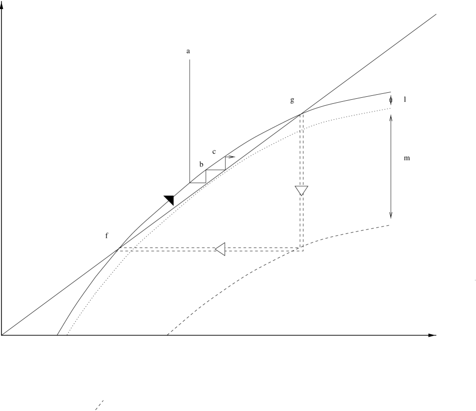
Figure 1: Depiction of the resolution of equation (35) without (subsection (3.1)) and with (subsection (3.2)) a brane source included. Equation (35) defines a sequence which for $\lambda<0$ and small, is characterized by the upper solid curve. The latter curve is representing the function $F_{\lambda}(u)$ which defines the sequence by the recursion relation $f_{i}=F_{\lambda}(f_{i-1})$. The solid oblique line is defined by the function $u=v$. One sees that, when no brane is included, one can only flow (black arrow) from the fixed point $f_{-}$ to the fixed point $f_{+}$, for an “initial” value $f_{0}$ which lies in between the fixed points. This corresponds to the solution (40) and to the negative tension brane discretized bulk. When a brane source is included, one can go “backward” (white arrows and double dashed lines) from the fixed point $f_{+}$ to the fixed point $f_{-}$ at a given value of the index $i$ corresponding to the brane. For this to happen, the brane tension has to be tuned in order for the curve representing $F_{\lambda+2\sigma/3m^{2}M_{(4)}^{2}}$, the dashed bottom curve, to go through the point $(u=f_{+},v=f_{-}$). The solution is then the discretized Randall-Sundrum metric with a positive tension brane. The dotted curve represents the function $F_{0}$. It is tangent to the $u=v$ line at the point $(1,1)$. It also corresponds to the sequence which solution is obtained in equation (57) of subsection 3.3.

3.3 Lapse field and reparametrization invariance

We then turn to another possible discretization of the action (2) keeping the lapse field ${\cal N}$ on all sites. Starting with $V=V_{1}$, the equations of motion now read

$$\sqrt{-\lambda}{\cal N}_{i} = \epsilon_{i}(f_{i}-1),$$ (54)

$$-\lambda{\cal N}_{i} = \frac{1}{{\cal N}_{i}}\left(f_{i}-1\right)-\frac{1}{{\cal N}_{i-1}}\left(1-\frac{1}{f_{i-1}}\right),$$ (55)

where $\epsilon_{i}=\pm 1$. Fixing $\epsilon_{i}$ independently of $i$, and replacing ${\cal N}_{i}$ by its expression as a function of $f_{i}$ given by equation (54) into equation (55), one finds that $f_{i}$ verifies equation (35) with $\lambda=0$, namely

$$-2+f_{i}+\left(f_{i-1}\right)^{-1}=0.$$ (56)

This can be straightforwardly solved to yield

$$g_{\mu\nu}^{i} = I_{0}(i+i_{0})\eta_{\mu\nu},$$ (57)

$${\cal N}_{i}^{2} = \frac{1}{-\lambda(i+i_{0})},$$ (58)

with $i_{0}$ and $I_{0}$ some constants. This exactly reproduces the metric $\tilde{g}_{AB}^{(3)}$, of equation (18) sampled at successive sites $i$ parametrized by their coordinate $z_{i}\equiv ai$ along the $z$ direction. Indeed $g_{\mu\nu}^{i}$ and ${\cal N}_{i}$ as defined by equations (57) and (58) are given by $g_{\mu\nu}^{i}=\tilde{g}^{(3)}_{\mu\nu}(z_{i},x^{\mu})$ and ${\cal N}_{i}^{2}=\tilde{g}^{(3)}_{yy}(z_{i},x^{\mu})$ with the identifications $\tilde{z}_{0}=i_{0}a$ and $Z_{0}=I_{0}/a$. This means in particular that our discretization scheme reproduces, when the discretization step is send to zero, solutions of the 5D continuum theory in a given gauge. This is of course not a surprise, since our discretized action $S[g_{i},{\cal N}_{i}]$ explicitly breaks reparametrization invariance along the $y$ direction. It can also be seen by noticing that, in contrast to the continuum case, the equation of motion of the metric (55) cannot be obtained from the equation of motion for the lapse field (54). This very fact was indeed used to solve for ${\cal N}_{i}$ and $g_{\mu\nu}^{i}$. However, note that both equations reduce to equations (12) and (13) in the leading order in $a$. So that once the solution for ${\cal N}_{i}$ (respectively $g_{\mu\nu}^{i}$) of equations (54-55) is known, which can be considered from the point of view of the continuum theory as setting the gauge, as far as $y$ reparametrization is concerned, then the solution for the $g_{\mu\nu}^{i}$ (respectively ${\cal N}_{i}$) agrees with the solution of the continuum in the small $a$ limit.

Another property of the solution (57,58) is that the parameter $i_{0}$ allows one to avoid the potential singularity which exists in the continuum. In fact if $i_{0}$ is not an integer than the scale factor $a_{i}$ does not vanish for all $i$. This is a generic feature of discretized models.

One can ask whether one can restore the arbitrariness in ${\cal N}_{i}$ by changing the discretization scheme. It turns out indeed to be possible choosing the interaction potential $V$ of $S[g_{i},{\cal N}_{i}]$ to depend on metrics on three adjacent sites, and reading

$$V(g_{i-1},g_{i},g_{i+1})=-{m^{2}\over 16}\sqrt{-g_{i}}\left(g_{\mu\nu}^{i+1}-g_{\mu\nu}^{i-1}\right)\left(g_{\alpha\beta}^{i+1}-g_{\alpha\beta}^{i-1}\right)\left(g_{i}^{\mu\nu}g_{i}^{\alpha\beta}-g_{i}^{\mu\alpha}g_{i}^{\nu\beta}\right).$$ (59)

With this interaction term, the action $S[g_{i},{\cal N}_{i}]$ also agrees with action (2) in the continuum limit. The equations for $\Omega_{i}$ and ${\cal N}_{i}$ now read

$$\Lambda{\cal N}_{i} = \frac{3m^{2}}{8}\left({\Omega_{i}-\Omega_{i+2}\over\Omega_{i}{\cal N}_{i+1}}+{\Omega_{i}-\Omega_{i-2}\over\Omega_{i}{\cal N}_{i-1}}\right)$$ (60)

$$\sqrt{{-\frac{8}{3}\Lambda}}{\cal N}_{i} = \epsilon_{i}m\left({\Omega_{i+1}-\Omega_{i-1}\over\Omega_{i}}\right).$$ (61)

If one chooses the same value of $\epsilon_{i}$ for all $i$, then the first equation is a consequence of the second. It is thus possible to “choose a gauge” by fixing ${\cal N}_{i}$ and then to find $\Omega_{i}$ by solving (61), the resulting solution will automatically satisfy (60). Let us choose, for instance, ${\cal N}_{i}=1=\epsilon_{i}$, then (61) can be readily solved to give a solution depending on two parameters

$$\Omega_{i}=\alpha x_{+}^{i}+\beta x_{-}^{i},$$ (62)

where

$$x_{\pm}=\sqrt{-\lambda}\pm\sqrt{1-\lambda}.$$ (63)

Notice that $x_{-}$ is negative so that the solution with $\alpha=0$ has $\Omega^{i}$ with alternating signs: neighboring spacetimes $i$ and $i+1$ have opposite signatures. This behavior has no continuum counterpart where a singularity is reached before the signature change takes place. When $\beta=0$ the solution coincides, to the first order in $a$ with the solution we found previousely in (37) and so it tends to the $AdS_{5}$ metric in the continuum. Notice that had we started to solve (60) with ${\cal N}_{i}=1$ than we would have obtained the analog of the more general solution (40) but equation (61) would not have been satisfied.

To summarize, the inclusion of ${\cal N}_{i}$ allows to recover just the continuum solutions if we do not insist on having an ${\cal N}_{i}$ undetermined by the equations of motion; and if we do insist, we get extra solutions with no continuum counterpart.

4 Effective 4D gravity

We turn now to determine the gravitational potential without the lapse field, and consider the discretisation scheme given in the previous subsection. We assume here that the cosmological constant vanishes and so we can perturb around flat space-time. To quadratic order in the metric perturbation $h_{\mu\nu}^{i}$, the potential (59) reads

$$V(h_{i-1},h_{i},h_{i+1})=-{m^{2}\over 16}\left(h_{\mu\nu}^{i+1}-h_{\mu\nu}^{i-1}\right)\left(h_{\alpha\beta}^{i+1}-h_{\alpha\beta}^{i-1}\right)\left(\eta^{\mu\nu}\eta^{\alpha\beta}-\eta^{\mu\alpha}\eta^{\nu\beta}\right).$$ (64)

In order to diagonalize this interaction, we define $\check{h}_{\mu\nu}$ by

$$\check{h}_{\mu\nu}\left(x^{\alpha},\theta\right)=\sum_{n}h^{n}_{\mu\nu}(x^{\alpha})e^{in\theta}.$$ (65)

The quadratic action is then an integral over $\theta$ of Pauli-Fierz actions with a continuous mass spectrum given by

$$m^{2}(\theta)={\sin^{2}\theta\over a^{2}}.$$ (66)

And the gravitational potential $\Psi_{j}(r)$, between two unit masses separated by $r$ and placed at sites $i$ and $i+j$, can be obtained summing over Pauli-Fierz propagators. The outcome of the calculation can also be simply understood from discretizing the Laplacian equation with the same discretization scheme as above. The discretized equation reads

$$\partial^{2}\Psi_{j}+{{(\Psi_{j+2}+\Psi_{j-2}-2\Psi_{j})}\over 4a^{2}}=4\pi G_{N}\delta(\bf r)\delta_{j,0},$$ (67)

where we have reintroduced the Newton constant $G_{N}$. The Fourier transform $\check{\Psi}$, as defined above, verifies

$$\partial^{2}\check{\Psi}(r,\theta)-m^{2}(\theta)\check{\Psi}(r,\theta)=4\pi G_{N}\delta(\bf r).$$ (68)

Notice that the mass spectrum is bounded from above by the inverse lattice spacing $a^{-1}$. A continuous mass spectrum is reminiscent of the infinite dimensional models of [19, 20]. The gravitational potential can now be readily put in the form

$$\Psi_{j}(r)=-{G_{N}\over r}\int_{0}^{\pi}{d\theta\over{\pi}}e^{-{r\over a}\sin\theta}\cos j\theta.$$ (69)

When $r<<a$ then the integral can be approximated by $\delta_{j,0}$ and the potential reduces to the 4D Newtonian potential

$$\Psi_{j}(r)=-{G_{N}\over r}\left(\delta_{j,0}+O({r\over a})\right),\ \ \ r<<a.$$ (70)

When $r>>a$, then the integral can be approached by

$$\int_{0}^{\pi/2}{d\theta\over{\pi}}e^{-{r\over a}\theta}\cos j\theta+\int_{\pi/2}^{\pi}{d\theta\over{\pi}}e^{-{r\over a}(\pi-\theta)}\cos j\theta={1\over\pi a}{r\over{r^{2}+a^{2}j^{2}}}(1+(-1)^{j}+O(e^{-r\over a})),$$

so that the gravitational potential is of the form of a 5D potential

$$\Psi_{j}(r)=-{G_{5}\over r^{2}+(ja)^{2}},$$ (71)

if $j$ is even, with the 5D gravitational constant being given by

$$G_{5}={2G_{N}\over{\pi a}}.$$ (72)

When $j$ is odd the gravitational potential is exponentially small. Gravity is thus four dimensional at small length scales and five dimensional at large scales. Choosing $a$ very large (of the order of the Hubble scale) allows a very simple modification of gravity at large scales in the spirit of the models of references [18, 19, 20, 21]. Note that we could have started from a finite number $N$ of sites. This corresponds to an extra dimension which is compact with a length scale $R=Na$. The graviton spectrum would have been discrete with a spacing of order $1/N$ and would have remained bounded. In this case, the four dimensional regime is obtained both for small scales $r<<a$ and large scales $r>>R$, the intermediate scales being five dimensional $a<<r<<R$. The qualitative features of this potential are not sensitive to the particular form of the discretization scheme we have used. On the other hand, it is well known that the tensorial structure of the propagator of massive spin 2 fields differs dramatically from the massless one. This leads to the vDVZ discontinuity at the linearized level which is manifested by, e.g., an order one difference in light bending. In this respect, when $R$ is infinite we expect the discontinuity to be present since we have a continuous spectrum of massive gravitons. This is similar to the brane models with an extra infinite dimension [18, 19, 20, 21]. When $R$ is finite, however, the spectrum is discrete and there is no discontinuity.

5 Cosmological solutions

The discussion of preceeding subsections enables to find easily some cosmological solutions for the type of models considered here. It is the purpose of this last section to discuss those solutions. We look for solutions where the line element of site $i$ takes the form

$$ds^{2}_{i}=-B_{i}^{2}(t)dt^{2}+A_{i}^{2}(t)d\vec{x}^{2}.$$ (73)

The equations of motion derived from action (24) (where we consider ${\cal N}_{i}$ as a non dynamical field set to $1$) with the potential $V_{1}$ read

$$3{\dot{A}_{i}^{2}\over A_{i}^{2}}-\tilde{\Lambda}B_{i}^{2} = -\frac{3B_{i}^{2}}{2a^{2}}\left\{1+\frac{B^{2}_{i+1}}{2B^{2}_{i}}-\frac{A^{2}_{i+1}B^{2}_{i+1}}{2A^{2}_{i}B^{2}_{i}}-\frac{3A^{2}_{i+1}}{2A^{2}_{i}}+\frac{A_{i+1}^{4}}{2A^{4}_{i}}\right\}$$ (74)

$$-\frac{3B_{i}^{2}}{2a^{2}}\left\{\frac{B_{i}}{A_{i}}\frac{A_{i-1}}{B_{i-1}}\left(\frac{A^{2}_{i}-A^{2}_{i-1}}{A^{2}_{i}}\right)\right\}+M_{(4)}^{-2}B^{2}_{i}\rho_{i},$$

$$-{\dot{A}_{i}^{2}\over A_{i}^{2}}-2{\ddot{A}_{i}\over A_{i}}+2{\dot{A}_{i}\dot{B}_{i}\over A_{i}B_{i}}+\tilde{\Lambda}B_{i}^{2} = -\frac{B_{i}^{2}}{2a^{2}A_{i}^{2}}\left\{-\frac{B^{2}_{i+1}A^{2}_{i+1}}{2B_{i}^{2}}+\frac{A_{i+1}^{4}}{2A^{2}_{i}}+\frac{3}{2}A^{2}_{i+1}-3A_{i}^{2}+\frac{3B_{i+1}^{2}A^{2}_{i}}{2B^{2}_{i}}\right.$$ (75)

$$\left.-A_{i}^{2}\frac{A_{i-1}B_{i-1}}{A_{i}B_{i}}\left(\frac{B^{2}_{i}}{B^{2}_{i-1}}+2\frac{A^{2}_{i}}{A^{2}_{i-1}}-3\right)\right\}+M_{(4)}^{-2}p_{i}B_{i}^{2},$$

where we have included the possibility for each site $i$ to host matter with energy density $\rho_{i}$ and pressure $p_{i}$ (that is to say, matter, in the form of a perfect fluid, is assumed to be confined on each site). We then look for factorized solutions of the form

$$A^{2}_{i}(t) = \alpha_{i}A^{2}(t),$$

$$B_{i}^{2}(t) = \beta_{i}B^{2}(t),$$ (76)

where $\alpha_{i}$ and $\beta_{i}$ are time-idependent, we also set $B$ to one by a suitable time redefinition. We then further simplify the problem by letting $\alpha_{i}=\beta_{i}$, and look for solution where the metric on each site is de Sitter, and the sites are only endowed with a cosmological constant $\sigma$. This means $\rho_{i}$ obeyes $\rho_{i}=-p_{i}=\sigma$ and does not depend on $i$. In this case, the equations of motion reduce to

$$\frac{\dot{A}^{2}}{A^{2}} = H^{2},$$

$$\frac{3}{2a^{2}}\left(\alpha_{i+1}+\alpha_{i-1}-2\alpha_{i}\right) = 3H^{2}-\left(\tilde{\Lambda}+M_{(4)}^{-2}\sigma\right).$$ (77)

These equations can easily be solved. Let us first discuss the case where $(\tilde{\Lambda}+M_{(4)}^{-2}\sigma)$ does not vanish. In this case, defining $\gamma$ by $\gamma=3H^{2}/\left(\tilde{\Lambda}+M_{(4)}^{-2}\sigma\right)$, the sequence $f_{i}\equiv(\alpha_{i+1}-\gamma)/(\alpha_{i}-\gamma)$ obeyes equation (35) with $\lambda$ given by $\lambda\equiv 2(\tilde{\Lambda}+M_{(4)}^{-2}\sigma)a^{2}/3$. So that the solutions are readily obtained from those of section 3. In the case where $(\tilde{\Lambda}+M_{(4)}^{-2}\sigma)$ vanishes, on the other hand, the solution to equation (77) is given by

$$\alpha_{i}=\alpha_{0}+\tilde{\alpha}_{0}i+H^{2}a^{2}i^{2},$$ (78)

where $\alpha_{0}$ and $\tilde{\alpha}_{0}$ are some arbitrary constants. Interestingly, this solution has de Sitter 4D space-time on each sites, but vanishing cosmological constants. This is in analogy with what is happening in the brane-induced gravity model [22, 11] as is the behavior of the Newtonian gravitationnal potential that was discussed in the preceeding section. However in contrast to brane-induced gravity, the curvature of de Sitter space-time is here arbitrary. Note that, had we kept the $X^{\mu}_{i}$ fields as a dynamical variables, one should have also considered their equations of motion. The latter, for the ansatz (76), reduce to

$${\dot{A}\over A}\left(2{\alpha_{i+1}\over\alpha_{i}}-3\right)\left({\alpha_{i+1}\over\alpha_{i}}-{\beta_{i+1}\over\beta_{i}}\right)=0.$$ (79)

This equation is satisfied for our choice $\alpha_{i}=\beta_{i}$. However, in a similar way as was discussed previously, solution (78) does not verify (for $H\neq 0$) the equations of motion for ${\cal N}_{i}$ which reads (for ${\cal N}_{i}=1$)

$$\frac{6}{\alpha_{i}}\left(\frac{\dot{A}^{2}}{A^{2}}+\frac{\ddot{A}}{A}\right)=\frac{3}{a^{2}}\left(\frac{\alpha_{i+1}-\alpha_{i}}{\alpha_{i}}\right)^{2}.$$ (80)

Indeed in the continuum theory, there is no solution equivalent to (78) with arbitrary $\alpha_{0}$ and $\tilde{\alpha}_{0}$; rather one finds a related solution describing a slicing of 5D Minkowski space-time by 4D de Sitter space-times which reads

$$ds^{2}=(1+Hy)^{2}\left(-dt^{2}+e^{2Ht}d\vec{x}\right)+dy^{2}.$$ (81)

This solution is conveniently used to described the space-time on one side of a domain-wall, which entire space time is given by the above solution where $y$ is replaced by $|y|$ [23].

6 Conclusions

In this paper, we have investigated some exact solutions of 5D General Relativity with a discrete fifth dimension, and compared them to solutions of the continuum theory. Depending on the discretization scheme used, we have shown that some of the solutions of the discrete theory exactly match those of the continuum, while others do not. In general, the discretization explicitly breaks reparametrization along the discrete dimension. This gets reflected in the fact that for solution we have considered, corresponding to slicing of $AdS_{5}$ by Minkowski space, the equations of motion of the discrete theory enable in general to determine both the lapse field and the 4D metric. This is to be contrasted with the continuum theory, where the lapse field cannot be determined by the equations of motion. However, we have shown that one can find a given discretization scheme in which it remains undetermined. More importantly, some of the solutions of the discrete theory exibit very dramatic differences with those of the continuum. As shown here, one can find signature change of the 4D metric but also avoidance of singularities which would be present in the continuum. In addition we have also found a brane world looking bulk space time, with no brane source in the equation of motion and no fine tuning. This solution would correspond in the continuum theory to a negative tension brane. We investigated the static gravitational potential and found it realistic when the lattice spacing is very large. Last, we also discussed some cosmological solutions.

We can look at our results from two different perspectives. On one hand, they exemplify the difficulties which arise upon deconstruction of gravity even at the classical level: the neglect of the lapse fields leads to spurious solutions, while their inclusion only partially solves this problem, as we showed in section 3. On the other hand, they point out interesting directions in multigravity theories: they allow, as we showed, simple modifications of gravity at large scales and brane-like solutions with no branes. One can speculate on the possibility to reproduce these results, in some more complex multigravity, without the various drawbacks mentioned in the introduction. It would also be interesting to find a solution corresponding to the discretization of RS type - gravity localizing - metric [1], and at the same time avoiding fine tuning conditions.

References

- [1] L. Randall and R. Sundrum, Phys. Rev. Lett. 83 (1999) 3370 [arXiv:hep-ph/9905221]. L. Randall and R. Sundrum, Phys. Rev. Lett. 83 (1999) 4690 [arXiv:hep-th/9906064]. for a review see V. A. Rubakov, “Large and infinite extra dimensions: An introduction,” Phys. Usp. 44, 871 (2001) [Usp. Fiz. Nauk 171, 913 (2001)] [arXiv:hep-ph/0104152].
- [2] M. Fierz and W. Pauli, Proc. Roy. Soc. Lond. A 173 (1939) 211.
- [3] C. J. Isham, A. Salam and J. Strathdee, Phys. Rev. D 3 (1971) 867. A. Salam and J. Strathdee, Phys. Rev. D 16, 2668 (1977). C. J. Isham and D. Storey, Phys. Rev. D 18, 1047 (1978). A. H. Chamseddine, Phys. Lett. B 557, 247 (2003) [arXiv:hep-th/0301014].
- [4] D. G. Boulware and S. Deser, Phys. Rev. D 6 (1972) 3368.
- [5] T. Damour and I. I. Kogan, Phys. Rev. D 66 (2002) 104024 [arXiv:hep-th/0206042]. T. Damour, I. I. Kogan and A. Papazoglou, Phys. Rev. D 66, 104025 (2002) [arXiv:hep-th/0206044]. T. Damour, I. I. Kogan and A. Papazoglou, Phys. Rev. D 67, 064009 (2003) [arXiv:hep-th/0212155].
- [6] N. Arkani-Hamed, H. Georgi and M. D. Schwartz, Annals Phys. 305 (2003) 96 [arXiv:hep-th/0210184]. N. Arkani-Hamed and M. D. Schwartz, arXiv:hep-th/0302110; M. D. Schwartz, arXiv:hep-th/0303114.
- [7] N. Arkani-Hamed, A. G. Cohen and H. Georgi, Phys. Rev. Lett. 86 (2001) 4757 [arXiv:hep-th/0104005]. C. T. Hill, S. Pokorski and J. Wang, Phys. Rev. D 64 (2001) 105005 [arXiv:hep-th/0104035].
- [8] J. Madore, Phys. Rev. D 41, 3709 (1990); J. Madore and J. Mourad, Class. Quant. Grav. 10 (1993) 2157. J. Madore and J.Mourad, “Noncommutative Kaluza-Klein Theory,” arXiv:hep-th/9601169 and references therein.
- [9] H. van Dam and M. J. Veltman, Nucl. Phys. B 22 (1970) 397. V.I.Zakharov, JETP Lett 12, 312 (1970). Y. Iwasaki, Phys. Rev. D 2 (1970) 2255.
- [10] M. A. Luty, M. Porrati and R. Rattazzi, arXiv:hep-th/0303116. V. A. Rubakov, arXiv:hep-th/0303125.
- [11] C. Deffayet, Phys. Lett. B 502 (2001) 199 [arXiv:hep-th/0010186]. C. Deffayet, G. R. Dvali and G. Gabadadze, Phys. Rev. D 65 (2002) 044023 [arXiv:astro-ph/0105068].
- [12] A. I. Vainshtein, Phys. Lett. B 39 (1972) 393. C. Deffayet, G. R. Dvali, G. Gabadadze and A. I. Vainshtein, Phys. Rev. D 65 (2002) 044026 [arXiv:hep-th/0106001]. A. Lue, Phys. Rev. D 66 (2002) 043509 [arXiv:hep-th/0111168]. A. Gruzinov, arXiv:astro-ph/0112246. M. Porrati, Phys. Lett. B 534 (2002) 209 [arXiv:hep-th/0203014]. T. Tanaka, arXiv:gr-qc/0305031.
- [13] L. Dolan and M. J. Duff, Phys. Rev. Lett. 52 (1984) 14. C. S. Aulakh and D. Sahdev, Phys. Lett. B 164 (1985) 293. C. R. Nappi and L. Witten, Phys. Rev. D 40 (1989) 1095.
- [14] C. Deffayet, J. Mourad, Multigravity from a discete extra dimension hep-th/0311124
- [15] P. Jordan, Ann. Phys. (Leipzig 1947). Y. Thiry, CRAS, 216 (1948).
- [16] M. J. Duff, B. E. Nilsson, C. N. Pope and N. P. Warner, Phys. Lett. B 149 (1984) 90.
- [17] P. Binétruy, C. Deffayet and D. Langlois, Nucl. Phys. B 565 (2000) 269 [arXiv:hep-th/9905012].
- [18] I. I. Kogan, S. Mouslopoulos, A. Papazoglou, G. G. Ross and J. Santiago, Nucl. Phys. B 584, 313 (2000) [arXiv:hep-ph/9912552].
- [19] R. Gregory, V. A. Rubakov and S. M. Sibiryakov, Phys. Rev. Lett. 84, 5928 (2000) [arXiv:hep-th/0002072].
- [20] G. R. Dvali, G. Gabadadze and M. Porrati, Phys. Lett. B 484, 112 (2000) [arXiv:hep-th/0002190].
- [21] I. I. Kogan and G. G. Ross, Phys. Lett. B 485, 255 (2000) [arXiv:hep-th/0003074].
- [22] G. R. Dvali, G. Gabadadze and M. Porrati, Phys. Lett. B 485, 208 (2000) [arXiv:hep-th/0005016].
- [23] A. Vilenkin, Phys. Lett. B 133 (1983) 177. J. Ipser and P. Sikivie, Phys. Rev. D 30, 712 (1984).