Tachyons, Scalar Fields and Cosmology

Abstract

We study the role that tachyon fields may play in cosmology as compared to the well-established use of minimally coupled scalar fields. We first elaborate on a kind of correspondence existing between tachyons and minimally coupled scalar fields; corresponding theories give rise to the same cosmological evolution for a particular choice of the initial conditions but not for any other. This leads us to study a specific one-parameter family of tachyonic models based on a perfect fluid mixed with a positive cosmological constant. For positive values of the parameter one needs to modify Sen’s action and use the $\sigma$-process of resolution of singularities. The physics described by this model is dramatically different and much richer than that of the corresponding scalar field. For particular choices of the initial conditions the universe, that does mimick for a long time a de Sitter-like expansion, ends up in a finite time in a special type of singularity that we call a big brake. This singularity is characterized by an infinite deceleration.

I Introduction

The recently discovered cosmic acceleration accel1 ; accel2 ; accel3 has put forward the problem of unravelling the nature of the so called dark energy responsible for such phenomenon (for a review see Star-Varun ; Pad-rep ). The crucial feature of the dark energy which ensures an accelerated expansion of the universe is that it breaks the strong energy condition.

The tachyon field arising in the context of string theory Sen ; Sen1 ; Sen2 ; Garousi provides one example of matter which does the job. The tachyon has been intensively studied during the last few years also in application to cosmology Gibbons1 –bilbao1 ; in this case one usually takes Sen’s effective action Sen for granted and studies its cosmological consequences without worrying about the string-theoretical origin of the action itself. We take this attitude in the present paper.

However, it would be reasonable, before considering concrete tachyon cosmological models, to answer a simple question: is the tachyon field of real interest for cosmology? Indeed, it is well-known that for isotropic cosmological models, for a given dependence of the cosmological radius on time it is always possible to construct a potential for a minimally coupled scalar field (in brief: scalar field) model, which would reproduce this cosmological evolution (see e.g. Star-scal ), provided rather general reasonable conditions are satisfied. Since a similar statement holds also for cosmological models with tachyons, one can find some kind of correspondence between minimally coupled scalar field models and tachyon ones describing the same cosmological evolution Padman . Therefore, a natural question arises: does it make sense at all to study tachyon cosmological models in place of the traditional scalar field models?

In our opinion, the point is that the correspondence between tachyon and scalar field cosmological models is a rather limited one and amounts to the existence of ”corresponding” solutions of the models, obtained by imposing certain special initial conditions. If one moves away from these conditions the dynamics of the tachyon model can become more complicated and very different from that of its scalar field cousin.

In this paper we consider some examples of scalar and tachyon field isotropic cosmological models having coincident exact solutions. All the exact solutions considered here actually arise as solutions of some isotropic perfect fluid cosmological models.

Some of the tachyon and scalar field potentials that we consider here are well known in the literature and are widely used as quintessential models. We will introduce also a new (at least to our knowledge) tachyon model that is based on the cosmic evolution driven by the mixture of a cosmological constant and of a fluid with equation of state $p=k\varepsilon$, with $-1<k\leq 1$ ($\varepsilon$ and $p$ denote as usual the energy density and the pressure respectively). The corresponding tachyon potential $V(T)$ is represented by a rather cumbersome trigonometric function of the tachyon field. When the parameter $k$ is positive the potential becomes imaginary passing through zero for finite values of the tachyon field $T$. Thus, it might seem that these features would kill the model; on the contrary, using the methods of the qualitative theory of ordinary differential equations, it is possible to extract from the model a dynamics which is perfectly meaningful also for positive $k$. We find that this dynamics is quite rich. In particular, when the value of the parameter $k$ is positive, the model possesses two types of trajectories: trajectories describing an eternally expanding universe and those hitting a cosmological singularity of a special type that we have chosen to call a big brake. Thus, starting with a simple perfect fluid model and trying to reproduce its cosmological evolution in scalar field and tachyon models, we arrive to a relatively simple scalar field potential with a correspondingly simple dynamics and to a complicated tachyon potential. The latter provides us with a model having a very interesting dynamics giving rise to very different cosmological evolutions and opening in turn opportunities for some non-trivial speculations about the future of the universe.

The structure of the paper is as follows. In the second section we study the problem of the correspondence between tachyon and scalar field cosmological models and give some examples in the third section. In the fourth section we suggest a way to go beyond the limitations of tachyonic models and we make use of this idea in the fifth and sixth sections where we study the dynamics and the cosmology of a particular (toy) tachyon model introduced in Sec. 3. In the last section we conclude our paper by some speculations on the future evolution of the universe arising from the analysis of our model.

II The correspondence

We consider a flat Friedmann cosmological model $ds^{2}=dt^{2}-a^{2}(t)dl^{2}$ of a universe filled with some perfect fluid and suppose that the cosmological evolution $a=a(t)$ is given; the Friedmann equation

$$\frac{\dot{a}^{2}}{a^{2}}=\varepsilon$$ (1)

provides the dependence $\varepsilon=\varepsilon(t)$ of the energy density of the fluid on the cosmic time (we have put $8\pi G/3=1$ for convenience). Then, the equation for energy conservation

$$\dot{\varepsilon}=-3\frac{\dot{a}}{a}(\varepsilon+p)$$ (2)

fixes the pressure $p=p(t)$; therefore an equation of state $p=p(\varepsilon)$ can in principle be written describing the unique fluid model compatible with the given cosmic evolution (provided that $\dot{\varepsilon}\not=0$).

Now, let us suppose that the matter content of the universe is modeled by a homogeneous tachyon field $T(t)$ described by Sen’s Lagrangian density Sen ; Sen1 :

$$L=-V(T)\sqrt{1-{\dot{T}}^{2}}.$$ (3)

The energy momentum tensor is diagonal and the corresponding field-dependent energy density and pressure are given by

$$\varepsilon=\frac{V(T)}{\sqrt{1-\dot{T}^{2}}},$$ (4)

$$p=-V(T)\sqrt{1-\dot{T}^{2}},$$ (5)

while the field equation for the tachyon is written as follows

$$\frac{\ddot{T}}{1-\dot{T}^{2}}+\frac{3\dot{a}{\dot{T}}}{a}+\frac{V_{,T}}{V}=0.$$ (6)

One can try and find a potential $V(T)$ so that, for certain suitably chosen initial conditions on the tachyon field, the scale factor of the universe is precisely the given $a(t)$. A similar construction can be attempted for a minimally coupled scalar field, described by the Lagrangian density

$$L=\frac{1}{2}\dot{\varphi}^{2}-U(\varphi).$$ (7)

A given cosmological evolution $a=a(t)$ can therefore be used to establish a sort of correspondence between the two potentials $V(T)$ and $U(\varphi)$ (see also Padman ).

Let us see in some detail how this works and what the sought correspondence really means. It is often more practical to use the scale factor $a$ to parameterize the cosmic time; this can be done provided $\dot{a}\not=0$. From Eqs. (4) and (5) it follows that

$${\dot{T}}^{2}=\frac{p+\varepsilon}{\varepsilon}.$$ (8)

By using Eqs. (1) and (2) the latter equation can be rewritten as follows

$$T^{\prime}=\frac{1}{a}\sqrt{\frac{(\varepsilon+p)}{\varepsilon^{2}}}=\frac{1}{a}\sqrt{\frac{-\varepsilon^{\prime}a}{3\varepsilon^{2}}}$$ (9)

where “prime” denotes the derivative with respect to $a$. Once $a(t)$ and therefore $\varepsilon(a)$ is specified (see Eq. (1)), Eq. (9) can be integrated to give

$$T=\Phi(a)=\int^{a}\frac{dx}{x}\sqrt{\frac{-\varepsilon^{\prime}(x)\,x}{3\varepsilon^{2}(x)}}$$ (10)

(an arbitrary additive integration constant is hidden in the unspecified integration limit). By inverting Eq.(10) $a=\Phi^{-1}(T)$ and making use of the relation

$$V=\sqrt{-\varepsilon p}=\sqrt{\frac{(\varepsilon^{2}a^{6})^{\prime}}{6a^{5}}},$$ (11)

the shape of the required tachyon potential $V=V(a)=V(\Phi^{-1}(T))$ can be found.

For the minimally coupled scalar field we have similar formulas. The analogs of Eqs. (4) and (5) for the scalar field are

$$\varepsilon=\frac{1}{2}\dot{\varphi}^{2}+U(\varphi),$$ (12)

$$p=\frac{1}{2}\dot{\varphi}^{2}-U(\varphi).$$ (13)

From these we get

$$\varphi^{\prime}=\frac{1}{a}\sqrt{\frac{(\varepsilon+p)}{\varepsilon}}=\frac{1}{a}\sqrt{\frac{-\varepsilon^{\prime}a}{3\varepsilon}}$$ (14)

and

$$U=\frac{1}{2}(\varepsilon-p)=\frac{(\varepsilon a^{6})^{\prime}}{6a^{5}}.$$ (15)

Integration of Eq. (14) gives

$$\varphi=F(a)=\int^{a}\frac{dx}{x}\sqrt{\frac{-\varepsilon^{\prime}(x)\,x}{3\varepsilon(x)}}$$ (16)

and as before $U=U(a)=U(F^{-1}(\varphi))$. The formulas above establish a kind of correspondence between the potentials $U$ and $V$ in the sense that the cosmologies resulting from such potentials admit the given cosmological evolution $a=a(t)$ for suitably chosen initial conditions on the fields. However, it has to be stressed that for arbitrary initial conditions on the fields the cosmological evolutions (within the corresponding models) may be drastically different. Furthermore, changing the initial conditions, say, for a minimally coupled scalar field theory, one gets different cosmological evolutions which, in turn, can be reproduced in entirely different tachyon theories and viceversa. Thus, any scalar field potential has a whole (one-parameter) family of corresponding tachyon potentials and the same is true the other way around.

We can learn something more by expressing the fields $T$ and $\varphi$ and the potentials $V(T)$ and $U(\varphi)$ in terms of the Hubble variable $h=\dot{a}/a$. Since

$$\dot{h}=-\frac{3}{2}(\varepsilon+p)$$ (17)

one has easily that

$$\dot{T}^{2}=\frac{\varepsilon+p}{\varepsilon}=-\frac{2\dot{h}}{3h^{2}},\;\;\;\;\;\;V(T)=\sqrt{h^{2}\left(\frac{2}{3}\dot{h}+h^{2}\right)},$$ (18)

and that

$$\dot{\varphi}^{2}=\varepsilon+p=-\frac{2}{3}\dot{h},\;\;\;\;\;\;U(\varphi)=h^{2}+\frac{1}{3}\dot{h}.$$ (19)

Eqs. (18) and (19) call for the condition $\varepsilon+p\geq 0,$ or equivalently $\dot{h}\leq 0$. For the tachyon model Eq. (18) requires the additional condition

$$\dot{h}\geq-\frac{3}{2}h^{2}$$ (20)

which is equivalent to ask for a negative pressure $p\leq 0$. It seems therefore that tachyonic models are more restrictive than minimally coupled scalar fields in their possibility to describe cosmological evolutions. We will see in an example that this seemingly negative conclusion can be overcome and pleasant surprises may arise.

III Examples

We now illustrate the above considerations by means of some explicitly solvable examples. In these examples we assume, as usual, that the initial moment of time, $t=0$, corresponds to the cosmological singularity. All these examples are based on simple models of perfect fluids as specified by their equations of state.

1. The starting point of the first example is a model of universe filled with a perfect fluid with equation of state $p=k\varepsilon$, with $-1<k\leq 1$; the Hubble variable of this model is given by

   $$h(t)=\frac{2}{3(1+k)t}.$$ (21)

   A minimally coupled scalar field theory that produces the same evolution $h(t)$ for suitably chosen initial conditions can be based on one of the following scalar potentials, which are obtained by the procedure outlined in the previous section:

   $$U_{\pm}(\varphi)=\frac{2}{9}\,\frac{1-k}{(1+k)^{2}}\ e^{\pm 3\sqrt{1+k}(\varphi-\varphi_{0})};$$ (22)

   the limiting case $k=1$ gives a minimally coupled massless field. For $k>1$ the potential becomes negative reflecting the fact that the velocity of sound is bigger than the speed of light.

   Both choices of sign in the exponent are acceptable and the normalization of the potentials can be chosen arbitrarily (the constant $\varphi_{0}$); then, the exact solutions of the field equations providing the prescribed cosmological evolution (21) are, respectively, the following:

   $$\varphi_{\pm}(t)=\mp\frac{2}{3\sqrt{1+k}}\ln t+\varphi_{0}.$$ (23)

   The theories are obviously connected by the symmetry operation $\varphi-\varphi_{0}\rightarrow-(\varphi-\varphi_{0})$, which exchanges the potentials and the corresponding solutions.

   To construct a tachyonic field theory we have to restrict our attention to the case $p<0$, i.e. $k<0$. Following the same procedure we get a tachyon field model, based on the potential

   $$V(T)=\frac{4}{9}\ \frac{\sqrt{-k}}{(1+k)}\ \frac{1}{(T-T_{0})^{2}}.$$ (24)

   There are again two exact solutions of the field equations (21), which now do co-exist within the same model:

   $$T_{\pm}(t)=\pm\sqrt{1+k}\ t+T_{0}.$$ (25)

   This tachyonic model has been studied in Feinstein ; Padman , where also the correspondence with a minimally coupled scalar field theory with exponential potential was noticed. There exists a vast literature on the latter (see e.g. matarrese -Napoli ).

2. Now we add a positive cosmological constant to the previous model, i.e. we consider the mixture

   $$p_{1}=k\varepsilon_{1},\ -1<k\leq 1,\,\,p_{\Lambda}=-\varepsilon_{\Lambda}=-\Lambda,\ \ \ \Lambda>0.$$ (26)

   This is the same as one fluid with state equation

   $$p=k\varepsilon-(1+k)\Lambda.$$ (27)

   The evolution of the Hubble variable is now given by

   $$h(t)=\sqrt{\Lambda}\coth\frac{3\sqrt{\Lambda}(1+k)t}{2}.$$ (28)

   The corresponding minimally coupled scalar field theory is based on the following potential:

   $$U(\varphi)=\Lambda\left(1+\frac{1-k}{2}\sinh^{2}\frac{3\,\sqrt{1+k}\,(\varphi-\varphi_{0})}{2}\right).$$ (29)

   There are two exact solutions of the field equations reproducing the given cosmic evolution (28):

   $$\varphi_{\pm}(t)=\pm\frac{2}{3\sqrt{1+k}}\ \ln\ \tanh\frac{3\sqrt{\Lambda}(1+k)t}{4}+\varphi_{0}.$$ (30)

   To find the tachyonic model we observe first of all that to have the restriction $p<0$ satisfied it is sufficient to require that $-1<k\leq 0$; this condition is also necessary if one demands that $p<0$ during all the stages of the cosmological evolution and for any choice of the initial conditions in the tachyonic model. With this condition we obtain the following more complicated tachyon potential:

   $$V(T)=\frac{\Lambda}{\sin^{2}\left[\frac{3}{2}{\sqrt{\Lambda\,(1+k)}\ (T-T_{0})}\right]}\sqrt{1-(1+k)\cos^{2}\left[\frac{3}{2}{\sqrt{\Lambda\,(1+k)}\,(T-T_{0})}\right]}.$$ (31)

   Still, the corresponding exact solutions can be found and are given by

   $$T(t)=\pm\frac{2}{3\sqrt{\Lambda(1+k)}}\arctan\sinh\frac{3\sqrt{\Lambda}(1+k)t}{2}+T_{0}.$$ (32)

   For $k>0$ there are values of the tachyon field for which the potential (31) becomes imaginary passing through zero.

   When $\Lambda$ tends to zero one expects to recover the model studied in the first example. This is indeed the case for the tachyonic field.

   As for the scalar potential (29) the situation is a bit trickier: the correct limit can be obtained only by letting the constant $\varphi_{0}$ vary with $\Lambda$ as follows:

   $$\varphi_{02}=\varphi_{01}\pm\frac{1}{3\sqrt{1+k}}\ln\frac{\Lambda(1-k)}{2},$$ (33)

   where the subscripts 1 and 2 refer to the corresponding examples. This is because the theory has a symmetry which is lost in the limit.

   Notice that the scalar field potential (29) is well-defined at $-1<k\leq 1$ and the model possesses the exact solution (30) which corresponds to the cosmological evolution (28). The dynamics of the universe within the tachyonic models (24) and (31) will be studied in detail in the next sections for general initial conditions. We shall show that both models can be extended to the interval $0<k\leq 1$, actually making them richer than the corresponding scalar minimally coupled theories.
   

3. In the third example we consider a perfect fluid whose equation of state is as follows:

   $$\varepsilon+p=\gamma\varepsilon^{\lambda},\,\ \ \ 0<\gamma<1,\,\ \ \ \lambda>1.$$ (34)

   In this case the Hubble variable is

   $$h(t)=\left(\frac{3}{2}\,\gamma\ (2\lambda-1)\,t\right)^{\frac{1}{1-2\lambda}}.$$ (35)

   The scalar potential has the form

   $$U(\varphi)=\left(\frac{3\sqrt{\gamma}(\lambda-1)(\varphi-\varphi_{0})}{2}\right)^{-\frac{2}{\lambda-1}}-\frac{\gamma}{2}\left(\frac{3\sqrt{\gamma}(\lambda-1)(\varphi-\varphi_{0})}{2}\right)^{-\frac{2\lambda}{\lambda-1}}.$$ (36)

   The exact solutions are

   $$\varphi(t)=\pm\sqrt{\gamma}\frac{1-2\lambda}{1-\lambda}\left(\frac{3}{2}\gamma(2\lambda-1)t\right)^{\frac{1-\lambda}{1-2\lambda}}+\varphi_{0}.$$ (37)

   The tachyon potential is

   $$V(T)=\sqrt{\left(\frac{3\sqrt{\gamma}\lambda(T-T_{0})}{2}\right)^{-\frac{4}{\lambda}}-\gamma\left(\frac{3\sqrt{\gamma}\lambda(T-T_{0})}{2}\right)^{-\frac{2(1+\lambda)}{\lambda}}},$$ (38)

   with the following exact solutions:

   $$T(t)=\pm\sqrt{\gamma}\frac{2\lambda-1}{\lambda}\left(\frac{3}{2}\gamma(2\lambda-1)t\right)^{\frac{-\lambda}{1-2\lambda}}+T_{0}.$$ (39)

   The scalar field model with the potential (36) was studied in Barrow2 while the corresponding tachyon model with the potential (38) was discussed in Feinstein ; Padman .
   

4. In our last example we consider the Chaplygin gas, described by the following equation of state:

   $$p=-\frac{A}{\varepsilon},\ A>0.$$ (40)

   In this example the evolution $h(t)$ is given only implicitly we by the formula:

   $$t=\frac{1}{6A^{1/4}}\left(\ln\frac{h+A^{1/4}}{h-A^{1/4}}-2\arctan\frac{h}{A^{1/4}}+\pi\right),$$ (41)

   However, as shown in we , the scalar potential can be reconstructed using the known explicit dependence of $\varepsilon$ on $a$ and one gets

   $$U(\varphi)=\frac{1}{2}\sqrt{A}\left(\cosh 3(\varphi-\varphi_{0})+\frac{1}{\cosh 3(\varphi-\varphi_{0})}\right).$$ (42)

   The corresponding field configuration is also given implicitly:

   $$\varphi(t)=\mp\frac{1}{3}{\rm arccosh}\left(\frac{\left(h^{2}(t)+\frac{\dot{h}(t)}{3}\right)}{\sqrt{A}}+\sqrt{\frac{\left(h^{2}(t)+\frac{\dot{h}(t_{0})}{3}\right)^{2}}{A}-1}\right)+\varphi_{0}.$$ (43)

   Similarly, using the dependence of $\varepsilon$ on $a$ one can reconstruct the tachyon potential:

   $$V(T)=\sqrt{A}=const.$$ (44)

   It is easy to see FKS that the tachyon model with a constant potential is exactly equivalent to the Chaplygin gas model. Indeed, in the case of a constant tachyon potential the relation between the tachyon energy density (4) and the pressure (5) is just that of the Chaplygin gas (40), where $p\ \varepsilon=-V^{2}(T)=-A$. The Chaplygin gas cosmological model was introduced in we and further developed in Fabris ; Bilic ; Bento ; we1 and many other papers. Comparison with observational data has also been extensively performed Chap-obs .

IV Transgressing the boundaries

We now take a step back and consider the problem of finding a tachyonic field theory admitting the same cosmic evolution as the one produced by perfect fluid with equation of state $p=k\varepsilon$, where now $k>0$. As we have stated, it is impossible to reproduce this dynamics using Sen’s tachyonic action (3). One way out is to introduce a new field theory based on a Born-Infeld type action with Lagrangian

$$L=W(T)\sqrt{\dot{T}^{2}-1}.$$ (45)

In this new field theory the energy and pressure are given by

$$\varepsilon=\frac{W(T)}{\sqrt{\dot{T}^{2}-1}},$$ (46)

and

$$p=W(T)\sqrt{\dot{T}^{2}-1}.$$ (47)

The pressure (if well defined) is now positive. On the other side, the equation of motion for this field has exactly the same form (6) that was derived by Sen’s action.

Following the procedure described in Section 2, now applied to the Lagrangian (45), one gets the following potential corresponding to the equation of state $p=k\varepsilon$ (with $k>0)$:

$$W(T)=\frac{4}{9}\frac{\sqrt{k}}{(1+k)}\frac{1}{T^{2}}.$$ (48)

The exact solution of the field equations that reproduces the dynamics of the perfect fluid is

$$T(t)=\sqrt{1+k}\ t$$ (49)

(we restrict our attention to the region of the phase space where $T\geq 0$ and $\dot{T}\geq 1$). There are two other obvious solutions for this model, corresponding to other choices of the initial conditions; they also give rise to linearly growing fields: $T(t)=t$ and $T(t)=\sqrt{1+\frac{1}{k}}\ t$.

We would like to point out an interesting fact: the Lagrangian (45) which, together with the explicit form (48) of the potential, describes the field theory corresponding to a positive value of $k$, is actually the same as Sen’s Lagrangian (3) with potential (24) itself considered for positive $k$. Indeed, it is true on the one hand that in this case the potential (24) becomes imaginary. However, this can be compensated by considering the kinetic term in the region $1-\dot{T}^{2}<0$ so that the action as whole remains real. It can be re-interpreted as the product of two real terms:

$$L=-V(T)\sqrt{1-\dot{T}^{2}}=(\sqrt{-1})^{2}V(T)\sqrt{1-\dot{T}^{2}}=W(T)\sqrt{\dot{T}^{2}-1}.$$ (50)

This model is introduced here as a pedagogical introduction to the model with the potential (31), which we discuss in detail in the following section. The properties of the present model can be recovered in the limit $\Lambda\to 0$ and we will not further comment on it.

V Dynamics of the toy tachyonic model

We now provide the analysis of the dynamics of the tachyonic model based on the potential (31). In this case eq. (6) is equivalent to the following system of two first-order differential equations

$$\dot{T}=s,$$ (51)

$$\dot{s}=-3\sqrt{V}(1-s^{2})^{3/4}s-(1-s^{2})\frac{V_{,T}}{V},$$ (52)

where using the Friedmann equation (1) we have expressed the Hubble variable $h$ as a function of the variables $T$ and $s$. The model has the following two exact solutions (we take $T_{0}=0$ without loss of generality):

$$T_{1}(t)=\frac{2}{3\sqrt{\Lambda(1+k)}}\arctan\sinh\frac{3(1+k)\sqrt{\Lambda}t}{2},\ \ 0<t<\infty,$$ (53)

$$T_{2}(t)=\frac{2}{3\sqrt{\Lambda(1+k)}}\left(\pi-\arctan\sinh\frac{3(1+k)\sqrt{\Lambda}t}{2}\right)\ \ 0<t<\infty.$$ (54)

By inserting (31) into (52) and by eliminating the time we obtain an equation for the phase space trajectories $s=s(T)$:

$$\frac{ds}{dT}=-\frac{3(1-s^{2})\sqrt{\Lambda}}{\sin\frac{3\sqrt{\Lambda(1+k)}T}{2}}\left(\frac{1-(k+1)\cos^{2}\frac{3\sqrt{\Lambda(1+k)}T}{2}}{1-s^{2}}\right)^{1/4}+$$

$$-\frac{3\sqrt{\Lambda(1+k)}}{2}\frac{1-s^{2}}{s}\cot\left(\frac{3\sqrt{\Lambda(1+k)}T}{2}\right)\frac{(k+1)\cos^{2}\frac{3\sqrt{\Lambda(1+k)}T}{2}+(k-1)}{1-(k+1)\cos^{2}\frac{3\sqrt{\Lambda(1+k)}T}{2}}.$$ (55)

In the phase plane $(T,s)$ the solutions (53) (54) correspond to arcs of the curve $\sigma$ (see Figs. 1, 2 and 4):

$$s=\sqrt{1+k}\,\cos\frac{3\sqrt{\Lambda(1+k)}\,T}{2}$$ (56)

The behavior of the cosmological radius for both solutions (53) and (54) is the following:

$$a(t)=a_{0}\left(\sinh\frac{3\sqrt{\Lambda}(1+k)t}{2}\right)^{\frac{2}{3(1+k)}}.$$ (57)

As expected, we get back the cosmological evolution (28) determined by the equation of state (27) which was the starting point for constructing the potential (31). To study the cosmological evolutions corresponding to all possible initial conditions we need to distinguish two different cases. When the parameter $k\leq 0$ there are no surprises and the associated cosmology is essentially driven by that of the exact solutions while when $k$ is positive the model seems at first to be ill-defined. We will have again to go beyond the model itself and ”transgress the boundaries” to see what its possible meaning can be.

In the first case when $-1<k\leq 0$ the potential (31) is well-defined for

$$0<T<\frac{2\pi}{3\sqrt{\Lambda(1+k)}};$$ (58)

while the dynamics guarantees that

$$-1<s<1.$$ (59)

The system has only one critical point, namely

$$s_{0}=0,\ T_{0}=\frac{\pi}{3\sqrt{\Lambda(1+k)}}.$$ (60)

The eigenvalues of the linearized system in the neighborhood of this point are

$$\lambda_{1,2}=-\frac{3}{2}\sqrt{\Lambda}(1\pm k).$$ (61)

Both of them are real and negative. Thus, this special point is an attractive node. It corresponds to a de Sitter expansion with a Hubble parameter

$$H_{0}=\sqrt{\Lambda}.$$ (62)

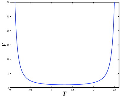
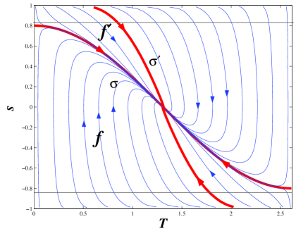
Figure 1: Potential and phase portrait for $k<0$ (here $k=-0.36$). The horizontal lines $s=\pm\sqrt{2/3}$ separate the central region where the expansion of the universe is accelerated from the two external regions where it decelerates.

The set of integral curves of (55) is symmetric under reflection with respect to the critical point (60): any given integral curve and its node (n)-reflected one describe the same cosmological evolution. The curve $\sigma$ corresponds to the eigenvalue $\lambda_{1}=-\frac{3}{2}\sqrt{\Lambda}(1+k)$, whose absolute value is the smallest of the two. It acts as a separatrix for the integral curves. Almost all curves approaching the node (60) end up there with the same tangent as $\sigma$. The only exception is a second separatrix $\sigma^{\prime}$ which corresponds to the eigenvalue $\lambda_{2}=-\frac{3}{2}\sqrt{\Lambda}(1-k)$. The curve $\sigma^{\prime}$ separates the bundle $f^{\prime}$ of the curves which do not intersect the axis $s=0$ from the bundle $f$ of those which intersect it (see Fig. 1). The boundary of the rectangle defined by Eqs. (58) and (59) describes a cosmological singularity. Indeed, the scalar curvature for a flat Friedmann universe is

$$R=6(\dot{h}+2h^{2}).$$ (63)

Since from Eqs. (1), (2), (4) and (5) one has that

$$\dot{h}=-\frac{3}{2}h^{2}s^{2}$$ (64)

by substituting into (63) it follows that

$$R=3h^{2}(4-3s^{2})=\frac{3V(T)(4-3s^{2})}{\sqrt{1-s^{2}}}.$$ (65)

Thus the scalar curvature $R$ tends to infinity when approaching the boundary of the rectangle (with the exception of the corners, that will be treated separately).

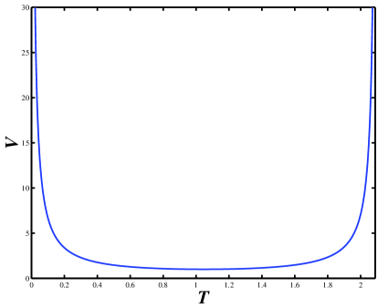
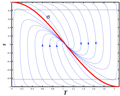
Figure 2: Potential and phase portrait for $k=0$. Since $k>-1/3$ there are trajectories which undergo two epochs of deceleration and two epochs of acceleration.

All integral curves end up in the node; let us see how they behave close to the boundary and begin with a right neighborhood of $T=0$. There equation (55) takes the form

$$\frac{ds}{dT}\approx\frac{2(1-s^{2})}{s\,T}\left(1-\frac{(-k)^{1/4}s}{\sqrt{1+k}(1-s^{2})^{1/4}}\right)=\frac{F(s)}{T}.$$ (66)

If $s<\sqrt{1+k}$, then $\dot{s}\rightarrow+\infty$ as $T\rightarrow 0$. Therefore, the integral curves at $s<\sqrt{1+k}$ which get close to the $T=0$ axis rise almost vertically, climbing leftwards for $s<0$ and rightwards for $s>0$ until they get close to $\sigma$ whenceforth they reach a maximum and thereafter approach the de Sitter node (60) (see Fig. 1). These are the curves of bundle $f$. If $\sqrt{1+k}<s<1$, then $\dot{s}\rightarrow-\infty$ as $T\rightarrow 0$. Therefore, the corresponding curves at $s>\sqrt{1+k}$ which get close to the $T=0$ axis drop almost vertically until they get close to $\sigma$ whenceforth they also approach the de Sitter node. These are the curves of bundle $f^{\prime}$. On the separatrix $\sigma$ one attains the point $(0,\sqrt{1+k})$ where $\dot{s}=0$. Symmetric considerations apply to the n-reflected curves, i.e. those which lie to the right of the separatrix $\sigma^{\prime}$.

But where do all the curves originate from? We first show that apart from $\sigma$, none of them can touch any point of the $s$-axis. Indeed, let us consider a point $(T,s)$ close to the $s$-axis. Eq. (66) can be integrated backwards to give

$$T(s)=T_{0}(s_{0})\exp\int_{s_{0}}^{s}\frac{dx}{F(x)}.$$ (67)

This equation shows that, if $F(s_{0})\not=0$, it is impossible to realize the condition $T_{0}(s_{0})=0$ and therefore touch the $s=0$ axis on a given trajectory. The roots of the equation $F(s_{0})=0$ are $s=\sqrt{1+k},\pm 1$. A closely similar reasoning excludes the point $(0,1)$. The point $(0,-1)$ can also be excluded since we should have $\dot{T}\geq 0$ in a neighborhood of such point; but $s$ is negative and this contradicts the equation $\dot{T}=s$. We are therefore left with the point $(0,\sqrt{1+k})$, where the exact solution $\sigma$ originates.

Let us examine now the upper boundary of Fig. 1. In a small neighborhood of the point $(T_{*},1)$ (where $T_{*}$ is in the domain (58)) Eq. (55) can be replaced by the following approximate equation:

$$\frac{d{s}}{dT}=-\frac{3(2(1-{s}))^{3/4}\sqrt{\Lambda}\left(1-(1+k)\cos^{2}\frac{3\sqrt{\Lambda(1+k)}T_{*}}{2}\right)^{1/4}}{\sin\frac{3\sqrt{\Lambda(1+k)}T_{*}}{2}}.$$ (68)

This equation is not Lipschtzian. The upper integral is the trivial solution $s=1$ while the lower integral is

$$s\rightarrow\left\{\begin{array}[]{lll}=1&{\rm for}&T<T_{*}\\ \thickapprox 1-C(T_{*})(T-T_{*})^{4}&{\rm for}&T\geq T_{*}\end{array}\right.$$ (69)

where

$$C(T_{*})=\frac{81}{32}\frac{\Lambda^{2}\left(1-(1+k)\cos^{2}\frac{3\sqrt{\Lambda(1+k)}T_{*}}{2}\right)}{\sin^{4}\frac{3\sqrt{\Lambda(1+k)}T_{*}}{2}}.$$ (70)

The intermediate solutions stay constant at $s=1$ for a while and then leave the $s=1$ line at a value $T_{**}>T_{*}$. Therefore, from each point $(T_{*},1)$ there originates only one integral curve behaving as (69). In particular, the separatrix $\sigma^{\prime}$ originates at a point $(T_{\sigma^{\prime}},1)$ (the value of $T_{\sigma^{\prime}}$ being unknown).

The condition of cosmic acceleration is

$$\frac{2\ddot{a}}{a}=-(\varepsilon+3p)>0.$$ (71)

For the tachyon cosmological model, using formulas (4) and (5) this condition can be reexpressed as

$$s^{2}<\frac{2}{3}.$$ (72)

Therefore, if $k\leq-\frac{1}{3}$ all cosmological evolutions undergo an initial phase of deceleration followed by an accelerating one. On the other hand, if $k>-\frac{1}{3}$ all evolutions whose originating point $T_{*}$ is larger than a critical value (which depends on $k$) have two epochs of deceleration and two epochs of acceleration. This happens in particular in the limiting case when $k=0$, as shown in Fig. 2.

We consider now the case $0<k<1$. Eq. (31) shows that the potential $V(T)$ is well defined only in the interval $(T_{3},T_{4})$ where

$$T_{3}=\frac{2}{3\sqrt{(1+k)\Lambda}}\arccos\frac{1}{\sqrt{1+k}},\ \ \ \ \ T_{4}=\frac{2}{3\sqrt{(1+k)\Lambda}}\left(\pi-\arccos\frac{1}{\sqrt{1+k}}\right).$$ (73)

Together with the condition $-1<s<1$, Eq. (73) defines the rectangle where we study the model at first. There are now three fixed points. One of them is the attractive de Sitter node (60) whereas the other two are saddles corresponding to the maxima of the potential at coordinates

$$T_{1}=\frac{2}{3\sqrt{(1+k)\Lambda}}\arccos\sqrt{\frac{1-k}{1+k}},\;\;\;\;\;T_{2}=\frac{2}{3\sqrt{(1+k)\Lambda}}\left(\pi-\arccos\sqrt{\frac{1-k}{1+k}}\right).$$ (74)

(s=0). They give rise to an unstable de Sitter regime with Hubble parameter

$$H_{1}=\sqrt{\frac{(1+k)\Lambda}{2\sqrt{k}}}>H_{0}.$$ (75)

We first analyze the behavior of the trajectories in the vicinity of the line $T=T_{3}$ and set $T=T_{3}+\tilde{T}$, with $\tilde{T}$ small and positive and $s\neq\pm 1$. With these conditions the model is described by the approximate equation

$$\dot{s}\approx-\frac{1-s^{2}}{2\tilde{T}},$$ (76)

which implies that the trajectories passing close to the boundary $T=T_{3}$ drop steeply down without crossing it. The ”physical” reason for this behavior is the vanishing of the potential at $T=T_{3}$ (to our knowledge this is a novel feature of our model); indeed, the structure of the tachyonic action implies that the ”force” is proportional to the logarithmic derivative of the potential and this is infinite at $T=T_{3}$. The impossibility of crossing $T=T_{3}$ remains true also without coupling the tachyon to gravity. On the other hand, in contrast with the situation encountered before, the geometry is regular at $T=T_{3}$: the vertical boundaries of the rectangle are not curvature singularities, because the potential does not diverge there. Actually, the curvature scalar $R$ vanishes there because of the vanishing of the potential.

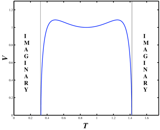
Figure 3: Potential for $k>0$ (here $k=0.44$).

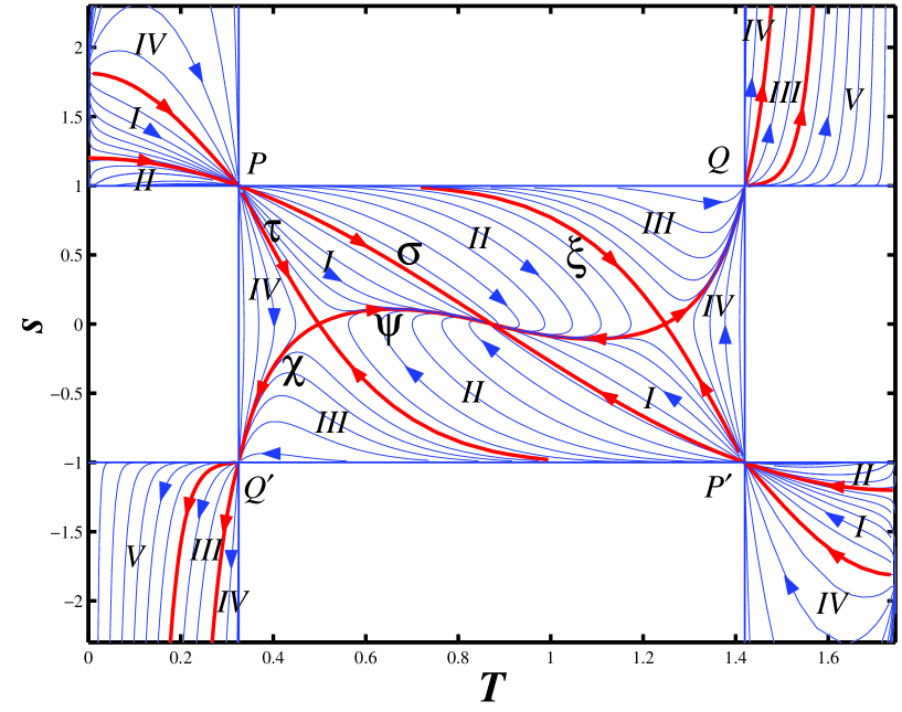
Figure 4: Phase portrait evolution for $k>0$ ($k=0.44$).

Instead, the horizontal sides are still singular. The situation is exactly as before and there is one integral curve which originates at $(T_{*},1)$ whose behavior is again given by (69), (70). Now, however, due to the positivity of the parameter $k$, the nonnegative function $C_{k}(T_{*})$ vanishes at $T=T_{3}$ and at $T=T_{4}$, is maximal at $T=T_{1}$ and at $T=T_{2}$, and has a positive local minimum at $T=T_{0}$.

Now consider the behavior of the trajectories in the upper left vertex of the rectangle $P=(T_{3},1)$. Setting $s=1-\tilde{s}$ and $T=T_{3}+\tilde{T}$, with $\tilde{T}$ and $\tilde{s}$ small but not zero, from Eq. (55) we get the approximate equation

$$\frac{d\tilde{s}}{d\tilde{T}}-\frac{\tilde{s}}{\tilde{T}}=A\,\tilde{s}^{3/4}\tilde{T}^{1/4},$$ (77)

where $A=3^{5/4}2^{3/4}\Lambda^{5/8}(1+k)^{5/8}k^{-3/8}.$ The general solution is

$$\tilde{s}=\frac{1}{256}(A\tilde{T}+B)^{4}\tilde{T},$$ (78)

where $B$ is an arbitrary constant. When $B\neq 0$ the leading behavior is

$$\tilde{s}=D\tilde{T},\,\,D>0.$$ (79)

This means that there are trajectories which gush out from the point $P$ in all possible directions, except of course vertically (see Fig. 4). If $B=0$ Eq. (78) becomes

$$\tilde{s}=\frac{A^{4}}{256}\tilde{T}^{5}.$$ (80)

This equation describes the leading behavior of a curve $\rho$ which separates the trajectories of type (79) from those originating at the points $(T_{*},1)$. We point out that $P$ is a cosmological singularity for the curve $\rho$ (which therefore originates at $P$), whereas it is regular for the curves (79). Indeed, we see from Eq. (1) that when $\tilde{T}\rightarrow 0\ \ h^{2}$ behaves as $1/\tilde{T}^{2}$ along $\rho$, while it is finite along trajectories (79).

Now consider the upper right vertex $Q=(T_{4},1)$. By setting as before $s=1-\tilde{s}$ and $T=T_{4}-\tilde{T}$ we get the approximate equation

$$\frac{d\tilde{s}}{d\tilde{T}}-\frac{\tilde{s}}{\tilde{T}}=-A\tilde{s}^{3/4}\tilde{T}^{1/4},$$ (81)

where $A$ is the same as above. The general solution is

$$\tilde{s}=\frac{1}{256}(-A\tilde{T}+B)^{4}\tilde{T},$$ (82)

where $B$ is an arbitrary positive constant. Therefore the trajectories enter point $Q$ along all possible directions except vertically and horizontally. We now classify the behavior of the trajectories in the interior of the rectangle. First note that there are five distinguished trajectories (separatrices): $\sigma$ which connects $P$ with the node; $\tau$ which connects $P$ with the saddle $(T_{1},0)$; $\xi$, which is the curve which enters the saddle $(T_{2},0)$ from above (We are unable to say whether $\xi$ originates at some point $(T_{*},1)$ or it belongs to the family (79), or it coincides with the curve $\rho$ defined by equation (80): for this reason we have not tried to draw curve $\rho$ in Fig 4); $\psi$, which originates from the saddle $(T_{1},0)$ and enters the node with tangent defined by the eigenvalue $\lambda_{2}=-\frac{3}{2}\sqrt{\Lambda}(1-k)$ (see (61)); finally, $\chi$ which connects $(T_{2},0)$ with $Q$ (see Fig. 4). Each of these separatrices has its own n-reflected counterpart (denoted by the same symbol).

Corresponding to the separatrices $\sigma,\tau,\xi,\psi$ and $\chi$ one can distinguish four bundles of qualitatively different trajectories. 1) The bundle $f^{I}$ of trajectories limited by $\tau,\psi$ and $\sigma$: they originate from $P$ and enter the node along $\psi$ and from above: 2) the bundle $f^{II}$ of trajectories limited by $\sigma,\xi$ and $\psi$ : they enter the node along $\psi$ from below; 3) the bundle $f^{III}$ of trajectories limited by $\xi,\chi$ and the horizontal line $s=1$; they stream into $Q$; 4) the bundle $f^{IV}$ of the curves which are limited by $\tau,\chi$ and the vertical line $T=T_{3}$: they gush out of $P$ and stream into $Q^{\prime}$.

Now we have to face a problem that we have not mentioned so far. The question is the following: it takes a finite proper time for the fields (and the universe) to get from anywhere to the corner $Q$ or $Q^{\prime}$ on a trajectory of bundle $f^{III}$ or of bundle $f^{IV}$. But these corners are not critical points of the dynamical system and, furthermore, the universe does not experience any singularity by getting there along these trajectories. Similar remarks apply to the past of the trajectories originating from $P$ and $P^{\prime}$. If the model could not be extended to follow these trajectories outside the rectangle where it has been originally defined it would be useless. However, we now show that this extension is actually possible. Indeed, one can see by inspection that the field equations are well defined also inside the four semi-infinite strips defined by the following inequalities: $0<T<T_{3}$, with $s>1$ or $s<-1$; $T_{4}<T<\frac{2\pi}{3\sqrt{\Lambda(1+k)}}$ with $s>1$ or $s<-1$. Then, following the strategy sketched in Section IV, we introduce a ”new” Lagrangian:

$$L=W(T)\sqrt{\dot{T}^{2}-1},$$ (83)

where the ”new” potential is given by

$$W(T)=\Lambda\frac{\sqrt{(k+1)\cos^{2}\frac{3\sqrt{\Lambda(1+k)}T}{2}-1}}{\sin^{2}\frac{3\sqrt{\Lambda(1+k)}T}{2}}.$$ (84)

The ”new” Lagrangian comes itself out of Sen’s action (Eqs. (3),(31)) by the previous trick:

$$V(T)\longrightarrow W(T)=iV(T)$$ (85)

$$\sqrt{1-\dot{T}^{2}}\longrightarrow i\sqrt{1-\dot{T}^{2}}=\sqrt{\dot{T}^{2}-1}$$ (86)

i.e. both the ”old” kinetic term and the potential become imaginary but their product remains real. It follows from the dynamics (55) that the expressions under the square root in the potential and the kinetic term change sign simultaneously. In other words, in the phase diagram no trajectory can cross any side of the rectangle. Thus, all the quantities characterizing the model keep real during the dynamical evolution. White regions in the phase diagram, where the Lagrangian and other quantities would become imaginary, are forbidden! The product (83), which amounts exactly to the ”old” Lagrangian, can be interpreted in terms of the ”new” kinetic term and potential that are both real. This makes it clear why the ”new” Lagrangian gives rise to field equations in the above four strips, which are the same as in the interior of the rectangle. At first glance one might have the impression that there is a freedom of choice of sign for the new Lagrangian (83), or, in other words, that one may choose opposite signs in Eqs. (86), (86). However, this is not so: the choice of sign in Eq. (83) is determined by the requirement of continuity of the Einstein (Friedmann) equations when passing from the rectangle to the stripes. As anticipated in Sec. IV, both the energy density and the pressure are positive in the considered strips.

However, there is an important difference between the present situation and the one described in Sec. IV. Here we are dealing with one single model ($k$ is fixed). One is compelled to make the extension of the model and, contrary to the $\Lambda=0$ case, the two different ”phases” (i.e. negative and positive pressure) are found within the same model, at different stages of the cosmic evolution, one phase in the rectangle, the other in the strips. In the following we give the precise mathematical meaning of this extension. This opens the way to the study of a new class of tachyon field theories.

We start by describing the behavior of the trajectories in the lower left strip (see Fig. 4). Since $\dot{T}<-1$, the evolution along any given trajectory will lead us in a finite amount of time to either hit the vertical line $T=0$ or to approach a vertical asymptote $T=T_{B}$, with $0\leq T_{B}<T_{3}$. The first alternative does not take place, whereas all values of $T_{B}$ in the indicated range are allowed, with the exception of $T_{B}=0$. Indeed, in the vicinity of $T=0$ Eq. (55) takes the following form

$$\frac{ds}{dT}=\frac{2(s^{2}-1)^{3/4}k^{1/4}}{\sqrt{1+k}\,T}-\frac{2(s^{2}-1)}{sT}.$$ (87)

Now, assume there is an $s_{0}<-1$ such that $\lim_{T\rightarrow 0}s(T)=s_{0}$. Then, the analogue of Eq. (67) gives a contradiction: the function $F(s)$ cannot vanish since the r.h.s. of Eq. (87) is positive.

The leading behavior of the solutions of Eq. (87) for $T\rightarrow 0$, $s\rightarrow-\infty$, is given by

$$|s|^{1/2}\approx\frac{1}{\frac{k^{1/4}}{\sqrt{1+k}}\ln\left(\frac{T}{T_{B}}\right)}$$ (88)

where $T_{B}$ is an arbitrary positive constant. It follows that the line $T=0$ is not an asymptote for any trajectory but of course there are trajectories whose asymptote is as close as we like to the line $T=0$.

Therefore, the trajectories inside the considered strip can be parameterized by the value $T_{B}$ of the coordinate of their vertical asymptote. We now discuss how they behave in the neighborhood of $s=-1$. As before we can divide the trajectories inside the strip into three families according to their leading behavior

$$s\approx-1+E(T-T_{3}),\ E>0,$$ (89)

$$s\approx-1+\frac{A^{4}}{256}(T-T_{3})^{5},$$ (90)

$$s\approx-1+C(T_{*})(T-T_{*})^{4},\ 0<T_{*}<T_{3}$$ (91)

Trajectories of type (89) fan out from point $Q^{\prime}$ into the strip at all possible angles. Trajectories of type (91) can be thought of as originating from $(T_{*},-1)$. Note that, just as before, the function $C(T_{*})$ approaches (minus) infinity as $T_{*}\rightarrow 0$. It approaches zero as $T_{*}\rightarrow T_{3}$. Curve (90) separates the families (89) and (91). The coordinate $T_{B}$ of the asymptote is an increasing function of $T_{*}$. As $T_{*}\rightarrow T_{3}$ it attains a value characterizing the asymptote of curve (90), beyond which it becomes an increasing function of $E$.

Let us go back to physics and consider the behavior of the cosmological radius $a(t)$ when the tachyon field $T(t)$ tends to $T_{B}$ along the solution of the field equations. The Friedmann equation implies that $h^{2}\rightarrow 0$ and that $\dot{h}\to-\infty$ (see Eq. (64)). Therefore, the scalar curvature (63) diverges and the universe reaches a cosmological singularity in a finite time.

This is an unusual type of singularity which we call big brake. Indeed, since ${\ddot{a}}/{a}=\dot{h}+h^{2}$, in a big brake we have that

$$\ddot{a}\rightarrow-\infty,$$

$$\dot{a}\rightarrow 0,$$

$$a\rightarrow a_{B}<\infty$$ (92)

In other words, the evolution of the universe comes to a screeching halt in a finite amount of time and its ultimate scale depends on the final value $T_{B}$ of the tachyon field.

We now turn to the behavior of the trajectories in the upper left strip. In the vicinity of $T=0$ the equation for the trajectories takes the form (87). The coefficient of ${T}^{-1}$ vanishes at the values

$$s=1,\ \sqrt{1+k},\ \sqrt{1+\frac{1}{k}}.$$ (93)

As explained earlier it is only at these values of $s$ that the trajectories can leave the line $T=0$. In addition, an analysis similar to the one performed earlier shows that the only trajectory starting at $(0,1)$ is the line $s=1$, and that the only trajectory starting at $(0,\sqrt{1+k})$ is the curve $\sigma$. All other trajectories start from $\left(0,\sqrt{1+\frac{1}{k}}\right)$. Eq. (87) shows that as $T\rightarrow 0$ the derivative $\frac{ds}{dT}$ approaches $-\infty$ for $\sqrt{1+k}<s<\sqrt{\frac{1+k}{k}}$ whereas it approaches $+\infty$ for $1<s<\sqrt{1+k}$ and $s>\sqrt{\frac{1+k}{k}}$ (see Fig. 4). To study the behavior in the neighborhood of $\left(0,\sqrt{\frac{1+k}{k}}\right)$ we set $s=\sqrt{\frac{1+k}{k}}+\tilde{s}$ with $\tilde{s}$ small. In the approximate equation for $\tilde{s}(T)$ it is necessary, besides the leading term , to keep the term proportional to $T$. Thus we get

$$\frac{d\tilde{s}}{dT}=\frac{2(1-k)}{1+k}\frac{\tilde{s}}{T}-\frac{9\Lambda}{8}\sqrt{\frac{1+k}{k}}\left(\frac{k+3}{k}\right)T.$$ (94)

The general solution of this equation is

$$\tilde{s}=\left(D-\frac{9\Lambda(1+k)^{3/2}(k+3)}{32k^{5/2}}T^{\frac{4k}{1+k}}\right)T^{\frac{2(1-k)}{1+k}},$$ (95)

where $D$ is an arbitrary constant. If $D\not=0$ we have the leading behavior

$${s}\approx\sqrt{1+\frac{1}{k}}+DT^{\frac{2(1-k)}{1+k}}$$ (96)

Therefore, if $k<\frac{1}{3}$ the trajectories start from $\left(0,\sqrt{1+\frac{1}{k}}\right)$ with horizontal tangent, whereas they start with vertical tangent when $k>\frac{1}{3}$. If $k=\frac{1}{3}$ they are born with any possible tangent. When $D=0$ we must go to the next order:

$${s}\approx\sqrt{1+\frac{1}{k}}-\frac{9\Lambda(1+k)^{3/2}(k+3)}{32k^{5/2}}T^{2}.$$ (97)

This curve acts as a separatrix for the curves having positive and negative $D$ respectively. Regarding the curves of the strip which lie below $\sigma$ they depart from $(T_{*},1)$ and behave in the neighborhood of this point as

$$s=1-C(T_{*})(T-T_{*})^{4},\ 0<T_{*}<T_{3},$$ (98)

where the function $C(T_{*})$ is the same as in (91). Regarding the behavior of the trajectories in the neighborhood of $T=T_{3}$ a simple analysis shows that they stream into $P$ at all possible angles (except vertically and horizontally). These properties show that each curve of type (96) with positive $D$ attains a maximum somewhere between $T=0$ and $T=T_{3}$ whose height is an increasing function of $D$ which tends to infinity as $D\rightarrow+\infty$.

So far, we have analyzed the behavior of the trajectories in two distinct regions: the rectangle and the four strips. Now, it has to be noted that the trajectories in the rectangle which leave $P$ (or $P^{\prime}$) at all possible angles in the open interval $(0,\pi/2)$ and the trajectories which enter $Q^{\prime}$ (or $Q$), again at all possible angles, are incomplete, since the vertices of the rectangle are not cosmological singularities for these curves. The same is true for the trajectories in the strips which enter $P$ (or $P^{\prime}$) and leave $Q$ (or $Q^{\prime}$). This circumstance, and the fact that the equation of motion for $T$ is the same in the rectangle and in the strips, indicates that it must be possible to extend and complete the above set of trajectories by continuation through the vertices of the rectangle. Precisely, the trajectories entering $P$ (or $P^{\prime}$) from the upper left (or lower right) strip shall be continued into the trajectories entering into the rectangle from $P$ (or $P^{\prime}$). Similar remarks apply to the corners $Q$ and $Q^{\prime}$. The uniqueness of this continuation procedure can be proved by applying the $\sigma$-process method of resolution of singularities (see, e.g. Arnold ). This amounts to blowing up (unfolding) the vertices of the rectangle by transition to suitable projective coordinates, the use of which removes the degeneracy of the vector field at these points. We do not give the mathematical details.

VI Cosmology

The rich mathematical structure that we have exhibited in the previous section gives rise to the possibility that cosmologies that have very different features coexist within the same model. In this sense tachyonic models are richer than the ”corresponding” standard scalar field models.

We now characterize all the evolutions in our model that are portrayed in Fig. 4. We start from the trajectories originating from the cosmological singularity $\left(0,\sqrt{1+\frac{1}{k}}\right)$ and which are characterized in the neighborhood of the latter by formula (96) with the parameter $D$ positive and very large. One such trajectory, as soon as it leaves the singularity, raises steeply upwards until it attains some maximum value. Henceforth it turns steeply downwards, enters the rectangle at $P$ at some small angle $\alpha$ with the vertical axis $T=T_{3}$ and moves towards $Q^{\prime}$. Upon reaching this point it enters the lower left strip and eventually ends up in a finite time $t_{B}$ in a big brake corresponding to some field value $T_{B}$ very close to $T_{3}$ (inf $t_{B}=0)$.

As $D$ decreases the height of the maximum decreases accordingly, $\alpha$ and $t_{B}$ increase and $T_{B}$ decreases. Eventually, at some critical value $D_{c}$ of the parameter $D$, the trajectory degenerates inside the rectangle with the separatrices $\tau$ and $\chi$ entering and, respectively, leaving the saddle point $(T_{1},0)$. The curves for which $D>D_{c}$ belong to the bundle $f^{IV}$. For $D<D_{c}$ we get the bundle $f^{I}$. These trajectories correspond to evolutions which are asymptotically de Sitter with a Hubble parameter $H_{0}=\sqrt{\Lambda}$. The upper bound of $D$ for the curves of bundle $f^{I}$ is $D_{c}$ and corresponds to the separatrix $\tau$ and $\psi$. This means that a tiny difference in the initial conditions will end up into dramatically different evolutions: one universe goes into an accelerating expansion of the de Sitter type and the other ends with a big brake. This should not be confused with a chaotic behavior: the two evolutions are almost indistinguishable for a very long time and then suddenly diverge from each other. As $D$ approaches $-\infty$ we end up into the separatrix $\sigma$ originating at the cosmological singularity $(0,\sqrt{1+k})$.

Proceeding further we encounter those evolutions which start at $(T_{*},1)$, $T_{*}<T_{3}$. In the neighborhood of the starting point they behave according to Eq. (98), then enter the rectangle through $P$ passing above the curve $\sigma$ from below. In the limit $T_{*}=T_{3}$ we obtain the trajectory $\rho$. As $T_{*}$ increases further beyond $T_{3}$ the curves detach themselves from the axis $s=1$ according to the equation (98) now with $T_{3}<T_{*}<T_{4}$. At some critical value $T_{*}^{c}$ of $T_{*},0<T_{*}^{c}<T_{4}$, the trajectory degenerates into the separatrices $\xi,\psi$ and $\chi$. The curves for which $0<T_{*}<T_{*}^{c}$ form the family $f^{II}$ and they asymptotically arrive at the de Sitter node $(T_{0},0)$ from below the axis $s=0$. Those for which $T_{*}^{c}<T_{*}<T_{4}$ form the family $f^{III}$; they enter the upper right strip through $Q$ and eventually end up in a finite time in a big brake. Finally, the trajectories that detach themselves from the axis $s=1$ at $T_{*}\geq T_{4}$ bend again upwards and they form another bundle that we denote by $f^{V}$. They also end up in a big brake.

The evolutions corresponding to the trajectories of the different bundles can also be studied in terms of the qualitative behavior of the Hubble parameter $h(t)$ as a function of time (see Fig. 5). In our model, using equations (1), (31) and (84) we get

$$h(t)=\frac{\sqrt{\Lambda}}{\sin\left(\frac{3\sqrt{\Lambda(1+k)}}{2}T(t)\right)}\left|\frac{1-(1+k)\cos^{2}\left(\frac{3\sqrt{\Lambda(1+k)}}{2}T(t)\right)}{1-s^{2}(t)}\right|^{\frac{1}{4}}.$$ (99)

Figure 5: Time evolution of the Hubble parameter $h(t)$.

Since $\dot{h}=-\frac{3}{2}h^{2}s^{2},\;$ $h(t)$ is positive and strictly decreasing, except at those values of $t$ for which $s(t)=0$.

Close to the initial singularity, the trajectories can be divided into two classes depending on the singular point from which each of them starts: the class (A) of trajectories originating at the point $(0,\sqrt{(1+k)/k})$ and the class (B) of trajectories which start from the points $(T_{*},1)$. The two classes are separated by the curve $\sigma$. The leading behavior of $h(t)$ in the neighborhood of the singularity at $t=0$ for the trajectories of class (A) is:

$$h(t)=\frac{2k}{3(1+k)}\frac{1}{t}-\frac{Dk}{3}\left(\frac{1+k}{k}\right)^{\frac{1-3k}{2(1+k)}}t^{\frac{1-3k}{1+k}}+\ldots,\;\;\;\;\; {\rm for\ \ }D\not=0;$$ (100)

$$h(t)=\frac{2k}{3(1+k)}\frac{1}{t}-\frac{k^{2}-2k+9}{32k}\Lambda t+\ldots,\;\;\;\;\; {\rm for\ \ }D=0.$$ (101)

For trajectories of class (B) the leading behavior is universal (it does not depend on $k$):

$$h(t)=\frac{2}{3t}+\ldots$$ (102)

To study the behavior of $h(t)$ at later times, one needs to examine each bundle $f$ separately, which, in turn, requires first plotting $h(t)$ for the different separatrices $\sigma,\tau,\xi,\psi$ and $\chi$.

We have from Eq. (57) that $h(t)$ for the separatrix $\sigma$ is given by

$$h_{\sigma}(t)=\sqrt{\Lambda}\coth\left(\frac{3\sqrt{\Lambda}(1+k)t}{2}\right)$$ (103)

In particular, in the neighborhood of $t=0$,

$$h_{\sigma}(t)=\frac{2}{3(1+k)}\frac{1}{t}+\frac{\Lambda(1+k)}{2}t+\ldots$$ (104)

to be compared with Eqs. (100), (101) and (102). Furthermore, $h_{\sigma}(t)$ is strictly decreasing and, as $t\to\infty$, it approaches a stable de Sitter expansion with Hubble parameter $\sqrt{\Lambda}$.

Regarding the unstable cosmological evolution $h_{\tau}(t)$, for small $t$ we have

$$h_{\tau}(t)=\frac{2k}{3(1+k)}\frac{1}{t}-\frac{D_{c}k}{3}\left(\frac{1+k}{k}\right)^{\frac{1-3k}{2(1+k)}}t^{\frac{1-3k}{1+k}}+\ldots$$ (105)

and $\lim_{t\to\infty}h_{\tau}(t)=H_{1}$ (see Fig. 5 and Eq. (75)). Qualitatively, $h_{\tau}(t)$ behaves similarly to $h_{\sigma}(t)$ but the asymptotic value of the Hubble parameter is higher. As for the separatrix $\psi$, the corresponding cosmological evolution is unstable and non singular: the Hubble parameter decreases steadily from an unstable de Sitter regime $h_{\psi}({-\infty})=H_{1}$ at large negative times to a stable one $h_{\psi}(\infty)=\sqrt{\Lambda}$ at large positive times. $h_{\xi}(t)$ and $h_{\tau}(t)$ have qualitatively similar behaviors at large times while they are different at small times. Finally, $h_{\chi}(t)$ decreases steadily from an unstable asymptotic de Sitter value $h_{\chi}({-\infty})=H_{1}$ at large negative times to the final big brake singularity $h_{\chi}(t_{B})=0$, with $\dot{h}_{\chi}(t_{B})=-\infty$, for some suitable $t_{B}$.

For a trajectory of bundle $f^{I}$ which lies close to the sepratrices $\tau$ and $\psi$, $h(t)$ behaves according to (100) close to the initial singularity, with $D<D_{c}$, $(D_{c}-D)$ small. Then $h(t)$ decreases steadily and remains close to $h_{\tau}(t)$ for a very long time during which $s$ (and hence $\dot{h}$) gets close to zero. Therefore, in this regime the evolution simulates an asymptotic de Sitter expansion with Hubble parameter close to the value $H_{1}$. Eventually, however, $s$ starts increasing again and the graph of $h(t)$ bends downwards away from $h_{\tau}(t)$ and approaches asymptotically the stable de Sitter regime with Hubble parameter $\sqrt{\Lambda}$. Instead, for a trajectory of bundle $f^{I}$ which lies very close $\sigma$ the behavior $(\ref{3.2})$ of $h(t)$ at small times is characterized by a value of the constant $D$ which is negative and very large; the graph of $h(t)$ parts only slightly from the graph of $h_{\sigma}(t)$ and the asymptotic value $\sqrt{\Lambda}$ is approached much earlier. Other elements of $f^{I}$ display behaviors which are intermediate between those described above. The time dependence of $h$ for the trajectories of bundle $f^{II}$ is qualitatively similar to the one relative to the curves of $f^{I}$, the differences being the following: the small time behavior is given by (102), and for each trajectory of $f^{II}$ there is a value $t_{0}$ of $t$ (which depends on the particular trajectory) for which $s(t_{0})=0$ so that $\dot{h}(t_{0})=0$.

Now consider a curve of bundle $f^{III}$ which lies very close to the separatrices $\xi$ and $\chi$. For such a curve $h(t)$ remains very close to $h_{\xi}(t)$ for a very long time, $s(t)$ decreases getting close to zero and the evolution simulates again an asymptotic de Sitter expansion with Hubble parameter. However, eventually $s(t)$ starts increasing indefinitely and in a finite (though long) time the cosmology end up in a big brake. Moving to curves that are farther and farther away from $\xi$ and $\chi$, the value $T_{*}$ of $T$ at the initial singularity moves to the right towards the value $2\pi/(3\sqrt{\Lambda(1+k)})$, $h(t)$ decreases more and more steeply and the big brake time $t_{B}$ tends to zero (when $T_{*}$ gets larger than $T_{4}$ the trajectories switch from bundle $f^{III}$ to bundle $f^{V}$).

Like those of bundles $f^{III}$ and $f^{V}$, the evolutions of bundle $f^{IV}$ give likewise rise to a big brake and the behavior of $h(t)$ is qualitatively similar in the two cases. However, contrary to what happens for bundles $f^{III}$ and $f^{V}$, for each trajectory of bundle $f^{IV}$ there is a time $t=t_{0}$ (which depends on the particular trajectory and spans the whole open half line) for which $s(t_{0})=0$ and hence $\dot{h}(t_{0})=0$. Therefore, even though the big brake time can get as close to zero as one likes for the curves of type $IV$ (for such curves, $t_{B}$ is a decreasing function of the parameter $D$ in Eq. (100), with $\lim_{D\to D_{c}}t_{B}(D)=\infty$ and $\lim_{D\to\infty}t_{B}(D)=0$) and hence $h(t)$ may decrease to zero very steeply, there is always some intermediate time at which $h(t)$ is momentarily stationary. Remark that, as one can see from Fig. 5, there is nothing peculiar in the behavior of $h(t)$ at the times when vertices of the rectangle are crossed.

The possibility of cosmological singularities characterized by the divergence of the second time derivative of the cosmological scale factor has also been considered in Sahni-brake in the brane cosmology context.

We conclude this section by another simple example of cosmology sharing this property. Let us consider the flat Friedmann universe filled with a perfect fluid with a state equation similar to (40):

$$p=\frac{A}{\varepsilon}$$ (106)

where $A$ is positive. We can call this fluid the ”anti-Chaplygin gas”. This equation of state arises in the study of the so-called wiggly strings Carter ; Vilenkin . The dependence of the energy density on the cosmological radius is given by

$$\varepsilon=\sqrt{\frac{B}{a^{6}}-A},$$ (107)

where $B$ is a positive constant. At the beginning of the cosmological evolution $\varepsilon\sim\sqrt{B}/a^{3}$, like in the dust-dominated case. Now there is a maximal value possible for the cosmological scale

$$a_{F}=\left(\frac{B}{A}\right)^{1/6}.$$ (108)

that is attained in a finite cosmic time $t_{F}$. The behavior of $a(t)$ in the vicinity of the maximum is the following

$$a(t)\thickapprox a_{F}-C(t_{F}-t)^{4/3},\;\;\;\;\ C=2^{-7/3}3^{5/3}(AB)^{1/6}.$$ (109)

Since $\dot{a}(t_{F})=0$ while $\ddot{a}(t_{F})=-\infty$ we are back into a big brake cosmological singularity.

Thus, a big brake singularity can be found in an elementary cosmological model (though based on an exotic fluid). The difference with the tachyonic model is that in the latter there are evolutions culminating in a big brake which co-exist with other evolutions giving rise to an infinite accelerated expansion. These two types of evolutions correspond to different classes of initial conditions.

It maybe worth mentioning that also for $k>0$ one can construct a scalar field model; indeed the potential displayed in Eq. (29) is not restricted to $k<0$. But this model has a much poorer dynamics: all the trajectories tend to the de Sitter attractive node point.

VII Final considerations: fate of the universe

The study of the fate or the future of the universe is rather popular nowadays Dyson –Sahni-bounce , and, as was predicted more than 20 years ago by F.J. Dyson Dyson , “eschatology” has now become part of the cosmological studies. This sort of studies include of course also biological aspects of and the fate of consciousness in the different cosmological scenarios (see, for example, Dyson ; Freese ; Bar-Tip ) but our goal is much more modest and we shall concentrate on the purely geometrical facet of the topic.

There are three mainly studied possible scenarios for the future of the universe, intensively discussed in literature: an infinite expansion; an expansion followed by a contraction ending in a “big crunch”; an infinitely bouncing or recycling universe.

The present set of observational data seems to favor the first scenario: the data are quite compatible with a flat universe with a positive cosmological constant.

On the other hand a negative value of the cosmological constant fits better with string theory (see, e.g. Gibbons ; Kal-Lin ; Kal-Lin1 ). The presence of a small negative cosmological constant could be made compatible with the present day cosmic acceleration, provided there are some fields or types of matter responsible for this acceleration. However, in this context the cosmological radius sooner or later will start decreasing and the expansion will be followed by a contraction which would normally lead the universe to a cosmological singularity of the big crunch type.

The third scenario of an infinitely bouncing or recycling universe appears to many to be very attractive because it opens an opportunity to escape the “frying” in the big crunch and the “freezing” in the infinite expansion case. In this scenario, during the process of contraction there will be two opportunities: collapse or bounce with subsequent expansion. The choice of one of these opportunities depends on the initial conditions and this dependence has usually a chaotic character Page ; KKT ; KKT1 ; Corn ; KKST .

Furthermore, one can show Kal-Lin1 that for every model of dark energy describing an eternally expanding universe one can construct many closely related models which describe the present stage of acceleration of the universe followed by its global collapse. However, these models corresponding to eternally expanding and collapsing universes are different and have different values of their basic parameters.

One interesting feature of our toy tachyon model is that the first and the second scenario coexist in its context. Depending on initial conditions, some correspond to eternal expansions of the universe which approach asymptotically a pure de Sitter regime, while others end their evolution at the cosmological singularity.

The second distinguishing feature of this model is that the singularity at which the universe ends its evolution is not a standard big crunch singularity. Instead, it corresponds to a finite non zero cosmological radius at which the Hubble parameter is finite and the deceleration parameter is infinite and has positive sign. We have called this fate ”big brake”. The prospect of hitting the cosmological singularity during expansion has been also discussed in Ref. Star-fut , where the singularity corresponds to an infinite value of the Hubble variable and the cosmological radius. This scenario is known as ”big rip” or ”phantom cosmology” (see, e.g. doomsday ; sami-phan ; marek ; sami-top ).

The third distinguishing aspect of our model is the fact that the regions of the phase space corresponding to different types of trajectories are well separated and the dependence of the cosmology on the choice of initial conditions is quite regular (non chaotic). A remark is in order here: the chaoticity of the classical dynamics hinders the application of the WKB approximation and, hence, undermines the basis of the majority of results of quantum cosmology Corn . In our model quantum- cosmological schemes of the traditional type Hartle-Hawk ; Hawk ; Vil ; Vil1 can be attempted. The corresponding wave function should describe a probability distribution over different initial conditions for the classical evolution of the universe. The quantum evolution of the universe in our toy model might be expressed in the language of the many-worlds interpretation of quantum mechanics Everett ; DeWitt . In this framework one can say that the wave function of the universe describes the quantum birth of the universe and subsequently the process of the so called “classicalization” (see e.g. Ref. Bar-Kam ). During this process the wave function splits into different branches or Everett worlds corresponding to different possible classical histories of the universe. The peculiarity of our toy model consists in the fact that some of these branches describe eternally expanding universes while other branches correspond to universes which end their evolution hitting the cosmological singularity.

References

- (1) A. Riess et al., Observational Evidence from Supernovae for an Accelerating Universe and a Cosmological Constant, Astron. J. 116 (1998) 1009; astro-ph/9805201.
- (2) S.J. Perlmutter et al., Measurements of Omega and Lambda from 42 High-redshift Supernovae, Astroph. J. 517 (1999) 565, astro-ph/9812133.
- (3) N.A. Bachall, J.P. Ostriker, S. Perlmutter and P.J. Steinhardt, The Cosmic Triangle: Revealing the State of the Universe, Science 284 (1999) 1481; astro-ph/9906463.
- (4) V. Sahni and A.A. Starobinsky, The Case for a Positive Cosmological Lambda-term, Int. J. Mod. Phys. D 9 (2000) 373 ; astro-ph/9904398.
- (5) T. Padmananbhan, Cosmological constant - the weight of the vacuum, Phys. Rep. 380 (2003) 235; hep-th/0212290.
- (6) A. Sen, Rolling Tachyon, JHEP 0204 (2002) 048; hep-th/0203211.
- (7) A. Sen, Tachyon Matter, JHEP 0207 (2002) 065; hep-th/0203265.
- (8) A. Sen, Field Theory of Tachyon Matter, Mod.Phys.Lett. A17 (2002) 1797; hep-th/0204143.
- (9) M.R. Garousi, Tachyon couplings on non-BPS D-branes and Dirac-Born-Infeld action, Nucl. Phys. B584 (2000) 284; hep-th/0003122.
- (10) G.W. Gibbons, Cosmological evolution of the rolling tachyon, Phys. Lett. B537 (2002) 1; hep-th/0204008.
- (11) M. Fairbairn and M.H.G. Tytgat, Inflation from a tachyon fluid?, Phys. Lett. B546 (2002) 1; hep-th/0204070.
- (12) S. Mukohyama, Brane cosmology driven by the rolling tachyon, Phys. Rev. D66 (2002) 024009, hep-th/0204084.
- (13) A. Feinstein, Power-Law Inflation from the Rolling Tachyon, Phys. Rev. D 66 (2002) 063511; hep-th/0204140.
- (14) T. Padmanabhan, Accelerated expansion of the universe driven by tachyonic matter, Phys. Rev. D 66 (2002) 021301; hep-th/0204150.
- (15) A. Frolov, L. Kofman and A. Starobinsky, Prospects and Problems of Tachyon Matter Cosmology, Phys. Lett. B545 (2002) 8; hep-th/0204187.
- (16) T. Padmanabhan and T. Roy Choudhury, Can the clustered dark matter and the smooth dark energy arise from the same scalar field?, Phys. Rev. D66 (2002) 081301; hep-th/0205055.
- (17) H.B. Benaoum, Accelerated Universe from modified Chaplygin gas and Tachyonic Fluid, hep-th/0205140.
- (18) M. Sami, Aspects of tachyonic inflation with exponential potential, Phys. Rev. D66 (2002) 043530; hep-th/0205179.
- (19) J.M. Cline, H. Firouzjahi and P. Martineau, Reheating from tachyon condensation, JHEP 0211 (2002) 041; hep-th/0207156.
- (20) G. N. Felder, L. Kofman, A. Starobinsky, Caustics in Tachyon Matter and Other Born-Infeld Scalars, JHEP 0209 (2002) 026; hep-th/0208019.
- (21) J.S. Bagla, H.K. Jassal and T. Padmanabhan, Cosmology with tachyon field as dark energy, Phys. Rev. D67 (2003) 063504; astro-ph/0112198.
- (22) G.W. Gibbons, Thoughts on Tachyon Cosmology, hep-th/0301117.
- (23) L.R.W. Abramo and F. Finelli, Cosmological dynamics of the tachyon with an inverse power-law potential, astro-ph/0307208.
- (24) M.-B. Causse, A rolling tachyon field for both dark energy and dark halos of galaxies, astro-ph/0312206.
- (25) B.C. Paul, A note on inflation with tachyon rolling on the Gauss-Bonnet brane, hep-th/0312081.
- (26) A. Sen, Remarks on tachyon driven cosmology, hep-th/0312153.
- (27) M.R. Garousi, M. Sami and S. Tsujikawa, Inflation and dark energy arising from rolling massive scalar field on the D brane, hep-th/0402075.
- (28) G. Calcagni, Slow roll parameters in braneworld cosmologies, hep-ph/0402126.
- (29) J.M. Aguirregabiria and R. Lazkoz, A note on the structural stability of tachyonic inflation, gr-qc/0402060.
- (30) J.M. Aguirregabiria and R. Lazkoz, Tracking solutions in tachyon cosmology, hep-th/0402190.
- (31) A.A. Starobinsky, How to determine an effective potential for a variable cosmological term, JETP Lett. 68 (1998) 757; astro-ph/9810431.
- (32) F. Lucchin and S. Matarrese, Power law inflation, Phys. Rev. D32 (1985) 1316.
- (33) J.J. Halliwell, Scalar fields in cosmology with an exponential potential, Phys. Lett. B185 (1987) 341.
- (34) J.D. Barrow, Cosmic no hair theorem and inflation, Phys. Lett. B 187 (1987) 12.
- (35) A.B. Burd and J.D. Barrow, Inflationary models with exponential potentials, Nucl. Phys. B 308 (1988) 929.
- (36) B. Ratra, Inflation in an exponential potential scalar field model, Phys. Rev. D45 (1992) 1913.
- (37) J.D. Barrow, Graduated inflationary universes, Phys. Lett. B 235 (1990) 40.
- (38) J. Lidsey, Multiple and anisotropic inflation with exponential potentials, Class. Quant. Grav.9 (1992) 1239.
- (39) S. Capozziello, R. de Ritis, C. Rubano and P. Scudellaro, Noether symmetries in cosmology, Riv. del Nuovo Cimento 19 (1996) 1.
- (40) A. A. Coley,J. Ibanez, R. J. van den Hoogen, Homogeneous scalar field cosmologies with an exponential potential, J. Math. Phys. 38 (1997) 5256.
- (41) C. Rubano and P. Scudellaro, On Some Exponential Potentials for a Cosmological Scalar Field as Quintessence, Gen. Rel. Grav.34 (2002) 307; astro-ph/0103335.
- (42) A.Yu. Kamenshchik, U. Moschella and V. Pasquier, An alternative to quintessence, Phys. Lett. B511 (2001) 265; gr-qc/0103004.
- (43) J.C. Fabris, S.V.B. Gonasalves and P.E. de Souza, Density perturbations in an Universe dominated by the Chaplygin gas, Gen. Rel. Grav. 34 (2002) 53; gr-qc/0103083.
- (44) N. Bilic, G.B. Tupper and R. Violler, Unification of Dark Matter and Dark Energy: the Inhomogeneous Chaplygin Gas, Phys. Lett. B535 (2002) 17; astro-ph/0111325.
- (45) M.C. Bento, O. Bertolami and A.A. Sen, Generalized Chaplygin Gas, Accelerated Expansion and Dark Energy-Matter Unification, Phys. Rev. D66 (2002) 043507; gr-qc/0202064.
- (46) V. Gorini, A.Yu. Kamenshchik and U. Moschella, Can the Chaplygin gas be a plausible model for dark energy?, Phys. Rev. D67 (2003) 063509; astro-ph/0209395.
- (47) P.P. Avelino, L.M.G. Beca, J.P.M. de Carvalho, C.J.A.P. Martins and P. Pinto, Alternatives to quintessence model-building, Phys. Rev. D67 (2003) 023511; astro-ph/0208528; M. Makler, S. Quinet de Oliveira and I. Waga, Constraints on the generlaized Chaplygin gas from supernovae observations, Phys. Lett. B 555 (2003) 1; astro-ph/0209486; J.S. Alcaniz, D. Jain and A. Dev, High-redshift objects and the generalized Chaplygin gas, Phys. Rev. D67 (2003) 043514; astro-ph/0210476; M.C. Bento, O. Bertolami and A.A. Sen Generalized Chaplygin gas and CMBR constaints, Phys. Rev. D67 (2003) 063003; astro-ph/0210468; R. Colistete, Jr., J.C. Fabris, S.V.B. Goncalves and P.E. de Souza, Bayesian analysis of the Chaplygin gas and cosmological consstant models using the SNE Ia data, astro-ph/0303338; L. Amendola, F. Finelli, C. Buriana and D. Carturan, WMAP and the generalized Chaplygin gas, JCAP 0307 (2003) 005; astro-ph/0304325; P.P. Avelino, L.M.G. Beca, J. P. M. de Carvalho and C.J.A.P. Martins, The Lambda CDM limit of the generalized Chaplygin gas scenario, JCAP 0309 (2003) 002; astro-ph/0307427; N. Bilic, R.J. Lindebaum, G.B. Tupper and R.D. Viollier, The Chaplygin gas and the evolution of dark matter and dark energy in the universe, astro-ph/0307214; J.S. Alcaniz and J.A.S. Lima, Measuring the Chaplygin gas equation of state from angular and luminosity distances, astro-ph/0308465.
- (48) V.I. Arnold, Geometrical methods in the theory of ordinary differential equations, Grundlehren,vol. 250, Springer, 1983.
- (49) Yu. Shtanov and V. Sahni, New Cosmological Singularities in Braneworld Models, Class.Quant.Grav. 19 (2002) L101; gr-qc/0204040.
- (50) B. Carter, Duality relation between charged elastic strings and superconducting cosmic strings, Phys. Lett. B224 (1989) 61.
- (51) A. Vilenkin, Effect of small scale structure on the dynamics of cosmic strings, Phys. Rev. D41 (1991) 3038.
- (52) F.J. Dyson, Time without end: Physics and biology in an open universe, Rev. Mod. Phys. 51 (1979) 447.
- (53) F.C. Adams and G. Laughlin, A dying universe: the long term fate and evolution of astrophysical objects, Rev. Mod. Phys. 69 (1997) 337, astro-ph/9701131.
- (54) G. Starkman, M. Trodden and T. Vachaspati, Observation of cosmic acceleration and determining the fate of the universe, Phys. Rev. Lett. 83 (1999) 1510; astro-ph/9901405.
- (55) L.M. Krauss and M.S. Turner, Geometry and Destiny, Gen. Rel. Grav.31 (1999) 1453; -1459;astro-ph/9904020.
- (56) M. Ozer, Fate of the universe, age of the universe, dark matter, and the decaying vacuum energy, Astrophys. J. 520 (1999) 45; astro-ph/9911246.
- (57) A.A. Starobinsky, Future and origin of our universe: modern view, Grav. Cosmol. 6 (2000) 157; in “The Future of the Universe and the Future of our Civilization”, eds. V. Burdyuzha and G. Khozin, World Scientific (Singapore), 2000, 71; astro-ph/9912054.
- (58) P.P. Avelino, J.P.M. de Carvalho and C.J.A.P. Martins, Can we predict the fate of the universe, Phys. Lett. B501 (2001) 257; astro-ph/0002153.
- (59) F.J. Tipler, The ultimate future of the Universe, black hole event horyzon Topologies, holography, and the value of the cosmological constant, in “Austin 2000, Relativistic astrophysics” 769; astro-ph/0104011.
- (60) D. Huterer, G.D. Starkman and M. Trodden, Is the universe inflating? Dark energy and the future of the universe, Phys. Rev. D66 (2002) 043511; astro-ph/0202256.
- (61) K. Freese and W. Kinney, The Ultimate Fate of Life in an Accelerating Universe, astro-ph/0205279.
- (62) R. Kallosh, A. Linde, S. Prokushkin and M. Shmakova, Supergravity, dark energy and the fate of the universe, Phys. Rev. D66 (2002) 123503; hep-th/0208156.
- (63) R. Kallosh and A. Linde, Dark energy and the fate of the universe, JCAP02(2003)002; astro-ph/0301087.
- (64) U. Alam, V. Sahni and A.A. Starobinsky, Is dark energy decaying?, JCAP04(2003)002; astro-ph/0302302.
- (65) R.R. Caldwell, M. Kamionkowski and N.N. Weinberg, Phantom energy: Dark energy with causes a cosmic doomsday, Phys. Rev. Lett. 91 (2003) 071301; astro-ph/0302506.
- (66) R. Kallosh, J. Kratochvil, A. Linde, E.V. Linder and M. Shmakova, Observational bounds on cosmic doomsday, astro-ph/0307185.
- (67) M. Sami, Cosmological dynamics of phantom field, Phys. Rev. D68 (2003) 023522; hep-th/0305110.
- (68) M. P. Dabrowski, T. Stachowiak and M. Szydlowski, Phantom cosmologies, hep-th/0307128.
- (69) M. Sami and A. Toporensky, Phantom field and the fate of the universe, gr-qc/031209.
- (70) S.W. Hawking, Quantum Cosmology, in “Relativity, Groups and Topology II”, North-Holland Physics Publ., Amsterdam, 1984, 333.
- (71) D.N. Page, A Fractal Set Of Perpetually Bouncing Universes? Class. Quant. Grav. 1 (1984) 417.
- (72) M.A. Markov, Probelms of a perpetually oscillating universe, Ann. Phys. (N.Y.) 155 (1984) 333.
- (73) R. Durrer and J. Laukenmann,The Oscillating Universe: an Alternative to Inflation, Class. Quant. Grav. 13 (1996) 1069; gr-qc/9510041.
- (74) A.Yu.Kamenshchik, I.M.Khalatnikov and A.V.Toporensky, Simplest cosmological model with the scalar field, Int. J. Mod. Phys. D 6 (1997) 673; gr-qc/9801064.
- (75) A.Yu.Kamenshchik, I.M.Khalatnikov and A.V.Toporensky, Simplest cosmological model with the scalar field II. Influence of cosmological constant, Int. J. Mod. Phys. D7 (1998) 129; gr-qc/9801082.
- (76) N.J. Cornish and E.P.S. Shellard, Chaos in quantum cosmology, Phys. Rev. Lett. 81 (1998) 3571; gr-qc/9708046.
- (77) A.Yu.Kamenshchik, I.M.Khalatnikov, S.V. Savchenko and A.V.Toporensky, Topological entropy for some isotropic cosmological models, Phys.Rev. D59 (1999) 123516; gr-qc/9809048.
- (78) N. Kanekar, V. Sahni and Yu. Shtanov, Recycling the universe using scalar fields, Phys. Rev. D63 (2001) 083520; astro-ph/0101448.
- (79) Yu. Shtanov and V. Sahni, Bouncing Braneworlds, gr-qc/0208047.
- (80) J.D. Barrow and F. Tipler, The Antropic Cosmological Principle, Oxford University Press, 1986.
- (81) J.B. Hartle and S.W. Hawking, Wave function of the universe, Phys. Rev. D28 (1983) 2960.
- (82) S.W. Hawking, The quantum state of the universe, Nucl. Phys. B239 (1984) 257.
- (83) A. Vilenkin, Quantum creation of universes, Phys. Rev. D30 (1984) 509.
- (84) A. Vilenkin, Quantum cosmology and the initial state of the universe, Phys. Rev. D37 (1988) 888.
- (85) H. Everett, Relative state formulation of quantum mechanics, Rev. Mod. Phys. 29 (1957) 454.
- (86) The Many Worlds Interpretation of Quantum Mechanics, Eds. B.S. DeWitt and R.N. Graham, Princeton University Press, Princeton, NJ, 1973.
- (87) A.O. Barvinsky and A.Yu. Kamenshchik, Preferred basis in quantum theory and the problem of classicalization of the quantum universes, Phys. Rev. D52 (1995) 743.