hep-th/0311095
HWS-2003A11
November 2003
Duality and Central Charges
in Supersymmetric Quantum Mechanics

We identify a class of point-particle models that exhibit a target-space duality. This duality arises from a construction based on supersymmetric quantum mechanics with a non-vanishing central charge. Motivated by analogies to string theory, we are led to speculate regarding mechanisms for restricting the background geometry.
PACS: 11.30.Pb , 11.25.Tq , 03.65-w

One phenomenon usually regarded as peculiarly “stringy” is that of space-time duality. The simplest instance occurs when a quantum string propagates in a ten-dimensional target space involving one compact circular spatial dimension having radius $R$. In this case, $T$-duality [1] exchanges quantized Kaluza-Klein momentum modes with wrapping modes of the string, and at the same time replaces $R\to\alpha^{\prime}/R$. Since wrapping modes are characteristic of extended objects, one might not expect to find a similar duality connecting ostensibly distinct point particle models with different classical background geometries. In this letter, we demonstrate that, surprisingly, a similar duality does hold for the case of a supersymmetric point particle propagating on a manifold with the topology of a cylinder, provided one incorporates a nontrivial central charge into the supersymmetry algebra. In this context, Kaluza-Klein modes are clearly present, and correspond to momenta of the particle directed around the cylinder. But the wrapping modes of the string are replaced with a central charge parameter whose physical origin is at present obscure.

Supersymmetric quantum mechanics [2] can be formulated as a one-dimensional supersymmetric quantum field theory; the lone dimension in this context is time. A bosonic field is, then, a real-valued function of time, and a fermionic field is a Grassman-valued function of time. The $d=1$, $N=1$ superalgebra with a central charge is specified by the following relations,

$$\{\,Q\,,\,Q^{\dagger}\,\}=2\,H\hskip 28.90755pt[\,H\,,\,Q\,]=0\hskip 28.90755ptQ^{2}=Z\,,$$ (1)

where $Q$ is the complex supercharge, $Z$ is the complex central charge, and $H$ is the Hamiltonian. A consequence of the super-Jacobi identity is that $Z$ and $Z^{\dagger}$ each commute with $Q$ and with $Q^{\dagger}$. Note that $[\,H\,,\,Q\,]=0$ must be specified as an independent condition when $Z\neq 0$.

In higher dimensional field theories, central charges can appear in superalgebras owing to topological features of solitonic background field configurations [3, 4]. In practice, these quantities arise as surface terms in integrals appearing in superalgebra anticommutators. When formulating quantum mechanics as a field theory, however, there are no spatial integrals to produce such boundary terms. Therefore, a topological explanation for the appearance of the central charge in (1) would require a suitably modified version of the usual field-theoretic explanation. One possibility in this regard would involve centrally-extended supersymmetric quantum mechanics as the natural description of effective physics localized on topological zero-branes present in higher dimensional field theories, such as a “kink” soliton in a two-dimensional WZW model which has degenerate classical vacua [5], or a point-like intersection of two one-dimensional domain walls in a three-dimensional WZW model [6, 7].

When a charge is topological in origin, it is naturally quantized. For this reason, the scenarios described above conceivably provide a rationale for the quantization of the central charge term in (1). In this paper, however, we view this charge simply as an allowable extension to the algebra, and investigate the ramifications. There is no a priori reason, from an algebraic perspective, that this charge should be quantized. Nevertheless, a duality we uncover in this paper suggests the existence of a more fundamental construction underlying the class of models we introduce, in which the central charge is quantized, perhaps in a manner similar to the examples described above.

In this letter, we restrict attention to the case that the central charge $Z$ is real. We do this for two reasons, which we believe may be related to each other. First, this restriction appears naturally when a two-dimensional (1,1) superalgebra is compactified to one dimension; in this case, the real central charge in the compactified algebra corresponds to the two-dimensional momentum component directed around the compactified dimension. Second, as we show in [8], the above superalgebra with real central charge supplies a natural setting for understanding the shape invariance approach to exact solubility [9, 10, 11, 12].

In terms of “pre-quantum” classical constructions, superalgebras are represented by transformation rules interrelating components of irreducible multiplets. A supersymmetry transformation is expressed as $\delta_{Q}(\epsilon)=\epsilon\,Q+\epsilon^{\dagger}\,Q^{\dagger}$, where $\epsilon$ is a complex Grassman parameter. In terms of this operation, the $N=1$ superalgebra can be written, in the case of a real central charge, as

$$[\,\delta_{Q}(\epsilon_{1})\,,\,\delta_{Q}(\epsilon_{2})\,]=-4\,i\,\epsilon_{[1}^{\dagger}\,\epsilon_{2]}\,\partial_{t}-2\,i\,(\,\epsilon_{1}\,\epsilon_{2}+\epsilon_{1}^{\dagger}\,\epsilon_{2}^{\dagger}\,)\,\delta_{Z}\,,$$ (2)

where we have used the canonical representation of the Hamiltonian as the generator of time translations, $H=i\,\partial_{t}$, and have defined a “central charge transformation” $\delta_{Z}$ via $Z=Z^{\dagger}=i\,\delta_{Z}$. That irreducible representation which most economically includes a real central charge includes, off-shell, one real boson $T$, one complex fermion $\chi$, and one real auxiliary boson $B$. The supersymmetry transformation rules are given by

$$\delta_{Q}\,T = i\,\epsilon\,\chi+i\,\epsilon^{\dagger}\,\chi^{\dagger}$$

$$\delta_{Q}\,\chi = \epsilon^{\dagger}\,(\,\dot{T}+i\,B\,)+\mu\,\epsilon$$

$$\delta_{Q}\,B = \epsilon\,\dot{\chi}-\epsilon^{\dagger}\,\dot{\chi}^{\dagger}\,,$$ (3)

where a dot represents a time derivative. The inhomogeneous term, which appears in the transformation rule $\delta_{Q}\chi$, includes a real parameter $\mu$, and is a feature novel to this paper, we believe. This term is associated with the central charge transformation $\delta_{Z}\,T=\mu$. The fields $\chi$ and $B$ are invariant under the central charge. Inspired by analogous constructions in higher-dimensional field theories, we refer to (3) as a “vector” multiplet.

An interesting model involves two vector multiplets, the first having a vanishing central charge and the second having a nonvanishing central charge implemented as in (3). By denoting the components of the first of these multiplets using a subscript “1” and the second using a subscript “2”, we therefore consider the following transformation rules,

$$\delta_{Q}\,T_{1} = i\,\epsilon\,\chi_{1}+i\,\epsilon^{\dagger}\,\chi_{1}^{\dagger}\hskip 43.36243pt\delta_{Q}\,T_{2}=i\,\epsilon\,\chi_{2}+i\,\epsilon^{\dagger}\,\chi_{2}^{\dagger}$$

$$\delta_{Q}\,\chi_{1} = \epsilon^{\dagger}\,(\,\dot{T}_{1}+i\,B_{1}\,)\hskip 41.19443pt\delta_{Q}\,\chi_{2}=\epsilon^{\dagger}\,(\,\dot{T}_{2}+i\,B_{2}\,)+\mu\,\epsilon$$

$$\delta_{Q}\,B_{1} = \epsilon\,\dot{\chi}_{1}-\epsilon^{\dagger}\,\dot{\chi}_{1}^{\dagger}\hskip 54.2025pt\delta_{Q}\,B_{2}=\epsilon\,\dot{\chi}_{2}-\epsilon^{\dagger}\,\dot{\chi}_{2}^{\dagger}\,.$$ (4)

In order to find an invariant action functional, we start with a supersymmetric sigma model, invariant when there is no central charge, and then append additional terms as needed to maintain supersymmetry invariance when the central charge parameter $\mu$ is non-zero. The action therefore is described by the superspace expression

$$S=\int dt\,d\theta^{\dagger}\,d\theta\,\Big{(}\,G_{ij}(V^{1},V^{2})\,D^{\dagger}V^{i}\,DV^{j}\,\Big{)}+\cdots\,.$$ (5)

where $V^{1}$ and $V^{2}$ are superfields associated with the two vector multiplets, $\theta$ is a complex Grassman superspace coordinate, $D={\partial}/{\partial\theta}+i\,\theta^{\dagger}\,\partial_{t}$ is a superspace derivative, $G_{ij}(\,T_{1}\,,\,T_{2}\,)$ describes a metric on the target space, and the ellipsis represents terms, at higher-orders in $\mu$, needed to maintain supersymmetry in the presence of the central charge. The zeroth-order action, i.e. terms at order $\mu^{0}$, are straightforward to determine using standard superfield techniques. The correction terms, appearing at higher-orders in $\mu$, can be determined by careful analysis of the component action, using the transformation rules (4).

For this paper, we specialize to the following class of Euclidean metrics,

$$ds^{2}=dT_{1}^{2}+h(T_{1})\,dT_{2}^{2}\,,$$ (6)

where $h(T_{1})$ is an arbitrary non-negative function. Thus, $G_{ij}={\rm diag}(\,1\,,\,h(T_{1})\,)$. Furthermore, we take $T_{2}$ to be an angular coordinate, $T_{2}\in[\,0\,,\,2\,\pi\,]$ with endpoints identified. In this case, the target space has the topology of a cylinder, having axial coordinate $T_{1}$ and a radius which depends on $T_{1}$ according to $h(T_{1})^{1/2}$. Thus, our model describes a supersymmetric particle propagating on a rigid wiggly cylinder, as shown in Figure 1.

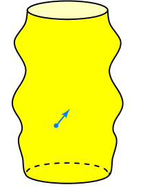
Figure 1: A supersymmetric particle propagating on a rigid wiggly cylinder. The bosonic degrees of freedom describe the position of the particle on the cylinder, $T_{1}$ is the axial coordinate, and $T_{2}$ is the angular coordinate. The fermionic degrees of freedom $\chi_{i}$ describe an internal “state” of the particle, which one can interpret in terms of target-space spinor components. The radius of the cylinder is $R(T_{1})=h(T_{1})^{1/2}$.

In this case, the complete supersymmetric Lagrangian turns out to be

$$L = {\textstyle\frac{1}{2}}\,\dot{T}_{1}^{2}-{\textstyle\frac{1}{2}}\,i\,\chi_{1}^{\dagger}\stackrel{{\scriptstyle\leftrightarrow}}{{\partial}}_{t}\chi_{1}+{\textstyle\frac{1}{2}}\,B_{1}^{2}$$ (7)

$$+h(T_{1})\,\Big{(}\,{\textstyle\frac{1}{2}}\,\dot{T}_{2}^{2}-{\textstyle\frac{1}{2}}\,i\,\chi_{2}^{\dagger}\stackrel{{\scriptstyle\leftrightarrow}}{{\partial}}_{t}\chi_{2}+{\textstyle\frac{1}{2}}\,B_{2}^{2}\,\Big{)}$$

$$+i\,h^{\prime}(T_{1})\,\chi_{[1}^{\dagger}\chi_{2]}\,\dot{T}_{2}-{\textstyle\frac{1}{2}}\,h^{\prime\prime}(T_{1})\,\chi_{2}^{\dagger}\chi_{2}\chi_{1}^{\dagger}\chi_{1}$$

$$+{\textstyle\frac{1}{2}}\,h^{\prime}(T_{1})\,\Big{(}\,\chi_{1}^{\dagger}\chi_{2}\,B_{2}+\chi_{2}^{\dagger}\chi_{1}\,B_{2}-\chi_{2}^{\dagger}\chi_{2}\,B_{1}\,\Big{)}$$

$$-{\textstyle\frac{1}{2}}\,\mu\,i\,h^{\prime}(T_{1})\,(\,\chi_{1}\,\chi_{2}+\chi_{1}^{\dagger}\chi_{2}^{\dagger}\,)-{\textstyle\frac{1}{2}}\,\mu^{2}\,h(T_{1})\,.$$

The final line in (7) describes those special terms needed to maintain supersymmetry in the presence of the inhomogeneous term in the transformation rules (4). At this point, the real parameter $\mu$ enters the action as an arbitrary coupling strength; it has been introduced for the express purpose of inserting a central charge into the superalgebra. A model of our sort is specified by a choice of the parameter $\mu$ and by a choice of the background “wiggle” function $h(T_{1})$.

The Dirac brackets derived from (7) provide the basic commutator and anti-commutator relationships which must be satisfied by the quantum operators corresponding to the canonical variables $T^{i}$, $P_{i}$, $\chi^{i}$ and $\chi^{i\,\dagger}$ . In our case, the relevant expressions are

$$[\,P_{i}\,,\,T^{j}\,] = -i\,\delta_{i}\,^{j}$$

$$\{\,\chi^{i}\,,\,\chi^{j\,\dagger}\,\} = G^{ij}$$

$$[\,P_{1}\,,\,\chi^{2}\,] = {\textstyle\frac{1}{2}}\,i\,\frac{h^{\prime}}{h}\,\chi^{2}\,,$$ (8)

where $G^{ij}$ is the inverse of the target-space metric $G_{ij}$. All other basic (anti)commutators vanish. The first two lines in (8) are generic, and the third is specific to the cylindrical geometry we have chosen in (6). Together, these determine $P_{i}=-i\,\partial_{i}$ and

$$\chi^{1} = {\textstyle\frac{1}{2}}\,(\Gamma^{3}+i\,\Gamma^{4}\,)$$

$$\chi^{2} = {\textstyle\frac{1}{2}}\,h^{-1/2}\,(\Gamma^{1}+i\,\Gamma^{2}\,)\,,$$ (9)

where $\Gamma^{\mu}$ are Euclidean Dirac matrices, which satisfy the four-dimensional Clifford algebra $\{\,\Gamma^{\mu}\,,\,\Gamma^{\nu}\,\}=2\,\delta^{\mu\nu}$.

We determine the quantum operators corresponding to the conserved charges after first eliminating the auxiliary fields $B_{1}$ and $B_{2}$. The supercharge operator, in this case, is given by

$$Q = P_{1}\,\chi_{1}+P_{2}\,\chi_{2}+{\textstyle\frac{1}{2}}\,i\,h^{\prime}:\chi_{2}\,\chi_{2}^{\dagger}\,\chi_{1}:+\mu\,h\,\chi_{2}^{\dagger}\,,$$ (10)

and the central charge operator is given by

$$Z=\mu\,P_{2}\,.$$ (11)

These are the operator analogs of the classical supercharges determined from (7) using the Noether procedure. The ordering ambiguity in the fermion cubic term is resolved by imposing the superalgebra on the quantum operators. The quantum Hamiltonian is

$$H = {\textstyle\frac{1}{2}}\,P_{1}^{2}+\frac{1}{2\,h}\,P_{2}^{2}-i\,\frac{h^{\prime}}{h}\,P_{2}\,\chi_{[1}^{\dagger}\chi_{2]}+{\textstyle\frac{1}{2}}\,:h\,{\cal R}\,\chi_{1}^{\dagger}\chi_{1}\chi_{2}^{\dagger}\chi_{2}:$$ (12)

$$+{\textstyle\frac{1}{2}}\,i\,\mu\,h^{\prime}\,(\,\chi_{1}\,\chi_{2}+\chi_{1}^{\dagger}\chi_{2}^{\dagger}\,)+{\textstyle\frac{1}{2}}\,\mu^{2}\,h\,,$$

where ${\cal R}$ is the scalar curvature on the target space. In terms of the metric function $h(T_{1})$, this is given by

$${\cal R}={\textstyle\frac{1}{2}}\,\Big{(}\,\frac{h^{\prime}}{h}\,\Big{)}^{2}-\frac{h^{\prime\prime}}{h}\,.$$ (13)

The term in the Hamiltonian (12) implicitly proportional to $h^{\prime\prime}$ arises from the explicit fermion quartic in the Lagrangian (7), while the other implicit fermion quartic term arises after elimination of the auxiliary fields $B_{i}$. Accordingly, there are two independent ordering ambiguities in the fermion quartic terms in (12). These, too, are resolved by imposing the superalgebra (1) on the quantum operators. (This determines Weyl ordering on the fermion cubic term in $Q$ and determines the particular ordering on the fermion quartics in $H$ reflected in the expressions which follow.)

It is useful to choose a particular representation for the fermions. A convenient choice is given by

$$\Gamma^{1,2,3}=\left(\begin{array}[]{c|c}&\sigma_{1,2,3}\\ \hline\cr\sigma_{1,2,3}&\end{array}\right)\hskip 14.45377pt\Gamma^{4}=\left(\begin{array}[]{c|c}&-i\,{\bf 1}\\ \hline\cr i\,{\bf 1}&\end{array}\right)\,,$$ (18)

where $\sigma_{1,2,3}$ are the Pauli matrices. However, the properly-ordered Hamiltonian is not diagonal in this basis. A diagonal Hamiltonian is obtained by first computing the Hamiltonian in the basis (18), resolving the ordering ambiguities as described above, and then performing on all operators ${\cal O}$ the similarity transformation ${\cal O}\to\check{\cal O}=\Lambda^{-1}\,{\cal O}\,\Lambda$, where

$$\Lambda=\frac{1}{\sqrt{2}}\,\left(\begin{array}[]{cc|cc}1&0&-i&0\\ i&0&-1&0\\ \hline\cr 0&1&0&i\\ 0&i&0&1\end{array}\right)\,.$$ (23)

Now, since $h(T_{1})^{1/2}$ is the radius of the cylinder, define $R(T_{1})\equiv h(T_{1})^{1/2}$. Also, since $T_{2}$ is an angular coordinate, it follows that the angular momentum $P_{2}$ is quantized, $P_{2}\equiv\nu\in\mathbb{Z}$. In terms of these definitions, after some algebra, one can write the Hamiltonian associated with the sector having angular momentum $\nu$ as

$$\check{H}=\left(\begin{array}[]{cc|cc}A_{+}^{\dagger}\,A_{+}+\mu\,\nu&&&\\ &A_{+}\,A_{+}^{\dagger}+\mu\,\nu&&\\ \hline\cr&&A_{-}^{\dagger}\,A_{-}+\mu\,\nu&\\ &&&A_{-}\,A_{-}^{\dagger}+\mu\,\nu\end{array}\right)\,,$$ (28)

where the operators $A_{\pm}$ are given by

$$A_{\pm}=\partial_{1}+W^{\prime}_{\pm}(T_{1})\,,$$ (29)

and the functions $W_{\pm}(T_{1})$ are superpotentials induced by the background wiggle function $h(T_{1})$ and also by the central charge. These are given by

$$W^{\prime}_{\pm}(T_{1}) = -\frac{1}{2}\,\frac{R^{\prime}}{R}\pm\,\Big{(}\,\frac{\nu}{R}-\mu\,R\,\Big{)}\,.$$ (30)

The four “sectors” of the Hamiltonian (12), which we enumerate using an index $n$, each include a distinct scalar potential $V_{n}(T_{1})$, determined from one of the superpotentials described by (30). There is an analogous four-sector Hamiltonian for each angular momentum sector, as labelled by the quantum number $\nu$.

The Hamiltonian (28) has several features worthy of note. First, and foremost, the class of models we have introduced include a manifest target-space duality. Under the simultaneous transformations

$$R \rightarrow \frac{1}{R}$$

$$\mu \leftrightarrow \nu$$

$$T_{1} \to -T_{1}\,,$$ (31)

all of the operators presented above transform simply. In particular, when $R(T_{1})=R(-T_{1})$, the transformation (31) leaves each of the operators $A_{\pm}$ multiplied by an overall minus sign, while for $R(T_{1})=-R(-T_{1})$, the operators $A_{\pm}$ map into each other. Thus, in these two cases, we have an explicit invariance of the Hamiltonian (28) under the mapping (31).

Because the duality map (31) includes a swapping of $\nu$ and $\mu$, a more precise statement is that it connects the angular momentum sector $P_{2}=\nu$ in a model with central charge parameter $\mu$ with the angular momentum sector $P_{2}=\mu$ in a model with central charge parameter $\nu$. If one interprets the quantum Hamiltonian (12) in terms of the sigma-model Lagrangian presented previously, $\nu$ is a quantized angular momentum, while $\mu$ is an arbitrary real parameter neither a priori quantized nor summed over. The duality relationship, as stated above, makes sense only if $\mu$ assumes integer values, however. This suggests to us the interesting possibility of an overarching theory, yet to be discovered, in which $\mu$ appears as an integer-valued topological quantity, properly summed over in the quantum theory. In such a construction, the exchange $\mu\leftrightarrow\nu$ would shuffle different sectors of the same theory, and the mapping $R(T_{1})\rightarrow 1/R(-T_{1})$ would itself describe an invariance, since the theory would automatically contain separate sums over the $\mu$ sectors and the $\nu$ sectors.

Looking at the superpotential functions (30), one is also struck by the following observation: a global re-scaling of $R$ is equivalent to separate re-scalings of $\mu$ and $\nu$ which leaves the product $\mu\,\nu$ fixed. In other words, the Hamiltonian (12) has yet another invariance, as described by the operation

$$R \to \lambda\,R$$

$$\nu \to \lambda\,\nu$$

$$\mu \to \lambda^{-1}\,\mu\,,$$ (32)

where $\lambda$ is an arbitrary real parameter. In this model, the mapping $\nu\rightarrow\nu+1$ already shifts among sectors, and if there is an overarching theory, there would be a sum over quantized $\mu$ values as well. These observations are consistent with the possibility that in the putative über-theory, the quantities $\mu$ and $\nu$ appear as an electric and magnetic charge-pair, related to each other by an $SL(\,2\,,\,\mathbb{Z}\,)$ transformation analogous to a generalized electric-magnetic duality.

We have exhibited a manifest “T-duality” and have motivated a prospective “S-duality” in a context we find elegant in its simplicity. The appearance of a target-space duality within non-relativistic point-particle quantum mechanics is itself surprising. But we also notice intriguing parallels with string theory. In the latter context, background geometry is famously restricted by quantum consistency conditions, conditions which are connected both to T-duality and to modular invariance. In the simpler models described in this paper, we also question what conditions might constrain the background geometry. Restrictions based on the duality structures described above form an attractive basis for such speculation. Another possibility we find intriguing is based on shape invariance. As described at the beginning of this paper, centrally-extended super-algebras, which form the basis of our investigation, also comprise the natural context for shape invariant extensions to any solvable quantum mechanics [8]. As it turns out, only particular background geometries can produce shape-invariant Hamiltonians of the form (12). Thus, we find that shape invariance, and the exact solubility to which it is associated, form an appealing mechanism for restricting the background geometry in which a supersymmetric particle can propagate. In light of this, we are led to attempt to ponder the possibility of connections between shape-invariant world-line dynamics and an eventual elemental description of M-theory.

Acknowledgements
The authors are grateful to Ted Allen for careful tutelage into the vagaries of Dirac brackets and constrained dynamics, which proved most helpful in our analysis. M.F. is also grateful to Mária and Emil Martinka, for hospitality, encouragement and halušky at the Slovak Institute for Basic Research, Podvazie Slovakia, where some of this work was performed.

References

- [1] E. Alvarez, L. Alvarez-Gaumé and Y. Lozano, An introduction to T duality in string theory, Nucl. Phys. Proc. Suppl. 41 (1995) 1.
- [2] E. Witten, Dynamical Breaking of Supersymmetry, Nucl. Phys. B188 (1981) 513-554.
- [3] E. Witten and D. Olive, Supersymmetry Algebras that include Topological Charges, Phys. Lett. B78 (1978) 97.
-
[4]
Z. Hlousek and D. Spector,
Why Topological Charges Imply Extended Supersymmetry,
Nucl. Phys. B370 (1992) 143-164 ;
Z. Hlousek and D. Spector, Topological charges and central charges in 3+1 dimensional supersymmetry, Phys. Lett. B283 (1992) 75-79. - [5] N. Graham and R.L. Jaffe, Energy, Central Charge, and the BPS Bound for 1+1 Dimensional Supersymmetric Solitons, Nucl. Phys. B544 (1999) 432.
- [6] G. Gibbons and P. Townsend, A Bogmol’nyi Equation for Intersecting Domain Walls Phys. Rev. Lett. 83 (1999) 1727.
- [7] P.M. Saffin, Tiling With Almost BPS Junctions Phys. Rev. Lett. 83 (1999) 4249.
- [8] M.Faux and D.Spector, An Algebraic Basis for Energy Bounds in Shape-Invariant Supersymmetric Quantum Mechanics, HWS-2003B11.
- [9] L. Infeld and T.D. Hull, The Factorization Method, Rev. Mod. Phys 23 (1951) 21-68.
- [10] L. Gendenshtein, Derivation of Exact Spectra of the Schrödinger Equation by Means of Supersymmetry, JETP Lett. 38 (1983) 356-359.
- [11] F. Cooper, J.N. Ginocchio and A. Khare, Relationship between supersymmetry and solvable potentials, Phys. Rev. D36 (1986) 2485-2473.
- [12] F. Cooper, A. Khare, and U. Sukhatme, Supersymmetry and Quantum Mechanics, Phys. Rept. 251 (1995) 267.