Wavelet based regularization for Euclidean field theory and stochastic quantization

Abstract

It is shown that Euclidean field theory with polynomial interaction, can be regularized using the wavelet representation of the fields. The connections between wavelet based regularization and stochastic quantization are considered with $\phi^{3}$ field theory taken as an example.

1 Introduction

The intimate connection between quantum field theory and stochastic differential equations has called constant attention for quite a long time [1, 2]. Among different aspects of this connection the stochastic quantization, proposed by G.Parisi and Y.Wu [3], is especially important, for it is believed to provide a new approach to quantization of Euclidean fields alternative to path integrals and canonical quantization. The stochastic quantization is also particularly attractive for quantization of gauge theories as it does not require gauge fixing. Besides that, the stochastic quantization procedure being based on random processes, and therefore on the measure theory, may be considered as a measure based formalism for constructing divergence free theory from beginning, instead of artificial regularization of the Riemann integrals in Euclidean space.

We know that stochastic processes often posses self-similarity. The renormalization procedure used in quantum field theory is also based on self-similarity. So, it is natural to use for the regularization of field theories the wavelet transform (WT), the decomposition with respect to the representation of the affine group. In this paper two ways of wavelet based regularization are presented. First, the direct substitution of WT of the fields into the action functional leads to a field theory with scale-dependent coupling constants. Second, the WT, being substituted into the Parisi-Wu stochastic quantization scheme [3], provides a stochastic regularization with no extra vertexes introduced into the theory.

2 Scalar field theory on affine group

The scalar field theory with the polynomial interaction $V(\phi)$ defined on Euclidean space $\mathbb{R}^{d}$ is one of the most instructive models any textbook in field theory starts with, see e.g.  [4]. This field theory is defined by the generating functional

$$W_{E}[J]={\cal N}\int{\cal D}\phi\exp\left[-S_{E}[\phi(x)]+\int d^{d}xJ(x)\phi(x)\right],$$ (1)

where $S_{E}[\phi(x)]$ is Euclidean action, ${\cal N}$ is formal normalization constant. The (connected) Green functions ($m$-point cumulative moments) are evaluated as functional derivatives of the logarithm of generating functional $W_{E}[J]=e^{-Z_{E}[J]}$:

$$G_{m}(x_{1},\ldots x_{m})\equiv\langle\phi(x_{1})\ldots\phi(x_{m})\rangle=-\left.\frac{\delta^{m}}{\delta J(x_{1})\ldots\delta J(x_{m})}\right|_{J=0}\ln W_{E}[J].$$ (2)

The generating functional (1) describes a quantum field $\phi(x)$ with the action

$$S_{E}[\phi]=\int_{\mathbb{R}^{d}}d^{d}x\left[{\frac{1}{2}(\partial_{\mu}\phi)^{2}+\frac{m^{2}}{2}\phi^{2}+\lambda V(\phi)}\right].$$ (3)

Alternatively, the theory of quantum field in Euclidean space is equivalent to the theory of classical fluctuating field with the Wiener probability measure ${\cal D}P=e^{-S_{E}[\phi]}{\cal D}\phi$. In this case $m^{2}=|T-T_{c}|$ is the deviation from critical temperature and $\lambda$ is the fluctuation interaction strength.

In the simplest case of a scalar field with the fourth power interaction

$$S_{E}[\phi]=\int d^{d}x\left[{\frac{1}{2}(\partial_{\mu}\phi)^{2}+\frac{m^{2}}{2}\phi^{2}+\frac{\lambda}{4!}\phi^{4}}\right]$$ (4)

the theory is often referred to as the Ginsburg-Landau model for its ferromagnetic applications. The $\phi^{3}$ theory is also a useful toy model used, for instance, to describe electron-phonon interactions [5].

The straightforward way to calculate the Green functions is to factorize the interaction part of generation functional (1) in the form

$$W_{E}[J]=\exp\left[-V\left(\frac{\delta}{\delta J}\right)\right]\exp\left(-\frac{1}{2}JD^{-1}J\right),\quad D=-\partial^{2}+m^{2}$$ (5)

The perturbation expansion is then evaluated in $k$-space, where

$${\widehat{D}}^{-1}(k)=\frac{1}{k^{2}+m^{2}}.$$

From group theory point of view the reformulation of a field theory from the coordinate representation $\phi(x)$ to the momentum representation $\hat{\phi}(k)$ by means of Fourier transform $\hat{\phi}(k)=\int_{\mathbb{R}^{d}}e^{\imath kx}\phi(x)d^{d}x$, is only a particular case of decomposition of a function with respect to representation of a Lie group $G$. For the Fourier transform $G$ is just an abelian group of translations, but other groups may be used as well, depending on the physics of a particular problem.

For a locally compact Lie group $G$ acting transitively on the Hilbert space ${\cal H}$ it is possible to decompose vectors $\phi\in{\cal H}$ with respect to the square-integrable representations $U(g)$ of the group $G$ [6, 7]:

$$|\phi\rangle=C_{\psi}^{-1}\int_{G}|U(g)\psi\rangle d\mu(g)\langle\psi U^{*}(g)|\phi\rangle,$$ (6)

where $d\mu(g)$ is the left-invariant Haar measure on $G$. The normalization constant $C_{\psi}$ is determined by the norm of the action of $U(g)$ on the fiducial vector $\psi\!\in\!{\cal H}$, i.e.  any $\psi\!\in\!{\cal H}$, that satisfies the admissibility condition

$$C_{\psi}:=\|\psi\|^{-2}\int_{g\in G}|\langle\psi|U(g)\psi\rangle|^{2}d\mu(g)<\infty,$$ (7)

can be used as a basis of wavelet decomposition.

In operator notation the decomposition (6) is also referred to as a partition of unity with respect to the representation $U(g)$:

$$\hat{1}=C_{\psi}^{-1}\int_{G}|U(g)\psi\rangle d\mu(g)\langle\psi U^{*}(g)|.$$

It is apparently possible to generalize the Feynman-Dyson perturbation expansion in a given field theory $S_{E}(\phi)$ by using decomposition (6) for non-abelian groups.

For definiteness, let us consider the fourth power interaction model with the (Euclidean) action functional

$$\begin{array}[]{lcl}S[\phi]&=&\frac{1}{2}\int_{\mathbb{R}^{d}}\phi(x_{1})D(x_{1},x_{2})\phi(x_{2})dx_{1}dx_{2}\\ &+&\frac{\lambda}{4!}\int V(x_{1},x_{2},x_{3},x_{4})\phi(x_{1})\phi(x_{2})\phi(x_{3})\phi(x_{4})dx_{1}dx_{2}dx_{3}dx_{4},\end{array}$$ (8)

where $D(x_{1},x_{2})$ is the inverse propagator of the free model ($\lambda\!=\!0$). Using the notation

$$U(g)|\psi\rangle\equiv|g,\psi\rangle,\quad\langle\phi|g,\psi\rangle\equiv\phi(g),\quad\langle g_{1},\psi|D|g_{2},\psi\rangle\equiv D(g_{1},g_{2}),$$

we can rewrite the generating functional (1) of the field theory with action (8) in the form

$$\begin{array}[]{lcl}W_{G}[J(g)]&=&\int{\cal D}\phi(g)\exp\Bigl{(}-\frac{1}{2}\int_{G}\phi(g_{1})D(g_{1},g_{2})\phi(g_{2})d\mu(g_{1})d\mu(g_{2})\\ &-&\frac{\lambda_{0}}{4!}\int_{G}\tilde{V}(g_{1},g_{2},g_{3},g_{4})\phi(g_{1})\phi(g_{2})\phi(g_{3})\phi(g_{4})d\mu(g_{1})d\mu(g_{2})d\mu(g_{3})d\mu(g_{4})\\ &+&\int_{G}J(g)\phi(g)d\mu(g)\Bigr{)},\end{array}$$ (9)

where

$$\begin{array}[]{lcl}\tilde{V}(g_{1},g_{2},g_{3},g_{4})&=&\int_{\mathbb{R}^{d}}V(x_{1},x_{2},x_{3},x_{4})(U(g_{1})\psi(x_{1}))(U(g_{2})\psi(x_{2}))\\ &&(U(g_{3})\psi(x_{3}))(U(g_{4})\psi(x_{4}))dx_{1}dx_{2}dx_{3}dx_{4}\end{array}$$

is the result of application of the wavelet transform in all arguments of $V$.

At this point we ought mention a real-world problem arising from substitution of the functional integration over physical fields by integration over the fields defined on a Lie group $G$. For the abelian group of translations (homeomorphic to $\mathbb{R}^{d}$) the inverse transform from Euclidean space to Minkovski space by changing $t$ into $\imath\!t$ does not yield any problems with causality, since the chronological ordering of operators is easily imposed. For non-abelian groups it is not clear how to order, or how to commute, the operator-valued fields at different points of the Lie group manifold $[\phi(g_{1}),\phi(g_{2})]=?$. This is an obstacle preventing quantization of gauge theories using wavelets [8]. That is why we will further consider only $c$-valued fields, bearing in mind the interpretation of Euclidean field theory in terms of the models of statistical mechanics.

Let us turn to the particular case of the affine group that is of our principle interest

$$x^{\prime}=aR(\theta)x+b,\quad R(\theta)\in SO_{d},x,x^{\prime},b\in\mathbb{R}^{d}.$$

Hereafter we assume the basic wavelet $\psi$ is invariant under $SO_{d}$ rotations $\psi(\mathbf{x})=\psi(|\mathbf{x}|)$ and drop the angular part of the measure for simplicity. After this simplifying assumption, the left-invariant Haar measure on affine group is $d\mu(a,{\bm{b}})=\frac{dad^{d}{\bm{b}}}{a^{d+1}}$. The representation $U(g)$ induced by a basic wavelet $\psi(x)$ is

$$g:{\bm{x}}^{\prime}=a{\bm{x}}+{\bm{b}},\quad U(g)\psi({\bm{x}})=a^{-d/2}\psi\left(\frac{{\bm{x}}-{\bm{b}}}{a}\right).$$ (10)

The (bold) vector notation is dropped where it does not lead to confusion. The last thing we need to construct the generating functional of a field theory on affine group is to substitute wavelet decomposition

$$\phi(x)=C_{\psi}^{-1}\int a^{-d/2}\psi\left(\frac{x-b}{a}\right)\phi_{a}(b)\frac{dad^{d}b}{a^{d+1}},$$ (11)

into Euclidean action $S_{E}[\phi]$. Here we use normalization for the rotationally invariant wavelets

$$C_{\psi}=\int\frac{|\hat{\psi}(k)|^{2}}{S_{d}|k|^{d}}d^{d}k,$$ (12)

where the area of the unit sphere in $d$ dimensions $S_{d}$ has come from rotation symmetry. The wavelet coefficients

$$\phi_{a}(b)=\int a^{-d/2}\bar{\psi}\left(\frac{x-b}{a}\right)\phi(x)d^{d}x$$ (13)

represent the snapshot of the field $\phi(x)$ taken at the scale $a$ with the aperture function $\psi(x)$, and will be referred to as scale components of the field $\phi$. See e.g. [9] for more details on wavelets.

The restriction imposed by the admissibility condition (7) on the fiducial vector $\psi$ (the basic wavelet) is rather loose: only the finiteness of the integral $C_{\psi}$ given by (12) is required. This practically implies only that $\int\psi(x)dx=0$ and that $\psi(x)$ has compact support. For this reason the wavelet transform (13) can be considered as a microscopic slice of the function $\phi(x)$ taken at a position $b$ and resolution $a$ with “aperture” $\psi$. Of course, each particular aperture $\psi(x)$ has its own view, but the physical observables should be independent on it. In practical applications of WT either of the derivatives of the Gaussian $\psi_{n}(x)=(-1)^{n}d^{n}/dx^{n}e^{-x^{2}/2}$ are often used, but for the purpose of this present paper only the admissibility condition is important but not the shape of $\psi(x)$.

So, for the case of decomposition of a scalar field in $\mathbb{R}^{d}$ with respect to affine group (10), the inverse free field propagator matrix element is

$$\langle a_{1},b_{1};\psi|D|a_{2},b_{2};\psi\rangle=\int d^{d}x(a_{1}a_{2})^{-\frac{d}{2}}\bar{\psi}\left(\frac{x-b_{1}}{a_{1}}\right)D\psi\left(\frac{x-b_{2}}{a_{2}}\right)$$

$$=\int\frac{d^{d}{k}}{(2\pi)^{d}}e^{ik(b_{1}-b_{2})}(a_{1}a_{2})^{\frac{d}{2}}\overline{\hat{\psi}(a_{1}k)}(k^{2}+m^{2})\hat{\psi}(a_{2}k)$$

$$\equiv\int\frac{d^{d}{k}}{(2\pi)^{d}}e^{ik(b_{1}-b_{2})}D(a_{1},a_{2},k).$$

Assuming the homogeneity of the free field in space coordinate, i.e. that matrix elements depend only on the differences $(b_{1}\!-\!b_{2})$ of the positions, but not the positions themselves, we can use $(a,k)$ representation:

$$D(a_{1},a_{2},k) = a_{1}^{d/2}\overline{\hat{\psi}(a_{1}k)}(k^{2}+m^{2})a_{2}^{d/2}\hat{\psi}(a_{2}k)$$

$$D^{-1}(a_{1},a_{2},k) = a_{1}^{d/2}\overline{\hat{\psi}(a_{1}k)}\left(\frac{1}{k^{2}+m^{2}}\right)a_{2}^{d/2}\hat{\psi}(a_{2}k)$$ (14)

$$d\mu(a,k) = \frac{d^{d}{k}}{(2\pi)^{d}}\frac{d{a}}{{a}^{{d}+1}}.$$

Thus, we have the same diagram technique as usually, but with extra “wavelet” term $a^{d/2}\hat{\psi}(ak)$ term on each line and the integration over $d\mu(a,k)$ instead of $dk$.

Now, turning back to the coordinate representation (13), where $a$ is the resolution (“window width”) and recalling the power law dependence resulted from the Wilson expansion, we can define the $\phi^{4}$ model on affine group, with the coupling constant dependent on scale. The simplest case of the fourth power interaction of this type is

$$V_{int}[\phi]=\int\frac{\lambda(a)}{4!}\phi^{4}_{a}(b)d\mu(a,b),\quad\lambda(a)\sim a^{\nu}.$$ (15)

The one-loop order contribution to the Green function $G_{2}$ in the theory with interaction (15) can be easily evaluated [10] by integration over a scalar variable $z=ak$:

$$\int\frac{a^{\nu}a^{d}|\hat{\psi}(ak)|^{2}}{k^{2}+m^{2}}\frac{d^{d}{k}}{(2\pi)^{d}}\frac{d{a}}{{a}^{{d}+1}}=C_{\psi}^{(\nu)}\int\frac{d^{d}{k}}{(2\pi)^{d}}\frac{k^{-\nu}}{k^{2}+m^{2}},$$ (16)

where

$$C_{\psi}^{(\nu)}=\int|\hat{\psi}(z)|^{2}z^{\nu-1}dz.$$

Therefore, there are no UV divergences for $\nu>d\!-\!2$.

However, the positive values of $\nu$ mean that the interaction strengths at large scales and diminishes at small. This is a kind of asymptotically free theory that is hardly appropriate say to magnetic systems. What is required instead is a theory with the interaction vanishing outside a given domain of scales. Such models will be presented in the next section by means of scale-dependent stochastic quantization.

3 Stochastic quantization with wavelets

The method of stochastic quantization first introduced by G.Parisi, and Y.Wu [3] consists in substitution of functional integration by averaging over certain random process. Let $S_{E}[\phi]$ be the action Euclidean field theory (3) in $\mathbb{R}^{d}$. Then, instead of direct calculation of the Green functions (2) from the generation functional (1), it is possible to introduce a fictitious “time” variable $\tau$, make the quantum fields into stochastic fields $\phi(x)\to\phi(x,\tau),x\!\in\!\mathbb{R}^{d},\tau\!\in\!\mathbb{R}$ and evaluate the moments $\langle\phi(x_{1},\tau_{1})\ldots\phi(x_{m},\tau_{m})\rangle$ by averaging over a random process $\phi(x,\tau,\cdot)$ governed by the Langevin equation

$$\frac{\partial\phi(x,\tau)}{\partial\tau}+\frac{\sigma^{2}}{2}\frac{\delta S}{\delta\phi(x,\tau)}=\eta(x,\tau).$$ (17)

The gaussian random force $\eta$, that drives the Langevin equation (17), has zero mean and is $\delta$-correlated in both the $\mathbb{R}^{d}$ coordinate and the fictitious time:

$$\langle\eta(x,\tau)\rangle=0,\quad\langle\eta(x,\tau)\eta(x^{\prime},\tau^{\prime})\rangle=\sigma^{2}\delta(x-x^{\prime})\delta(\tau-\tau^{\prime}).$$ (18)

The physical Green functions are obtained by taking the steady state limit

$$G(x_{1},\ldots,x_{m})=\lim_{\tau\to\infty}\langle\phi(x_{1},\tau)\ldots\phi(x_{m},\tau)\rangle$$ (19)

either in the solution of the Fokker-Planck equation, or in the stochastic perturbation expansion given by stochastic generating functional

$$W[J(x,\tau)]=\int{\cal D}\phi{\cal D}\eta\exp\left[{\int d^{d}xd\tau\left(J\phi-\frac{\eta^{2}}{2\sigma^{2}}\right)}\right]\delta\left[{\frac{\partial\phi}{\partial\tau}+\frac{\sigma^{2}}{2}\frac{\delta S}{\delta\phi}-\eta}\right].$$ (20)

The stochastic quantization procedure has been considered as perspective candidate for the regularization of gauge theories, for it does not require gauge fixing. However $\delta$-correlated Gaussian random force in the Langevin equation still yields singularities in the perturbation theory. For this reason a number of modifications based on the noise regularization $\eta(x,\tau)\to\int dyR_{xy}(\partial^{2})\eta(y,\tau)$ have been proposed [11, 12, 13]. The introduction of a colored noise $\langle\eta(x,\tau)\eta(x^{\prime},\tau^{\prime})\rangle=\delta(x-x^{\prime})|\tau-\tau^{\prime}|^{n}$ instead of $\delta$-correlated one can be also used to avoid UV divergences [11, 14]. Other methods of regularization in stochastically quantized theories were also considered [15, 16].

In this paper we intend to revive the method of stochastic quantization by applying the continuous wavelet transform to both the fields $\phi(x,\tau)$ and the random force $\eta(x,\tau)$. It will be shown that ultra-violet divergences in so constructed perturbation expansion can be eliminated for some particular choice of the random force correlator taken in wavelet space. Our method is rather general and can be applied to any stochastic systems described by the Langevin equation. The idea of our method was proposed in [17] and consists in the following.

Instead of the usual space of the random functions $f(x,\cdot)\in(\Omega,{\cal A},P)$, where $f(x,\omega)\in{\rm L}^{2}({\mathbb{R}^{d}})$ for each given realization $\omega$ of the random process, we go to the multi-scale representation provided by the continuous wavelet transform (13):

$$W_{\psi}(a,{\bm{b}},\cdot)=\int|a|^{-\frac{d}{2}}\overline{\psi\left(\frac{{\bm{x}}-{\bm{b}}}{a}\right)}f({\bm{x}},\cdot)d^{d}x.$$ (21)

Since the structure of divergences and the localization of the solutions are determined by the spatial part of the random force correlator (see e.g.  [18]), the wavelet transform is performed only in the spatial argument $x\!\in\!\mathbb{R}^{d}$ of the dynamical variable $\phi(x,\tau)$, but not in its fictitious time argument.

The inverse wavelet transform

$$f({\bm{x}},\cdot)=C_{\psi}^{-1}\int|a|^{-\frac{d}{2}}\psi\left(\frac{{\bm{x}}-{\bm{b}}}{a}\right)W_{\psi}(a,{\bm{b}},\cdot)\frac{dad{\bm{b}}}{a^{d+1}}$$ (22)

reconstructs the common random process as a sum of its scale components, i.e.  projections onto different resolution spaces.

The use of the scale components instead of the original stochastic process provides an extra analytical flexibility of the method: there exist more than one set of random functions $W(a,{\bm{b}},\cdot)$ the images of which have coinciding correlation functions in the space of $f(x,\cdot)$. It is easy to check that the random process generated by wavelet coefficients having in $(a,k)$ space the correlation function

$$\langle\widehat{W}(a_{1},k_{1})\widehat{W}(a_{2},k_{2})\rangle=C_{\psi}(2\pi)^{d}\delta^{d}(k_{1}+k_{2})a_{1}^{d+1}\delta(a_{1}-a_{2})D_{0}$$ (23)

has the same correlation function as white noise has:

$$\begin{array}[]{lcl}\langle f(x_{1})f(x_{2})\rangle&=&D_{0}\delta^{d}(x_{1}-x_{2}),\\ \langle{\hat{f}}(k_{1})\hat{f}(k_{2})\rangle&=&(2\pi)^{d}D_{0}\delta^{d}(k_{1}+k_{2})\\ \langle\widehat{W}_{\psi}(a_{1},k_{1})\widehat{W}_{\psi}(a_{2},k_{2})\rangle&=&(2\pi)^{d}D_{0}\delta^{d}(k_{1}+k_{2})(a_{1}a_{2})^{d/2}\overline{\hat{\psi}(a_{1}k_{1})\hat{\psi}(a_{2}k_{2})}.\end{array}$$

Therefore, starting from a given random process in the space of scale-dependent functions $W(a,{\bm{b}},t)$, rather than in a common space of square integrable functions $f({\bm{x}},t)$, we can design a narrow band forcing with no contradictions to other physical constraints. This can be done by applying the requirement $W(a,{\bm{b}},t)\!\to\!0$ for all $a$ outside a certain domain of scales $[a_{min},a_{max}]$.

Now let us turn to the stochastic quantization of the $\phi^{3}$ theory with the help of scale-dependent noise designed in the above described way. The Euclidean action of the $\phi^{3}$ theory is

$$S_{E}[\phi(x)]=\int d^{d}x\left[\frac{1}{2}(\partial\phi)^{2}+\frac{m^{2}}{2}\phi^{2}+\frac{\lambda}{3!}\phi^{3}\right].$$ (24)

Therefore the corresponding Langevin equation used for stochastic quantization is written as

$$\frac{\partial\phi(x,\tau)}{\partial\tau}+\frac{D_{0}}{2}\left[-\Delta\phi+m^{2}\phi+\frac{\lambda}{2!}\phi^{2}\right]=\eta(x,\tau),$$ (25)

where in common case the $\delta$-correlated random force is applied

$$\langle\eta(x,\tau)\eta(x^{\prime},\tau^{\prime})\rangle=D_{0}\delta^{d}(x-x^{\prime})\delta(\tau-\tau^{\prime}).$$

Following [17], we perform continuous wavelet transform of the fields and forces in the spatial coordinate

$$\phi(x)=C_{\psi}^{-1}\int\exp(\imath({\bm{k}}{\bm{x}}-\omega\tau))a^{\frac{d}{2}}\hat{\psi}(a{\bm{k}})\hat{\phi}(a,k)\frac{d^{d+1}{k}}{(2\pi)^{d+1}}\frac{d{a}}{{a}^{{d}+1}},$$ (26)

using hereafter apparent $(d\!+\!1)$ dimensional notation $x=({\bm{x}},\tau),k=({\bm{k}},\omega)$. To generalize the scale-dependent force (23) we introduce dependence on $k$ in the force correlator

$$\begin{array}[]{lcl}\langle\widehat{\eta}(a_{1},k_{1})\widehat{\eta}(a_{2},k_{2})\rangle&=&C_{\psi}(2\pi)^{d+1}\delta^{d+1}(k_{1}+k_{2})a_{1}^{d+1}\delta(a_{1}-a_{2})2D(a_{2},{\bm{k}}_{2}),\\ \langle\hat{\eta}(a,k)\rangle&=&0,\end{array}$$ (27)

which coincides with (23) if $D(a,{\bm{k}})=const$, and is therefore capable of giving white noise in that limiting case. After substitution of (26) into the Langevin equation (25) we yield the stochastic integro-differential equation for stochastic fields $\hat{\phi}(a,k,\cdot)$

$$\begin{array}[]{l}(-\imath\omega+{\bm{k}}^{2}+m^{2})\hat{\phi}(a,k)=\hat{\eta}(a,k)-\frac{\lambda}{2}a^{\frac{d}{2}}\overline{\hat{\psi}(a{\bm{k}})}C_{\psi}^{-2}\int(a_{1}a_{2})^{\frac{d}{2}}\\ \hat{\psi}(a_{1}{\bm{k}}_{1})\hat{\psi}(a_{2}({\bm{k}}-{\bm{k}}_{1}))\hat{\phi}(a_{1},k_{1})\hat{\phi}(a_{2},k-k_{1})\frac{d^{d+1}{k_{1}}}{(2\pi)^{d+1}}\frac{d{a_{1}}}{{a_{1}}^{{d}+1}}\frac{d{a_{2}}}{{a_{2}}^{{d}+1}}.\end{array}$$ (28)

Starting from the zero-th order approximation $\hat{\phi}_{0}(a,k)=G_{0}(k)\hat{\eta}(a,k)$ with the bare Green function

$$G_{0}(k)=\frac{1}{-\imath\omega+{\bm{k}}^{2}+m^{2}}$$

and iterating the integral equation (28), in one loop approximation we get the correction to the stochastic Green function

$$G(k)=G_{0}(k)+\lambda^{2}G_{0}^{2}(k)\int\frac{d^{d+1}{q}}{(2\pi)^{d+1}}\Delta({\bm{q}})|G_{0}(q)|^{2}G_{0}(k-q)+O(\lambda^{4}),$$ (29)

where $\Delta({\bm{k}})$ is the scale averaged correlator (30):

$$\Delta({\bm{k}})\equiv C_{\psi}^{-1}\int\frac{da}{a}|\hat{\psi}(a{\bm{k}})|^{2}2D(a,{\bm{k}})$$ (30)

In the same way all other momenta (2) can be evaluated. Thus the common stochastic diagram technique is reproduced with the scale-dependent random force (27) instead of the standard one. The 1PI diagramms corresponding to the stochastic Green function decomposition (29) are shown in Fig. 1.

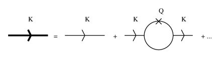
Figure 1: Diagramm expansion of the stochastic Green function in $\phi^{3}$-model

Similarly, to stochastic Green function (29), the one-loop contribution to the stochastic pair correlation function can be evaluated in $(a,k)$ space

$$\langle\hat{\phi}(a_{i},k)\hat{\phi}(a_{f},-k)\rangle\equiv C(a_{i},a_{f},k)=C_{0}(a_{i},a_{f},k)+\lambda^{2}C_{2}(a_{i},a_{f},k)+O(\lambda^{4}),$$ (31)

where

$$C_{0}(a_{i},a_{f},k)=\Delta({\bm{k}})|G_{0}(k)|^{2}(a_{i}a_{f})^{d/2}\overline{\hat{\psi}(a_{i}{\bm{k}})\hat{\psi}(-a_{f}{\bm{k}})}.$$

The one-loop contribution to the pair correlator is

$$C_{2}(a_{i},a_{f},k) = \frac{1}{2}|G_{0}(k)|^{2}(a_{i}a_{f})^{d/2}\overline{\hat{\psi}(a_{i}{\bm{k}})\hat{\psi}(-a_{f}{\bm{k}})}$$

$$\int\frac{d^{d+1}{q}}{(2\pi)^{d+1}}|G_{0}(q)|^{2}|G_{0}(k-q)|^{2}\Delta({\bm{q}})\Delta({\bm{k}}-{\bm{q}}).$$

The 1PI diagramms corresponding to the stochastic pair correlator decomposition (31) are shown in Fig. 2.

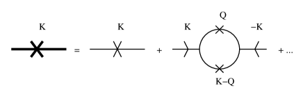
Figure 2: Diagramm expansion of the stochastic pair correlation function in $\phi^{3}$ model

An important type of scale-dependent forcing is that acting on a single scale:

$$D(a,{\bm{k}})=\delta(a-a_{0})D({\bm{k}}).$$ (33)

In some sense this mimics a field theory on a grid with a fixed mesh $a_{0}$.

As an example, let us consider the $\phi^{3}$ model with the single-scale force (33) and the “Mexican hat” used as a basic wavelet

$$\hat{\psi}(k)=(2\pi)^{d/2}(-\imath{\bm{k}})^{2}\exp(-{\bm{k}}^{2}/2),\quad C_{\psi}=(2\pi)^{d}.$$ (34)

This gives the effective force correlator

$$\Delta({\bm{q}})=2\frac{(a_{0}{\bm{q}})^{4}}{a_{0}}e^{-(a_{0}{\bm{q}})^{2}}D({\bm{q}}).$$ (35)

The loop integrals taken with this effective force correlator (35) can be easily seen to be free of ultra-violet divergences. The IR divergences also become milder because of the wavelet power factor $(a_{0}{\bm{q}})^{4}$.

In fact, substituting (35) into expressions for one-loop contributions to the stochastic Green function and the correlation functions, (29) and (3), respectively, we get

$$G_{2}(k) = G_{0}^{2}(k)I_{G2},$$ (36)

$$I_{G2} = \int\frac{d^{d}{{\bm{q}}}}{(2\pi)^{d}}\Delta({\bm{q}})\int_{-\infty}^{\infty}\frac{d\Omega}{2\pi}\frac{1}{\Omega^{2}+({\bm{q}}^{2}+m^{2})^{2}}\frac{1}{-\imath(\omega-\Omega)+({\bm{k}}-{\bm{q}})^{2}+m^{2}}$$

$$C_{2}(a_{i},a_{f},k) = \frac{1}{2}|G_{0}(k)|^{2}(a_{i}a_{f})^{d/2}\overline{\hat{\psi}(a_{i}{\bm{k}})\hat{\psi}(-a_{f}{\bm{k}})}I_{C2},$$ (37)

$$I_{C2} = \int\frac{d^{d}{{\bm{q}}}}{(2\pi)^{d}}\Delta({\bm{q}})\Delta({\bm{k}}-{\bm{q}})\int_{-\infty}^{\infty}\frac{d\Omega}{2\pi}\frac{1}{\Omega^{2}+({\bm{q}}^{2}+m^{2})^{2}}\frac{1}{(\omega-\Omega)^{2}+[({\bm{k}}-{\bm{q}})^{2}+m^{2}]^{2}}.$$

For the case of single-scale forcing (35) the exponential factor in $\Delta({\bm{q}})$ will suppress any power divergences comming from the Green functions. In fact, in a stationary limit ($\omega\!\to\!0$), after the integration over the frequency variable $\Omega$, we get

$$\lim_{\omega\to 0}I_{G2} = \int\frac{d^{d}{{\bm{q}}}}{(2\pi)^{d}}\Delta({\bm{q}})\frac{1}{2({\bm{q}}^{2}+m^{2})}\cdot\frac{1}{{\bm{q}}^{2}+({\bm{k}}-{\bm{q}})^{2}+2m^{2}}$$ (38)

$$\lim_{\omega\to 0}I_{C2} = \int\frac{d^{d}{{\bm{q}}}}{(2\pi)^{d}}\Delta({\bm{q}})\frac{1}{2({\bm{q}}^{2}+m^{2})(({\bm{k}}-{\bm{q}})^{2}+m^{2})}\cdot\frac{1}{{\bm{q}}^{2}+({\bm{k}}-{\bm{q}})^{2}+2m^{2}}.$$ (39)

An explicit calculation gives the frequency dependence:

$$I_{G2} = \frac{1}{2B}\frac{1}{(A-B)-\imath\omega}+\frac{1}{(\omega+\imath A)^{2}+B^{2}}$$

$$I_{C2} = \frac{1}{2A}\frac{1}{(\omega+\imath A)^{2}+B^{2}}+\frac{1}{2B}\frac{1}{(\omega-\imath B)^{2}+A^{2}}$$

where

$$A=({\bm{k}}-{\bm{q}})^{2}+m^{2},\quad B={\bm{q}}^{2}+m^{2}.$$

For the $\phi^{4}$ and higher polynomial models the above described method can be applied in a straightforward way.

4 Conclusion

In this paper, that is extended version of [19], we have presented a new approach to regularization of field theories based on wavelet decomposition of the fields. The idea of using the affine group in quantum field theory is not new. It is in the basis of the renormalization group method the modern quantum field theory resides on. However, the direct use of the representations of affine group as a basis in the space of wave functions can provide a new perspectives in construction of a divergence free field theory. From the point of view of functional analysis this is an extension of the space of square integrable functions $\phi(x)$ to the space of scale-dependent functions $\phi_{a}(x)$, representing a snapshots of the field $\phi$ at a given resolutions $a$. The usage of functions depending on scale suggests that the interaction potential should be scale-dependent too. Such potentials having been de facto already in use in renormalization group technique, can be directly incorporated into quantum field theory from beginning. One of means to do it is the method of scale dependent stochastic quantization proposed in this paper. Although direct construction of the quantum field theory on the affine group presented in the beginning of this paper is also possible.

References

• [1] E. Nelson. Quantum fluctuations. Princeton University Press, New Jersey, 1985.
• [2] J. Glim and A. Jaffe. Quantum physics. Springer-Verlag, NY, 1981.
• [3] G. Parisi and Y.-S. Wu. Perturbation theory without gauge fixing. Scientica Sinica, 24:483, 1981.
• [4] P. Ramond. Field Theory: A modern Primer. Benjamin/Cummings Publishing Company,Inc., Massachussets, 1981.
• [5] A.A. Abrikosov, L.P. Gorkov, and I.E. Dzaloshinskij. Quantum field theory methods in statistical physics. Dobrosvet, Moscow, second edition, 1998. (In Russian).
• [6] A.L. Carey. Square-integrable representations of non-unimodular groups. Bull. Austr. Math. Soc., 15:1–12, 1976.
• [7] M. Duflo and C.C. Moore. On regular representations of nonunimodular locally compact group. J. Func. Anal., 21:209–243, 1976.
• [8] P. Federbush. A new formulation and regularization of gauge theories using a non-linear wavelet expansion. Progr. Theor. Phys., 94:1135–1146, 1995.
• [9] C.K. Chui. An introduction to wavelets. Academic press, inc, 1991.
• [10] M.V. Altaisky. $\phi^{4}$ field theory on a lie group. In B.G. Sidharth and M.V. Altaisky, editors, Frontiers of fundamental physics 4, pages 124–128, NY, 2001. Kluver Academic / Plenum Publishers.
• [11] J. Breit, S. Gupta, and A. Zaks. Stochastic quantization and regularization. Nuclear Physics B, 233:61–68, 1984.
• [12] Z. Bern, M. Halpern, L. Sadun, and C. Taubes. Continuum regularization of quantum field theory (i). Scalar prototype. Nuclear Physics B, 284:1–91, 1987.
• [13] R. Iengo and S. Pugnetti. Stochastic quantization, non-Markovian reqularization and renormalization. Nuclear Physics B, 300, 1988.
• [14] J. Alfaro. Stochastic analytic regularization. Nuclear Physics B, 253(3/4):464–476, 1985.
• [15] M. Namiki and Y. Yamanaka. Stochastic quantization method in operator formalism. Progr. Theor. Phys., 69(6):1764–1793, 1983.
• [16] S. Chaturvedi, A.K. Kapoor, and V. Srinivasan. Renormalization of stochastically quantized fields. Int. J. Mod. Phys. A, 3(1):163–165, 1988.
• [17] M.V. Altaisky. Langevin equation with scale-dependent noise. Doklady Physics, 48(9):478–480, 2003.
• [18] M. Kardar, G. Parisi, and Y.-C. Zhang. Dynamic scaling of growing interfaces. Phys. Rev. Lett., 56(9):889–892, 1986.
• [19] M. Altaisky. Wavelet based regularization for Euclidean field theory. In J.-P. Gazeau, R. Kerner, J.-P. Antoine, and S. Metens, editors, Proc. Int. Conf. Group24: Physical and mathematical aspects of symmetries, Bristol, 2003. IOP Publishing.