Quantum gravity at a large number of dimensions

Abstract

We consider the large-$D$ limit of Einstein gravity. It is observed that a consistent leading large-$D$ graph limit exists, and that it is built up by a subclass of planar diagrams. The graphs in the effective field theory extension of Einstein gravity are investigated in the same context, and it is seen that an effective field theory extension of the basic Einstein-Hilbert theory will not upset the latter leading large-$D$ graph limit, i.e., the same subclass of planar diagrams will dominate at large-$D$ in the effective field theory. The effective field theory description of large-$D$ quantum gravity limit will be renormalizable, and the resulting theory will thus be completely well defined up to the Planck scale at $\sim 10^{19}$ GeV. The $\left(\frac{1}{D}\right)$ expansion in gravity is compared to the successful $\left(\frac{1}{N}\right)$ expansion in gauge theory (the planar diagram limit), and dissimilarities and parallels of the two expansions are discussed. We consider the expansion of the effective field theory terms and we make some remarks on explicit calculations of $n$-point functions.

I Introduction

A traditional belief is that an adequate description of quantum gravity is necessarily complicated, and that we are very far from a satisfying explanation of its true physical content. This might be correct, however progress on the problems in quantum gravity are being made, and gravitational interactions are today better understood than previously. The fate of gravity in the limit of Planckian scale energies is still unknown. At the physical transition to such energies $\sim 10^{19}$ GeV, fundamental issues are believed to arise. They concern the validity of the conceptual picture of space and time geometry. A completely new understanding of physics might be the consequence. String theory or the so called $M$-theory are candidates for such theories in high energy physics.

Einstein’s theory of general relativity on the other hand presents us with an excellent classical model for the interactions of matter and space-time in the low energy regime of physics. Astronomical observations support the theoretical predictions, and there are no experimental reasons for a disbelief in the physical foundations of general relativity. The fact that general relativity is not a quantum theory is however intriguing. A fundamental description of nature should either be completely classical or quantum mechanical from a theoretical point of view, and so far experiments support quantum mechanics as the correct basis for interpreting physical measurements. It would be nice to unify Einstein’s theory in the classical low energy limit with a full quantum field theoretic description in the high energy limit. This seems not to be immediately possible, attempts of making a quantum field theoretic description of general relativity have normally proven to be incomplete in regard to the question of renormalizability of the fundamental action for the theory. The basic four-dimensional Einstein-Hilbert action:

$${\cal L}_{\rm EH}=\int d^{4}x{\sqrt{-g}}\Big{(}\frac{2R}{\kappa^{2}}+{\cal L}_{\text{matter}}\Big{)},$$ (1)

is not renormalizable in the sense that the counter-terms which appear in the renormalized action, e.g., ($\sim R^{2}$), ($\sim R_{\mu\nu}R^{\mu\nu}$) and ($\sim R^{3}),\ \ldots$ cannot be absorbed in the original action Veltman ; NON ; matter . In the above equation ($\kappa^{2}$) is defined as ($32\pi G_{D}$), where ($G_{D}$) is the $D$-dimensional Newton constant. The disappointing conclusion is usually that a field theoretical treatment of gravity is not possible, and that one should avoid attempting such a description.

Effective field theory presents a solution to the renormalization problem of gravity. It initially originates from an idea put forward by Weinberg Weinberg . Including all possible invariants into the action, i.e., replacing the basic $D$-dimensional Einstein-Hilbert action with:

$${\cal L}_{\rm effective\ EH}=\int d^{D}x{\sqrt{-g}}\bigg{(}\Big{(}\frac{2R}{\kappa^{2}}+c_{1}R^{2}+c_{2}R^{\mu\nu}R_{\mu\nu}+\ldots\Big{)}+{\cal L}_{\text{eff. matter}}\bigg{)},$$ (2)

solves the issue of renormalizability. No counter terms can be generated in a covariant renormalization scheme, which are not already present in the action. The effective field theory approach will always lead to consistent renormalizable theories in any dimension, e.g., for ($D=4$), ($D=10$) or even ($D=127$). It is important to note that in regard to its renormalizability, an effective field theory in the large-$D$ limit of gravity is just as well defined as the planar diagram large-$N$ limit, in e.g., a $(D=4)$ Yang-Mills theory. A Yang-Mills theory, at ($D>4$), will also need to be treated by means of effective field theory in order to be renormalizable. What we give up in the effective field treatment of gravity or in any other theory, is the finite number of terms in the action. The Einstein action is replaced with an action which has an infinite number of coupling constants. These have to be renormalized at each loop order. The coupling constants of the effective expansion of the action, i.e., ($c_{1},c_{2},\ldots$), will have to be determined by experiment and are running, i.e., they will depend on the energy scale. However, the advantage of the effective approach is quite clear. Quantum gravity is an effectively renormalizable theory up to the energies at the Planck scale!

The effective field theory description of general relativity has directly shown its worth by explicit calculations of quantum corrections to the metric and to the Newtonian potential of large masses. This work was pioneered by Donoghue, refs. Donoghue:dn ; B1 ; B2 , and as an effective field theory combined with QED, refs. DB ; QED . The conceptual picture of Einstein gravity is not affected by the effective field theory treatment of the gravitational interactions. The equations of motion will of course be slightly changed by the presence of higher derivative terms in the action, however the contributions coming from such terms can at normal energies be shown to be negligible Stelle ; Simon:ic . Effective field theory thus provides us with a very solid framework in the study of gravitational interactions and quantum effects at normal energies, and solves some of the essential problems in building field theoretical quantum gravity models.

An intriguing paper by Strominger Strominger:1981jg deals with the perspectives of basic Einstein gravity at an infinite number of dimensions. The basic idea is to let the spatial dimension be a parameter in which one is allowed to expand the theory. Each graph of the theory is then associated with a dimensional factor. Formally one can expand every Greens function of the theory as a series in $\left(\frac{1}{D}\right)$ and the gravitational coupling constant ($\kappa$):

$$G=\sum_{i,j}(\kappa)^{i}\left(\frac{1}{D}\right)^{j}{\cal G}_{i,j}.$$ (3)

The contributions with highest dimensional dependence will be the leading ones in the large-$D$ limit. Concentrating on these graphs only simplifies the theory and makes explicit calculations easier. In the effective field theory we expect an expansion of the theory of the type:

$$G=\sum_{i,j,k}(\kappa)^{i}\left(\frac{1}{D}\right)^{j}({\cal E})^{2k}{\cal G}_{i,j,k},$$ (4)

where (${\cal E}$) represents a parameter for the effective expansion of the theory in terms of the energy, i.e., each derivative acting on a massless field will correspond to a factor of (${\cal E}$). The basic Einstein-Hilbert scale will correspond to the (${\cal E}^{2}\sim\partial^{2}g$) contribution, while higher order effective contributions will be of order (${\cal E}^{4}\sim\partial^{4}g$), (${\cal E}^{6}\sim\partial^{6}g$), $\ldots$ etc.

The idea of making a large-$D$ expansion in gravity is somewhat similar to the large-$N$ Yang-Mills planar diagram limit considered by ’t Hooft tHooft . In large-$N$ gauge theories, one expands in the internal symmetry index ($N$) of the gauge group, e.g., $SU(N)$ or $SO(N)$. The physical interpretations of the two expansions are of course completely dissimilar, e.g., the number of dimensions in a theory cannot really be compared to the internal symmetry index of a gauge theory. A comparison of the Yang Mills large-$N$ limit (the planar diagram limit), and the large-$D$ expansion in gravity is however still interesting to perform, and as an example of a similarity between the two expansions the leading graphs in the large-$D$ limit in gravity consists of a subset of planar diagrams.

Higher dimensional models for gravity are well known from string and supergravity theories. The mysterious $M$-theory has to exist in an 11-dimensional space-time. So there are many good reasons to believe that on fundamental scales, we might experience additional space-time dimensions. Additional dimensions could be treated as free or as compactified below the Planck scale, as in the case of a Kaluza-Klein mechanism. One application of the large-$D$ expansion in gravity could be to approximate Greens functions at finite dimension, e.g., ($D=4$). The successful and various uses of the planar diagram limit in Yang-Mills theory might suggest other possible scenarios for the applicability of the large-$D$ expansion in gravity. For example, is effective quantum gravity renormalizable in its leading large-$D$ limit, i.e., is it renormalizable in the same way as some non-renormalizable theories are renormalizable in their planar diagram limit? It could also be, that quantum gravity at large-$D$ is a completely different theory, than Einstein gravity. A planar diagram limit is essentially a string theory at large distances, i.e., could gravity at large-$D$ be interpreted as a large distance truncated string limit?

We will here combine the successful effective field theory approach which holds in any dimension, with the expansion of gravity in the large-$D$ limit. The treatment will be mostly conceptual, but we will also address some of the phenomenological issues of this theory. The structure of the paper will be as follows. First we will discuss the basic quantization of the Einstein-Hilbert action, and then we will go on with the large-$D$ behavior of gravity, i.e., we will show how to derive a consistent limit for the leading graphs. The effective extension of the theory will be taken up in the large-$D$ framework, and we will especially focus on the implications of the effective extension of the theory in the large-$D$ limit. The $D$-dimensional space-time integrals will then be briefly looked upon, and we will make a conceptual comparison of the large-$D$ in gravity and the large-$N$ limit in gauge theory. Here we will point out some similarities and some dissimilarities of the two theories. We will also discuss some issues in the original paper by Strominger, ref. Strominger:1981jg .

We will work in units: $(\hbar=c=1)$, and metric: ${\rm diag}(\eta_{\mu\nu})=(1,-1,-1,-1,\dots,-1)$, i.e., with $(D-1)$ minus signs.

II Review of the large-$D$ limit of Einstein gravity

In this section we will review the main idea. To begin we will formally describe how to quantize a gravitational theory.

As is well known the $D$-dimensional Einstein-Hilbert Lagrangian has the form:

$${\cal L}=\int d^{D}x\sqrt{-g}\Big{(}\frac{2R}{\kappa^{2}}\Big{)}.$$ (5)

If we neglect the renormalization problems of this action, it is possible to make a formal quantization using the path integral approach. Introducing a gauge breaking term in the action will fix the gauge, and because gravity is a non-abelian theory we have to introduce a proper Faddeev-Popov ghost action as well.

The action for the quantized theory will consequently be:

$${\cal L}=\int d^{D}x\sqrt{-g}\Big{(}\frac{2R}{\kappa^{2}}+{\cal L}_{\rm gauge\ fixing}+{\cal L}_{\rm ghosts}\Big{)},$$ (6)

where (${\cal L}_{\rm gauge\ fixing}$) is the gauge fixing term, and (${\cal L}_{\rm ghosts}$) is the ghost contribution. In order to generate vertex rules for this theory an expansion of the action has to be carried out, and vertex rules have to be extracted from the gauge fixed action. The vertices will depend on the gauge choice and on how we define the gravitational field.

It is conventional to define:

$$g_{\mu\nu}\equiv\eta_{\mu\nu}+\kappa h_{\mu\nu},$$ (7)

and work in harmonic gauge: ($\partial^{\lambda}h_{\mu\lambda}=\frac{1}{2}\partial_{\mu}h^{\lambda}_{\lambda}$). For this gauge choice the vertex rules for the 3- and 4-point Einstein vertices can be found in Dewitt ; Sannan .

Yet another possibility is to use the background field method, here we define:

$$g_{\mu\nu}\equiv\tilde{g}_{\mu\nu}+\kappa h_{\mu\nu},$$ (8)

and expand the quantum fluctuation: ($h_{\mu\nu}$) around an external source, the background field: ($\tilde{g}_{\mu\nu}\equiv\eta_{\mu\nu}+\kappa H_{\mu\nu}$). In the background field approach we have to differ between vertices with internal lines (quantum lines: $\sim h_{\mu\nu}$) and external lines (external sources: $\sim H_{\mu\nu}$). There are no real problems in using either method; it is mostly a matter of notation and conventions. Here we will concentrate our efforts on the conventional approach. In many loop calculations the background field method is the easiest to employ. See ref. Donoghue:dn ; B1 ; B2 ; NON for additional details about, e.g., the vertex rules in the background field method.

Another possibility is to define:

$$\tilde{g}^{\mu\nu}\equiv\sqrt{-g}g^{\mu\nu}=\eta^{\mu\nu}+\kappa h^{\mu\nu},$$ (9)

this field definition makes a transformation of the Einstein-Hilbert action into the following form:

$$\begin{split}{\cal L}&=\int d^{D}x\frac{1}{2\kappa^{2}}(\tilde{g}^{\rho\sigma}\tilde{g}_{\lambda\alpha}\tilde{g}_{\kappa\tau}\tilde{g}^{\alpha\kappa}_{\ \ \ ,\rho}\tilde{g}^{\lambda\tau}_{\ \ \ ,\sigma}-\frac{1}{(D-2)}\tilde{g}^{\rho\sigma}\tilde{g}_{\alpha\kappa}\tilde{g}^{\lambda\tau}\tilde{g}^{\lambda\tau}_{\ \ \ ,\sigma}-2\tilde{g}_{\alpha\tau}\tilde{g}^{\alpha\kappa}_{\ \ \ ,\rho}\tilde{g}^{\rho\tau}_{\ \ \ ,\kappa}),\end{split}$$ (10)

in, ($D=4$), this form of the Einstein-Hilbert action is known as the Goldberg action Capper:pv . In this description of the Einstein-Hilbert action its dimensional dependence is more obvious. It is however more cumbersome to work with in the course of practical large-$D$ considerations.

In the standard expansion of the action the propagator for gravitons take the form:

$$D_{\alpha\beta,\gamma\delta}(k)=-\frac{i}{2}\frac{\Big{[}\eta_{\alpha\gamma}\eta_{\beta\delta}+\eta_{\alpha\delta}\eta_{\beta\gamma}-\frac{2}{D-2}\eta_{\alpha\beta}\eta_{\gamma\delta}\Big{]}}{k^{2}-i\epsilon}.$$ (11)

The 3- and 4-point vertices for the standard expansion of the Einstein-Hilbert action can be found in Dewitt ; Sannan and has the following form:

$$\begin{split}V^{(3)}_{\mu\alpha,\nu\beta,\sigma\gamma}(k_{1},k_{2},k_{3})&=\kappa\,{\rm sym}\Big{[}-\frac{1}{2}P_{3}(k_{1}\cdot k_{2}\,\eta_{\mu\alpha}\eta_{\nu\beta}\eta_{\sigma\gamma})-\frac{1}{2}P_{6}(k_{1\nu}k_{1\beta}\eta_{\mu\alpha}\eta_{\sigma\gamma})+\frac{1}{2}P_{3}(k_{1}\cdot k_{2}\,\eta_{\mu\nu}\eta_{\alpha\beta}\eta_{\sigma\gamma})\\ &+P_{6}(k_{1}\cdot k_{2}\,\eta_{\mu\alpha}\eta_{\nu\sigma}\eta_{\beta\gamma})+2P_{3}(k_{1\nu}k_{1\gamma}\eta_{\mu\alpha}\eta_{\beta\sigma})-P_{3}(k_{1\beta}k_{2\mu}\eta_{\alpha\nu}\eta_{\sigma\gamma})+P_{3}(k_{1\sigma}k_{2\gamma}\eta_{\mu\nu}\eta_{\alpha\beta})\\ &+P_{6}(k_{1\sigma}k_{1\gamma}\eta_{\mu\nu}\eta_{\alpha\beta})+2P_{6}(k_{1\nu}k_{2\gamma}\eta_{\beta\mu}\eta_{\alpha\sigma})+2P_{3}(k_{1\nu}k_{2\mu}\eta_{\beta\sigma}\eta_{\gamma\alpha})-2P_{3}(k_{1}\cdot k_{2}\,\eta_{\alpha\nu}\eta_{\beta\sigma}\eta_{\gamma\mu})\Big{]},\end{split}$$ (12)

and

$$\begin{split}V^{(4)}_{\mu\alpha,\nu\beta,\sigma\gamma,\rho\lambda}(k_{1},k_{2},k_{3},k_{4})&=\kappa^{2}\,{\rm sym}\Big{[}-\frac{1}{4}P_{6}(k_{1}\cdot k_{2}\,\eta_{\mu\alpha}\eta_{\nu\beta}\eta_{\sigma\gamma}\eta_{\rho\lambda})-\frac{1}{4}P_{12}(k_{1\nu}k_{1\beta}\eta_{\mu\alpha}\eta_{\sigma\gamma}\eta_{\rho\lambda})-\frac{1}{2}P_{6}(k_{1\nu}k_{2\mu}\eta_{\alpha\beta}\eta_{\sigma\gamma}\eta_{\rho\lambda})\\ &+\frac{1}{4}P_{6}(k_{1}\cdot k_{2}\,\eta_{\mu\nu}\eta_{\alpha\beta}\eta_{\sigma\gamma}\eta_{\rho\lambda})+\frac{1}{2}P_{6}(k_{1}\cdot k_{2}\,\eta_{\mu\alpha}\eta_{\nu\beta}\eta_{\sigma\rho}\eta_{\gamma\lambda})+\frac{1}{2}P_{12}(k_{1\nu}k_{1\beta}\eta_{\mu\alpha}\eta_{\sigma\rho}\eta_{\gamma\lambda})\\ &+P_{6}(k_{1\nu}k_{2\mu}\eta_{\alpha\beta}\eta_{\sigma\rho}\eta_{\gamma\lambda})-\frac{1}{2}P_{6}(k_{1}\cdot k_{2}\,\eta_{\mu\nu}\eta_{\alpha\beta}\eta_{\sigma\rho}\eta_{\gamma\lambda})+\frac{1}{2}P_{24}(k_{1}\cdot k_{2}\,\eta_{\mu\alpha}\eta_{\nu\sigma}\eta_{\beta\gamma}\eta_{\rho\lambda})\\ &+\frac{1}{2}P_{24}(k_{1\nu}k_{1\beta}\eta_{\mu\sigma}\eta_{\alpha\gamma}\eta_{\rho\lambda}+\frac{1}{2}P_{12}(k_{1\sigma}k_{2\gamma}\eta_{\mu\nu}\eta_{\alpha\beta}\eta_{\rho\lambda})+P_{24}(k_{1\nu}k_{2\sigma}\eta_{\beta\mu}\eta_{\alpha\gamma}\eta_{\rho\lambda})\\ &-P_{12}(k_{1}\cdot k_{2}\,\eta_{\alpha\nu}\eta_{\beta\sigma}\eta_{\gamma\mu}\eta_{\rho\lambda})+P_{12}(k_{1\nu}k_{2\mu}\eta_{\beta\sigma}\eta_{\gamma\alpha}\eta_{\rho\lambda})+P_{12}(k_{1\nu}k_{1\sigma}\eta_{\beta\gamma}\eta_{\mu\alpha}\eta_{\rho\lambda})\\ &-P_{24}(k_{1}\cdot k_{2}\,\eta_{\mu\alpha}\eta_{\beta\sigma}\eta_{\gamma\rho}\eta_{\lambda\nu})-2P_{12}(k_{1\nu}k_{1\beta}\eta_{\alpha\sigma}\eta_{\gamma\rho}\eta_{\lambda\mu})-2P_{12}(k_{1\sigma}k_{2\gamma}\eta_{\alpha\rho}\eta_{\lambda\nu}\eta_{\beta\mu})\\ &-2P_{24}(k_{1\nu}k_{2\sigma}\eta_{\beta\rho}\eta_{\lambda\mu}\eta_{\alpha\gamma})-2P_{12}(k_{1\sigma}k_{2\rho}\eta_{\gamma\nu}\eta_{\beta\mu}\eta_{\alpha\lambda})+2P_{6}(k_{1}\cdot k_{2}\,\eta_{\alpha\sigma}\eta_{\gamma\nu}\eta_{\beta\rho}\eta_{\lambda\mu})\\ &-2P_{12}(k_{1\nu}k_{1\sigma}\eta_{\mu\alpha}\eta_{\beta\rho}\eta_{\lambda\gamma})-P_{12}(k_{1}\cdot k_{2}\,\eta_{\mu\sigma}\eta_{\alpha\gamma}\eta_{\nu\rho}\eta_{\beta\lambda})-2P_{12}(k_{1\nu}k_{1\sigma}\eta_{\beta\gamma}\eta_{\mu\rho}\eta_{\alpha\lambda}\\ &-P_{12}(k_{1\sigma}k_{2\rho}\eta_{\gamma\lambda}\eta_{\mu\nu}\eta_{\alpha\beta})-2P_{24}(k_{1\nu}k_{2\sigma}\eta_{\beta\mu}\eta_{\alpha\rho}\eta_{\lambda\gamma})-2P_{12}(k_{1\nu}k_{2\mu}\eta_{\beta\sigma}\eta_{\gamma\rho}\eta_{\lambda\alpha})\\ &+4P_{6}(k_{1}\cdot k_{2}\,\eta_{\alpha\nu}\eta_{\beta\sigma}\eta_{\gamma\rho}\eta_{\lambda\mu})\Big{]},\end{split}$$ (13)

in the above two expressions, ’${\rm sym}$’, means that each pair of indices: ($\mu\alpha$), ($\nu\beta$), $\ldots$ will have to be symmetrized. The momenta factors: ($k_{1}$, $k_{2}$, $\ldots$) are associated with the index pairs: ($\mu\alpha$, $\nu\beta$, $\ldots$) correspondingly. The symbol: ($P_{\#}$) means that a $\#$-permutation of indices and corresponding momenta has to carried out for this particular term. As seen the algebraic structures of the 3- and 4-point vertices are already rather involved and complicated. 5-point vertices will not be considered explicitly in this paper.

The explicit prefactors of the terms in the vertices will not be essential in this treatment. The various algebraic structures which constitutes the vertices will be more important. Different algebraic terms in the vertex factors will generate dissimilar traces in the final diagrams. It is useful to adapt an index line notation for the vertex structure similar to that used in large-$N$ gauge theory.

In this notation we can represent the different algebraic terms of the 3-point vertex (see figure 1).

$\left(\parbox{28.45274pt}{\includegraphics[height=22.76228pt]{fig1.1.ps}}\right)_{\rm 3A}$	$\sim{\rm sym}[-\frac{1}{2}P_{3}(k_{1}\cdot k_{2}\eta_{\mu\alpha}\eta_{\nu\beta}\eta_{\sigma\gamma})],$	$\left(\parbox{28.45274pt}{\includegraphics[height=22.76228pt]{fig1.2.ps}}\right)_{\rm 3B}$	$\sim{\rm sym}[\frac{1}{2}P_{3}(k_{1}\cdot k_{2}\eta_{\mu\nu}\eta_{\alpha\beta}\eta_{\sigma\gamma})+P_{6}(k_{1}\cdot k_{2}\eta_{\mu\alpha}\eta_{\nu\sigma}\eta_{\beta\gamma})],$
$\left(\parbox{28.45274pt}{\includegraphics[height=22.76228pt]{fig1.3.ps}}\right)_{\rm 3C}$	$\sim{\rm sym}[P_{3}(k_{1\sigma}k_{2\gamma}\eta_{\mu\nu}\eta_{\alpha\beta})],$	$\left(\parbox{28.45274pt}{\includegraphics[height=22.76228pt]{fig1.4.ps}}\right)_{\rm 3D}$	$\sim{\rm sym}[2P_{6}(k_{1\nu}k_{2\gamma}\eta_{\beta\mu}\eta_{\alpha\sigma})+2P_{3}(k_{1\nu}k_{2\mu}\eta_{\beta\sigma}\eta_{\gamma\alpha})],$
$\left(\parbox{28.45274pt}{\includegraphics[height=22.76228pt]{fig1.5.ps}}\right)_{\rm 3E}$	$\sim{\rm sym}[-2P_{3}(k_{1}\cdot k_{2}\eta_{\alpha\nu}\eta_{\beta\sigma}\eta_{\gamma\mu})],$	$\left(\parbox{28.45274pt}{\includegraphics[height=22.76228pt]{fig1.6.ps}}\right)_{\rm 3F}$	$\sim{\rm sym}[2P_{3}(k_{1\nu}k_{1\gamma}\eta_{\mu\alpha}\eta_{\beta\sigma})-P_{3}(k_{1\beta}k_{2\mu}\eta_{\alpha\nu}\eta_{\sigma\gamma})],$
$\left(\parbox{28.45274pt}{\includegraphics[height=22.76228pt]{fig1.7.ps}}\right)_{\rm 3G}$	$\sim{\rm sym}[-\frac{1}{2}P_{6}(k_{1\nu}k_{1\beta}\eta_{\mu\alpha}\eta_{\sigma\gamma})].$

Figure 1: A graphical representation of the various terms in the 3-point vertex factor. A dashed line represents a contraction of a index with a momentum line. A full line means a contraction of two index lines. The above vertex notation for the indices and momenta also apply here.

For the 4-point vertex we can use a similar diagrammatic notation (see figure 2).

$\left(\parbox{28.45274pt}{\includegraphics[height=22.76228pt]{fig2.1.ps}}\right)_{\rm 4A}$	$\sim{\rm sym}[-\frac{1}{4}P_{6}(k_{1}\cdot k_{2}\eta_{\mu\alpha}\eta_{\nu\beta}\eta_{\sigma\gamma}\eta_{\rho\lambda})],$
$\left(\parbox{28.45274pt}{\includegraphics[height=22.76228pt]{fig2.2.ps}}\right)_{\rm 4B}$	$\sim{\rm sym}[-\frac{1}{4}P_{12}(k_{1\nu}k_{1\beta}\eta_{\mu\alpha}\eta_{\sigma\gamma}\eta_{\rho\lambda})],$
$\left(\parbox{28.45274pt}{\includegraphics[height=22.76228pt]{fig2.3.ps}}\right)_{\rm 4C}$	$\sim{\rm sym}[-\frac{1}{2}P_{6}(k_{1\nu}k_{2\mu}\eta_{\alpha\beta}\eta_{\sigma\gamma}\eta_{\rho\lambda})],$
$\left(\parbox{28.45274pt}{\includegraphics[height=22.76228pt]{fig2.4.ps}}\right)_{\rm 4D}$	$\sim{\rm sym}[\frac{1}{4}P_{6}(k_{1}\cdot k_{2}\eta_{\mu\nu}\eta_{\alpha\beta}\eta_{\sigma\gamma}\eta_{\rho\lambda})+\frac{1}{2}P_{6}(k_{1}\cdot k_{2}\eta_{\mu\alpha}\eta_{\nu\beta}\eta_{\sigma\rho}\eta_{\gamma\lambda})+\frac{1}{2}P_{24}(k_{1}\cdot k_{2}\eta_{\mu\alpha}\eta_{\nu\sigma}\eta_{\beta\gamma}\eta_{\rho\lambda})],$
$\left(\parbox{28.45274pt}{\includegraphics[height=22.76228pt]{fig2.5.ps}}\right)_{\rm 4E}$	$\sim{\rm sym}[\frac{1}{2}P_{12}(k_{1\nu}k_{1\beta}\eta_{\mu\alpha}\eta_{\sigma\rho}\eta_{\gamma\lambda})+\frac{1}{2}P_{24}(k_{1\nu}k_{1\beta}\eta_{\mu\sigma}\eta_{\alpha\gamma}\eta_{\rho\lambda})+\frac{1}{2}P_{12}(k_{1\sigma}k_{2\gamma}\eta_{\mu\nu}\eta_{\alpha\beta}\eta_{\rho\lambda})],$
$\left(\parbox{28.45274pt}{\includegraphics[height=22.76228pt]{fig2.6.ps}}\right)_{\rm 4F}$	$\sim{\rm sym}[-2P_{12}(k_{1\nu}k_{1\beta}\eta_{\alpha\sigma}\eta_{\gamma\rho}\eta_{\lambda\mu})-2P_{12}(k_{1\sigma}k_{2\gamma}\eta_{\alpha\rho}\eta_{\lambda\nu}\eta_{\beta\mu})],$
$\left(\parbox{28.45274pt}{\includegraphics[height=22.76228pt]{fig2.7.ps}}\right)_{\rm 4G}$	$\sim{\rm sym}[2P_{6}(k_{1}\cdot k_{2}\eta_{\alpha\sigma}\eta_{\gamma\nu}\eta_{\beta\rho}\eta_{\lambda\mu})+4P_{6}(k_{1}\cdot k_{2}\eta_{\alpha\nu}\eta_{\beta\sigma}\eta_{\gamma\rho}\eta_{\lambda\mu})],$
$\left(\parbox{28.45274pt}{\includegraphics[height=22.76228pt]{fig2.8.ps}}\right)_{\rm 4H}$	$\sim{\rm sym}[-P_{12}(k_{1}\cdot k_{2}\eta_{\alpha\nu}\eta_{\beta\sigma}\eta_{\gamma\mu}\eta_{\rho\lambda})-P_{24}(k_{1}\cdot k_{2}\eta_{\mu\alpha}\eta_{\beta\sigma}\eta_{\gamma\rho}\eta_{\lambda\nu})],$
$\left(\parbox{28.45274pt}{\includegraphics[height=22.76228pt]{fig2.9.ps}}\right)_{\rm 4I}$	$\sim{\rm sym}[-2P_{24}(k_{1\nu}k_{2\sigma}\eta_{\beta\rho}\eta_{\lambda\mu}\eta_{\alpha\gamma})-2P_{12}(k_{1\sigma}k_{2\rho}\eta_{\gamma\nu}\eta_{\beta\mu}\eta_{\alpha\lambda})-2P_{12}(k_{1\sigma}k_{2\rho}\eta_{\gamma\lambda}\eta_{\mu\nu}\eta_{\alpha\beta})$
	$-2P_{24}(k_{1\nu}k_{2\sigma}\eta_{\beta\mu}\eta_{\alpha\rho}\eta_{\lambda\gamma})-2P_{12}(k_{1\nu}k_{2\mu}\eta_{\beta\sigma}\eta_{\gamma\rho}\eta_{\lambda\alpha})],$
$\left(\parbox{28.45274pt}{\includegraphics[height=22.76228pt]{fig2.10.ps}}\right)_{\rm 4J}$	$\sim{\rm sym}[-\frac{1}{2}P_{6}(k_{1}\cdot k_{2}\eta_{\mu\nu}\eta_{\alpha\beta}\eta_{\sigma\rho}\eta_{\gamma\lambda})-P_{12}(k_{1}\cdot k_{2}\eta_{\mu\sigma}\eta_{\alpha\gamma}\eta_{\nu\rho}\eta_{\beta\lambda})],$
$\left(\parbox{28.45274pt}{\includegraphics[height=22.76228pt]{fig2.11.ps}}\right)_{\rm 4K}$	$\sim{\rm sym}[P_{24}(k_{1\nu}k_{2\sigma}\eta_{\beta\mu}\eta_{\alpha\gamma}\eta_{\rho\lambda})+P_{12}(k_{1\nu}k_{2\mu}\eta_{\beta\sigma}\eta_{\gamma\alpha}\eta_{\rho\lambda})-2P_{12}(k_{1\nu}k_{1\sigma}\eta_{\mu\alpha}\eta_{\beta\rho}\eta_{\lambda\gamma})],$
$\left(\parbox{28.45274pt}{\includegraphics[height=22.76228pt]{fig2.12.ps}}\right)_{\rm 4L}$	$\sim{\rm sym}[P_{6}(k_{1\nu}k_{2\mu}\eta_{\alpha\beta}\eta_{\sigma\rho}\eta_{\gamma\lambda}-2P_{12}(k_{1\nu}k_{1\sigma}\eta_{\beta\gamma}\eta_{\mu\rho}\eta_{\alpha\lambda})-P_{12}(k_{1\sigma}k_{2\rho}\eta_{\gamma\lambda}\eta_{\mu\nu}\eta_{\alpha\beta})].$

Figure 2: A graphical representation of the terms in the 4-point vertex factor. The notation here is the same as the above for the 3-point vertex factor.

There are only two sources of factors of dimension in a diagram. A dimension factor can arise either from the algebraic contractions in that particular diagram or from the space-time integrals. No other possibilities exists. In order to arrive at the large-$D$ limit in gravity both sources of dimension factors have to be considered and the leading contributions will have to be derived in a systematic way.

Comparing to the case of the large-$N$ planar diagram expansion, only the algebraic structure of the diagrams has to be considered. The symmetry index: ($N$) of the gauge group does not go into the evaluation of the integrals. Concerns with the $D$-dimensional integrals only arises in gravity. This is a great difference between the two expansions.

A dimension factor will arise whenever there is a trace over a tensor index in a diagram, e.g., ($\eta_{\mu\alpha}\eta^{\alpha\mu},\ \eta_{\mu\alpha}\eta^{\alpha\beta}\eta_{\beta\gamma}\eta^{\gamma\mu},\ \ldots\sim D$). The diagrams with the most traces will dominate the large-$D$ limit in gravity. Traces of momentum lines will never generate a factor of ($D$).

It is easy to be assured that some diagrams naturally will generate more traces than other diagrams. The key result of ref. Strominger:1981jg is that only a particular class of diagrams will constitute the large-$D$ limit, and that only certain contributions from these diagrams will be important there. The large-$D$ limit of gravity will correspond to a truncation of the Einstein theory of gravity, where in fact only a subpart, namely the leading contributions of the graphs will dominate. We will use the conventional expansion of the gravitational field, and we will not separate conformal and traceless parts of the metric tensor.

To justify this we begin by looking on how traces occur from contractions of the propagator.
We can graphically write the propagator in the way shown in figure 3.

Figure 3: A graphical representation of the graviton propagator, where a full line corresponds to a contraction of two indices.

The only way we can generate index loops is through a propagator. We can graphically represent a propagator contraction of two indices in a particular amplitude in the following way (see figure 4).

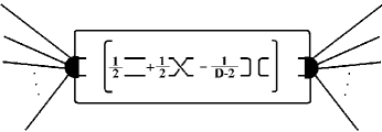
Figure 4: A graphical representation of a propagator contraction in an amplitude. The black half dots represent an arbitrary internal structure for the amplitude, the full lines between the two half dots are internal contractions of indices, the outgoing lines represents index contractions with external sources.

Essentially (disregarding symmetrizations of indices etc) only the following contractions of indices in the conventional graviton propagator can occur in an given amplitude, we can contract, e.g., ($\alpha$ and $\beta$) or both ($\alpha$ and $\beta$) and ($\gamma$ and $\delta$). The results of such contractions are shown below and also graphically depicted in figure 5.

$$\begin{split}\frac{1}{2}[\eta_{\alpha\gamma}\eta_{\beta\delta}+\eta_{\alpha\delta}\eta_{\beta\gamma}-\frac{2}{D-2}\eta_{\alpha\beta}\eta_{\gamma\delta}\Big{]}\eta^{\alpha\beta}=\eta_{\gamma\delta}-\frac{D}{D-2}\eta_{\gamma\delta}\\ \frac{1}{2}[\eta_{\alpha\gamma}\eta_{\beta\delta}+\eta_{\alpha\delta}\eta_{\beta\gamma}-\frac{2}{D-2}\eta_{\alpha\beta}\eta_{\gamma\delta}\Big{]}\eta^{\alpha\beta}\eta^{\gamma\delta}=-\frac{2D}{D-2}\end{split}$$ (14)

We can can also contract, e.g., ($\alpha$ and $\gamma$) or both ($\alpha$ and $\gamma$) and ($\beta$ and $\delta$) again the results are shown below and depicted graphically in figure 6.

$$\begin{split}\frac{1}{2}[\eta_{\alpha\gamma}\eta_{\beta\delta}+\eta_{\alpha\delta}\eta_{\beta\gamma}-\frac{2}{D-2}\eta_{\alpha\beta}\eta_{\gamma\delta}\Big{]}\eta^{\alpha\gamma}=\frac{1}{2}\eta_{\beta\delta}D+\eta_{\beta\delta}\left(\frac{1}{2}+\frac{1}{D-2}\right)\\ \frac{1}{2}[\eta_{\alpha\gamma}\eta_{\beta\delta}+\eta_{\alpha\delta}\eta_{\beta\gamma}-\frac{2}{D-2}\eta_{\alpha\beta}\eta_{\gamma\delta}\Big{]}\eta^{\alpha\gamma}\eta^{\beta\delta}=D^{2}-\frac{D}{D-2}\end{split}$$ (15)

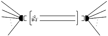
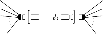
Figure 5: Two possible types of contractions for the propagator. Whenever we have an index loop we have a contraction of indices. It is seen that none of the above contractions will generate something with a positive power of ($D$).

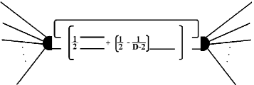
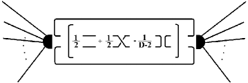
Figure 6: Two other types of index contractions for the propagator. Again it is seen that only the $(\eta_{\alpha\gamma}\eta_{\beta\delta}+\eta_{\alpha\delta}\eta_{\beta\gamma})$ part of the propagator is important in large-$D$ considerations.

As it is seen, only the $(\eta_{\alpha\gamma}\eta_{\beta\delta}+\eta_{\alpha\delta}\eta_{\beta\gamma})$ part of the propagator will have the possibility to contribute with a positive power of ($D$). Whenever the $\left(\frac{\eta_{\mu\nu}\eta_{\alpha\beta}}{D-2}\right)$ term in the propagator is in play, e.g., what remains is something that goes as $\left(\sim\frac{D}{D-2}\right)$ and which consequently will have no support to the large-$D$ leading loop contributions.

We have seen that different index structures go into the same vertex factor. Below (see figure 7), we depict the same 2-loop diagram, but for different index structures of the external 3-point vertex factor (i.e., (3C) and (3E)) for the external lines.

Figure 7: Different trace structures in the same diagram, generated by different index structures in the vertex (i.e., (3C) and (3E) respectively), the first diagram have three traces, $\sim D^{3}$, the other diagram have only two traces, $\sim D^{2}$.

Different types of trace structures will hence occur in the same loop diagram. Every diagram will consist of a sum of contributions with a varying number of traces. It is seen that the graphical depiction of the index structure in the vertex factor is a very useful tool in determining the trace structure of various diagrams.

The following type of two-point diagram (see figure 9) build from the (3B) or (3C) parts of the 3-point vertex will generate a contribution which carries a maximal number of traces compared to the number of vertices in the diagram.

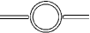
Figure 8: A diagrammatic representation of some leading contributions to the 2-point 1-loop graph in the large-$D$ limit.

Figure 9: Some non-leading contributions to the 2-point 1-loop graph in the large-$D$ limit.

The other parts of the 3-point vertex factor, e.g., the (3A) or (3E) parts respectively will not generate a leading contribution in the large-$D$ limit, however such contributions will go into the non-leading contributions of the theory (see figure 9). The diagram built from the (3A) index structure will, e.g., not carry a leading contribution due to our previous considerations regarding contractions of the indices in the propagator (see figure 5).

It is crucial that we obtain a consistent limit for the graphs, when we take ($D\rightarrow\infty$). In order to cancel the factor of ($D^{2}$) from the above type of diagrams, i.e., to put it on equal footing in powers of ($D$) as the simple propagator diagram, it is seen that we need to rescale $\left(\kappa\rightarrow\frac{\kappa}{D}\right)$. In the large-$D$ limit $\left(\frac{\kappa}{D}\right)$ will define the ’new’ redefined gravitational coupling. A finite limit for the 2-point function will be obtained by this choice, i.e, the leading $D$-contributions will not diverge, when the limit ($D\rightarrow\infty$) is imposed. By this choice all leading $n$-point diagrams will be well defined and go as $\left(\sim\left(\frac{\kappa}{D}\right)^{(n-2)}\right)$ in a $\left(\frac{1}{D}\right)$ expansion. Each external line will carry a gravitational coupling  . However, it is important to note that our rescaling of $(\kappa)$ is solely determined by the requirement of creating a finite consistent large-$D$ limit, where all $n$-point tree diagrams and their loop corrections are on an equal footing. The above rescaling seems to be the obvious to do from the viewpoint of creating a physical consistent theory. However, we note that other limits for the graphs are in fact possible by other redefinitions of $(\kappa)$ but such rescalings will, e.g., scale away the loop corrections to the tree diagrams, thus such rescalings must be seen as rather unphysical from the viewpoint of traditional quantum field theory.

For any loop with two propagators the maximal number of traces are obviously two. However, we do not know which diagrams will generate the maximal number of powers of $D$ in total. Some diagrams will have more traces than others, however because of the rescaling of $(\kappa)$ they might not carry a leading contribution after all. For example, if we look at the two graphs depicted in figure 10, they will in fact go as $\left(D^{3}\times\frac{\kappa^{4}}{D^{4}}\times D^{3}\sim\frac{1}{D}\right)$ and $\left(D^{5}\times\frac{\kappa^{8}}{D^{8}}\times D^{5}\sim\frac{1}{D^{3}}\right)$ respectively and thus not be leading contributions.

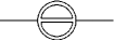
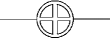
Figure 10: Two multi-loop diagrams with many traces. The rescaling of $(\kappa)$ will however render both diagrams as non-leading contributions compared to diagrams with separate loops. Here and in the next coming figures we will employ the following notation for the index structure of the lines originating from loop contributions. Whenever an line originates from a loop contribution it should be understood that there are only two possibilities for its index structure, i.e., the lines has to be of the same type as in the contracted index lines in the index structure (3B) or as the dashed lines in (3C). No assumptions on the index structures for tree external lines are made, here any viable index structures are present, but we still represent such lines with a single full line for simplicity.

In order to arrive at the result of ref. Strominger:1981jg , we have to consider the rescaling of $(\kappa)$ which will generate negative powers of $(D)$ as well. Let us now discuss the main result of ref. Strominger:1981jg .

Let ($P_{\rm\max}$) be the maximal power of ($D$) associated with a graph. Next we can look at the function ($\Pi$):

$$\Pi=2L-\sum_{m=3}^{\infty}(m-2)V_{m}.$$ (16)

Here ($L$) is the number of loops in a given diagram, and ($V_{m}$) counts the number of $m$-point vertices. It is obviously true that ($P_{\rm max}$) must be less than or equal to ($\Pi$).

The above function counts the maximal number of positive factors of ($D$) occurring for a given graph. The first part of the expression simply counts the maximal number of traces ($\sim D^{2}$) from a loop, the part which is subtracted counts the powers of ($\kappa$ $\sim\frac{1}{D}$) arising from the rescaling of ($\kappa$).

Next, we employ the two well-known formulas for the topology of diagrams:

$$L=I-V+1,$$ (17)

$$\sum_{m=3}^{\infty}mV_{m}=2I+E,$$ (18)

where ($I$) is the number of internal lines, $\left(V=\sum_{m=3}^{\infty}V_{m}\right)$ is total number of vertices and ($E$) is the number of external lines.

Putting these three formulas together one arrives at:

$$P_{\rm max}\leq 2-E-2\sum_{m=3}^{\infty}V_{m}.$$ (19)

Hence, the maximal power of ($D$) is obtained in the case of graphs with a minimal number of external lines, and two traces per diagram loop. In order to generate the maximum of two traces per loop, separated loops are necessary, because whenever a propagator index line is shared in a diagram we will not generate a maximal number of traces. Considering only separated bubble graphs, thus the following type of $n$-point (see figure 11) diagrams will be preferred in the large-$D$ limit:

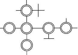
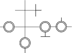
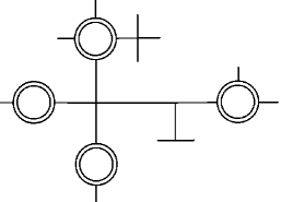
Figure 11: Examples of multi-loop diagrams with leading contributions in the large-$D$ limit.

Vertices, which generate unnecessary additional powers of $\left(\frac{1}{D}\right)$, are suppressed in the large-$D$ limit; multi-loop contributions with a minimal number of vertex lines will dominate over diagrams with more vertex lines. That is, in figure 12 the first diagram will dominate over the second one.

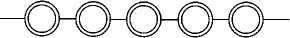
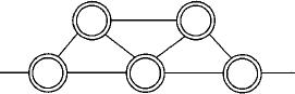
Figure 12: Of the following two diagrams with double trace loops the first one will be leading.

Thus, separated bubble diagrams will contribute to the large-$D$ limit in quantum gravity. The 2-point bubble diagram limit is shown in figure 13.

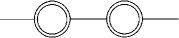
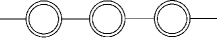
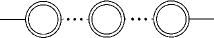
Figure 13: Leading bubble 2-point diagrams.

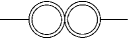
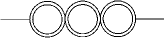
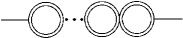
Figure 14: Another type of 2-point diagram build from the index structure (4J), which will be leading in the large-$D$ limit.

Another type of diagrams which can make leading contributions, is the diagrams depicted in figure 14. These contributions are of a type where a propagator directly combines different legs in a vertex factor with a double trace loop. Because of the index structure (4J) in the 4-point vertex such contributions are possible. These types of diagrams will have the same dimensional dependence: $\left(\frac{\kappa^{4}}{D^{4}}\times D^{4}\sim 1\right)$, as the 2-loop separated bubble diagrams. It is claimed in Strominger:1981jg , that such diagrams will be non-leading. We have however found no evidence of this in our investigations of the large-$D$ limit.

Higher order vertices with more external legs can generate multi-loop contributions of the vertex-loop type, e.g., a 6-point vertex can in principle generate a 3-loop contribution to the 3-point function, a 8-point vertex a 4-loop contribution the the 4-point function etc (see figure 15).

Figure 15: Particular examples of leading vertex-loop diagrams build from 6-point and 8-point vertex factors respectively.

The 2-point large-$D$ limit will hence consist of the sum of the propagator and all types of leading 2-point diagrams which one considered above, i.e., bubble diagrams and vertex-loops diagrams and combinations of the two types of diagrams. Ghost insertions will be suppressed in the large-$D$ limit, because such diagrams will not carry two traces, however they will go into the theory at non-leading order. The general $n$-point function will consist of diagrams built from separated bubbles or vertex-loop diagrams. We have devoted appendix B to a study of the generic $n$-point functions.

III The large-$D$ limit and the effective field theory extension of gravity

So far we have avoided the renormalization difficulties of Einstein gravity. In order to obtain a effective renormalizable theory up to the Planck scale we will have to introduce the effective field theory description.

The most general effective Lagrangian of a $D$-dimensional gravitational theory has the form:

$${\cal L}=\int d^{D}x\sqrt{-g}\bigg{(}\Big{(}\frac{2}{\kappa^{2}}R+c_{1}R^{2}+c_{2}R_{\mu\nu}R^{\mu\nu}+\ldots\Big{)}+{\cal L}_{\rm eff.\ matter}\bigg{)},$$ (20)

where ($R^{\alpha}_{\ \mu\nu\beta}$) is the curvature tensor ($g=-{\rm det}(g_{\mu\nu})$) and the gravitational coupling is defined as before, i.e., ($\kappa^{2}=32\pi G_{D}$). The matter Lagrangian includes in principle everything which couples to a gravitational field matter , i.e., any effective or higher derivative couplings of gravity to bosonic and or fermionic matter. In this paper we will however solely look at pure gravitational interactions. The effective Lagrangian for the theory is then reduced to invariants built from the Riemann tensors:

$${\cal L}=\int d^{D}x\sqrt{-g}\Big{(}\frac{2R}{\kappa^{2}}+c_{1}R^{2}+c_{2}R_{\mu\nu}R^{\mu\nu}+\ldots\Big{)}.$$ (21)

In an effective field theory higher derivative couplings of the fields are allowed for, while the underlying physical symmetries of the theory are kept manifestly intact. In gravity the general action of the theory has to be covariant with respect to the external gravitational fields.

The renormalization problems of traditional Einstein gravity are trivially solved by the effective field theory approach. The effective treatment of gravity includes all possible invariants and hence all divergences occurring in the loop diagrams can be absorbed in a renormalized effective action.

The effective expansion of the theory will be an expansion of the Lagrangian in powers of momentum, and the minimal powers of momentum will dominate the effective field theory at low energy scales. In gravity this means that the ($R\sim({\rm momentum})^{2}$) term will be dominant at normal energies, i.e., gravity as an effective field theory at normal energies will essentially still be general relativity. At higher energy scales the higher derivative terms ($R^{2}\sim({\rm momentum})^{4}),\ \ldots,(\ R^{3}\sim({\rm momentum})^{6})\ldots$, corresponding to higher powers of momentum will mix in and become increasingly important.

The large-$D$ limit in Einstein gravity is arrived at by expanding the theory in ($D$) and subsequently taking ($D\rightarrow\infty$). This can be done in its effective extension too. Treating gravity as an effective theory and deriving the large-$D$ limit results in a double expansion of the theory, i.e., we expand the theory both in powers of momentum and in powers of $\left(\frac{1}{D}\right)$. In order to understand the large-$D$ limit in the case of gravity as an effective field theory, we have to examine the vertex structure for the additional effective field theory terms. Clearly any vertex contribution from, e.g., the effective field theory terms, ($R^{2}$), and, ($R_{\mu\nu}^{2}$), will have four momentum factors and hence new index structures are possible for the effective vertices.

We find the following vertex structure for the ($R^{2}$) and the ($R_{\mu\nu}^{2}$) terms of the effective action (see figure 16 and appendix A).

$V_{3}^{\rm eff}=$	$\kappa^{3}\left(\parbox{28.45274pt}{\includegraphics[height=22.76228pt]{fig16.1.ps}}\right)^{\rm eff}_{\rm 3A}$+	$\kappa^{3}\left(\parbox{28.45274pt}{\includegraphics[height=22.76228pt]{fig16.2.ps}}\right)^{\rm eff}_{\rm 3B}$+	$\kappa^{3}\left(\parbox{28.45274pt}{\includegraphics[height=22.76228pt]{fig16.3.ps}}\right)^{\rm eff}_{\rm 3C}$+	$\kappa^{3}\left(\parbox{28.45274pt}{\includegraphics[height=22.76228pt]{fig16.4.ps}}\right)^{\rm eff}_{\rm 3D}$+	$\kappa^{3}\left(\parbox{28.45274pt}{\includegraphics[height=22.76228pt]{fig16.5.ps}}\right)^{\rm eff}_{\rm 3E}$+
	$\kappa^{3}\left(\parbox{28.45274pt}{\includegraphics[height=22.76228pt]{fig16.6.ps}}\right)^{\rm eff}_{\rm 3F}$+	$\kappa^{3}\left(\parbox{28.45274pt}{\includegraphics[height=22.76228pt]{fig16.7.ps}}\right)^{\rm eff}_{\rm 3G}$+	$\kappa^{3}\left(\parbox{28.45274pt}{\includegraphics[height=22.76228pt]{fig16.8.ps}}\right)^{\rm eff}_{\rm 3H}$+	$\kappa^{3}\left(\parbox{28.45274pt}{\includegraphics[height=22.76228pt]{fig16.9.ps}}\right)^{\rm eff}_{\rm 3I}$.

Figure 16: A graphical representation of the ($R^{2}$) and the ($R^{2}_{\mu\nu}$) index structures in the effective 3-point vertex factor. A dashed line represents a contraction of a index with a momentum line. A full line symbolizes a contraction of two index lines.

We are particularly interested in the terms which will give leading trace contributions. For the (3B)^eff and (3C)^eff index structures of we have shown some explicit results (see figure 17).

$\left(\parbox{28.45274pt}{\includegraphics[height=22.76228pt]{fig17.1.ps}}\right)^{\rm eff}_{\rm 3B}$	$\sim{\rm sym}[-P_{3}\left(\eta_{\mu\alpha}\eta_{\nu\sigma}\eta_{\beta\gamma}[3c_{1}k_{1}^{2}(k_{2}\cdot k_{3})+c_{2}(\frac{1}{2}(k_{1}\cdot k_{2})(k_{1}\cdot k_{3})-\frac{1}{4}k_{2}^{2}k_{3}^{2})]\right)$
	$-P_{6}\left(\eta_{\mu\alpha}\eta_{\nu\sigma}\eta_{\beta\gamma}[2c_{1}k_{1}^{2}k_{3}^{2}+c_{2}(\frac{1}{2}(k_{1}\cdot k_{3})^{2}-\frac{1}{4}k_{2}^{2}(k_{1}\cdot k_{3}))]\right)],$
$\left(\parbox{28.45274pt}{\includegraphics[height=22.76228pt]{fig17.2.ps}}\right)^{\rm eff}_{\rm 3C}$	$\sim{\rm sym}[-P_{3}\left(k_{1\mu}k_{1\alpha}\eta_{\nu\sigma}\eta_{\beta\gamma}[3c_{1}k_{2}\cdot k_{3}]\right)-2P_{6}\left(k_{1\mu}k_{1\alpha}\eta_{\nu\sigma}\eta_{\beta\gamma}[c_{1}k_{3}^{2}]\right)+\frac{1}{2}P_{6}\left(k_{1\mu}k_{2\alpha}\eta_{\nu\sigma}\eta_{\beta\gamma}[c_{2}k_{1}\cdot k_{3}]\right)$
	+$P_{6}\left(k_{1\mu}k_{3\alpha}\eta_{\nu\sigma}\eta_{\beta\gamma}[c_{2}k_{1}\cdot k_{3}]\right)-\frac{1}{2}P_{3}\left(k_{2\mu}k_{3\alpha}\eta_{\nu\sigma}\eta_{\beta\gamma}[c_{2}k_{1}^{2}]\right)-\frac{1}{2}P_{6}\left(k_{3\mu}k_{3\alpha}\eta_{\nu\sigma}\eta_{\beta\gamma}[c_{2}k_{1}^{2}]\right)$
	$-\frac{1}{2}P_{6}\left(k_{1\beta}k_{3\nu}\eta_{\mu\sigma}\eta_{\alpha\gamma}[c_{2}k_{2}^{2}]\right)-\frac{1}{2}P_{6}\left(k_{3\beta}k_{3\nu}\eta_{\mu\sigma}\eta_{\alpha\gamma}[c_{2}k_{2}^{2}]\right)].$

Figure 17: Explicit index structure terms in the effective vertex 3-point factor, which can contribute with leading contributions in the large-$D$ limit.

It is seen that also in the effective theory there are terms which will generate double trace structures. Hence an effective 1-loop bubble diagram with two traces is possible. Such diagrams will go as $\left(\frac{\kappa^{4}}{D^{4}}c_{1}\times D^{2}\sim\frac{c_{1}}{D^{2}}\right)$. In order to arrive at the same limit for the effective tree diagrams as the tree diagrams in Einstein gravity we need to rescale ($c_{1}$) and ($c_{2}$) by ($D^{2}$) i.e., ($c_{1}\rightarrow c_{1}D^{2}$) and ($c_{2}\rightarrow c_{2}D^{2}$). Thereby every $n$-point function involving the effective vertices will go into the $n$-point functions of Einstein gravity. In fact this will hold for any ($c_{i}$) provided that the index structures giving double traces also exists for the higher order effective terms. Other rescalings of the ($c_{i}$)’s are possible. But such other rescalings will give a different tree limit for the effective theory at large-$D$. The effective tree-level graphs will be thus be scaled away from the Einstein tree graph limit.

The above rescaling with ($c_{i}\rightarrow c_{i}D^{2}$) corresponds to the maximal rescaling possible. Any rescaling with, e.g., ($c_{i}\rightarrow c_{i}D^{n}$, $n>2$) will not be possible, if we still want to obtain a finite limit for the loop graphs at ($D\rightarrow\infty$). A rescaling with $(D^{2})$ will give maximal support to the effective terms at large-$D$.

The effective terms in the action are needed in order to renormalize infinities from the loop diagrams away. The renormalization of the effective field theory can be carried out at any particular ($D$). Of course the exact cancellation of pole terms from the loops will depend on the integrals, and the algebra will change with the dimension, but one can take this into account for any particular order of $(D=D_{p})$ by an explicit calculation of the counter terms at dimension ($D_{p}$) followed by an adjustment of the coefficients in the effective action. The exact renormalization will in this way take place order by order in $\left(\frac{1}{D}\right)$. For any rescaling of the $(c_{i})$’s it is thus always possible carry out a renormalization of the theory. Depending on how the rescaling of the coefficients $(c_{i})$ are done, there will be different large-$D$ limits for the effective field theory extension of the theory.

The effective field theory treatment does in fact not change the large-$D$ of gravity as much as one could expect. The effective enlargement of gravity does not introduce new exciting leading diagrams. Most parts of our analysis of the large-$D$ limit depends only on the index structure for the various vertices, and the new index structures provided by the effective field theory terms only add new momentum lines, which do not give additional traces over index loops. Therefore the effective extension of Einstein gravity is not a very radical change of its large-$D$ limit. In the effective extension of gravity the action is trivially renormalizable up to a cut-off scale at ($M_{\rm Planck}$) and the large-$D$ expansion just as well defined as an large-$N$ expansion of a renormalizable planar expansion of a Yang-Mills action.

As a subject for further investigations, it might be useful to employ more general considerations about the index structures. Seemingly all possible types of index-structures are present in the effective field theory extension of gravity in the conventional approach. As only certain index structures go into the leading large-$D$ limit, the ’interesting’ index structures can be classified at any given loop order. In fact one could consider loop amplitudes with only ’interesting’ index structures present. Such applications might useful in very complicated quantum gravity calculations, where only the leading large-$D$ behavior is interesting.

A comparison of the index structures present in other field expansions and the conventional expansion might also be a working area for further investigations. Every index structure in the conventional expansion of the field can be build up from the following types of index structures, see figure 18.

Figure 18: The first 8 basic index structures which builds up any conventional vertex factor.

Thus, it is not possible to consider any index structures in a 3- or 4-point vertex, which cannot be decomposed into some product of the above types of index contractions. It might be possible to extend this to something useful in the analysis of the large-$D$ limit, e.g., a simpler description of the large-$D$ diagrammatic truncation of the theory. This is another interesting working area for further research.

IV Considerations about the space-time integrals

The space-time integrals pose certain fundamental restrictions to our analysis of the large-$D$ limit in gravity. So far we have considered only the algebraic trace structures of the $n$-point diagrams. This analysis lead us to a consistent large-$D$ limit of gravity, where we saw that only bubble and vertex-loop diagrams will carry the leading contributions in $\left(\frac{1}{D}\right)$. In a large-$N$ limit of a gauge theory this would have been adequate, however the space-time dimension is much more that just a symmetry index for the gauge group, and has a deeper significance for the physical theory than just that of a symmetry index. Space-time integrations in a $D$-dimensional world will contribute extra dimensional dependencies to the graphs, and it thus has to be investigated if the $D$-dimensional integrals could upset the algebraic large-$D$ limit. The issue about the $D$-dimensional integrals is not resolved in ref. Strominger:1981jg , only explicit examples are discussed and some conjectures about the contributions from certain integrals in the graphs at large-$D$ are stated. It is clear that in the case of the 1-loop separated integrals the dimensional dependence will go as $\left(\sim\Gamma(\frac{D-1}{2})\right)$. Such a dimensional dependence can always be rescaled into an additional redefinition of $(\kappa)$, i.e., we can redefine $\left(\kappa\rightarrow\frac{\kappa}{\sqrt{C}}\right)$ where $\left(C\sim\Gamma(\frac{D-1}{2})\right)$. The dimensional dependence from both bubble graphs and vertex-loop graphs will be possible to scale away in this manner. Graphs which have a nested structure, i.e., which have shared propagator lines, will be however be suppressed in $(D)$ compared to the separated loop diagrams. Thus the rescaling of $(\kappa)$ will make the dimensional dependence of such diagrams even worse.

In the lack of rigorously proven mathematical statements, it is hard to be completely certain. But it is seen, that in the large-$D$ limit the dimensional dependencies from the integrations in $D$-dimensions will favor the same graphs as the algebraic graphs limit.

The effective extension of the gravitational action does not pose any problems in these considerations, concerning the dimensional dependencies of the integrals and the extra rescalings of $(\kappa)$. The conjectures made for the Einstein-Hilbert types of leading loop diagrams hold equally well in the effective field theory case. A rescaling of the effective coupling constants have of course to be considered in light of the additional rescaling of ($\kappa$). We will have ($c_{i}\rightarrow Cc_{i}$) in this case. Nested loop diagrams, which algebraically will be down in $\left(\frac{1}{D}\right)$ compared to the leading graphs, will also be down in $\left(\frac{1}{D}\right)$ in the case of an effective field theory.

To directly resolve the complications posed by the space-time integrals, in principle all classes of integrals going into the $n$-point functions of gravity have to be investigated. Such an investigation would indeed be a very ambitious task and it is outside the scope of this investigation. However, as a point for further investigations, this would be an interesting place to begin a more rigorous mathematical justification of the large-$D$ limit.

To avoid any complications with extra factors of ($D$) arising from the evaluation of the integrals, one possibility is to treat the extra dimensions in the theory as compactified Kaluza-Klein space-time dimensions. The extra dimensions are then only excited above the Planck scale. The space-time integration will then only have to be preformed over a finite number of space-time dimensions, e.g., the traditional first four. In such a theory the large-$D$ behavior is solely determined by the algebraic traces in the graphs and the integrals cannot not contribute with any additional factors of ($D$) to the graphs. Having a cutoff of the theory at the Planck scale is fully consistent with effective treatment of the gravitational action. The effective field theory description is anyway only valid up until the Planck scale, so an effective action having a Planckian Kaluza-Klein cutoff of the momentum integrations, is a possibility.

V Comparison of the large-$N$ limit and the large-$D$ limit

The large-$N$ limit of a gauge theory and the large-$D$ limit in gravity has some similarities and some dissimilarities which we will look upon here.

The large-$N$ limit in a gauge theory is the limit where the symmetry indices of the gauge theory can go to infinity. The idea behind the gravity large-$D$ limit is to do the same, where in this case ($D$) will play the role of ($N$), we thus treat the spatial dimension ($D$) as if it is only a symmetry index for the theory, i.e., a physical parameter, in which we are allowed to make an expansion.

As it was shown by ’t Hooft in ref. tHooft the large-$N$ limit in a gauge theory will be a planar diagram limit, consisting of all diagrams which can be pictured in a plane. The leading diagrams will be of the type depicted in figure 19.

Figure 19: A particular planar diagram in the large-$N$ limit. A $(\times)$ symbolizes an external source, the full lines are index lines, an full internal index loop gives a factor of ($N$).

The arguments for this diagrammatic limit follow similar arguments to those we applied in the large-$D$ limit of gravity. However the index loops in the gauge theory are index loops of the internal symmetry group, and for each type of vertex there will only be one index structure. Below we show the particular index structure for a 3-point vertex in a gauge theory.

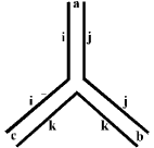
Figure 20: The index structure for the 3-point in vertex in a gauge theory.

This index structure is also present in the gravity case, i.e., in the (3E) index structure, but various other index structure are present too, e.g., (3A), (3B), $\ldots$, and each index structure will generically give dissimilar traces, i.e., dissimilar factors of ($D$) for the loops.

In gravity only certain diagrams in the large-$D$ limit carry leading contributions, but only particular parts of the graph’s amplitudes will survive when ($D\rightarrow\infty$) because of the different index structures in the vertex factor. The gravity large-$D$ limit is hence more like a truncated graph limit, where only some parts of the graph amplitude will be important, i.e., every leading graph will also carry contributions which are non-leading.

In the Yang-Mills large-$N$ limit the planar graph’s amplitudes will be equally important as a whole. No truncation of the graph’s amplitudes occur. Thus, in a Yang-Mills theory the large-$N$ amplitude is found by summing the full set of planar graphs. This is a major dissimilarity between the two expansions

The leading diagram limits in the two expansions are not identical either. The leading graphs in gravity at large-$D$ are given by the diagrams which have a possibility for having a closed double trace structure, hence the bubble and vertex-loop diagrams are favored in the large-$D$ limit. The diagrams contributing to the gravity large-$D$ limit will thus only be a subset of the full planar diagram limit.

VI Other expansions of the fields

In gravity it is a well-known fact that different definitions of the fields will lead to different results for otherwise similar diagrams. Only the full amplitudes will be gauge invariant and identical for different expansions of the gravitational field. Therefore comparing the large-$D$ diagrammatical expansion for dissimilar definitions of the gravitational field, diagram for diagram, will have no meaning. The analysis of the large-$D$ limit carried out in this paper is based on the conventional definition of the gravitational field, and the large-$D$ diagrammatic expansion should hence be discussed in this light.

Other field choices may be considered too, and their diagrammatic limits should be investigated as well. It may be worth some efforts and additional investigations to see, if the diagrammatic large-$D$ limit considered here is an unique limit for every definition of the field, i.e., to see if the same diagrammatic limit always will occur for any definition of the gravitational field. A scenario for further investigations of this, could e.g., be to look upon if the field expansions can be dressed in such a way that we reach a less complicated diagrammatic expansion at large-$D$, at the cost of having a more complicated expansion of the Lagrangian. For example, it could be that vertex-loop corrections are suppressed for some definitions of the gravitational field, but that more complicated trace structures and cancellations between diagrams occurs in the calculations. In the case of the Goldberg definition of the gravitational field the vertex index structure is less complicated Strominger:1981jg , however the trace contractions of diagrams appears to much more complicated than in the conventional method. It should be investigated more carefully if the Goldberg definition of the field may be easier to employ in calculations. Indeed the diagrammatical limit considered by Strominger:1981jg is easier, but it is not clear if results from two different expansions of the gravitational field are used to derive this. Further investigations should sheet more light on the large-$D$ limit, and on how a field redefinition may or may not change its large-$D$ diagrammatic expansion.

Furthermore one can consider the background field method in the context of the large-$D$ limit as well. This is another working area for further investigations. The background field method is very efficient in complicated calculations and it may be useful to employ it in the large-$D$ analysis of gravity as well. No problems in using background field methods together with a large-$D$ quantum gravity expansion seems to be present.

VII Discussion

In this paper we have discussed the large-$D$ limit of effective quantum gravity. In the large-$D$ limit, a particular subset of planar diagrams will carry all leading $\left(\frac{1}{D}\right)$ contributions to the $n$-point functions. The large-$D$ limit for any given $n$-point function will consist of the full tree $n$-point amplitude, together with a set of loop corrections which will consist of the leading bubble and vertex-loop graphs we have considered. The effective treatment of the gravitational action insures that a renormalization of the action is possible and that none of the $n$-point renormalized amplitudes will carry uncancelled divergent pole terms. An effective renormalization of the theory can be preformed at any particular dimensionality.

The leading $\left(\frac{1}{D}\right)$ contributions to the theory will be algebraically less complex than the graphs in the full amplitude. Calculating only the $\left(\frac{1}{D}\right)$ leading contributions simplifies explicit calculations of graphs in the large-$D$ limit. The large-$D$ limit we have found is completely well defined as long as we do not extend the space-time integrations to the full $D$-dimensional space-time. That is, we will always have a consistent large-$D$ theory as long as the integrations only gain support in a finite dimensional space-time and the remaining extra dimensions in the space-time is left as compactified, e.g., below the Planck scale.

We hence have a renormalizable, definite and consistent large-$D$ limit for effective quantum gravity – good below the Planck scale!

No solution to the problem of extending the space-time integrals to a full $D$-dimensional space-time has been presented in this paper, however it is clear that the effective treatment of gravity do not impose any additional problems in such investigations. The considerations about the $D$-dimensional integrals discussed in ref. Strominger:1981jg hold equally well in a effective field theory, however as well as we will have to make an additional rescaling of ($\kappa$) in order to account for the extra dimensional dependence coming from the $D$-dimensional integrals, we will have make an extra rescaling of the coefficients ($c_{i}$) in the effective Lagrangian too.

Our large-$D$ graph limit is not in agreement with the large-$D$ limit of ref. Strominger:1981jg , the bubble graph are present in both limits, but vertex-loops are not allowed and claimed to be down in $\left(\frac{1}{D}\right)$ the latter. We do not agree on this point, and believe that this might be a consequence of comparing similar diagrams with different field definitions. It is a well-known fact in gravity that dissimilar field definitions lead to different results for the individual diagrams. Full amplitudes are of course unaffected by any particular definition of the field, but results for similar diagrams with different field choices cannot be immediately compared.

Possible extensions of the large-$D$ considerations discussed here would be to allow for external matter in the Lagrangian. This might present some new interesting aspects in the analysis, and would relate the theory more directly to external physical observables, e.g., scattering amplitudes, and corrections to the Newton potential at large-$D$ or to geometrical objects such as a space-time metric. The investigations carried out in B1 ; B2 could be discussed from a large-$D$ point of view.

Investigations in quantum gravitational cosmology may also present an interesting work area for applications of the large-$D$ limit, e.g. quantum gravity large-$D$ big bang models etc.

The analysis of the large-$D$ limit in quantum gravity have prevailed that using the physical dimension as an expansion parameter for the theory, is not as uncomplicated as expanding a Yang-Mills theory at large-$N$. The physical dimension goes into so many aspects of the theory, e.g., the integrals, the physical interpretations etc, that it is far more complicated to understand a large-$D$ expansion in gravity than a large-$N$ expansion in a Yang-Mills theory. In some sense it is hard to tell what the large-$D$ limit of gravity really physically relates to, i.e., what describes a gravitational theory with infinitely many spatial dimensions? One way to look at the large-$D$ limit in gravity, might be to see the large-$D$ as a physical phase transition of the theory at the Planck scale. This suggests that the large-$D$ expansion of gravity should be seen as a very high energy scale limit for a gravitational theory.

Large-$N$ expansions of gauge theories tHooft have many interesting calculational and fundamental applications in, e.g., string theory, high energy, nuclear and condensed matter physics. A planar diagram limit for a gauge theory will be a string theory at large distance, this can be implemented in relating different physical limits of gauge theory and fundamental strings. In explicit calculations, large-$N$ considerations have many important applications, e.g., in the approximation of QCD amplitudes from planar diagram considerations or in the theory of phase-transitions in condensed matter physics, e.g., in theories of superconductivity, where the number of particles will play the role of ($N$).

High energy physics and string theory are not the only places where large symmetry investigations can be employed to obtain useful information. As a calculational tool large-$D$ considerations can be imposed in quantum mechanics to obtain useful information about eigenvalues and wave-functions of arbitrary quantum mechanical potentials with a extremely high precision Bjerrum-Bohr:qr .

Practical applications of the large-$D$ limit in explicit calculations of $n$-point functions could be the scope for further investigations as well as certain limits of string theory might be related to the large-$D$ limit in quantum gravity. The planar large-$D$ limit found in our investigation might resemble that of a truncated string limit at large distances? Investigations of the (Kawai-Lewellen-Tye KLT ) open/closed string, gauge theory/gravity relations could also be interesting to preform in the context of a large-$D$ expansion. (See e.g., Bern3 ; Bern:2002kj ; BjerrumBohr:2003af ; Bjerrum-Bohr:2003vy for resent work on this subject. See also  Deser:1998jz ; Deser:2000xz ) Such questions are outside the scope of this investigation, however knowing the huge importance of large-$N$ considerations in modern physics, large-$D$ considerations of gravity might pose very interesting tasks for further research.

Appendix A Effective 3- and 4-point vertices

The effective Lagrangian takes the form:

$${\cal L}=\int d^{D}x\sqrt{-g}\Big{(}\frac{2R}{\kappa^{2}}+c_{1}R^{2}+c_{2}R_{\mu\nu}R^{\mu\nu}+\ldots\Big{)}.$$ (22)

In order to find the effective vertex factors we need to expand $(\sqrt{-g}R^{2})$ and $(\sqrt{-g}R_{\mu\nu}^{2})$.

We are working in the conventional expansion of the field, so we define:

$$g_{\mu\nu}\equiv\eta_{\mu\nu}+\kappa h_{\mu\nu}.$$ (23)

To second order we find the following expansion for ($\sqrt{-g}$):

$$\sqrt{-g}=\exp\left(\frac{1}{2}\log(\eta_{\mu\nu}+\kappa h_{\mu\nu})\right)=\left(1+\frac{\kappa}{2}h_{\alpha}^{\alpha}-\frac{\kappa^{2}}{4}h_{\alpha}^{\beta}h^{\alpha}_{\beta}+\frac{\kappa^{2}}{8}(h_{\alpha}^{\alpha})^{2}\ldots\right).$$ (24)

To first order in ($\kappa$) we have the following expansion for ($R$):

$$\begin{split}R^{(1)}=\kappa\left[\partial_{\alpha}\partial^{\alpha}h_{\beta}^{\beta}-\partial^{\alpha}\partial^{\beta}h_{\alpha\beta}\right],\end{split}$$ (25)

and to second order in ($\kappa^{2}$) we find:

$$\begin{split}R^{(2)}&=\kappa^{2}\Big{[}-\frac{1}{2}\partial_{\alpha}\left[h_{\mu}^{\beta}\partial^{\alpha}h_{\beta}^{\mu}\right]+\frac{1}{2}\partial_{\beta}\left[h_{\nu}^{\beta}(2\partial_{\alpha}h^{\nu\alpha}-\partial_{\nu}h_{\alpha}^{\alpha})\right]+\frac{1}{4}\left[\partial_{\alpha}h_{\beta}^{\nu}+\partial_{\beta}h_{\alpha}^{\nu}-\partial^{\nu}h_{\beta\alpha}\right]\left[\partial^{\alpha}h_{\nu}^{\beta}+\partial_{\nu}h^{\beta\alpha}-\partial^{\beta}h_{\nu}^{\alpha}\right]\\ &-\frac{1}{4}\left[2\partial_{\alpha}h^{\nu\alpha}-\partial^{\nu}h_{\alpha}^{\alpha}\right]\partial_{\nu}h_{\beta}^{\beta}-\frac{1}{2}h^{\nu\alpha}\partial_{\nu}\partial_{\alpha}h^{\beta}_{\beta}+\frac{1}{2}h_{\alpha}^{\nu}\partial_{\beta}\left[\partial^{\alpha}h_{\nu}^{\beta}+\partial_{\nu}h^{\beta\alpha}-\partial^{\beta}h_{\nu}^{\alpha}\right]\Big{]}\end{split}$$ (26)

In the same way we find for ($R_{\mu\nu}$):

$$\begin{split}R^{(1)}_{\nu\alpha}=\frac{\kappa}{2}\left[\partial_{\nu}\partial_{\alpha}h_{\beta}^{\beta}-\partial_{\beta}\partial_{\alpha}h_{\nu}^{\beta}-\partial_{\beta}\partial_{\nu}h_{\alpha}^{\beta}+\partial^{2}h_{\nu\alpha}\right],\end{split}$$ (27)

and

$$\begin{split}R^{(2)}_{\nu\alpha}&=\kappa^{2}\Big{[}-\frac{1}{2}\partial_{\alpha}\left[h^{\beta\lambda}\partial_{\nu}h_{\lambda\beta}\right]+\frac{1}{2}\partial_{\beta}\left[h^{\beta\lambda}(\partial_{\nu}h_{\lambda\alpha}+\partial_{\alpha}h_{\nu\lambda}-\partial_{\lambda}h_{\nu\alpha})\right]\\ &+\frac{1}{4}\left[\partial_{\beta}h_{\nu}^{\lambda}+\partial_{\nu}h_{\beta}^{\lambda}-\partial^{\lambda}h_{\nu\beta}\right]\left[\partial^{\lambda}h^{\beta}_{\alpha}+\partial_{\alpha}h^{\beta}_{\lambda}-\partial^{\beta}h_{\nu\alpha}\right]-\frac{1}{4}\left[\partial_{\alpha}h_{\nu}^{\lambda}+\partial_{\nu}h_{\alpha}^{\lambda}-\partial^{\lambda}_{\alpha\nu}\right]\partial_{\lambda}h^{\beta}_{\beta}\Big{]}.\end{split}$$ (28)

From these equations we can expand to find ($R^{2}$) and ($R^{2}_{\mu\nu}$).

Formally we can write:

$$\begin{split}\sqrt{-g}R^{2}&=\frac{1}{2}h_{\alpha}^{\alpha}R^{(1)}R^{(1)}+2R^{(1)}R^{(2)}\\ &=\frac{\kappa^{3}}{2}h_{\gamma}^{\gamma}\Big{[}\partial_{\alpha}\partial^{\alpha}h_{\beta}^{\beta}-\partial^{\alpha}\partial^{\beta}h_{\alpha\beta}\Big{]}\Big{[}\partial_{\sigma}\partial^{\sigma}h_{\rho}^{\rho}-\partial^{\sigma}\partial^{\rho}h_{\sigma\rho}\Big{]}+2\kappa^{3}\Big{[}\partial_{\sigma}\partial^{\sigma}h_{\rho}^{\rho}-\partial^{\sigma}\partial^{\rho}h_{\sigma\rho}\Big{]}\bigg{[}-\frac{1}{2}\partial_{\alpha}\left[h_{\mu}^{\beta}\partial^{\alpha}h_{\beta}^{\mu}\right]\\ &+\frac{1}{2}\partial_{\beta}\left[h_{\nu}^{\beta}(2\partial_{\alpha}h^{\nu\alpha}-\partial_{\nu}h_{\alpha}^{\alpha})\right]+\frac{1}{4}\left[\partial_{\alpha}h_{\beta}^{\nu}+\partial_{\beta}h_{\alpha}^{\nu}-\partial^{\nu}h_{\beta\alpha}\right]\left[\partial^{\alpha}h_{\nu}^{\beta}+\partial_{\nu}h^{\beta\alpha}-\partial^{\beta}h_{\nu}^{\alpha}\right]\\ &-\frac{1}{4}\left[2\partial_{\alpha}h^{\nu\alpha}-\partial^{\nu}h_{\alpha}^{\alpha}\right]\partial_{\nu}h_{\beta}^{\beta}-\frac{1}{2}h^{\nu\alpha}\partial_{\nu}\partial_{\alpha}h^{\beta}_{\beta}+\frac{1}{2}h_{\alpha}^{\nu}\partial_{\beta}\left[\partial^{\alpha}h_{\nu}^{\beta}+\partial_{\nu}h^{\beta\alpha}-\partial^{\beta}h_{\nu}^{\alpha}\right]\bigg{]},\end{split}$$ (29)

and

$$\begin{split}\sqrt{-g}R^{2}_{\mu\nu}&=\frac{1}{2}h_{\gamma}^{\gamma}R_{\mu\nu}^{(1)}R^{(1)\mu\nu}-2h^{\alpha\beta}R_{\mu\alpha}^{(1)}R^{(1)\mu}_{\beta}+2R_{\mu\nu}^{(1)}R^{(2)\mu\nu}\\ &=\frac{\kappa^{3}}{8}h_{\gamma}^{\gamma}\Big{[}\partial_{\nu}\partial_{\alpha}h_{\beta}^{\beta}-\partial_{\beta}\partial_{\alpha}h_{\nu}^{\beta}-\partial_{\beta}\partial_{\nu}h_{\alpha}^{\beta}+\partial^{2}h_{\nu\alpha}\Big{]}\Big{[}\partial^{\nu}\partial^{\alpha}h_{\rho}^{\rho}-\partial_{\rho}\partial^{\alpha}h^{\nu\rho}-\partial_{\rho}\partial^{\nu}h^{\alpha\rho}+\partial^{2}h^{\nu\alpha}\Big{]}\\ &-\frac{\kappa^{3}}{2}h^{\rho\sigma}\Big{[}\partial_{\mu}\partial_{\sigma}h_{\gamma}^{\gamma}-\partial_{\gamma}\partial_{\sigma}h_{\mu}^{\gamma}-\partial_{\gamma}\partial_{\mu}h_{\sigma}^{\gamma}+\partial^{2}h_{\mu\sigma}\Big{]}\Big{[}\partial^{\mu}\partial_{\rho}h_{\beta}^{\beta}-\partial_{\beta}\partial_{\rho}h^{\mu\beta}-\partial_{\beta}\partial^{\mu}h_{\rho}^{\beta}+\partial^{2}h^{\mu}_{\rho}\Big{]}\\ &+\kappa^{3}\Big{[}\partial_{\nu}\partial_{\alpha}h_{\gamma}^{\gamma}-\partial_{\gamma}\partial_{\alpha}h_{\nu}^{\gamma}-\partial_{\gamma}\partial_{\nu}h_{\alpha}^{\gamma}+\partial^{2}h_{\nu\alpha}\Big{]}\Big{[}-\frac{1}{2}\partial^{\alpha}\left[h^{\beta\lambda}\partial^{\nu}h_{\lambda\beta}\right]+\frac{1}{2}\partial_{\beta}\left[h^{\beta\lambda}(\partial^{\nu}h_{\lambda}^{\alpha}+\partial^{\alpha}h^{\nu}_{\lambda}-\partial_{\lambda}h^{\nu\alpha})\right]\\ &+\frac{1}{4}\Big{[}\partial_{\beta}h^{\nu\lambda}+\partial^{\nu}h_{\beta}^{\lambda}-\partial^{\lambda}h^{\nu}_{\beta}\Big{]}\left[\partial_{\lambda}h^{\beta\alpha}+\partial^{\alpha}h^{\beta}_{\lambda}-\partial^{\beta}h^{\alpha}_{\lambda}\right]-\frac{1}{4}\left[\partial^{\alpha}h^{\nu\lambda}+\partial^{\nu}h^{\alpha\lambda}-\partial^{\lambda}h^{\alpha\nu}\right]\partial_{\lambda}h^{\beta}_{\beta}\Big{]}.\end{split}$$ (30)

Contracting only on terms which go into the $(3B)^{\rm eff}$ and $(3C)^{\rm eff}$ index structures, and putting ($\kappa=1$) for simplicity, we have found for the ($R^{2}$) contribution:

$$(R^{2})_{(3B)^{\rm eff}}=\partial^{2}h^{\rho}_{\rho}\Big{(}-\frac{3}{2}\partial_{\alpha}h^{\beta}_{\mu}\partial^{\alpha}h_{\beta}^{\mu}-2h_{\beta}^{\mu}\partial^{2}h^{\beta}_{\mu}\Big{)},$$ (31)

and

$$(R^{2})_{(3C)^{\rm eff}}=-\partial^{\sigma}\partial^{\rho}h_{\sigma\rho}\Big{(}-\frac{3}{2}\partial_{\alpha}h^{\beta}_{\mu}\partial^{\alpha}h_{\beta}^{\mu}-2h_{\beta}^{\mu}\partial^{2}h^{\beta}_{\mu}\Big{)},$$ (32)

For the ($R^{2}_{\mu\nu}$) contribution we have found:

$$(R^{2}_{\mu\nu})_{(3B)^{\rm eff}}=\frac{1}{8}h_{\gamma}^{\gamma}\partial^{2}h_{\nu\alpha}\partial^{2}h^{\nu\alpha}-\frac{1}{4}\partial_{\lambda}\partial_{\beta}h_{\gamma}^{\gamma}\partial^{\beta}h^{\nu\alpha}\partial^{\lambda}h_{\nu\alpha}-\frac{1}{2}\partial_{\lambda}\partial_{\beta}h_{\gamma}^{\gamma}h^{\nu\alpha}\partial^{\beta}\partial^{\lambda}h_{\nu\alpha}+\frac{1}{4}\partial_{\lambda}h_{\gamma}^{\gamma}\partial^{2}h_{\nu\alpha}\partial^{\lambda}h^{\nu\alpha},$$ (33)

and

$$\begin{split}(R^{2}_{\mu\nu})_{(3C)^{\rm eff}}&=\frac{1}{2}\partial_{\lambda}\partial_{\beta}h^{\lambda}_{\sigma}\partial^{\sigma}h^{\nu\alpha}\partial^{\beta}h_{\nu\alpha}+\partial_{\lambda}\partial_{\beta}h_{\sigma}^{\lambda}h^{\nu\alpha}\partial^{\sigma}\partial^{\beta}h_{\nu\alpha}-\frac{1}{4}\partial^{2}h_{\lambda\beta}\partial^{\lambda}h^{\nu\alpha}\partial^{\beta}h_{\nu\alpha}-\frac{1}{2}\partial^{2}h_{\lambda\beta}h^{\nu\alpha}\partial^{\lambda}\partial^{\beta}h_{\nu\alpha}\\ &-\frac{1}{2}\partial_{\beta}h^{\beta\lambda}\partial^{2}h_{\nu\alpha}\partial_{\lambda}h^{\nu\alpha}-\frac{1}{2}h^{\beta\lambda}\partial^{2}h_{\nu\alpha}\partial_{\lambda}\partial_{\beta}h^{\nu\alpha}.\end{split}$$ (34)

This leads to the following results for the (3B) and (3C) terms:

$\left(\parbox{28.45274pt}{\includegraphics[height=22.76228pt]{fig16.2.ps}}\right)^{\rm eff}_{\rm 3B}$	$\sim{\rm sym}[-P_{3}\left(\eta_{\mu\alpha}\eta_{\nu\sigma}\eta_{\beta\gamma}[3c_{1}k_{1}^{2}(k_{2}\cdot k_{3})+c_{2}(\frac{1}{2}(k_{1}\cdot k_{2})(k_{1}\cdot k_{3})-\frac{1}{4}k_{2}^{2}k_{3}^{2})]\right)$
	$-P_{6}\left(\eta_{\mu\alpha}\eta_{\nu\sigma}\eta_{\beta\gamma}[2c_{1}k_{1}^{2}k_{3}^{2}+c_{2}(\frac{1}{2}(k_{1}\cdot k_{3})^{2}-\frac{1}{4}k_{2}^{2}(k_{1}\cdot k_{3}))]\right)],$
$\left(\parbox{28.45274pt}{\includegraphics[height=22.76228pt]{fig16.3.ps}}\right)^{\rm eff}_{\rm 3C}$	$\sim{\rm sym}[-P_{3}\left(k_{1\mu}k_{1\alpha}\eta_{\nu\sigma}\eta_{\beta\gamma}[3c_{1}k_{2}\cdot k_{3}]\right)-2P_{6}\left(k_{1\mu}k_{1\alpha}\eta_{\nu\sigma}\eta_{\beta\gamma}[c_{1}k_{3}^{2}]\right)+\frac{1}{2}P_{6}\left(k_{1\mu}k_{2\alpha}\eta_{\nu\sigma}\eta_{\beta\gamma}[c_{2}k_{1}\cdot k_{3}]\right)$
	+$P_{6}\left(k_{1\mu}k_{3\alpha}\eta_{\nu\sigma}\eta_{\beta\gamma}[c_{2}k_{1}\cdot k_{3}]\right)-\frac{1}{2}P_{3}\left(k_{2\mu}k_{3\alpha}\eta_{\nu\sigma}\eta_{\beta\gamma}[c_{2}k_{1}^{2}]\right)-\frac{1}{2}P_{6}\left(k_{3\mu}k_{3\alpha}\eta_{\nu\sigma}\eta_{\beta\gamma}[c_{2}k_{1}^{2}]\right)$
	$-\frac{1}{2}P_{6}\left(k_{1\beta}k_{3\nu}\eta_{\mu\sigma}\eta_{\alpha\gamma}[c_{2}k_{2}^{2}]\right)-\frac{1}{2}P_{6}\left(k_{3\beta}k_{3\nu}\eta_{\mu\sigma}\eta_{\alpha\gamma}[c_{2}k_{2}^{2}]\right)].$

Using the same procedure, we can find expression for non-leading effective contributions, however this will have no implications for the loop contributions. We have only calculated 3-point effective vertex index structures in this appendix, 4-point index structures are tractable too by the same methods, but the algebra gets much more complicated in this case.

Appendix B Comments on general $n$-point functions

In the large-$D$ limit only certain graphs will give leading contributions to the $n$-point functions. The diagrams favored in the large-$D$ will have a simpler structure than the full $n$-point graphs. Calculations which would be too complicated to do in a full graph limit, might be tractable in the large-$D$ regime.

The $n$-point contributions in the large-$D$ limit are possible to employ in approximations of $n$-point functions at any finite dimension, exactly as the $n$-point planar diagrams in gauge theories can be used, e.g., at ($N=3$), to approximate $n$-point functions. Knowing the full $n$-point limit is hence very useful in the course of practical approximations of generic $n$-point functions at finite ($D$). This appendix will be devoted to the study of what is needed in order calculate $n$-point functions in the large-$D$ limit.

In the large-$D$ limit the leading 1-loop $n$-point diagrams will be of the type, as displayed in figure 21.

Figure 21: The leading 1-loop $n$-point diagram, the index structure for the external lines is not decided, they can have the momentum structure, (i.e., as in (3C)), or they can be of the contracted type, (i.e., as in (3B)). External lines can of course also originate from 4-point vertex or a higher vertex index structure such as, e.g., the index structures (4D) or (4E). This possibility will however not affect the arguments in this appendix, so we will leave this as a technical issue to be dealt with in explicit calculations of $n$-point functions.

The completely generic $n$-point 1-loop correction will have the diagrammatic expression, as shown in figure 22.

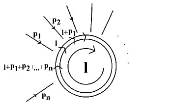
Figure 22: A diagrammatic expression for the generic $n$-point 1-loop correction.

More generically the large-$D$, $N$-loop corrections to the $n$-point function will consist of combinations of leading bubble and vertex-loop contributions, such as shown in figure 23.

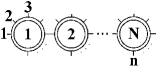
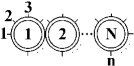
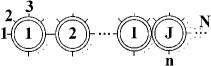
Figure 23: Some generic examples of graphs with leading contributions in the gravity large-$D$ limit. The external lines originating from a loop can only have two leading index structures, (i.e., they can be of the same type as the external lines originating from a (3B) or a (3C)) loop contribution. Tree external lines are not restricted to any particular structure, here the full vertex factor will contribute.

For the bubble contributions it is seen that all loops are completely separated. Therefore everything is known once the 1-loop contributions are calculated. That is, in order to derive the full $n$-point sole bubble contribution it is seen that if we know all $j$-point tree graphs, as well as all $i$-point 1-loop graphs (where, $i,j\leq n$) are known, the derivation the full bubble contribution is a matter of contractions of diagrams and combinatorics.

For the vertex-loop combinations the structure of the contributions are a bit more complicated to analyze. The loops will in this case be connected through the vertices, not via propagators, and the integrals can therefore be joined together by contractions of the their loop momenta. However, this does in fact not matter; we can still do the diagrams if we know all integrals which occurs in the generic 1-loop $n$-point function. The integrals in the vertex-loop diagrams will namely be of completely the same type as the bubble diagram integrals. There will be no shared propagator lines which will combine the denominators of the integrals. The algebraic contractions of indices will however be more complicated to do for vertex-loop diagrams than for sole bubble loop diagrams. Multiple index contractions from products of various integrals will have to be carried out in order to do these types of diagrams.

Computer algebraic manipulations can be employed to do the algebra in the diagrams, so we will not focus on that here. The real problem lays in the mathematical problem calculating generic $n$-point integrals.

In the Einstein-Hilbert case, where each vertex can add only two powers of momentum, we see that problem of this diagram is about doing integrals such as:

$$\begin{split}I_{n}^{(\mu_{1}\nu_{1}\mu_{2}\nu_{2}\cdots\mu_{n}\nu_{n})}=\int d^{D}l\frac{l^{\mu_{1}}l^{\nu_{1}}l^{\mu_{2}}l^{\nu_{2}}\cdots l^{\mu_{n}}l^{\nu_{n}}}{l^{2}(l+p_{1})^{2}(l+p_{1}+p_{2})^{2}\cdots(l+p_{1}+p_{2}+\ldots p_{n})^{2}},\end{split}$$ (35)

$$\begin{split}I_{n}^{(\nu_{1}\mu_{2}\nu_{2}\cdots\mu_{n}\nu_{n})}=\int d^{D}l\frac{l^{\nu_{1}}l^{\mu_{2}}l^{\nu_{2}}\cdots l^{\mu_{n}}l^{\nu_{n}}}{l^{2}(l+p_{1})^{2}(l+p_{1}+p_{2})^{2}\cdots(l+p_{1}+p_{2}+\ldots p_{n})^{2}},\end{split}$$ (36)

$$\vdots$$

$$\begin{split}I_{n}=\int d^{D}l\frac{1}{l^{2}(l+p_{1})^{2}(l+p_{1}+p_{2})^{2}\cdots(l+p_{1}+p_{2}+\ldots p_{n})^{2}},\end{split}$$ (37)

Because the graviton is a massless particle such integrals will be rather badly defined. The denominators in the integrals are close to zero, and this makes the integrals divergent. One way to deal with these integrals is to use the following parametrization of the propagator:

$$1/q^{2}=\int^{\infty}_{0}dx\exp(-xq^{2}),{\rm for}\ \ \ q^{2}>0,$$ (38)

and define the momentum integral over a complex $(2w)$-dimensional Euclidian space-time. Thus, what is left to do is gaussian integrals in a $(2w)$-dimensional complex space-time. Methods to do such types of integrals are investigated in Capper:vb ; Leibbrandt:1975dj ; Capper:pv ; Capper:dp . The results for: ($I_{2}$), ($I_{2}^{(\mu)}$), ($I_{2}^{(\mu\nu)}$) and ($I_{3}$) are in fact explicitly stated there. It is outside our scope to actually delve into technicalities about explicit mathematical manipulations of integrals, but it should be clear that mathematical methods to deal with the 1-loop $n$-point integral types exist and that this could an working area for further research. Effective field theory will add more derivatives to the loops, thus the nominator will carry additional momentum contributions. Additional integrals will hence have to be carried out in order to do explicit diagrams in an effective field theory framework.

References

- (1) G. ’t Hooft and M. J. Veltman, Annales Poincare Phys. Theor. A 20 (1974) 69.
- (2) M. H. Goroff and A. Sagnotti, Nucl. Phys. B 266 (1986) 709; A. E. van de Ven, Nucl. Phys. B 378 (1992) 309.
- (3) S. Deser and P. van Nieuwenhuizen, Phys. Rev. D 10 (1974) 401; S. Deser and P. van Nieuwenhuizen, Phys. Rev. D 10 (1974) 411; S. Deser, H. S. Tsao and P. van Nieuwenhuizen, Phys. Rev. D 10 (1974) 3337.
- (4) S. Weinberg, PhysicaA 96 (1979) 327.
- (5) J. F. Donoghue, Phys. Rev. D 50 (1994) 3874 [arXiv:gr-qc/9405057].
- (6) N. E. J. Bjerrum-Bohr, J. F. Donoghue and B. R. Holstein, Phys. Rev. D 68, 084005 (2003) [arXiv:hep-th/0211071].
- (7) N. E. J. Bjerrum-Bohr, J. F. Donoghue and B. R. Holstein, Phys. Rev. D 67, 084033 (2003) [arXiv:hep-th/0211072].
- (8) J. F. Donoghue, B. R. Holstein, B. Garbrecht and T. Konstandin, Phys. Lett. B 529, 132 (2002) [arXiv:hep-th/0112237].
- (9) N. E. J. Bjerrum-Bohr, Phys. Rev. D 66 (2002) 084023 [arXiv:hep-th/0206236].
- (10) K. S. Stelle, Gen. Rel. Grav. 9 (1978) 353.
- (11) J. Z. Simon, Phys. Rev. D 41 (1990) 3720.
- (12) A. Strominger, Phys. Rev. D 24, 3082 (1981).
- (13) G. ’t Hooft, Nucl. Phys. B 72, 461 (1974).
- (14) B.S. De Witt, Phys. Rev., Vol. 160, No. 5, 1113, 1967; B.S. De Witt, Phys. Rev., Vol. 162, No. 5, 1195, 1967; B.S. De Witt, Phys. Rev., Vol. 162, No. 5, 1239, 1967.
- (15) S. Sannan, Phys. Rev. D 34, 1749 (1986).
- (16) D. M. Capper, G. Leibbrandt and M. Ramon Medrano, Phys. Rev. D 8 (1973) 4320.
- (17) N. E. J. Bjerrum-Bohr, J. Math. Phys. 41 (2000) 2515 [arXiv:quant-ph/0302107].
- (18) H. Kawai, D. C. Lewellen and S. H. Tye, Nucl. Phys. B 269 (1986) 1.
- (19) Z. Bern and A. K. Grant, Phys. Lett. B 457 (1999) 23 [arXiv:hep-th/9904026].
- (20) Z. Bern, Living Rev. Rel. 5, 5 (2002) [arXiv:gr-qc/0206071].
- (21) N. E. J. Bjerrum-Bohr, Phys. Lett. B 560, 98 (2003) [arXiv:hep-th/0302131].
- (22) N. E. J. Bjerrum Bohr, Nucl. Phys. B 673, 41 (2003) [arXiv:hep-th/0305062].
- (23) S. Deser and D. Seminara, Phys. Rev. Lett. 82, 2435 (1999) [arXiv:hep-th/9812136].
- (24) S. Deser and D. Seminara, Phys. Rev. D 62, 084010 (2000) [arXiv:hep-th/0002241].
- (25) D. M. Capper and M. R. Medrano, Phys. Rev. D 9 (1974) 1641.
- (26) G. Leibbrandt, Rev. Mod. Phys. 47, 849 (1975).
- (27) D. M. Capper and G. Leibbrandt, J. Math. Phys. 15, 795 (1974).