hep-th/0310259

Small Black Holes on Cylinders

Troels Harmark

The Niels Bohr Institute

Blegdamsvej 17, 2100 Copenhagen Ø, Denmark

harmark@nbi.dk

Abstract

We find the metric of small black holes on cylinders, i.e. neutral and static black holes with a small mass in $d$-dimensional Minkowski-space times a circle. The metric is found using an ansatz for black holes on cylinders proposed in hep-th/0204047. We use the new metric to compute corrections to the thermodynamics which is seen to deviate from that of the $(d+1)$-dimensional Schwarzschild black hole. Moreover, we compute the leading correction to the relative binding energy which is found to be non-zero. We discuss the consequences of these results for the general understanding of black holes and we connect the results to the phase structure of black holes and strings on cylinders.

1 Introduction

Neutral and static black holes on cylinders $\mathbb{R}^{d-1}\times S^{1}$ have a more interesting dynamics and richer phase structure than black holes on flat space $\mathbb{R}^{d}$. Neutral and static black holes in flat space are for a given mass $M$ uniquely described by the Schwarzschild solution with mass $M$. With black holes on cylinders we can form a dimensionless quantity since the radius of the cylinder gives us an extra macroscopic scale in the system. This means that the behavior of the black holes can depend highly on the value of such a dimensionless quantity. This ties together with the fact that the cylinder $\mathbb{R}^{d-1}\times S^{1}$ has a non-trivial topology since it has a non-contractible cycle. This makes it possible for the black hole to grow so big that its event horizon can “meet itself” across the cylinder. It moreover makes it possible to have other types of black objects like for example black strings which have an event horizon that wrap across the cylinder.

That the phase structure of black holes on cylinders are richer than for example the Schwarzschild black holes can also be tributed to the fact that the cylinder space-time $\mathcal{M}^{d}\times S^{1}$ is not maximally symmetric unlike the Minkowski, de-Sitter and Anti-de-Sitter space-times. Until now, black hole solutions have only been found for maximally symmetric space-times or for other highly symmetric space-times. In particular solutions describing black holes on $\mathbb{R}^{2}\times S^{1}$ have been found [1, 2, 3, 4] using the Israel-Khan solution [5]. However, the $\mathbb{R}^{2}\times S^{1}$ cylinder is very different from the $\mathbb{R}^{d-1}\times S^{1}$ cylinders for $d\geq 4$ since for the $\mathcal{M}^{3}\times S^{1}$ space-time there are enough killing vectors to find the solution using the construction of Weyl [6]. For $\mathcal{M}^{d}\times S^{1}$ with $d\geq 4$ there are instead too few killing vectors to find a Weyl solution [7] which also is reflected in the fact that the metric for black holes on such cylinders does not belong to an algebraically special class [8].

The rich phase structure for black objects on cylinders have been explored from many points of view. Gregory and Laflamme [9, 10] discovered that uniform black strings on cylinders, i.e. strings that are wrapped symmetrically around the cylinder, are unstable to linear perturbations when the mass of the string is below a certain critical mass. This was interpreted to mean that a light uniform black string decays to a black hole on a cylinder since that has higher entropy. However, Horowitz and Maeda [11] argued that this transition should have an intermediate step in the form of a light non-uniform black string. Such a non-uniform string branch have not been found, but a new branch of non-uniform strings have been found by [12, 13, 14]. This new branch of non-uniform strings seemingly does not exists for the mass range when the uniform string is classically unstable.

Several proposals for the phase structure of black objects on cylinders have been put forward [11, 13, 15, 16, 17, 18, 19, 20, 21, 22, 23, 24, 25]. In [21, 22] a new phase diagram, the $(M,n)$ phase diagram, was proposed as a tool to understand the phase structure of black objects on cylinders. A similar proposal for a phase diagram was made in [23]. One can thus formulate the main goal of this field of research as follows: To draw the complete $(M,n)$ phase diagram depicting all the possible phases of black objects on cylinders.

Finding the solution for black holes on cylinders is therefore part of the larger question of understanding the phase structure of black objects on cylinders. Numerical studies of black holes on the cylinder $\mathbb{R}^{4}\times S^{1}$ was recently done in [24, 25], but it is nevertheless still desirable to get a better analytic understanding of black holes on cylinders in order to provide definite answers to the questions regarding the phase structure of black holes on cylinders.

Progress towards finding a solution for black holes on cylinders was made in [15] where an ansatz was proposed for metrics describing black holes on cylinders $\mathbb{R}^{d-1}\times S^{1}$ with $d\geq 4$. In [22] it was proven that any neutral and static black hole on a cylinder can be put in this ansatz. The proof was a generalizing of a proof of Wiseman [18]. However, even though the ansatz of [15] is highly constrained the equations of motion are still very hard to solve.

In this paper we consider therefore the more tractable problem of finding a metric describing small black holes on cylinders, i.e. black holes on cylinders with a small mass. We use the ansatz of [15] and find a metric describing the complete small black hole space-time, from the horizon to the asymptotic region far away from the black hole.

We use our new solution for small black holes on cylinders to find the corrected thermodynamics. The thermodynamics becomes that of a Schwarzschild black hole in $d+1$ dimensions when the mass goes to zero. But it deviates from the Schwarzschild black hole thermodynamics once the mass is non-zero.

We find furthermore the relative binding energy and draw the $(M,n)$ phase diagram with the black hole branch in the case $d=5$.

The structure of the paper is as follows: In Section 2 we introduce the basic tools necessary for constructing the small black hole solution. In Section 2.1 we first review the measurements of asymptotic quantities of [21]. We then review in Section 2.2 the ansatz of [15] for black holes on cylinders. In Section 2.3 the Fourier modes of the black hole branch are found. Using this, we obtain the flat-space limit of the black holes on cylinders in the specific ansatz.

In Section 3 we modify the ansatz by changing the coordinates. This proves useful for constructing the small black hole solution. After defining the new coordinates we subsequently consider the flat space limit of the ansatz with the new coordinates. In Appendix A the thermodynamics of both coordinate systems are considered.

In Section 4 we take the first step towards constructing the small black hole solution by finding the first correction to flat space far away from the black hole. In Section 4.1 we find the correction by first considering an arbitrary Newtonian gravity potential and then using the result for the specific black hole case. In Section 4.2 we then transform the result to the ansatz in the new coordinate system.

In Section 5 we use the results of Section 4 to find the complete metric for small black holes on cylinders. We also use the results of Appendix B where general spherical metrics are considered.

In Section 6 we use the metric of Section 5 to find the corrected thermodynamics of black holes on cylinders. This is used in Section 7 to draw the $(M,n)$ phase diagram for black holes and strings on cylinders in the $d=5$ case.

Finally, we conclude the paper in Section 8.

Note added

Results on small black holes on cylinders that overlap with the results of this paper were announced in [23, 24] to appear in the near future in a paper of D. Gorbonos and B. Kol.

2 Preliminaries

In this section we lay the groundwork necessary to construct the corrected black hole on cylinder solution. In Section 2.1 we review how the asymptotically measurable quantities are defined. In Section 2.2 we present the general ansatz for the metric of black holes on cylinders. In Section 2.3 we give argue what the Fourier modes of black holes on cylinders should be and use this to describe the flat-space limit of the ansatz for the metric in detail.

2.1 Asymptotically measurable quantities

In [21, 22] a program was set forth to cathegorize all static vacuum solutions of higher-dimensional General Relativity (i.e. pure gravity solutions) that asymptotes to $\mathcal{M}^{d}\times S^{1}$, i.e. all black objects on the cylinder $\mathbb{R}^{d-1}\times S^{1}$, according to their asymptotic behavior. In this section we review the ideas and results of [21, 22] that are relevant to this paper.

In the following we define the physical parameters that one can measure for any solution asymptoting to $\mathcal{M}^{d}\times S^{1}$. We parameterize here the metric for the flat space-time $\mathcal{M}^{d}\times S^{1}$ as

$$ds^{2}=-dt^{2}+dr^{2}+r^{2}d\Omega_{d-2}^{2}+dz^{2}\ ,$$ (2.1)

with $t$ being the time, $r$ the radial coordinate in the $\mathbb{R}^{d-1}$ part and $z$ the coordinate for $S^{1}$ with period $L=2\pi R_{T}$.

In the rest of the paper we put $R_{T}=1$ (so that $L=2\pi$) to simplify our expressions. Thus, $r$ and $z$ are dimensionless in the following, i.e. $r_{\rm new}=r_{\rm old}/R_{T}$ and $z_{\rm new}=z_{\rm old}/R_{T}$. Moreover, $z$ has period $2\pi$ below.

To define our asymptotically measurable parameters we consider Newtonian matter with energy momentum tensor

$$T_{00}=\rho\ ,\ \ T_{zz}=-b\ .$$ (2.2)

We define the mass $M$ and the relative binding energy $n$ by

$$M=\int d^{d}x\,\varrho(x)\ ,\ \ n=\frac{1}{M}\int d^{d}x\,b(x)\ .$$ (2.3)

Note that we can use $n$ to define the tension $\mathcal{T}=nM/L$, which is the tension a string would have if one had a string with same $M$ and $n$ as the black hole. This is used as an alternative parameter to $n$ in [23]. See also [33, 34] for measurements of the tension $\mathcal{T}$.

We define furthermore the two gravitational potentials

$$\nabla^{2}\Phi=8\pi G_{\rm N}\frac{d-2}{d-1}\varrho\ ,\ \ \nabla^{2}B=-\frac{8\pi G_{\rm N}}{d-1}b\ ,$$ (2.4)

where $G_{\rm N}$ is the $d+1$ dimensional Newtons constant. Due to the conservation of the energy-momentum tensor we require that $\partial_{z}b=0$. This means that $b=b(r)$, i.e. $b$ only depends on $r$. Away from the mass-distribution we have then

$$\Phi(r,z)=-\frac{d-2}{(d-1)(d-3)}4G_{\rm N}\sum_{k=0}^{\infty}\frac{h(kr)}{r^{d-3}}\cos(kz)\varrho_{k}\ ,$$ (2.5)

$$B(r,z)=\frac{1}{(d-1)(d-3)}\frac{4G_{\rm N}}{\Omega_{d-2}}\frac{nM}{r^{d-3}}\ ,$$ (2.6)

with

$$h(x)=2^{-\frac{d-5}{2}}\frac{1}{\Gamma\left(\frac{d-3}{2}\right)}x^{\frac{d-3}{2}}K_{\frac{d-3}{2}}(x)\ ,$$ (2.7)

where $K_{s}(x)$ is one of the modified Bessel functions of the second kind (in standard notation). The coefficients $\varrho_{k}$, $k\geq 0$, are the Fourier modes of the mass-distribution. Clearly, $\varrho_{0}=M/\Omega_{d-2}$.

From the above we see that for an arbitrary static mass-distribution of Newtonian matter on $\mathcal{M}^{d}\times S^{1}$ which is spherically symmetric on $\mathbb{R}^{d-1}$ the measurable parameters are the mass $M$, the relative binding energy $n$, and the Fourier modes $\varrho_{k}$, $k\geq 1$. We now turn to how to measure these parameters.

Independently of the gauge, we have that the $g_{tt}$ component of the metric to first order in $G_{\rm N}$ is [21]

$$g_{tt}=-(1+2\Phi+2B)\ .$$ (2.8)

If we work in a coordinate system where the leading correction to $g_{zz}$ for $r\rightarrow\infty$ is independent of $z$, we moreover have that [21]

$$g_{zz}=1+\frac{1}{(d-1)(d-3)}\frac{4G_{\rm N}}{\Omega_{d-2}}\frac{(1-(d-2)n)M}{r^{d-3}}+\mathcal{O}(r^{-2(d-3)})\ ,$$ (2.9)

is the leading correction to $g_{zz}$ for $r\rightarrow\infty$. Therefore, using (2.8) and (2.9) we see that for any given static metric $M$, $n$ and $\varrho_{k}$, $k\geq 1$, can be measured.

In particular, we define the mass $M$, the relative binding energy $n$ and the Fourier modes $\varrho_{k}$, $k\geq 1$, for any static pure gravity solution asymptoting to $\mathcal{M}^{d}\times S^{1}$ as what we measure by applying (2.8)-(2.9) with (2.5)-(2.7).

We apply these results on the black hole on cylinder solutions below.

2.2 Ansatz for black hole solution

In order to find a metric for black holes on cylinders $\mathbb{R}^{d-1}\times S^{1}$ it is important first to find an ansatz for the metric that only has a limited number of free functions. Progress in this direction were done in [22] where it was shown that the metric for any neutral and static black hole on a cylinder $\mathbb{R}^{d-1}\times S^{1}$ which is spherically symmetric on $\mathbb{R}^{d-1}$ can be written in the form

$$ds^{2}=-fdt^{2}+\frac{A}{f}dR^{2}+\frac{A}{K^{d-2}}dv^{2}+KR^{2}d\Omega_{d-2}^{2}\ ,\ \ f=1-\frac{R_{0}^{d-3}}{R^{d-3}}\ ,$$ (2.10)

where $A(R,v)$ and $K(R,v)$ are two functions specifying the solution. The ansatz (2.10) was proposed in [15] for black holes on cylinders and was proven to be correct in [22] generalizing a proof of Wiseman in [18].

The properties of the ansatz (2.10) was extensively considered in [15]. It was found that $A(R,v)$ can be written explicitly in terms of $K(R,v)$ thus reducing the number of unknown functions to one. The functions $A(R,v)$ and $K(R,v)$ are periodic in $v$ with period $2\pi$. Note that $R=R_{0}$ defines the location of the event horizon for the black hole.

The asymptotic region, i.e. the region far away from the black hole, is located at $R\rightarrow\infty$. We impose the conditions that $r/R\rightarrow 1$ and $z/v\rightarrow 1$ for $R\rightarrow\infty$. This also means that $A,K\rightarrow 1$ for $R\rightarrow\infty$.

We review the thermodynamics of the ansatz (2.10) in Appendix A.

As explained in [15] and in the introduction, finding a solution to the equations for $A(R,v)$ and $K(R,v)$ is very hard. The equations seems highly non-linear and so far no simplifications have been found. However, if we consider small black holes on cylinders, i.e. small masses $M$, the equations simplify, as we shall see in the following. We therefore focus in the following on solving the equations for $A(R,v)$ and $K(R,v)$ to leading order in $R_{0}$ (the $R_{0}\rightarrow 0$ limit is equivalent to the $M\rightarrow 0$ limit since $M$ is proportional to $R_{0}^{d-3}$).

2.3 Finding the Fourier modes and the flat-space limit

We now consider the limit $M\rightarrow 0$ for a black hole on a cylinder. Physically, it is clear that for very small masses the black hole should behave as a point particle as seen from an observer standing away from the black hole in the weakly curved region of space-time. Thus, as $M\rightarrow 0$ the Newtonian potential $\Phi(r,z)$ should become that of point-masses on a cylinder. By the same token the relative binding energy $n$ should go to zero, since the interaction of the black hole with itself across the cylinder becomes smaller and smaller as the black hole becomes smaller (see also [15] for a quantitative discussion of this). We thus get that for $M\rightarrow 0$ the Newtonian potential is

$$\Phi(r,z)=-\frac{8\pi G_{\rm N}M}{(d-1)\Omega_{d-1}}F(r,z)\ ,$$ (2.11)

with $F(r,z)$ given as

$$F(r,z)=\sum_{k=-\infty}^{\infty}\frac{1}{(r^{2}+(z-2\pi k)^{2})^{\frac{d-2}{2}}}\ .$$ (2.12)

Moreover, $B(r,z)/(G_{\rm N}M)\rightarrow 0$ for $M\rightarrow 0$ since $n$ should go to zero. Note that we assume the black hole singularity to be located at $(r,z)=(0,0)$.

The potential (2.11) is easily found using Newtons law of gravity for points particles (use for example (2.4)). Thus, the only thing we have used here is that for $M\rightarrow 0$ Newtons law of gravity governs almost all of the space-time, except the vanishingly small part close to the black hole, i.e. around $(r,z)=(0,0)$.

We can expand $F(r,z)$ in Fourier modes as

$$F(r,z)=\frac{k_{d}}{r^{d-3}}\left(1+2\sum_{k=1}^{\infty}h(kr)\cos(kz)\right)\ ,$$ (2.13)

where $h(x)$ is given by (2.7) and where we defined

$$k_{d}=\frac{1}{2\pi}\frac{d-2}{d-3}\frac{\Omega_{d-1}}{\Omega_{d-2}}\ .$$ (2.14)

Using then (2.13) we see that we can find the Fourier modes $\varrho_{k}$ of $\Phi(r,z)$ in the $M\rightarrow 0$ limit.

We now consider the consequence of this observation for black hole solutions in the ansatz (2.10). Taking the $M\rightarrow 0$ limit is clearly the same as taking the $R_{0}\rightarrow 0$ limit. Define

$$A_{0}(R,v)=\lim_{R_{0}\rightarrow 0}A(R,v)\ ,\ \ K_{0}(R,v)=\lim_{R_{0}\rightarrow 0}K(R,v)\ .$$ (2.15)

We then see from the ansatz (2.10) and from (2.8) that as consequence of (2.11) we get

$$\lim_{R_{0}\rightarrow 0}\frac{R_{0}^{d-3}}{r^{d-3}}K_{0}(r,z)^{\frac{d-3}{2}}=\lim_{R_{0}\rightarrow 0}\frac{16\pi G_{\rm N}M}{(d-1)\Omega_{d-1}}F(r,z)\ .$$ (2.16)

Since from (A.3) we have $M=\frac{\Omega_{d-2}}{8G_{\rm N}}\frac{(d-1)(d-3)}{d-2}R_{0}^{d-3}$ in the $R_{0}\rightarrow 0$ limit, we get that

$$K_{0}(r,z)=r^{2}k_{d}^{-\frac{2}{d-3}}F(r,z)^{\frac{2}{d-3}}\ .$$ (2.17)

This result will be important below, since the solution to the equations for $K(R,v)$ can be thought of as a correction to $K_{0}(r,z)$ in (2.17). Thus, (2.17) is the zeroth order part of $K(r,z)$ and below we find the leading correction to $K(r,z)$.

Notice that using (2.17) we can find the flat space limit $R_{0}\rightarrow 0$ of the black hole on cylinder solutions. Using the definition (2.15) we see that $\mathcal{M}^{d}\times S^{1}$ has the flat space metric

$$ds^{2}=-dt^{2}+A_{0}dR^{2}+\frac{A_{0}}{K_{0}^{d-2}}dv^{2}+K_{0}R^{2}d\Omega_{d-2}^{2}\ .$$ (2.18)

Comparing this with (2.1) we see that

$$R^{d-3}=\frac{k_{d}}{F(r,z)}\ .$$ (2.19)

From requiring a diagonal metric in the $(R,v)$ coordinates it is not hard to show that the resulting integrability condition on $v$ is solved by [15]

$$\partial_{r}v=\frac{r^{d-2}}{(d-3)k_{d}}\partial_{z}F\ ,\ \ \partial_{z}v=-\frac{r^{d-2}}{(d-3)k_{d}}\partial_{r}F\ .$$ (2.20)

This in turn gives

$$A_{0}(r,z)=(d-3)^{2}k_{d}^{-\frac{2}{d-3}}\frac{F(r,z)^{2\frac{d-2}{d-3}}}{(\partial_{r}F)^{2}+(\partial_{z}F)^{2}}\ .$$ (2.21)

Note that both $A_{0}(R,v)$ and $K_{0}(R,v)$ are periodic in $v$ with period $2\pi$. We note that the above flat-space coordinate system is precisely that proposed in [15] for the flat-space limit of black holes on cylinders.

Finally, we note that using (2.17), (2.10), (2.8) and (A.3) we see that (2.17) in fact has the consequence that

$$\Phi(r,z)+B(r,z)=-\left(1-\frac{n}{d-2}\right)\frac{8\pi G_{\rm N}M}{(d-1)\Omega_{d-1}}F(r,z)\ ,$$ (2.22)

also for finite masses, which means that given a black hole solution with a mass $M$ and binding energy $n$ we can use (2.22) to find the Fourier modes $\varrho_{k}$. This ensures the uniqueness of the black hole branch.

3 Ansatz in new coordinate system

In this section we define a new set of coordinates based on the $(R,v)$ coordinates defined by the ansatz (2.10). As we explain in the following, these new coordinates are very useful to describe the metric near the horizon of a black hole on a cylinder.

Consider a small black hole on a cylinder $\mathbb{R}^{d-1}\times S^{1}$. We can think of this black hole as a one-dimensional array of black holes in $\mathbb{R}^{d}$, the covering space for $\mathbb{R}^{d-1}\times S^{1}$. If we make the size of the black holes very small the metric near a particular black hole in the array should be like a $(d+1)$-dimensional Schwarzschild black hole. The metric for a $(d+1)$-dimensional Schwarzschild black hole can be written

$$ds^{2}=-\left(1-\frac{\rho_{s}^{d-2}}{\rho^{d-2}}\right)dt^{2}+\left(1-\frac{\rho_{s}^{d-2}}{\rho^{d-2}}\right)^{-1}d\rho^{2}+\rho^{2}\left(d\theta^{2}+\sin^{2}\theta d\Omega_{d-2}^{2}\right)\ .$$ (3.1)

We have written out the $S^{d-1}$ part in an angle and an $S^{d-2}$ part since we have a general $SO(d-1)$ symmetry of our small black hole solutions. We now want to construct a new ansatz for small black holes that asymptotes to the metric (3.1) near the horizon as $M\rightarrow 0$.

To do this, we first notice that the flat-space limit of the $(d+1)$-dimensional Schwarzschild black hole metric (3.1) is the spherical coordinate system on $\mathcal{M}^{d+1}$ with metric

$$ds^{2}=-dt^{2}+d\rho^{2}+\rho^{2}d\theta^{2}+\rho^{2}\sin^{2}\theta d\Omega_{d-2}^{2}\ .$$ (3.2)

We can also use this coordinate system for $\mathcal{M}^{d}\times S^{1}$ if only we remember that $\mathcal{M}^{d+1}$ is the covering space. We can therefore relate the spherical coordinates $(\rho,\theta)$ to the cylindrical coordinates $(r,z)$ defined via the metric (2.1) by the relations

$$r=\rho\sin\theta\ ,\ \ z=\rho\cos\theta\ .$$ (3.3)

Note here that the $(r,z)=(0,0)$ point, where the small black hole singularity is located, corresponds to $\rho=0$ in the spherical coordinates.

We now want to define the new coordinates $\tilde{\rho}$ and $\tilde{\theta}$ in terms of the $(R,v)$ coordinates so that $\tilde{\rho}=\tilde{\rho}(R)$ and $\tilde{\theta}=\tilde{\theta}(v)$ along with the condition that $\tilde{\rho}/\rho\rightarrow 1$ and $\tilde{\theta}/\theta\rightarrow 1$ for $R\rightarrow 0$ with $R_{0}=0$. It is not hard to see that all these requirements are met by defining $(\tilde{\rho},\tilde{\theta})$ from $(R,v)$ according to the relations

$$R^{d-3}=k_{d}\tilde{\rho}^{d-2}\ ,\ \ v=\pi-\frac{d-2}{d-3}k_{d}^{-1}\int_{x=0}^{\tilde{\theta}}dx(\sin x)^{d-2}\ .$$ (3.4)

Note here that $\tilde{\theta}=0$ corresponds to $v=\pi$ and $\tilde{\theta}=\pi$ to $v=-\pi$.

If we in addition define the two functions $\tilde{A}(\tilde{\rho},\tilde{\theta})$ and $\tilde{K}(\tilde{\rho},\tilde{\theta})$ by

$$A=\frac{(d-3)^{2}}{(d-2)^{2}}(k_{d}\tilde{\rho})^{-\frac{2}{d-3}}\tilde{A}\ ,\ \ K=\sin^{2}\tilde{\theta}(k_{d}\tilde{\rho})^{-\frac{2}{d-3}}\tilde{K}\ ,$$ (3.5)

one can check that the ansatz (2.10) now can be written in the $(\tilde{\rho},\tilde{\theta})$ coordinates as

$$ds^{2}=-fdt^{2}+\frac{\tilde{A}}{f}d\tilde{\rho}^{2}+\frac{\tilde{A}}{\tilde{K}^{d-2}}\tilde{\rho}^{2}d\tilde{\theta}^{2}+\tilde{K}\tilde{\rho}^{2}\sin^{2}\tilde{\theta}d\Omega_{d-2}^{2}\ ,\ \ f=1-\frac{\rho_{0}^{d-2}}{\tilde{\rho}^{d-2}}\ ,$$ (3.6)

where $\rho_{0}^{d-2}=k_{d}^{-1}R_{0}^{d-3}$.

We review the thermodynamics of the ansatz (3.6) in Appendix A.

Flat space limit of $(\tilde{\rho},\tilde{\theta})$ coordinates

Take now the flat space limit $\rho_{0}\rightarrow 0$ limit of the metric (3.6). This gives the metric

$$ds^{2}=-dt^{2}+\tilde{A}_{0}d\tilde{\rho}^{2}+\frac{\tilde{A}_{0}}{\tilde{K}_{0}^{d-2}}\tilde{\rho}^{2}d\tilde{\theta}^{2}+\tilde{K}_{0}\tilde{\rho}^{2}\sin^{2}\tilde{\theta}d\Omega_{d-2}^{2}\ ,$$ (3.7)

with

$$\tilde{A}_{0}(\tilde{\rho},\tilde{\theta})=\lim_{R_{0}\rightarrow 0}\tilde{A}(\tilde{\rho},\tilde{\theta})\ ,\ \ \tilde{K}_{0}(\tilde{\rho},\tilde{\theta})=\lim_{R_{0}\rightarrow 0}\tilde{K}(\tilde{\rho},\tilde{\theta})\ .$$ (3.8)

Using (2.19)-(2.20) together with (3.4) we see that the flat space coordinates $(\tilde{\rho},\tilde{\theta})$ in terms of the $(\rho,\theta)$ coordinates are given by

$$\tilde{\rho}^{d-2}=\frac{1}{F(\rho,\theta)}\ ,$$ (3.9)

$$(\sin\tilde{\theta})^{d-2}\partial_{\rho}\tilde{\theta}=\frac{\rho^{d-3}}{d-2}(\sin\theta)^{d-2}\partial_{\theta}F\ ,\ \ (\sin\tilde{\theta})^{d-2}\partial_{\theta}\tilde{\theta}=-\frac{\rho^{d-1}}{d-2}(\sin\theta)^{d-2}\partial_{\rho}F\ .$$ (3.10)

Here $F(\rho,\theta)$ is the function $F(r,z)$ defined in (2.12) written in $(\rho,\theta)$ coordinates (defined in (3.3)).

We now want to study the flat space metric (3.7) near the point $\tilde{\rho}=0$, i.e. for $\tilde{\rho}\ll 1$, since that is where the black hole is located. Clearly, from (3.9), $\tilde{\rho}\ll 1$ is equivalent to $\rho\ll 1$. Thus, as a first step, we need to understand $F(\rho,\theta)$ for $\rho\ll 1$. Expanding $F(\rho,\theta)$ for $\rho\ll 1$ we get

$$F(\rho,\theta)=\frac{1}{\rho^{d-2}}+\frac{2\zeta(d-2)}{(2\pi)^{d-2}}+\frac{\zeta(d)}{(2\pi)^{d}}(d-2)\left[d\cos^{2}\theta-1\right]\rho^{2}+\mathcal{O}(\rho^{4})\ .$$ (3.11)

One can now use the expansion (3.11) of $F(\rho,\theta)$ for $\rho\ll 1$ to find the relation between $(\rho,\theta)$ and $(\tilde{\rho},\tilde{\theta})$ for $\tilde{\rho}\ll 1$. We get

$$\rho=\tilde{\rho}\left(1+\frac{2\zeta(d-2)}{(d-2)(2\pi)^{d-2}}\tilde{\rho}^{d-2}+\mathcal{O}(\tilde{\rho}^{d})\right)\ ,$$ (3.12)

$$\sin^{2}\theta=\sin^{2}\tilde{\theta}\left(1+\frac{4\zeta(d)}{(2\pi)^{d}}\cos^{2}\tilde{\theta}\tilde{\rho}^{d}+\mathcal{O}(\tilde{\rho}^{d+2})\right)\ .$$ (3.13)

One can easily obtain the higher order corrections as well. However, those will not be of importance in this paper.

Finally, we are ready to find the expansions of $\tilde{A}_{0}(\tilde{\rho},\tilde{\theta})$ and $\tilde{K}_{0}(\tilde{\rho},\tilde{\theta})$ for $\tilde{\rho}\ll 1$. From (2.17) and (2.21) along with (3.4) we get

$$\tilde{K}_{0}=\frac{\rho^{2}\sin^{2}\theta}{\tilde{\rho}^{2}\sin^{2}\tilde{\theta}}\ ,\ \ \tilde{A}_{0}=\left[(\partial_{\rho}\tilde{\rho})^{2}+\tilde{\rho}^{2}\tilde{K}_{0}^{-(d-2)}(\partial_{\rho}\tilde{\theta})^{2}\right]^{-1}\ .$$ (3.14)

Using this with the expansions (3.13) we get

$$\tilde{A}_{0}(\tilde{\rho},\tilde{\theta})=1+\frac{4(d-1)\zeta(d-2)}{(d-2)(2\pi)^{d-2}}\tilde{\rho}^{d-2}+\mathcal{O}(\tilde{\rho}^{d})\ ,$$ (3.15)

$$\tilde{K}_{0}(\tilde{\rho},\tilde{\theta})=1+\frac{4\zeta(d-2)}{(d-2)(2\pi)^{d-2}}\tilde{\rho}^{d-2}+\mathcal{O}(\tilde{\rho}^{d})\ ,$$ (3.16)

for $\tilde{\rho}\ll 1$. We included here the corrections to order $\tilde{\rho}^{d-2}$. The following corrections at order $\tilde{\rho}^{d}$ depends on $\tilde{\theta}$.

4 Corrected metric away from black hole

In this section we present the corrected metric for small black holes for the region away from the black hole. This is the region governed by the Newtonian limit of the Einstein equations. This gives a first-order correction to the flat-space metric that we use in Section 5 to construct the complete metric for small black holes.

In Section 4.1 we find the general correction to the metric for an arbitrary Newtonian gravity potential in the ansatz (2.10). In Section 4.2 we transform the result of Section 4.1 to the $(\tilde{\rho},\tilde{\theta})$ coordinates.

4.1 Solving for general Newtonian gravity potential

Consider the Einstein equations for a general Newtonian gravity potential $\Phi$ and a general binding energy potential $B$

$$R^{t}_{\ t}=-\nabla^{2}\Phi-\nabla^{2}B\ ,\ \ R^{z}_{\ z}=\frac{1}{d-2}\nabla^{2}\Phi+(d-2)\nabla^{2}B\ ,$$

$$R^{r}_{\ r}=R^{\phi_{1}}_{\ \phi_{1}}=\frac{1}{d-2}\nabla^{2}\Phi-\nabla^{2}B\ ,$$ (4.1)

where $\phi_{1}$ is one of the angles on the $S^{d-2}$ sphere. The aim in the following is to find a solution of (4.1) for small masses, i.e. for $M\rightarrow 0$. This can then subsequently be used to get the leading correction in $R_{0}^{d-3}$ to the metric for small black holes.

In Section 2.3 it is explained that $n\rightarrow 0$ for $M\rightarrow 0$. This has the consequence that while $\Phi/(G_{\rm N}M)$ is finite for $M\rightarrow 0$ then $B/(G_{\rm N}M)\rightarrow 0$ for $M\rightarrow 0$. We see then from (4.1) that we can neglect the $B$ potential since it is small compared to the $\Phi$ potential for $M\rightarrow 0$. In other words any correction to $n$ only appears as a second-order effect in the correction of the metric. With respect to computing the first order correction to the metric we can therefore effectively set $n=0$.

Setting now $n=0$ we only have a Newtonian gravity potential $\Phi$ and there are no potential for the binding energy. In the $(R,v)$ coordinates this gives the Einstein equations

$$R^{t}_{\ t}=-\nabla^{2}\Phi\ ,\ \ R^{v}_{\ v}=R^{R}_{\ R}=R^{\phi_{1}}_{\ \phi_{1}}=\frac{1}{d-2}\nabla^{2}\Phi\ ,\ \ R_{Rv}=0\ .$$ (4.2)

We can moreover restrict ourselves to potentials $\Phi=\Phi(R)$ which does not depend on $v$, since in the end we will put $\Phi=-\frac{1}{2}\frac{R_{0}^{d-3}}{R^{d-3}}$. Note that then

$$\nabla^{2}\Phi=\frac{1}{A_{0}}\left(\Phi^{\prime\prime}+\frac{d-2}{R}\Phi^{\prime}\right)\ ,$$ (4.3)

where prime refers to the derivative with respect to $R$. We now want to solve the Einstein equations (4.2) to first order in $G_{\rm N}$.

The ansatz for the metric is

$$ds^{2} = -\Big{(}1+2\Phi\Big{)}dt^{2}+\Big{(}1-2u+2g\Big{)}A_{0}dR^{2}+\Big{(}1+2g-(d-2)2h\Big{)}\frac{A_{0}}{K_{0}^{d-2}}dv^{2}$$ (4.4)

$$+\Big{(}1+2h\Big{)}K_{0}R^{2}d\Omega_{d-2}^{2}\ ,$$

where $u$, $g$ and $h$ are undetermined functions. The ansatz (4.4) is chosen so that for $\Phi=u=-\frac{1}{2}\frac{R_{0}^{d-3}}{R^{d-3}}$ it reduces to a form consistent with the general ansatz (2.10). The idea is now to find $u$, $g$ and $h$ as functions of $\Phi$ and $\Phi^{\prime}$ so that the Einstein equations (4.2) are satisfied to first order.

Since $\partial_{R}^{2}g$ is present in $R^{R}_{\ R}$ but $\partial_{R}^{2}u$ and $\partial_{R}^{2}h$ are not we see that $g=g_{1}\Phi$ since otherwise we will have a $\Phi^{\prime\prime\prime}$ term in $R^{R}_{\ R}$ which cannot be canceled by other terms. Similarly, since $R^{v}_{\ v}$ have $\partial_{R}^{2}g$ and $\partial_{R}^{2}h$ terms but not a $\partial_{R}^{2}u$ term we need that $h=h_{1}\Phi$. Thus, our ansatz for $u$, $g$ and $h$ is

$$u=u_{1}\Phi-(1-u_{1})\frac{R}{d-3}\Phi^{\prime}\ ,\ \ g=g_{1}\Phi\ ,\ \ h=h_{1}\Phi\ .$$ (4.5)

Note that we use the above ansatz for $u$ to ensure that $u=\Phi$ whenever $\Phi=-\frac{1}{2}\frac{R_{0}^{d-3}}{R^{d-3}}$.

After various algebraic manipulations we find that the solution to the Einstein equations (4.2) to first order is

$$u=-\frac{R}{d-3}\Phi^{\prime}\ ,\ \ g=\frac{1}{d-3}\left(\frac{1}{d-2}+\frac{R}{2}\frac{\partial_{R}A_{0}}{A_{0}}\right)\Phi\ ,\ \ h=\frac{1}{d-3}\left(\frac{1}{d-2}+\frac{R}{2}\frac{\partial_{R}K_{0}}{K_{0}}\right)\Phi\ .$$ (4.6)

Note that the $R\rightarrow 0$ and $R\rightarrow\infty$ limits reproduces the results found previously in [15].

Putting then $\Phi=-\frac{1}{2}\frac{R_{0}^{d-3}}{R^{d-3}}$ we find that the leading correction in $R_{0}^{d-3}$ to the small black hole metric in the ansatz (2.10) is given by

$$A=\left(1-\frac{1}{(d-2)(d-3)}\frac{R_{0}^{d-3}}{R^{d-3}}\right)A_{0}-\frac{R}{2(d-3)}\frac{R_{0}^{d-3}}{R^{d-3}}\partial_{R}A_{0}\ ,$$ (4.7)

$$K=\left(1-\frac{1}{(d-2)(d-3)}\frac{R_{0}^{d-3}}{R^{d-3}}\right)K_{0}-\frac{R}{2(d-3)}\frac{R_{0}^{d-3}}{R^{d-3}}\partial_{R}K_{0}\ .$$ (4.8)

In conclusion, (4.7)-(4.8) describes the black hole metric in the ansatz (2.10) for $R\gg R_{0}$ when $R_{0}\ll 1$.

4.2 Corrected metric in $(\tilde{\rho},\tilde{\theta})$ coordinates

The leading correction (4.7)-(4.8) is easily transformed to the $(\tilde{\rho},\tilde{\theta})$ coordinates. This gives

$$\tilde{A}=\tilde{A}_{0}-\frac{\tilde{\rho}}{2(d-2)}\frac{\rho_{0}^{d-2}}{\tilde{\rho}^{d-2}}\partial_{\tilde{\rho}}\tilde{A}_{0}\ ,\ \ \tilde{K}=\tilde{K}_{0}-\frac{\tilde{\rho}}{2(d-2)}\frac{\rho_{0}^{d-2}}{\tilde{\rho}^{d-2}}\partial_{\tilde{\rho}}\tilde{K}_{0}\ .$$ (4.9)

Therefore, (4.9) describes the metric (in the ansatz (3.6)) for small black holes on cylinders for $\tilde{\rho}\gg\rho_{0}$ to first order in $\rho_{0}^{d-2}$ when $\rho_{0}\ll 1$.

Using now the $\tilde{\rho}\ll 1$ expansion of $\tilde{A}_{0}$ and $\tilde{K}_{0}$ found in (3.15)-(3.16) we get

$$\tilde{A}=1+\frac{2(d-1)\zeta(d-2)}{(d-2)(2\pi)^{d-2}}\left[2\tilde{\rho}^{d-2}-\rho_{0}^{d-2}\right]+\mathcal{O}(\tilde{\rho}^{d})\ ,$$ (4.10)

$$\tilde{K}=1+\frac{2\zeta(d-2)}{(d-2)(2\pi)^{d-2}}\left[2\tilde{\rho}^{d-2}-\rho_{0}^{d-2}\right]+\mathcal{O}(\tilde{\rho}^{d})\ .$$ (4.11)

Thus, the functions (4.10)-(4.11) describes the metric in the ansatz (3.6) for $\rho_{0}\ll\tilde{\rho}\ll 1$. This result is used below to find the metric of small black holes for $\rho_{0}\leq\tilde{\rho}\ll 1$.

5 Metric for small black holes on cylinders

In this section we find the metric for small black holes on cylinders.

In Section 4 we found that for $\rho_{0}\ll\tilde{\rho}\ll 1$ the small black hole is described by (4.10)-(4.11) in the ansatz (3.6).

We now want to solve the vacuum Einstein equations for $\rho_{0}\leq\rho\ll 1$. We first notice that the functions $\tilde{A}$ and $\tilde{K}$ given by (4.10)-(4.11) are independent of $\tilde{\theta}$. This means that we can take $\tilde{A}$ and $\tilde{K}$ to be independent of $\tilde{\theta}$ for $\rho_{0}\leq\tilde{\rho}\ll 1$. This can easily be argued using a systematic expansion in terms of $\rho_{0}^{d-2}/\tilde{\rho}^{d-2}$.

Using now the result of Appendix B that the metric (B.1) has the vacuum solutions given by the metric (B.2) with the function $u$ given by (B.9), we get that for $\rho_{0}\leq\tilde{\rho}\ll 1$ the functions $\tilde{A}$ and $\tilde{K}$ in the ansatz (3.6) are given by

$$\tilde{A}^{-\frac{d-2}{2(d-1)}}=\tilde{K}^{-\frac{d-2}{2}}=\frac{1-w^{2}}{w}\frac{\tilde{\rho}^{d-2}}{\rho_{0}^{d-2}}+w\ ,$$ (5.1)

with $w$ being a constant. Comparing (5.1) with (4.10)-(4.11) we see then that

$$w=1+\frac{\zeta(d-2)}{(2\pi)^{d-2}}\rho_{0}^{d-2}+\mathcal{O}(\rho_{0}^{2(d-2)})\ .$$ (5.2)

In conclusion, the metric of a small black hole on a cylinder for $\rho_{0}\leq\tilde{\rho}\ll 1$ is given by the ansatz (3.6) with the functions $\tilde{A}$ and $\tilde{K}$ given as in (5.1) and (5.2).

We remind the reader that the metric for larger $\tilde{\rho}$ is given by (4.9) in the ansatz (3.6). Thus, we have found the complete metric, i.e. for all $\tilde{\rho}\geq\rho_{0}$, for black holes on cylinders with $\rho_{0}\ll 1$ to order $\rho_{0}^{d-2}$. Since $M\propto\rho_{0}^{d-2}$ this means that we have found the complete metric for small black holes on cylinders to first order in the mass.

Summarizing the main result: For $\rho_{0}\leq\tilde{\rho}\ll 1$ the metric of a small black hole on a cylinder $\mathbb{R}^{d-1}\times S^{1}$ is given by

$$ds^{2}=-fdt^{2}+f^{-1}G^{-\frac{2(d-1)}{d-2}}d\tilde{\rho}^{2}+G^{-\frac{2}{d-2}}\tilde{\rho}^{2}\left(d\tilde{\theta}^{2}+\sin^{2}\tilde{\theta}\,d\Omega_{d-2}^{2}\right)\ ,$$ (5.3)

$$f=1-\frac{\rho_{0}^{d-2}}{\tilde{\rho}^{d-2}}\ ,\ \ G(\tilde{\rho})=\frac{1-w^{2}}{w}\frac{\tilde{\rho}^{d-2}}{\rho_{0}^{d-2}}+w\ ,\ \ w=1+\frac{\zeta(d-2)}{(2\pi)^{d-2}}\rho_{0}^{d-2}+\mathcal{O}(\rho_{0}^{2(d-2)})\ ,$$ (5.4)

to first order in $\rho_{0}^{d-2}$.

We notice that $w=1$ in the metric (5.3)-(5.4) corresponds to the $d+1$ dimensional Schwarzschild black hole metric (3.1), thus we indeed get that for $\rho_{0}\rightarrow 0$ the small black hole asymptotes to the $d+1$ dimensional Schwarzschild black hole. Moreover, the $(\tilde{\rho},\tilde{\theta})$ coordinates asymptotes to the $(\rho,\theta)$ coordinates in this limit as expected.

In the rest of the paper we consider the consequences of the small black hole on cylinder metric (5.3)-(5.4) that we have obtained.

6 Corrected thermodynamics

In this section we find the corrected thermodynamics that results from the metric for small black holes on cylinder (5.3)-(5.4). Note that the general thermodynamics for the ansatz (3.6) in $(\tilde{\rho},\tilde{\theta})$ coordinates is listed in Appendix A.

It is easily seen from (5.1) and (5.2) that $\tilde{A}(\tilde{\rho},\tilde{\theta})$ on the horizon, as defined in (A.7), is

$$\tilde{A}_{h}=1+\frac{2(d-1)\zeta(d-2)}{(d-2)(2\pi)^{d-2}}\rho_{0}^{d-2}+\mathcal{O}(\rho_{0}^{2(d-2)})\ .$$ (6.1)

From this we can find the leading correction to the relative binding energy. This is done using (A.9). We get

$$n=\frac{(d-2)\zeta(d-2)}{2(2\pi)^{d-2}}\rho_{0}^{d-2}+\mathcal{O}(\rho_{0}^{2(d-2)})\ .$$ (6.2)

We thus see that the relative binding energy $n$ is non-zero. That $n$ becomes positive and not negative is expected since one cannot have negative $n$ [36, 37] As we shall see below the fact that $n$ is non-zero signals that the physics of black holes on cylinders is different from that of black holes in flat space.

Using (6.1) and (6.2) in (A.8) we now get the corrected thermodynamics

$$M=\frac{(d-1)\Omega_{d-1}}{16\pi G_{\rm N}}\rho_{0}^{d-2}\left(1+\frac{\zeta(d-2)}{2(2\pi)^{d-2}}\rho_{0}^{d-2}+\mathcal{O}(\rho_{0}^{2(d-2)})\right)\ ,$$ (6.3)

$$T=\frac{d-2}{4\pi\rho_{0}}\left(1-\frac{(d-1)\zeta(d-2)}{(d-2)(2\pi)^{d-2}}\rho_{0}^{d-2}+\mathcal{O}(\rho_{0}^{2(d-2)})\right)\ ,$$ (6.4)

$$S=\frac{\Omega_{d-1}}{4G_{\rm N}}\rho_{0}^{d-1}\left(1+\frac{(d-1)\zeta(d-2)}{(d-2)(2\pi)^{d-2}}\rho_{0}^{d-2}+\mathcal{O}(\rho_{0}^{2(d-2)})\right)\ .$$ (6.5)

One can easily check that both the Smarr formula [21, 23] $(d-1)TS=(d-2-n)M$ and the first law of thermodynamics $\delta M=T\delta S$ holds.

We see that the corrected thermodynamics (6.3)-(6.5) becomes increasingly like that of a Schwarzchild black hole in a $d+1$ space-time as $M\rightarrow 0$, exactly as one would expect. The corrections (6.3)-(6.5) thus encapture the departure of the thermodynamics of black holes on cylinders from that of the Schwarzchild black hole.

To see more clearly what this means for the thermodynamics, we can compute

$$\frac{\delta\log S}{\delta\log M}=\frac{d-1}{d-2}\left(1+\frac{\zeta(d-2)}{2(2\pi)^{d-2}}\rho_{0}^{d-2}+\mathcal{O}(\rho_{0}^{2(d-2)})\right)\ .$$ (6.6)

This shows explicitly that the thermodynamic nature of the black hole changes as we start increasing the mass, since $\delta\log S/\delta\log M$ clearly characterizes the thermodynamics. That $\delta\log S/\delta\log M$ increases can be understod from the general formula [21]

$$\frac{\delta\log S}{\delta\log M}=\frac{d-1}{d-2-n}\ ,$$ (6.7)

and the fact that $n>0$.

As advocated in [21, 22] it is useful to depict the black hole branch in an $(M,n)$ diagram. It is therefore interesting to find $n$ as function of $M$. However, instead of $M$ it is useful to use the dimensionless parameter

$$\mu=\frac{16\pi G_{\rm N}M}{L^{d-2}}=\frac{16\pi G_{\rm N}M}{(2\pi)^{d-2}}\ .$$ (6.8)

Here we have used that the circumference of the circle is $L=2\pi$ in our units. We then get

$$n=\frac{(d-2)\zeta(d-2)}{2(d-1)\Omega_{d-1}}\,\mu+\mathcal{O}(\mu^{2})\ .$$ (6.9)

Using (6.7) we get furthermore

$$\frac{\delta\log S}{\delta\log\mu}=\frac{d-1}{d-2}\left(1+\frac{\zeta(d-2)}{2(d-1)\Omega_{d-1}}\,\mu+\mathcal{O}(\mu^{2})\right)\ .$$ (6.10)

The result (6.7) in a sense encaptures all of the corrected thermodynamics for black holes on cylinders since we can integrate this relation. For completeness we write here that the result of the integration is

$$S(\mu)=c_{1}\mu^{\frac{d-1}{d-2}}\left(1+\frac{\zeta(d-2)}{2(d-2)\Omega_{d-1}}\,\mu+\mathcal{O}(\mu^{2})\right)$$ (6.11)

where $c_{1}$ is a constant given in (6.13).

Thermodynamics for black hole copies

In [22] copies of the black hole branch were introduced, based on an idea of Horowitz [16]. The $k$’th black hole copy of the black hole is the solution one gets by putting $k$ black holes along the circle direction of the cylinder, with all $k$ black holes having an equal distance to each other. Physically it is clear that all these copies are unstable and have less entropy the higher $k$ gets. Indeed, this was found to be the case for the leading order thermodynamics of black holes and the copies in [22]. However, it is not a priori clear that that continues to be valid for the corrected thermodynamics (6.3)-(6.5).

Denoting the entropy of the $k$’th copy of the black hole branch as $S_{k}$ we get using (6.10) that

$$\log S_{k}(\mu)=\log c_{k}+\frac{d-1}{d-2}\log\mu+a_{k}\mu\ ,$$ (6.12)

$$\log c_{k}=\log c_{1}-\frac{1}{d-2}\log k\ ,\ \ c_{1}=\frac{(2\pi)^{d-1}}{4(d-1)^{\frac{d-1}{d-2}}\Omega_{d-1}^{\frac{1}{d-2}}}\ ,$$ (6.13)

$$a_{k}=k^{d-3}a_{1}\ ,\ \ a_{1}=\frac{\zeta(d-2)}{2(d-2)\Omega_{d-1}}\ .$$ (6.14)

Physically we expect then that $S_{k}(\mu)<S_{k^{\prime}}(\mu)$ if $k>k^{\prime}$.

If we now consider two copies $k^{\prime}<k$ we find

$$\log S_{k}(\mu)>\log S_{k^{\prime}}(\mu)\Leftrightarrow\mu>\frac{1}{(d-2)a_{1}}\frac{\log k^{\prime}-\log k}{k^{d-3}-(k^{\prime})^{d-3}}\ .$$ (6.15)

Now, if we call $\mu_{\rm max}$ the maximally allowed $\mu$ for the formula (6.10) to be approximately correct, we can see how large $\mu_{\rm max}$ has to be in order for the counter-intuitive situation $\log S_{k}(\mu)>\log S_{k^{\prime}}(\mu)$ to occur. This happens if

$$\mu_{\rm max}>\frac{1}{(d-1)a_{1}}\frac{-\log(k^{\prime}/k)}{1-\left(\frac{k^{\prime}}{k}\right)^{d-3}}\ .$$ (6.16)

The minimum of the right-hand side is at $k^{\prime}/k\rightarrow 1$, so we get that

$$\mu_{\rm max}>\frac{2\Omega_{d-1}}{(d-3)\zeta(d-2)}\ .$$ (6.17)

For $d=5$ this gives $\mu_{\rm max}>22$ which seems unreasonably large as one also can see from the considerations in Section 7. The corrected thermodynamics (6.10) is thus not in contradiction with the expected physical properties of the black holes copies.

7 Phase diagram for black holes and black strings

As mentioned in the introduction one of the motivations to find the metric for black holes on cylinders is to get a better understanding of the phase structure of black objects, e.g. black holes and strings, on the cylinder. As advocated in [21, 22] it is useful to draw the $(M,n)$ phase diagram in order to understand this phase structure.

In [21, 22] the $(M,n)$ phase diagram for the $d=5$ case was drawn. The phase diagram included the uniform black string branch and the non-uniform black string branch found numerically by Wiseman [14]. Using our results on small black holes, we can now put in part of the black hole branch in this $(M,n)$ diagram. From (6.9) we compute that for $d=5$

$$n\simeq 0.017\,\mu\simeq 0.040\,\frac{M}{M_{\rm GL}}\ .$$ (7.1)

Here we also listed $n$ as function of $M/M_{\rm GL}$ using that the Gregory-Laflamme mass is $\mu_{\rm GL}=2.31$ for $d=5$ [9, 10] (see [21] for the explicit numerical values of $\mu_{\rm GL}$). Using (7.1) we have depicted the three known phases of black objects in Figure 1.

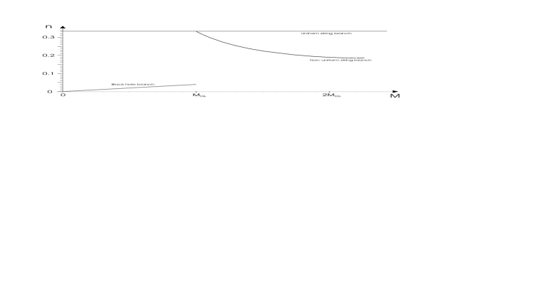
Figure 1: $(M,n)$ phase diagram for $d=5$ containing the black hole branch, the uniform string branch and the non-uniform string branch of Wiseman.

A comment is in order here. In Figure 1 we have continued the linear behavior of $n$ as function of $M$ all the way up to $M=M_{\rm GL}$. To see why we expect (7.1) to be approximately valid up to $M=\,M_{\rm GL}$, we consider the function $F(\rho,\theta)$ in (3.11). We have included the first correction in $F(\rho,\theta)$ but not the second one. The value of $\rho$ for which the second correction is of equal size as the first correction is given by $\rho^{2}=8\pi^{2}\zeta(d-2)/((d-1)(d-2)\zeta(d))$. For $d=5$ this gives that not including the second term in $F(\rho,\theta)$ is a good approximation for $\rho\ll 2.8$. In terms of the horizon radius this means that $\rho_{0}\ll 2.8$. Thus, we see that (7.1) should be valid for $\rho_{0}^{3}\ll 21$ which translates to $\mu\ll 9$ and furthermore to $M\ll 4\,M_{\rm GL}$. This therefore makes it likely that (7.1) is valid to a good approximation up to $M\simeq M_{\rm GL}$.

8 Discussion and conclusions

The main results of this paper are:

• We have found the complete metric for small black holes on cylinders $\mathbb{R}^{d-1}\times S^{1}$. For $\tilde{\rho}\gg\rho_{0}$ the metric is given by (4.9) while for $\rho_{0}\leq\tilde{\rho}\ll 1$ the metric is given by (5.3)-(5.4). The metric is valid to first order in $\rho_{0}^{d-2}$, which means to first order in the mass.

• We have found the corrected thermodynamics using the metric (5.3)-(5.4). The corrected thermodynamics is (6.3)-(6.5). We can summarize the corrected thermodynamics in the formula (6.10)

  $$\frac{\delta\log S}{\delta\log\mu}=\frac{d-1}{d-2}\left(1+\frac{\zeta(d-2)}{2(d-1)\Omega_{d-1}}\,\mu+\mathcal{O}(\mu^{2})\right)\ ,$$

  where $\mu$ is the rescaled mass in (6.8).

• We obtained in (6.9) the corrected relative binding energy $n$ which we found to increase when increasing the mass. If we allow variations of the circumference $L$ of the cylinder, the first law of thermodynamics is $\delta M=T\delta S+nML^{-1}\delta L$ [22, 23]. Therefore, a non-zero $n$ means that the black hole does not behave point-like (a point-like object would have $\delta M=0$ under a variation of $L$). Qualitatively, this means that the physics of black holes on cylinders are governed by the shape of the event horizon rather than that of the singularity.

The fact that we were able to find the complete metric describing small black holes can be taken as a confirmation on a basic assumption about the nature of black holes: That black holes obey the principle of locality.

The “principle of locality for black holes” means here that we believe that sufficiently small black holes should not be influenced by the global structure of the space-time. Thus, for any locally flat space-time it should be so that small black holes behave like in flat space. For a black hole on the cylinder $\mathbb{R}^{d-1}\times S^{1}$ this means that as the mass $M\rightarrow 0$ it become more and more like a $(d+1)$-dimensional Schwarzschild black hole. Using for example (6.7) this assumption on black holes on cylinders is seen to be equivalent to the assumption that $n\rightarrow 0$ for $M\rightarrow 0$. That we in this paper are able to find a metric for small black holes is thus a non-trivial consistency check on this assumption.

A connected assumption is the one of Section 2.3 that as the black hole become smaller it behaves more and more like a point-like object. This assumption leads to the prediction (2.22) of the Fourier modes for the complete black hole branch, as seen in Section 2.3. The argument of Section 2.3 used that $n\rightarrow 0$ for $M\rightarrow 0$ and that Newtonian physics should take over most of the space-time as $M\rightarrow 0$. Again, that we found the complete metric for small black holes is a non-trivial check on these arguments. It seems therefore reasonable to expect that the complete black hole branch have the Fourier modes given by (2.22).

We have also seen that the ansatz (2.10) proposed in [15] and proven in [18, 22] is highly succesful in describing small black holes. This paper can therefore be seen as a confirmation on the usefulness of this ansatz.

The success of the methods of this paper makes it natural to ask whether they can be continued and one can find higher order corrections to black holes on cylinders. We believe that indeed is the case.

Obviously, finding more corrections would be highly interesting in view of the ongoing discussion on which scenario of the black hole/black string transitions that is the correct one. That is unfortunately still unclear, even after the numerical work on black holes on the cylinder $\mathbb{R}^{4}\times S^{1}$ in [24, 25].

Finally, we comment that the non-zero relative binding energy that we found for small black holes on cylinders means that the so-called “Uniqueness Hypothesis” of [21, 22], stating that there only exists one neutral and static black object for a given $M$ and $n$, still seem to hold for black holes and strings on cylinders. If the relative binding energy would have been zero the Uniqueness Hypothesis would be violated due to the black hole copies (see [22] and Section 6).

Appendix A Thermodynamics in the $(R,v)$ and $(\tilde{\rho},\tilde{\theta})$ coordinates

Thermodynamics in the $(R,v)$ coordinates

We review here the thermodynamics in terms of the $(R,v)$ coordinates defined by the ansatz (2.10), as found in [15]. Define

$$A_{h}\equiv A(R,v)|_{R=R_{0}}\ ,$$ (A.1)

which, as shown in [15], is independent of $v$. Let furthermore the asymptotic behavior of $K(R,v)$ for $R\rightarrow\infty$ be written as

$$K(R,v)=1-\chi\frac{R_{0}^{d-3}}{R^{d-3}}+\mathcal{O}(R^{-2(d-3)})\ ,$$ (A.2)

then we have using (2.8)-(2.9) with (2.5)-(2.7) [15, 21]

$$M=\frac{\Omega_{d-2}}{8G_{\rm N}}R_{0}^{d-3}\frac{(d-1)(d-3)}{d-2-n}\ ,\ \ n=\frac{1-(d-2)(d-3)\chi}{d-2-(d-3)\chi}\ ,$$ (A.3)

$$T=\frac{d-3}{4\pi\sqrt{A_{h}}R_{0}}\ ,\ \ S=\frac{2\pi\Omega_{d-2}}{4G_{\rm N}}\sqrt{A_{h}}R_{0}^{d-2}\ .$$ (A.4)

(A.3)-(A.4) gives the thermodynamics of solutions described in the ansatz (2.10).

It was derived in [22, 23] that the first law of thermodynamics

$$\delta M=T\delta S\ ,$$ (A.5)

holds for the black hole solutions. Obviously on the black hole branch we can consider all the quantities as being functions of $R_{0}$ only. Therefore, we can express (A.5) as $\delta M/\delta R_{0}=T\delta S/\delta R_{0}$. Thus, in terms of the above defined quantities $A_{h}$ and $n$ the first law is equivalent to

$$\frac{1}{2}\frac{R_{0}}{A_{h}}\frac{\delta A_{h}}{\delta R_{0}}=\frac{d-1}{(d-2-n)^{2}}R_{0}\frac{\delta n}{\delta R_{0}}-\frac{1-(d-2)n}{d-2-n}\ .$$ (A.6)

Thermodynamics in the $(\tilde{\rho},\tilde{\theta})$ coordinates

We review here the thermodynamics thermodynamics in terms of the $(\tilde{\rho},\tilde{\theta})$ coordinates defined by (3.6). Define

$$\tilde{A}_{h}\equiv\tilde{A}(\tilde{\rho},\tilde{\theta})|_{\tilde{\rho}=\rho_{0}}\ .$$ (A.7)

The thermodynamics is then

$$M=\frac{\Omega_{d-1}}{16\pi G_{\rm N}}\rho_{0}^{d-2}\frac{(d-1)(d-2)}{d-2-n}\ ,\ \ T=\frac{d-2}{4\pi\rho_{0}\sqrt{\tilde{A}_{h}}}\ ,\ \ S=\frac{\Omega_{d-1}}{4G_{\rm N}}\rho_{0}^{d-1}\sqrt{\tilde{A}_{h}}\ .$$ (A.8)

We note that for $\tilde{A}_{h}=1$ and $n=0$ this thermodynamics is that of a Schwarzschild black hole in $d+1$ dimensions.

The first law in the form (A.6) gives

$$\frac{1}{2}\rho_{0}(\log\tilde{A}_{h})^{\prime}=\frac{(d-1)n}{d-2-n}+\frac{d-1}{(d-2-n)^{2}}\rho_{0}n^{\prime}\ ,$$ (A.9)

where the prime denotes the derivative with respect to $\rho_{0}$. This relation is of importance in the text.

Appendix B Derivation of general spherical metric

We start with a $d+1$ dimensional metric of the form

$$ds^{2}=-fdt^{2}+f^{-1}e^{q}d\tilde{\rho}^{2}+e^{q-(d-2)u}\tilde{\rho}^{2}d\tilde{\theta}^{2}+e^{u}\tilde{\rho}^{2}\sin^{2}\tilde{\theta}d\Omega_{d-2}^{2}\ ,\ \ f=1-\frac{\rho_{0}^{d-2}}{\tilde{\rho}^{d-2}}\ ,$$ (B.1)

with $q=q(\tilde{\rho})$ and $u=u(\tilde{\rho})$, i.e. without any $\tilde{\theta}$ dependence. We see that (B.1) is in the form of the ansatz (3.6) with $\tilde{A}=e^{q}$ and $\tilde{K}=e^{u}$. We want to analyze the solutions of the vacuum Einstein equations with the metric (B.1).

From $R_{\tilde{\rho}\tilde{\theta}}=0$ we immediately get that $q^{\prime}=(d-1)u^{\prime}$. We can therefore write $q=s+(d-1)u$ where $s$ is a constant. Write now $d\Omega_{d-2}^{2}=d\phi_{1}^{2}+\sin^{2}\phi_{1}d\phi_{2}^{2}+\cdots+\sin^{2}\phi_{1}\cdots\sin^{2}\phi_{d-3}d\phi_{d-2}^{2}$, where $\phi_{1},...,\phi_{d-2}$ are the angles of $S^{d-2}$. If we consider the Einstein equation $R^{\phi_{1}}_{\ \phi_{1}}=0$ it is easy to see that that equation only can be satisfied provided $s=0$. Therefore, the metric (B.1) reduces to

$$ds^{2}=-fdt^{2}+f^{-1}e^{(d-1)u}d\tilde{\rho}^{2}+e^{u}\tilde{\rho}^{2}\left(d\tilde{\theta}^{2}+\sin^{2}\tilde{\theta}d\Omega_{d-2}^{2}\right)\ ,\ \ f=1-\frac{\rho_{0}^{d-2}}{\tilde{\rho}^{d-2}}\ .$$ (B.2)

We now consider the solutions of the vacuum Einstein equations for this metric, still with $u=u(\tilde{\rho})$. The remaining non-trivial Einstein equations gives the two equations

$$u^{\prime\prime}-\frac{d-3}{\tilde{\rho}}u^{\prime}-\frac{d-2}{2}(u^{\prime})^{2}=0\ ,$$ (B.3)

$$\left(1-\frac{\rho_{0}^{d-2}}{\tilde{\rho}^{d-2}}\right)u^{\prime\prime}+\frac{d-1}{\tilde{\rho}}u^{\prime}-\frac{\rho_{0}^{d-2}}{\tilde{\rho}^{d-2}}\frac{1}{\tilde{\rho}}u^{\prime}-\frac{2(d-2)}{\tilde{\rho}^{2}}\left(e^{(d-2)u}-1\right)=0\ .$$ (B.4)

Defining

$$G(\tilde{\rho})=\exp\left(-\frac{d-2}{2}u(\tilde{\rho})\right)\ ,$$ (B.5)

we see that (B.3) becomes

$$G^{\prime\prime}-\frac{d-3}{\tilde{\rho}}G^{\prime}=0\ .$$ (B.6)

The most general solution to this equation is

$$G=c_{1}\rho^{d-2}+c_{2}\ ,$$ (B.7)

with $c_{1}$ and $c_{2}$ being arbitrary constants. Putting (B.7) into (B.4) we get that (B.4) is fulfilled if and only if

$$\rho_{0}^{d-2}c_{1}c_{2}+c_{2}^{2}=1\ .$$ (B.8)

Thus, we get that the most general vacuum solution with metric (B.2) is given by

$$\exp\left(-\frac{d-2}{2}u\right)=\frac{1-w^{2}}{w}\frac{\tilde{\rho}^{d-2}}{\rho_{0}^{d-2}}+w\ ,$$ (B.9)

where $w$ is an arbitrary constant. This means that the most general vacuum solution with metric (B.1) is given by $q=(d-1)u$ and (B.9).

References

- [1] R. C. Myers, “Higher dimensional black holes in compactified space- times,” Phys. Rev. D35 (1987) 455.
- [2] A. R. Bogojevic and L. Perivolaropoulos, “Black holes in a periodic universe,” Mod. Phys. Lett. A6 (1991) 369–376.
- [3] D. Korotkin and H. Nicolai, “A periodic analog of the Schwarzschild solution,” gr-qc/9403029.
- [4] A. V. Frolov and V. P. Frolov, “Black holes in a compactified spacetime,” Phys. Rev. D67 (2003) 124025, hep-th/0302085.
- [5] W. Israel and K. Khan, “Collinear particles and Bondi dipoles in General Relativity,” Nuovo Cim. 33 (1964) 331.
- [6] H. Weyl, “Zur gravitationstheorie,” Ann. Phys. 54 (1917) 117.
- [7] R. Emparan and H. S. Reall, “Generalized Weyl solutions,” Phys. Rev. D65 (2002) 084025, hep-th/0110258.
- [8] P.-J. De Smet, “Black holes on cylinders are not algebraically special,” Class. Quant. Grav. 19 (2002) 4877–4896, hep-th/0206106.
- [9] R. Gregory and R. Laflamme, “Black strings and p-branes are unstable,” Phys. Rev. Lett. 70 (1993) 2837–2840, hep-th/9301052.
- [10] R. Gregory and R. Laflamme, “The instability of charged black strings and p-branes,” Nucl. Phys. B428 (1994) 399–434, hep-th/9404071.
- [11] G. T. Horowitz and K. Maeda, “Fate of the black string instability,” Phys. Rev. Lett. 87 (2001) 131301, hep-th/0105111.
- [12] R. Gregory and R. Laflamme, “Hypercylindrical black holes,” Phys. Rev. D37 (1988) 305.
- [13] S. S. Gubser, “On non-uniform black branes,” Class. Quant. Grav. 19 (2002) 4825–4844, hep-th/0110193.
- [14] T. Wiseman, “Static axisymmetric vacuum solutions and non-uniform black strings,” Class. Quant. Grav. 20 (2003) 1137–1176, hep-th/0209051.
- [15] T. Harmark and N. A. Obers, “Black holes on cylinders,” JHEP 05 (2002) 032, hep-th/0204047.
- [16] G. T. Horowitz, “Playing with black strings,” hep-th/0205069.
- [17] B. Kol, “Topology change in general relativity and the black-hole black-string transition,” hep-th/0206220.
- [18] T. Wiseman, “From black strings to black holes,” Class. Quant. Grav. 20 (2003) 1177–1186, hep-th/0211028.
- [19] T. Harmark and N. A. Obers, “Black holes and black strings on cylinders,” Fortsch. Phys. 51 (2003) 793–798, hep-th/0301020.
- [20] B. Kol and T. Wiseman, “Evidence that highly non-uniform black strings have a conical waist,” Class. Quant. Grav. 20 (2003) 3493–3504, hep-th/0304070.
- [21] T. Harmark and N. A. Obers, “New phase diagram for black holes and strings on cylinders,” hep-th/0309116.
- [22] T. Harmark and N. A. Obers, “Phase structure of black holes and strings on cylinders,” hep-th/0309230.
- [23] B. Kol, E. Sorkin, and T. Piran, “Caged black holes: Black holes in compactified spacetimes I – theory,” hep-th/0309190.
- [24] E. Sorkin, B. Kol, and T. Piran, “Caged black holes: Black holes in compactified spacetimes. II: 5d numerical implementation,” hep-th/0310096.
- [25] H. Kudoh and T. Wiseman, “Properties of Kaluza-Klein black holes,” hep-th/0310104.
- [26] R. Casadio and B. Harms, “Black hole evaporation and large extra dimensions,” Phys. Lett. B487 (2000) 209–214, hep-th/0004004.
- [27] R. Casadio and B. Harms, “Black hole evaporation and compact extra dimensions,” Phys. Rev. D64 (2001) 024016, hep-th/0101154.
- [28] G. T. Horowitz and K. Maeda, “Inhomogeneous near-extremal black branes,” Phys. Rev. D65 (2002) 104028, hep-th/0201241.
- [29] B. Kol, “Speculative generalization of black hole uniqueness to higher dimensions,” hep-th/0208056.
- [30] E. Sorkin and T. Piran, “Initial data for black holes and black strings in 5d,” Phys. Rev. Lett. 90 (2003) 171301, hep-th/0211210.
- [31] M. W. Choptuik et al., “Towards the final fate of an unstable black string,” Phys. Rev. D68 (2003) 044001, gr-qc/0304085.
- [32] R. Emparan and R. C. Myers, “Instability of ultra-spinning black holes,” JHEP 09 (2003) 025, hep-th/0308056.
- [33] J. Traschen and D. Fox, “Tension perturbations of black brane spacetimes,” gr-qc/0103106.
- [34] P. K. Townsend and M. Zamaklar, “The first law of black brane mechanics,” Class. Quant. Grav. 18 (2001) 5269–5286, hep-th/0107228.
- [35] T. Harmark and N. A. Obers, “Work in progress,”.
- [36] J. Traschen, “A positivity theorem for gravitational tension in brane spacetimes,” hep-th/0308173.
- [37] T. Shiromizu, D. Ida, and S. Tomizawa, “Kinematical bound in asymptotically translationally invariant spacetimes,” gr-qc/0309061.