IPPP/03/60 DCPT/03/120 $N$-point Amplitudes in Intersecting Brane Models

Abstract

We derive general and complete expressions for $N$-point tree-level amplitudes in Type II string models with matter fields localised at D-brane intersections.

1 Introduction

Since their discovery, and their subsequent relation to gauge theories, D-branes have become established as a central element in the development of phenomenologically viable string models. They facilitate immediate and straightforward construction of models with interesting gauge groups. However, the requirement of chirality in any physically realistic model leads to a restricted number of possible D-brane set-ups. An important class are the intersecting brane models [1, 2]. This scenario exploits the fact that chiral fermions can arise at the intersection of two branes at angles [3], hence the spectrum of fermions is determined by the intersection numbers of the D-branes which wrap some compact space. As a consequence, a simple and rather attractive topological explanation of family replication is obtained.

The intersecting brane scenario has been remarkably successful in producing semi-realistic models, for example, Refs. [1, 4, 5, 6, 7, 8, 9, 10, 11, 12, 13, 14, 15, 16]. Models similar to the Standard Model can be obtained [17, 18, 19, 20, 21, 22, 23] and furthermore viable constructions with $N=1$ supersymmetry have been developed [24, 25, 26, 27, 28, 29, 30, 31], although this latter possibility is more difficult to achieve. A more detailed analysis of the phenomenology of such models is currently in progress, for example [32, 33, 34, 35]. In particular, computations of Yukawa couplings [36, 37] and flavour changing neutral currents [38] have been performed.

In this paper we generalise the methods used for the computation of the three and four point amplitudes in [39, 40] to the case of $N$-point amplitudes, In particular, deriving complete expressions for both the classical and quantum contributions.

Our analysis will be based on the technology discussed in [41, 42, 43] for closed strings on orbifolds. This is due to an analogy between twisted closed string states on orbifolds and open strings at brane intersections. This analogy has been discussed previously in ref. [40] and will be briefly recapped in our first section. We then proceed to a determination of the classical part of the general $4$-point amplitude. This calculation is then generalised to the N-point case along with a prescription for obtaining the wrapped contributions to the amplitude in the case of toroidal geometry. Next, we use conformal field theory techniques to evaluate the quantum contribution to a general four point amplitude with three independent angles. This calculation is then fully generalised in the determination of the quantum contribution to the $N$-point tree level amplitude. As a consistency check, we proceed to demonstrate that the $(N-1)$-point amplitude can be obtained as a limiting case of the $N$-point amplitude.

Finally, as an example of the application of our results, we analyse the situation of four independent sets of branes. In particular, we discuss the relevant process $q_{L}q_{R}\rightarrow e_{L}e_{R}$ which, depending on the D-brane geometry, is a purely stringy effect, or has a field theory limit corresponding to a Higgs exchange. In the latter case, we extract the Higgs pole and determine the mass of the Higgs purely from the four point amplitude. Throughout this work we will focus on the case of D6-branes wrapping the compact internal space $T^{2}\times T^{2}\times T^{2}$, however, our results are easily adapted to other cases.

2 Closed and open string twisted states

Let us begin by briefly reviewing the analogy between closed strings on oribfolds and open strings at D-brane intersections. This analogy allows us to employ the CFT techniques developed in [42, 41], which forms a basis for our analysis.

An open string stretched between two D-branes intersecting at an angle $\pi\vartheta$, as depicted in figure 1, has the boundary conditions,

$$\begin{array}[]{l}\partial_{\tau}X^{2}(0)=\partial_{\sigma}X^{1}(0)=0,\\ \partial_{\tau}X^{1}(\pi)+\partial_{\tau}X^{2}(\pi)\cot(\pi\vartheta)=0,\\ \partial_{\sigma}X^{2}(\pi)-\partial_{\sigma}X^{1}(\pi)\cot(\pi\vartheta)=0.\end{array}$$ (1)

Thus we can determine the holomorphic solutions to the string equation of motion to be,

$$\begin{array}[]{l}\partial X(z)=\sum_{k}\alpha_{k-\vartheta}z^{-k+\vartheta-1},\\ \partial\bar{X}(z)=\sum_{k}\bar{\alpha}_{k+\vartheta}z^{-k-\vartheta-1},\end{array}$$ (2)

where $z=-e^{\tau-i\sigma}$ is the worldsheet coordinate and has domain the upper-half complex plane. This domain is extended to the entire complex plane using the ‘doubling trick’, i.e. we define,

$$\partial X(z)=\left\{\begin{array}[]{ll}\partial X(z)&\mbox{Im}(z)\geq 0\\ \bar{\partial}\bar{X}(\bar{z})&\mbox{Im}(z)<0\end{array}\right.,$$ (3)

and similarly for $\partial\bar{X}(z)$.

Figure 1: A ‘twisted’ open string state

Now the mode expansion of a closed string state in the presence of a $\mathbb{Z}_{N}$ orbifold twist field, is identical to (2) with the replacement $\vartheta=\frac{1}{N}$. Hence, we see that there is a natural correspondence between open strings stretched between intersecting branes and a twisted closed string state on an orbifold. To take account of this correspondence, we must introduce a twist field $\sigma_{\vartheta}(w,\bar{w})$ for the open string, this field changes the boundary conditions of $X$ to be those of eq.(1), where the intersection point of the two D-branes is at $X(w,\bar{w})$. Proceeding as in the closed string case we obtain the OPEs,

$$\begin{array}[]{l}\partial X(z)\sigma_{\vartheta}(w,\bar{w})\sim(z-w)^{-(1-\vartheta)}\tau_{\vartheta}(w,\bar{w}),\\ \partial\bar{X}(z)\sigma_{\vartheta}(w,\bar{w})\sim(z-w)^{-\vartheta}\tau^{\prime}_{\vartheta}(w,\bar{w}),\end{array}$$ (4)

where $\tau^{\prime}_{\vartheta}$ and $\tau_{\vartheta}$ are excited twist fields. The local monodromy conditions for transportation around $\sigma_{\vartheta}(w,\bar{w})$ are simply determined from the OPEs to be,

$$\begin{array}[]{l}\partial X(e^{2\pi i}(z-w))=e^{2\pi i\vartheta}\partial X(z-w),\\ \partial\bar{X}(e^{2\pi i}(z-w))=e^{-2\pi i\vartheta}\partial\bar{X}(z-w).\end{array}$$ (5)

The mode expansion for $X$ is then,

$$X(z,\bar{z})=\sqrt{\frac{\alpha^{\prime}}{2}}\sum_{k}\left(\frac{\alpha_{k-\vartheta}}{k-\vartheta}z^{-k+\vartheta}+\frac{\tilde{\alpha}_{k+\vartheta}}{k+\vartheta}\bar{z}^{-k-\vartheta}\right),$$ (6)

with the right and left moving modes being mapped into upper and lower half planes. A similar mode expansion is obtained for the fermions with the obvious addition of $\frac{1}{2}$ to the boundary conditions for NS sectors.

The correspondence with twisted states on orbifolds (or conifolds) can be seen geometrically as in figure 2. This figure shows two identical three point diagrams which are sewn together at their edges. An open string living at the intersection is doubled up to form a twisted closed string. As a result we expect to recover the famous $\mbox{open string}\sim\sqrt{\mbox{closed string}}$ relation. However, we also note that the intersection angles in this case are more general than the rather restrictive ones found in supersymmetric orbifolds of closed strings.

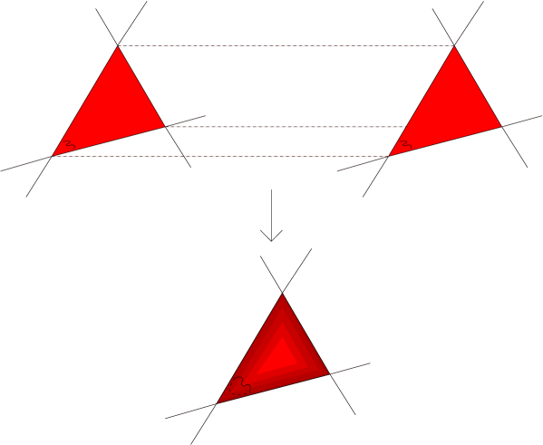
Figure 2: Identifying open strings to form closed strings

3 The classical part of the $N$-point function

We now proceed to an analysis of the $N$-point function for string states localised at $N$ distinct D-brane intersections. We assume the $N$ D-branes form the boundary of an $N$-sided polygon, with vertices $f_{i}$ and interior angles $\pi\vartheta_{i}$ such that,

$$\sum_{i=1}^{N}\vartheta_{i}=N-2.$$ (7)

The D-brane intersecting $f_{i}$ and $f_{i+1}$ is labelled the $i^{th}$ D-brane. We will consider two distinct cases for our compactification space M,

• planar, $M=\mathbb{R}^{2}\times\mathbb{R}^{2}\times\mathbb{R}^{2}$,

• and toroidal, $M=T_{2}\times T_{2}\times T_{2}$.

The planar case is useful for illustrating the methods used in the computation without adding extra complication, and furthermore, will turn out to give the leading order contribution in the more realistic toroidal scenario. Due to our choice of $M$, the amplitude can be factorised into a product of three identical contributions, one from each of the three subfactors (i.e. $\mathbb{R}^{2}$ or $T_{2}$). In the following, we will therefore concentrate on the contribution from one such subfactor.

We denote the spacetime coordinates for a particular subfactor by $X=X^{1}+iX^{2}$ and $\bar{X}=X^{1}-iX^{2}$. The bosonic field $X$ can be split up into a classical piece, $X_{cl}$, and a quantum fluctuation, $X_{qu}$. The amplitude then factorises into classical and quantum components,

$$Z=\sum_{\langle X_{cl}\rangle}e^{-S_{cl}}Z_{qu},$$ (8)

where,

$$S_{cl}=\frac{1}{4\pi\alpha}\left(\int d^{2}z(\partial X_{cl}\bar{\partial}\bar{X}_{cl}+\bar{\partial}X_{cl}\partial\bar{X}_{cl})\right).$$ (9)

$X_{cl}$ must satisfy the string equation of motion and possess the correct asymptotic behaviour near the polygon vertices.

3.1 Determining the classical $4$-point function for the plane

Before discussing the calculation of the classical contribution to the general $N$-point amplitude, let us first consider the simpler four point case. The $4$-point function requires $4$ twist operators, $\sigma_{\vartheta_{i}}(z_{i},\bar{z}_{i})$, one for each polygon vertex or D-brane intersection. These twist operators are attached to the boundary of the tree-level disc diagram which can be conformally mapped to the upper-half plane. Hence, using $SL(2,\mathbb{R})$ invariance we set $z_{1}=0$, $z_{2}=x_{2}$, $z_{3}=1$ and $z_{4}=x_{\infty}$. The classical solution, $\partial X_{cl}$, is determined up to a normalisation constant by its holomorphicity and asymptotic behaviour at each D-brane intersection, which is given by the OPEs (4). Thus,

$$\begin{array}[]{ll}\partial X_{cl}(z)=a\omega(z),&\partial\bar{X}_{cl}(z)=\bar{a}\omega^{\prime}(z),\\ \bar{\partial}X_{cl}(\bar{z})=b\bar{\omega}^{\prime}(\bar{z}),&\bar{\partial}\bar{X}_{cl}(\bar{z})=\bar{b}\bar{\omega}(\bar{z}),\end{array}$$ (10)

where,

$$\begin{array}[]{ll}\omega(z)=\prod_{i=1}^{4}(z-x_{i})^{-(1-\vartheta_{i})}&\omega^{\prime}(z)=\prod_{i=1}^{4}(z-x_{i})^{-\vartheta_{i}},\end{array}$$ (11)

and $a,\bar{a},b,\bar{b}\in\mathbb{C}$ are normalisation constants. Using the doubling trick to define $\partial X_{cl}$ on the entire complex plane, we require $a^{*}=\bar{b}$ and $\bar{a}=b^{*}$ (upto a phase).

The normalisation of the classical solutions are determined from the global monodromy conditions, i.e. the transformation of $X$ as it is transported around more than one twist operator, such that the net twist is zero. We determine this from the action of a single twist operator, $\sigma_{\vartheta}(w,\bar{w})$, which in the planar case acts to transform $X(z,\bar{z})$ as,

$$X(e^{2\pi i}z,e^{-2\pi i}\overline{z})=e^{2\pi i\vartheta}X+(1-e^{2\pi i\vartheta})f,$$ (12)

where f is the intersection point of the two D-branes. This can be seen from the local monodromy conditions (5) and the fact that $f$ must be left invariant. The global monodromy of $X$ is then simply a product of such actions. Note, if we split $X$ up into a classical and quantum part, then the classical field should have exactly the same behaviour as the full field. Hence, the boundary conditions for $X_{qu}$ ignores the shift $(1-e^{2\pi i\vartheta})f$ leaving,

$$X_{qu}(e^{2\pi i}z,e^{-2\pi i}\overline{z})=e^{2\pi i\vartheta}X_{qu}.$$ (13)

For the $4$-point case, there exists $2$ independent contours, $C_{i}$, $i=1,2$, with net twist zero. Each $C_{i}$ is a Pochammer loop, which is illustrated in figure 3. The $2$ independent global monodromy conditions for the classical field are,

$$\Delta_{C_{i}}X_{cl}=e^{-\pi i(\vartheta_{i}-\vartheta_{i+1})}4\sin(\pi\vartheta_{i})\sin(\pi\vartheta_{i+1})(f_{i+1}-f_{i})=\oint_{C_{i}}dz\partial X_{cl}(z)+\oint_{C_{i}}d\overline{z}\bar{\partial}X_{cl}(\bar{z}).$$ (14)

Figure 3: The Pochammer loop $C_{i}$ with net twist zero, branch cuts lie along the dashed lines.

The contour integrals required can be written as,

$$\begin{array}[]{l}\oint_{C_{i}}dz\omega(z)=e^{-\pi i(\vartheta_{i}-\vartheta_{i+1})}4\sin(\pi\vartheta_{i})\sin(\pi\vartheta_{i+1})F_{i},\\ \oint_{C_{i}}d\bar{z}\bar{\omega}^{\prime}(\bar{z})=e^{-\pi i(\vartheta_{i}-\vartheta_{i+1})}4\sin(\pi\vartheta_{i})\sin(\pi\vartheta_{i+1})\bar{F}^{\prime}_{i},\end{array}$$ (15)

where,

$$\begin{array}[]{ll}F_{i}=\int_{x_{i}}^{x_{i+1}}\prod_{j=1}^{4}(y-x_{j})^{-(1-\vartheta_{j})}dy&F^{\prime}_{i}=\int_{x_{i}}^{x_{i+1}}\prod_{j=1}^{4}(y-x_{j})^{-\vartheta_{j}}dy.\end{array}$$ (16)

Hence (14) can be simplified to,

$$\begin{array}[]{ll}aF_{i}+b\bar{F}^{\prime}_{i}=f_{i+1}-f_{i}&i=1,2.\end{array}$$ (17)

Using these conditions we can determine a and b. Construct the classical solutions $\partial X_{cl,1}$ and $\partial X_{cl,2}$, with coefficients $\alpha_{i},\beta_{i}$ as in (10) and which have the simple global monodromy,

$$\begin{array}[]{ll}\alpha_{i}F_{j}+\beta_{i}\bar{F}^{\prime}_{j}=\delta_{ij},&i,j=1,2.\end{array}$$ (18)

Then,

$$\begin{array}[]{ll}\alpha_{1}=\frac{\bar{F}^{\prime}_{2}}{F_{1}\bar{F}^{\prime}_{2}-F_{2}\bar{F}^{\prime}_{1}},&\alpha_{2}=-\frac{\bar{F}^{\prime}_{1}}{F_{1}\bar{F}^{\prime}_{2}-F_{2}\bar{F}^{\prime}_{1}},\\ \beta_{1}=-\frac{F_{2}}{F_{1}\bar{F}^{\prime}_{2}-F_{2}\bar{F}^{\prime}_{1}},&\beta_{2}=\frac{F_{1}}{F_{1}\bar{F}^{\prime}_{2}-F_{2}\bar{F}^{\prime}_{1}}.\end{array}$$ (19)

It follows, that to satisfy (17) for $i=1,2$, we require,

$$\begin{array}[]{l}a=(f_{2}-f_{1})\alpha_{1}+(f_{3}-f_{2})\alpha_{2},\\ b=(f_{2}-f_{1})\beta_{1}+(f_{3}-f_{2})\beta_{2}.\end{array}$$ (20)

Finally, using (9) and (10) the classical contribution to the $4$-point function in the planar case is given by,

$$S_{cl}(x_{2})=\frac{1}{4\pi\alpha^{\prime}}\left(|a|^{2}I(x_{2})+|b|^{2}I^{\prime}(x_{2})\right),$$ (21)

where,

$$\begin{array}[]{ll}I(x_{2})=\int d^{2}z|\omega(z)|^{2}&I^{\prime}(x_{2})=\int d^{2}z|\omega^{\prime}(z)|^{2}.\end{array}$$ (22)

We now proceed to the generalisation of this calculation to the $N$-point case.

3.2 Generalisation to the $N$-point function

The $N$-point function requires $N$ twist operators, $\sigma_{\vartheta_{i}}(x_{i})$, where $x_{1}=0$, $x_{N-1}=1$ and $x_{N}=\infty$. The classical solution is again determined up to a normalisation constant by it’s holomorphicity and asymptotic behaviour at each D-brane intersection. However, in this case we may generalise our expressions for the classical solutions to,

$$\begin{array}[]{ll}\partial X_{cl}(z)=a\omega(z),&\partial\bar{X}_{cl}(z)=\rho(z)\omega^{\prime}(z),\\ \bar{\partial}X_{cl}(\bar{z})=\bar{\rho}(\bar{z})\bar{\omega}^{\prime}(\bar{z}),&\bar{\partial}\bar{X}_{cl}(\bar{z})=a^{*}\bar{\omega}(\bar{z}),\end{array}$$ (23)

where $\rho(z)$ is a polynomial of degree $p$ and,

$$\begin{array}[]{ll}\omega(z)=\prod_{i=1}^{N}(z-x_{i})^{-(1-\vartheta_{i})}&\omega^{\prime}(z)=\prod_{i=1}^{N}(z-x_{i})^{-\vartheta_{i}}.\end{array}$$ (24)

This modification obviously does not change the asymptotics of $X_{cl}$ at the D-brane intersections. However, if we consider the contribution to $S_{cl}$,

$$\int d^{2}z\bar{\partial}X_{cl}\partial\bar{X}_{cl}=\int d^{2}z|\rho(z)|^{2}|\omega^{\prime}(z)|^{2},$$ (25)

we see that this converges only if $p\leq N-4$. Notice that for $N=4$ the expressions in (23) reduce to those of our previous case in (10). We can define a useful basis for $\rho(z)$ given by,

$$\rho^{i}(z)=\prod_{\stackrel{{\scriptstyle\mbox{\scriptsize$j=2$}}}{{\mbox{\scriptsize$(j\neq i$)}}}}^{N-2}(z-x_{j}), \hskip 14.22636pti=2,..,N-2.$$ (26)

Our generalised classical solutions can then be expressed in the form,

$$\begin{array}[]{ll}\bar{\partial}X_{cl}(\bar{z})=b_{i}^{*}\bar{\Omega}^{\prime i}(\bar{z}),&\partial\bar{X}_{cl}(z)=b_{i}\Omega^{\prime i}(z),\end{array}$$ (27)

where,

$$\Omega^{\prime i}=\omega^{\prime}(z)\rho^{i}(z).$$ (28)

In the $N$-point case our classical solutions require $N-2$ normalisation constants. However, we now have $N-2$ Pochammer loops, $C_{l}$, $i=l,..,N-2$ to which we can apply the global monodromy condition (14). The required contour integrals are given by the $(N-2)\times(N-2)$ matrix $W^{i}_{l}$, defined by

$$\begin{array}[]{l}W^{1}_{l}=\oint_{C_{l}}dz\omega(z)=e^{-i\pi(\vartheta_{l}-\vartheta_{l+1})}4\sin(\pi\vartheta_{l})\sin(\pi\vartheta_{l+1})F_{l}^{1},\\ W^{i}_{l}=\oint_{C_{l}}d\bar{z}\bar{\Omega}^{\prime i}(\bar{z})=e^{-i\pi(\vartheta_{l}-\vartheta_{l+1})}4\sin(\pi\vartheta_{l})\sin(\pi\vartheta_{l+1})F_{l}^{i},\end{array}$$ (29)

where,

$$\begin{array}[]{ll}F_{l}^{1}=\int_{x_{l}}^{x_{l+1}}\omega(y)dy,&\\ F_{l}^{i}=\int_{x_{l}}^{x_{l+1}}\bar{\omega}^{\prime}(y)\rho^{i}(y)dy,&i=2,..,N-2.\end{array}$$ (30)

Substituting into (14) we obtain the global monodromy conditions,

$$\begin{array}[]{ll}c_{i}F^{i}_{l}=f_{l+1}-f_{l}&l=1,..,N-2,\end{array}$$ (31)

with $c_{i}=(a,b^{*}_{2},..,b^{*}_{N-2})$. So we now have $N-2$ conditions for $N-2$ constants. Thus,

$$c_{i}(x_{2},..,x_{N-2})=\sum_{l=1}^{N-2}(f_{l+1}-f_{l})(F^{-1})_{i}^{l}.$$ (32)

Finally, we determine the classical contribution to the $N$-point function in the planar case to be,

$$S_{cl}(x_{2},..,x_{N-2})=\frac{1}{4\pi\alpha^{\prime}}\left(|a|^{2}I+\sum_{i,j}b_{i}^{*}b_{j}I^{\prime}_{\bar{i}j}\right),$$ (33)

where,

$$\begin{array}[]{ll}I(x_{2},..,x_{N-2})=\int d^{2}z|\omega(x)|^{2},&I^{\prime}_{\bar{i}j}(x_{2},..,x_{N-2})=\int d^{2}z\bar{\Omega}^{\prime i}(\bar{z})\Omega^{\prime j}(z).\end{array}$$ (34)

Note that, for $N=4$ this reduces to (21).

3.3 Determining the classical $N$-point function for the torus

We next consider the more phenomenologically interesting case of $M=T^{2}\times T^{2}\times T^{2}$ and show that our previous result is simply the leading order contribution. Define, $T^{2}=\mathbb{R}^{2}/\Lambda$, where $\Lambda$ is a lattice with basis vectors $v_{x}=R_{x}(1,0)$ and $v_{y}=R_{y}(0,1)$. We denote by $(n,m)$ a non-trivial cycle winding $n$ times around the cycle defined by $v_{x}$ and $m$ times around the cycle defined by $v_{y}$. The $i^{th}$ D-brane then wraps the cycle $(n_{i},m_{i})$ and the number of intersections with the $j^{th}$ D-brane is given by the intersection number,

$$I_{ij}=n_{i}m_{j}-n_{j}m_{i}.$$ (35)

These cycles gives rise to an infinite number of polygons which wrap the torus and contribute to the N-point function. Our computation will follow the same general methodology described above, but with some important modifications.

On introduction of toroidal geometry, the action of our twist operators must be generalised to not only rotate $X_{cl}$ but also to shift by a lattice translation. Hence (12) is modified to

$$X(e^{2\pi i}z,e^{-2\pi i}\overline{z})=e^{2\pi i\vartheta}X+(1-e^{2\pi i\vartheta})(f+v),$$ (36)

where $v\in\Lambda^{*}$, a coset of $\Lambda$. It follows, that on integrating around $C_{i}$, the portion of integration around each vertex takes $X_{cl}(z,\bar{z})$ from one D-brane to another, while integrating between the two vertices introduces a shift along the $i^{th}$ D-brane. Define $\vec{L}_{i,i+1}$ to lie in the direction $f_{i+1}-f_{i}$, with magnitude the distance along the $i^{th}$ D-brane between successive copies of the $(i+1)^{th}$ D-brane. Then the shift must be of the form $f_{i+1}-f_{i}+v_{i}$ where $v_{i}=q_{i}|I_{i,i+1}|\vec{L}_{i,i+1}\in\Lambda^{*}$, $q_{i}\in\mathbb{Z}$, as illustrated in figure 4. Such lattice shifts give rise to polygons wrapping the torus, and hence to further contributions to the $N$-point function. Note that, if the $i^{th}$ D-brane has D-branes which run parallel to it, we must modify our shift vector to $v_{i}=q_{i}gcd(\{|I_{k,i+1}||k\in P(i)\})\vec{L}_{i,i+1}$, where $P(i)$ is the set of all D-branes parallel to the $i^{th}$ D-brane and $gcd$ stands for the greatest common divisor.

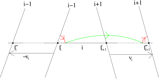
Figure 4: Transporting $X_{cl}$ around two twist fields

The global monodromy conditions are now generalised to,

$$\Delta_{C_{i}}X_{cl}=e^{-\pi i(\vartheta_{i}-\vartheta_{i+1})}4\sin(\pi\vartheta_{i})\sin(\pi\vartheta_{i+1})(f_{i+1}-f_{i}+v_{i})=\oint_{C_{i}}dz\partial X_{cl}(z)+\oint_{C_{i}}d\overline{z}\bar{\partial}X_{cl}(\bar{z}).$$ (37)

Using the contour integrals (29) we obtain,

$$\begin{array}[]{ll}c_{i}F^{i}_{l}=f_{l+1}-f_{l}+v_{l},&l=1,..,N-2.\end{array}$$ (38)

Hence, we now have,

$$c_{i}(x_{2},..,x_{N-2},q_{1},..,q_{N-2})=\sum_{l=1}^{N-2}(f_{l+1}-f_{l}+v(l))(F^{-1})_{i}^{l}.$$ (39)

Our normalisation constants are now dependent on the $q_{l}$ as well as the $x_{i}$. The $q_{l}$ define the wrapped polygons, and take values determined by the intersection numbers of the D-branes.

To determine the wrapped polygons which contribute to the $N$-point amplitude, consider extending (w.l.o.g) from vertex $f_{2}$ as depicted in figure 5. Closure of the polygon requires,

$$\sum_{i=1}^{N}v_{i}=0.$$ (40)

Assuming there are no D-branes parallel to one another and substituting,

$$|I_{i,i+1}|\vec{L}_{i,i+1}=-(n_{i}v_{x}+m_{i}v_{y}),$$ (41)

into (40) we obtain the linear diophantine equations,

$$\left(\begin{array}[]{l}q_{N}I_{N,N-1}\\ q_{N-1}I_{N,N-1}\end{array}\right)=\left(\begin{array}[]{lll}I_{N-1,1}&\ldots&I_{N-1,N-2}\\ I_{1,N}&\ldots&I_{N-2,N}\end{array}\right)\left(\begin{array}[]{l}q_{1}\\ \vdots\\ q_{N-2}\end{array}\right).$$ (42)

We can now determine our wrapped polygons by extending from $f_{2}$, taking all values of $q_{i}$, $i=1,..,N-2$ that allow for integer solutions to (42). Each such solution defines a wrapped polygon contributing to the N-point function. For example, consider the $N=3$ case. Then (42) reduces to,

$$\begin{array}[]{ll}q_{1}I_{21}=q_{3}I_{32},&q_{2}I_{21}=q_{3}I_{13}.\end{array}$$ (43)

The $q_{1}$ and $q_{2}$ which allow for integer solutions are then of the form,

$$\begin{array}[]{ll}q_{1}=\frac{l|I_{32}|}{gcd(|I_{21}|,|I_{32}|,|I_{13}|)},&q_{2}=\frac{l|I_{13}|}{gcd(|I_{21}|,|I_{32}|,|I_{13}|)},\end{array}$$ (44)

where $l\in\mathbb{Z}$. This reproduces the result found in [40, 39] for the wrapping contributions to Yukawa interactions.

Figure 5: Determining the wrapped polygons

Unfortunately, it is not possible to solve (42) in the general case, only for concrete examples. This is due to the fact that diophantine equations are usually solved algorithmically, however, it is possible to make some general remarks. We require the following result from linear algebra [44, 45],
THEOREM. Let $A\in M_{m,n}(\mathbb{Z})$. There exists $L\in SL_{m}(\mathbb{Z})$ and $R\in SL_{n}(\mathbb{Z})$ such that,

$$LAR=D=diag(d_{1},d_{2},..,d_{s},0,..,0),$$ (45)

where $d_{i}>0$, $i=1,..,s$ and $d_{i}|d_{i+1}$, $i=1,..,s-1$.
Denoting our diophantine matrix equation as $b=Ax$, we can therefore write our solution as $x=Ry$ where $y$ is a solution to the diagonal system of equations, $Dy=e$, with $e=Lb$. Since A is of size $2\times(N-2)$, we have in general two distinct cases for the form of D, corresponding to $s=1$ and $s=2$ above. However, our assumption of a convex polygon means that we only need to consider the case $s=2$. This can be deduced from the fact that the dimension of the row space of A is the same as that of D. Hence, we have the general solution,

$$\left(\begin{array}[]{l}q_{1}\\ \vdots\\ q_{N-2}\end{array}\right)=R\left(\begin{array}[]{l}e_{1}/d_{1}\\ e_{2}/d_{2}\\ l_{1}\\ \vdots\\ l_{N-4}\end{array}\right),$$ (46)

where $l_{i}$ are free integer parameters and $e_{1}$ and $e_{2}$ are functions of $q_{N}$ and $q_{N-1}$. Unfortunately, it is not possible to determine $L$ and $R$ for a general matrix $A$.

We can now write the classical contribution to the N-point function in the toroidal case as,

$$Z_{cl}(x_{2},..,x_{N-2})=\sum_{q_{1},.,q_{N-2}}e^{-Scl(x_{2},..,x_{N-2},q_{1},..,q_{N-2})},$$ (47)

where,

$$S_{cl}(x_{2},..,x_{N-2},q_{1},..,q_{N-2})=\frac{1}{4\pi\alpha^{\prime}}\left(|a|^{2}I(x_{2},..,x_{N-2})+\sum_{i,j}b_{i}^{*}b_{j}I^{\prime}_{\bar{i}j}(x_{2},..,x_{N-2})\right).$$ (48)

Note that we sum over $N-2$ variables corresponding to the $N-2$ independent sides of an $N$-sided polygon and only include $q_{i}$ such that (42) has a solution. This sum incorporates all possible wrapped polygon contributions to our classical amplitude.

3.4 Expressing $S_{cl}$ in terms of $F_{D}$

It is possible to express $S_{cl}$ solely in terms of generalised (type D Lauricella) hypergeometric functions. This allows us to express $N$-point amplitudes in a more computationally friendly manner. Firstly, since $S_{cl}$ is independent of $x_{\infty}$, we can drop the $(y-x_{\infty})$ factors from $I,I^{\prime}_{\bar{i}j}$, and $F^{i}_{l}$ i.e. they factor out from the integrals and cancel. Next consider,

$$I(x_{2},..,x_{N-2})=\int\prod_{j=2}^{N-2}|z-x_{j}|^{-2(1-\vartheta_{i})}|z|^{-2(1-\vartheta_{1})}|z-1|^{-2(1-\vartheta_{N-1})}d^{2}z.$$ (49)

Using the method of [46] to relate open and closed string amplitudes, we can split up the above integral into a product of holomorphic and antiholomorphic contour integrals. Thus,

$$I(x_{2},..,x_{N-2})=\sum_{p=2}^{N-1}(-1)^{p}\alpha_{2,p}|F^{1}_{p}||F^{1}_{1}|+\sum_{j=2}^{N-2}\sum_{p=0}^{j-1}(-1)^{j-(p+1)}\alpha_{p+1,j}|F^{1}_{j}||F^{1}_{p}|,$$ (50)

where $\alpha_{ij}=\sin(\pi\sum_{l=i}^{j}\vartheta_{l})$ and,

$$F^{1}_{N-1} =\int_{1}^{\infty}\prod_{j=1}^{N-1}(y-x_{j})^{-(1-\vartheta_{j})}\quad F^{1}_{0} =\int_{-\infty}^{0}\prod_{j=1}^{N-1}(y-x_{j})^{-(1-\vartheta_{j})}.$$ (51)

We can now relate each $F^{1}_{i}$ to a type D Lauricella hypergeometric function. In particular, it can be easily seen that,

$$F^{1}_{i} =e^{i\pi\vartheta_{i}}(x_{i}-x_{i+1})^{-1+\vartheta_{i}+\vartheta_{i+1}}\prod_{\stackrel{{\scriptstyle j=1}}{{(j\neq i,i+1)}}}^{N-1}(x_{i}-x_{j})^{-(1-\vartheta_{j})}B(\vartheta_{i},\vartheta_{i+1})$$

$$\times F_{D}^{(N-3)}(\vartheta_{i},1-\vartheta_{1},..,1-\vartheta_{i-1},1-\vartheta_{i+2},..,1-\vartheta_{N-1};\vartheta_{i}+\vartheta_{i+1};\tilde{x}_{i,1},..,\tilde{x}_{i,i-1},\tilde{x}_{i,i+2},..,\tilde{x}_{i,N-1}),$$

$$F^{1}_{0} =e^{-i\pi(\vartheta_{N}+1)}B(\vartheta_{N},\vartheta_{1})\times$$

$$\times F_{D}^{(N-3)}(\vartheta_{N},1-\vartheta_{2},..,1-\vartheta_{N-2};\vartheta_{1}+\vartheta_{N};1-x_{2},..,1-x_{N-2}),$$

$$F^{1}_{N-1} =B(\vartheta_{N},\vartheta_{N-1})F_{D}^{(N-3)}(\vartheta_{N},1-\vartheta_{2},..,1-\vartheta_{N-2};\vartheta_{N}+\vartheta_{N-1};x_{2},..,x_{N-2}),$$ (52)

where $\tilde{x}_{ij}=\frac{x_{i}-x_{i+1}}{x_{i}-x_{j}}$ and $B(a,b)$ is the beta function. The $I^{\prime}_{\bar{i}j}$ can also be treated as above.

These expressions provide us with a simpler handle on the classical contribution to the $N$-point amplitude. Let us first consider the simple case of $N=4$. We will then see that for general $N$ and under certain circumstances, we can minimise the classical action to the sum of the polygon areas in each of the torus subfactors.

3.5 The general four point amplitude

Consider a four point amplitude of the general type depicted in figure 6. The above expressions will enable us to express (21) and the extension to wrapped polygons more explicitly. In this case, $S_{cl}$ is simply a function of $x_{2}$ and the wrapping numbers $q_{1}$ and $q_{2}$, and our expressions for the $F^{1}_{i}$ involve simple hypergeometric functions of the form ${}_{2}F_{1}(a,b,c;x)$. From (3.4) we explicitly obtain,

Figure 6: Generic 4 point diagram

$$\begin{array}[]{l}F^{1}_{0}=e^{-i\pi(1+\vartheta_{4})}B(\vartheta_{4},\vartheta_{1}){}_{2}F_{1}(\vartheta_{4},1-\vartheta_{2},\vartheta_{1}+\vartheta_{4};1-x_{2}),\\ F^{1}_{1}=e^{-i\pi(\vartheta_{2}+\vartheta_{3})}x_{2}^{-1+\vartheta_{1}+\vartheta_{2}}B(\vartheta_{1},\vartheta_{2}){}_{2}F_{1}(\vartheta_{1},1-\vartheta_{3},\vartheta_{1}+\vartheta_{2};x_{2}),\\ F^{1}_{2}=e^{-i\pi(-1+\vartheta_{3})}(1-x_{2})^{-1+\vartheta_{2}+\vartheta_{3}}B(\vartheta_{2},\vartheta_{3}){}_{2}F_{1}(\vartheta_{3},1-\vartheta_{1},\vartheta_{2}+\vartheta_{3};1-x_{2}),\\ F^{1}_{3}=B(\vartheta_{4},\vartheta_{3}){}_{2}F_{1}(\vartheta_{4},1-\vartheta_{2},\vartheta_{4}+\vartheta_{3};x_{2}).\end{array}$$ (53)

Note that $F^{1}_{i}=F_{i}$ and $F^{2}_{i}=\bar{F}^{\prime}_{i}$ as defined in subsection 3.1. We can relate $F^{1}_{0}$ and $F^{1}_{3}$ to $F_{1}$ and $F_{2}$ as follows,

$$\begin{array}[]{l}|F^{1}_{0}|=\frac{\sin(\pi\vartheta_{2})}{\sin(\pi\vartheta_{1})(1-\alpha\beta)}\left(|F_{2}|+\beta|F_{1}|\right),\\ |F^{1}_{3}|=\frac{\sin(\pi\vartheta_{2})}{\sin(\pi\vartheta_{3})(1-\alpha\beta)}\left(|F_{1}|+\alpha|F_{2}|\right),\end{array}$$ (54)

where,

$$\begin{array}[]{ll}\alpha=-\frac{\sin(\pi(\vartheta_{1}+\vartheta_{2}))}{\sin(\pi\vartheta_{1})},&\beta=-\frac{\sin(\pi(\vartheta_{2}+\vartheta_{3}))}{\sin(\pi\vartheta_{3})}.\end{array}$$ (55)

Substituting into (50) we obtain,

$$I(x_{2})=\frac{\sin(\pi\vartheta_{2})}{1-\alpha\beta}(\beta|F_{1}|^{2}+2|F_{1}||F_{2}|+\alpha|F_{2}|^{2}).$$ (56)

Furthermore, for this simple case, we can derive the relations,

$$\begin{array}[]{l}|F^{\prime}_{1}|=(1-x_{2})^{1-\vartheta_{2}-\vartheta_{3}}x_{2}^{1-\vartheta_{1}-\vartheta_{2}}\gamma(|F_{1}|+\alpha|F_{2}|),\\ |F^{\prime}_{2}|=(1-x_{2})^{1-\vartheta_{2}-\vartheta_{3}}x_{2}^{1-\vartheta_{1}-\vartheta_{2}}\gamma(|F_{2}|+\beta|F_{1}|),\end{array}$$ (57)

where,

$$\gamma=\frac{\Gamma(1-\vartheta_{2})\Gamma(1-\vartheta_{4})}{\Gamma(\vartheta_{1})\Gamma(\vartheta_{3})}.$$ (58)

Note that $I^{\prime}$ and $F^{\prime}_{i}$ are obtained from $I$ and $F_{i}$ by the substitution $\vartheta_{i}\rightarrow 1-\vartheta_{i}$. Hence, $I^{\prime}(x_{2})$ can now also be obtained in terms of $|F_{1}|$ and $|F_{2}|$ simply by letting $\vartheta_{i}\rightarrow 1-\vartheta_{i}$ in (56) and substituting in (57). We also require the expressions,

$$\begin{array}[]{ll}|a|=\left(\frac{v_{21}|F^{\prime}_{2}|+v_{32}|F^{\prime}_{1}|}{|F_{1}||F^{\prime}_{2}|+|F_{2}||F^{\prime}_{1}|}\right),&|b|=\left(\frac{v_{32}|F_{1}|-v_{21}|F_{2}|}{|F_{1}||F^{\prime}_{2}|+|F_{2}||F^{\prime}_{1}|}\right),\end{array}$$ (59)

where $v_{21}=|f_{2}-f_{1}+v_{1}|$ and $v_{32}=|f_{3}-f_{2}+v_{2}|$. This allows us to obtain the following contribution to the classical action from a single $T_{2}$,

$$S^{T_{2}}_{cl}(\tau,v_{21},v_{32})=\frac{\sin(\pi\vartheta_{2})}{4\pi\alpha^{\prime}}\left(\frac{((v_{21}\tau-v_{32})^{2}+\gamma\gamma^{\prime}(v_{21}(\beta+\tau)+v_{32}(1+\alpha\tau))^{2})}{(\beta+2\tau+\alpha\tau^{2})}\right),$$ (60)

where $\tau(x_{2})=\left|\frac{F_{2}}{F_{1}}\right|$ and $\gamma^{\prime}$ is obtained from $\gamma$ by the substitution $\vartheta_{i}\rightarrow 1-\vartheta_{i}$.

The complete expression for the action is just a sum of these contributions, one from each torus subfactor, i.e.

$$S_{cl}=\sum_{i=1}^{3}S^{T^{i}_{2}}_{cl}(\tau^{i},v^{i}_{21},v^{i}_{32}).$$ (61)

Now, if there is only non-zero worldsheet area in one subtorus, or if the angles (and hence $\tau^{i}$) and ratios of lengths are the same in every subtorus (i.e. the polygons are identical up to a scaling), we may use a saddle point approximation to minimise the complete $S_{cl}$. The minimum of $S^{T_{2}}_{cl}$ is given by,

$$\tau_{min}=\frac{v_{32}}{v_{21}},$$ (62)

and after some manipulation we find,

$$S^{T_{2}}_{cl}(\tau_{min})=\frac{1}{2\pi\alpha^{\prime}}\left(\frac{\sin\pi\vartheta_{1}\sin\pi\vartheta_{4}}{\sin(\pi\vartheta_{1}+\pi\vartheta_{4})}\frac{v_{14}^{2}}{2}-\frac{\sin\pi\vartheta_{2}\sin\pi\vartheta_{3}}{\sin(\pi\vartheta_{2}+\pi\vartheta_{3})}\frac{v_{23}^{2}}{2}\right).$$ (63)

We recognize this as the area/$2\pi\alpha^{\prime}$ of the four-sided polygon. Note also that at this minimum $b=0$. Hence, in this case, we see that $S_{cl}$ is minimised to the sum of the areas of the quadrilaterals from each $T^{2}$ subfactor.

As we have seen, at the minimum of $S^{T_{2}}_{cl}$ for $N=4$, $b=0$ and we obtain the area of the polygon involved in the interaction. An analogous situation also occurs in the three point case, where again $b=0$ and the action is the area of a triangle. Furthermore, it seems intuitively obvious that for general $N$, the area of the worldsheet (i.e. $S_{cl}$) has as its minimum value the area of the polygon associated with the amplitude, provided only one $S^{T^{i}_{2}}_{cl}$ is non-zero. That this is indeed the case, and this occurs when the $b_{i}=0$, can be motivated as follows.

We can express $X_{cl}$ as,

$$X_{cl}(z,\bar{z})=A+a\int^{z}\prod_{i=1}^{N}((\zeta-x_{i})^{-(1-\vartheta_{i})}d\zeta+b^{*}_{l}\int^{\bar{z}}\prod_{i=1}^{N}\overline{(\bar{\zeta}-x_{i})^{-\vartheta_{i}}}\rho^{l}(\bar{\zeta})d\bar{\zeta},$$ (64)

with $X_{cl}(x_{i})=f_{i}$ and $A\in\mathbb{C}$. The lower integration limits are left unspecified as they affect only the value of A. Differentiating gives $\partial X_{cl}$ and $\bar{\partial}X_{cl}$, as in section 3.2. Note that we expect $X_{cl}$ to be, at least locally, one to one and hence if $f_{j}=f_{i}$ we must have $x_{j}=x_{i}$. Using (64) and $X_{cl}(x_{i})=f_{i}$ allows us immediately to obtain the relation,

$$\begin{array}[]{ll}c_{l}F^{l}_{i}=f_{i+1}-f_{i}&i=1,..,N-2,\end{array}$$ (65)

which are simply the global monodromy conditions (31).

Now inserting $b_{i}=0$ in (64), we obtain a Schwarz-Christoffel map. This is the general form of a map from the upper-half complex plane to an $N$-sided polygon. Hence, integrating this over the complex plane as in (48) just gives back the area of the polygon as the classical action. In summary, we have motivated the simple rule,

The minimum of the classical action equals the sum of the polygon areas projected in each $T^{2}$ when the non-zero polygons are the same up to an overall scaling.

From now on, in keeping with the literature on Schwarz-Christoffel mappings, we will refer to the $x_{i}$ as prevertices.

3.6 Wrapping contributions

To completely determine the classical contribution to the $4$-point amplitude, we must also include contributions from polygons which wrap the tori. We need to determine what values of $q_{1}$ and $q_{2}$ to sum over to include all the wrapping contributions to the amplitude. The integers $q_{i}$ we require are simply those which allow for an integer solution to the following system of two diophantine equations obtained from (42),

$$\left(\begin{array}[]{l}q_{1}I_{21}\\ q_{2}I_{21}\end{array}\right)=\left(\begin{array}[]{ll}I_{32}&I_{42}\\ I_{13}&I_{14}\end{array}\right)\left(\begin{array}[]{l}q_{3}\\ q_{4}\end{array}\right).$$ (66)

For any fixed $q_{1}$ and $q_{2}$ this solution is unique, since the determinant of the above matrix is non-zero. However, for the general case it is not possible to solve this for our wrapped polygons, since as mentioned earlier a solution can only be generated algorithmically. However, for the simplest $b=0$ cases, we see that the the classical part of any polygon contribution to an $N$-point amplitude is essentially $e^{-\frac{1}{2\pi\alpha^{\prime}}A}$, where $A$ is the area of the wrapped polygon in the relevant $T^{2}$ torus. Hence, the leading contribution to the $N$-point function comes from the smallest polygon. This is the single unwrapped polygon from the planar case corresponding to the trivial solution to (42), i.e. all $q_{i}=0$.

In the situation where we have D-branes which are parallel, our diophantine equations (42) no longer apply. The necessary modifications can be easily determined by substituting the generalised expression,

$$v_{i}=q_{i}gcd(\{|I_{k,i+1}||k\in P(i)\})\vec{L}_{i,i+1},$$ (67)

into $\sum v_{j}=0$. To illustrate this we consider the following two cases.

3.6.1 One independent angle

Firstly, we consider the simple case of one independent angle as depicted in figure 7.

Figure 7: Two sets of parallel D-branes.

Here we have two sets of parallel branes, the $1^{st}$ and $3^{rd}$, and the $2^{nd}$ and $4^{th}$. As before, closure of the polygon results in the expression,

$$\sum_{i=1}^{4}v_{i}=0.$$ (68)

However, we now have,

$$v_{i}=q_{i}gcd(|I_{i,i+1}|,|I_{i+2,i+1}|)\vec{L}_{i,i+1},$$ (69)

for $i=1,..,4$. If we define $\vec{L}_{i,i-1}$ to lie in the direction $f_{i}-f_{i+1}$, with magnitude the distance along the $i^{th}$ brane between successive $(i-1)^{th}$ branes, we obtain the the relation,

$$-|I_{i,i-1}|\vec{L}_{i,i-1}=|I_{i,i+1}|\vec{L}_{i,i+1}=-(n_{i}v_{x}+m_{i}v_{y}).$$ (70)

Substituting (69) and (70) into (68), we obtain the intuitively obvious result $q_{1}=q_{3}$ and $q_{2}=q_{4}$. Hence, when summing over wrapping contributions we have a double sum as determined previously in [40, 39].

3.6.2 Two independent angles

Next, we consider the case of two independent angles as shown in figure 8.

Figure 8: One set of parallel D-branes.

This time we have the $1^{st}$ and $3^{rd}$ branes parallel. Hence $v_{1}$ and $v_{3}$ are still given by (69), however now $v_{2}$ and $v_{3}$ are given by the ‘non-parallel’ expression, $v_{i}=q_{i}|I_{i,i+1}|\vec{L}_{i,i+1}$. Again, substituting into (68) and simplifying using (70) we obtain,

$$\begin{array}[]{ll}q_{1}A-q_{3}A=q_{4}I_{42},&q_{2}I_{12}=q_{4}I_{41},\end{array}$$ (71)

where we have defined $gcd(|I_{12}|,|I_{23}|)=a_{1}|I_{12}|+b_{1}|I_{23}|$ and $A=a_{1}I_{21}+b_{1}I_{32}$. The second expression requires,

$$\begin{array}[]{ll}q_{2}=\frac{lI_{41}}{gcd(I_{12},I_{41})},&q_{4}=\frac{lI_{12}}{gcd(I_{12},I_{41})},\end{array}$$ (72)

where $l\in\mathbb{Z}$. Defining,

$$c(l):=\frac{lI_{12}I_{42}}{gcd(I_{12},I_{41})},$$ (73)

we obtain an infinite set of diophantine equations,

$$(q_{1}-q_{3})A=c(l),$$ (74)

labelled by $l$. For a fixed l, a solution to (74) exits if and only if $A$ divides $c(l)$. In which case, we have an infinite number of solutions given by,

$$\begin{array}[]{ll}q_{1}=\frac{klI_{12}I_{42}}{Agcd(I_{12},I_{41})},&q_{3}=\frac{(-1+k)lI_{12}I_{42}}{Agcd(I_{12},I_{41})},\end{array}$$ (75)

where $k\in\mathbb{Z}$. Hence, our wrapped polygons are determined by extending from $f_{2}$ using,

$$\begin{array}[]{ll}q_{1}=\frac{klI_{12}I_{42}}{Agcd(I_{12},I_{41})},&q_{2}=\frac{lI_{41}}{gcd(I_{12},I_{41})},\end{array}$$ (76)

and summing over $l,k\in\mathbb{Z}$ such that $q_{1}\in\mathbb{Z}$.

4 The quantum contribution

4.1 General 4-point quantum contribution

We now turn to the quantum contribution to the amplitude, beginning in this subsection with the generalization of the four fermion scattering amplitude to cases where four independent branes intersect at arbitrary angles. We wish to calculate the instanton contribution shown in figure 6.

This amplitude is given by a disc diagram with four fermionic vertex operators in the $-1/2$ picture, $V^{(a)}$ on the boundary. The diagram can then be mapped to the upper half plane with vertices on the real axis by using the same Schwarz-Christoffel mapping as discusses earlier for the classical contribution. The positions of the vertices ($x_{1}\ldots x_{4}$) will eventually be fixed by $SL(2,R)$ invariance to $0,x,1,\infty$ (where $x$ is real), so that the 4 point ordered amplitude can be written

$$\begin{array}[]{ll}S_{4}(1,2,3,4)&=(2\pi)^{4}\delta^{4}(\sum_{a}k_{a})\,A(1,2,3,4)\\ &=\frac{-i}{g_{s}l_{s}^{4}}\int_{0}^{1}dx\langle V^{(1)}(0,k_{1})V^{(2)}(x,k_{2})V^{(3)}(1,k_{3})V^{(4)}(\infty,k_{4})\rangle.\end{array}$$ (77)

To get the total amplitude we sum over all possible orderings;

$$A_{total}(1,2,3,4) = A(1,2,3,4)+A(1,3,2,4)+A(1,2,4,3)$$ (78)

$$+ A(4,3,2,1)+A(4,2,3,1)+A(4,3,1,2).$$

The vertex operators for the fermions are of the form

$$V_{i}^{(a)}(x_{a},k_{a})=const\,\,\lambda^{a}u_{\alpha}^{(i)}S_{i}^{\alpha}\sigma_{\vartheta_{i}}e^{-\phi/2}e^{ik_{a}.X}(x_{a}).$$ (79)

Here $u_{\alpha}$ is the space time spinor polarization, and $S^{\alpha}$ is the so called spin-twist operator of the form

$$S_{i}^{\alpha}=\prod_{l=1}^{5}:\exp(iq_{i}^{l}H_{l}):$$ (80)

where for D6 branes intersecting at angles we have $q_{i}^{l}=\left(\pm\frac{1}{2},\pm\frac{1}{2},\vartheta_{i}^{1}-\frac{1}{2},\vartheta_{i}^{2}-\frac{1}{2},\vartheta_{i}^{3}-\frac{1}{2}\right)$, with the relative sign of the first two entries being determined by the helicity, and $\vartheta_{i}^{m=1,2,3}$ being the angles of the $i^{\prime}$th intersection in the $m^{\prime}$th complex plane. In what follows we will frequently drop the $m$ index when we consider what is happening in a single sub-torus. For future reference we can also identify the available scalar fields at intersection $i$ coming from the NS sector; their masses are

$$\alpha^{\prime}M_{h}^{2} = \frac{1}{2}(\vartheta_{i}^{1}+\vartheta_{i}^{2}-\vartheta_{i}^{3})$$ (81)

$$\frac{1}{2}(\vartheta_{i}^{1}-\vartheta_{i}^{2}+\vartheta_{i}^{3})$$

$$\frac{1}{2}(-\vartheta_{i}^{1}+\vartheta_{i}^{2}+\vartheta_{i}^{3})$$

$$1-\frac{1}{2}(\vartheta_{i}^{1}+\vartheta_{i}^{2}+\vartheta_{i}^{3}).$$

The spin fields have conformal dimension

$$h_{i}=\frac{q_{i}^{2}}{2}.$$ (82)

Here $\sigma_{\vartheta_{i}}$ is the $\vartheta$ twist operator for the $i^{\prime}$th vertex, with conformal dimension

$$h_{i}=\frac{1}{2}\vartheta_{i}.(1-\vartheta_{i}).$$ (83)

The evaluation of the expectation value of products of vertex operators is straightforward apart from the factor involving the bosonic twist operators. This calculation can be done analogously to the closed string case [42]. In contrast to the restricted case discussed in ref.[40] with only one or two independent angles, we need to significantly modify the techniques however. In particular in the general case (with three independent angles) the contours required are the same Pochammer contours discussed for the classical monodromy conditions.

We now outline the derivation. Consider the contribution from a single complex dimension in which the branes intersect with angles $\vartheta_{i}\pi$ where $\sum\vartheta_{i}=2$ if there are no intersections. (Other topologies are possible. For example if there is a single intersection in the middle of the world-sheet we require $\sum_{i=left}\vartheta_{i}=\sum_{i=right}\vartheta_{i}$ where “left” and “right” indicate the vertices on opposing sides of the intersection.) We begin with the asymptotic behaviour of the Green function in the vicinity of the twist operators. Taking account of the world-sheet boundary by adding an image charge, the Green function can then be written

$$G(z,w;z_{i})=g(z,w;z_{i})+g(z,\overline{w};z_{i})$$ (84)

where $g(z,w;z_{i})$ is the usual Green function for the closed string. It has the following asymptotics

$$g(z,w;x_{i}) \sim \frac{1}{(z-w)^{2}}+finite\hskip 19.91684ptz\rightarrow w$$

$$\sim \frac{1}{(z-x_{i})^{-\vartheta_{i}}}\hskip 45.52458ptz\rightarrow x_{i}$$

$$\sim \frac{1}{(w-x_{i})^{-(1-\vartheta_{i})}}\hskip 28.45274ptw\rightarrow x_{i}$$

and as we have seen the holomorphic fields are proportional to

$$\partial X(z) \equiv \omega(z)=\prod_{i}(z-x_{i})^{-(1-\vartheta_{i})}$$

$$\partial\overline{X}(z) \equiv \omega^{\prime}(z)=\prod_{i}(z-x_{i})^{-\vartheta_{i}}.$$ (86)

so that this half of the Green function may now be written generically upto an additional term usually denoted $A$;

$$g(z,w;z_{i}) = \left.\omega(z)\omega^{\prime}(w)\left\{\sum_{ij}a_{ij}\frac{(z-x_{i})(z-x_{j})}{(w-x_{i})(w-x_{j})}\frac{\prod_{k}(w-x_{k})}{(z-w)^{2}}+A\right\}\right.$$

where $a_{i<j}$ and $A$ are constants. This is the most general function with the desired conformal properties that can be written down as prescribed in ref.[47]. Expanding in the various limits, we find by inspection that it has the required asymptotics if the constants satisfy

$$\sum_{i<j}a_{ij}=1$$

$$\sum_{j=i+1}^{4}a_{ij}+\sum_{j=1}^{i-1}a_{ji}=1-\vartheta_{i}$$ . (88)

Note that summing the second of these conditions over $i$ and using the $\sum_{i}(1-\vartheta_{i})=2$ condition automatically gives the first condition. Of course in the end any arbitrariness in the choice of $a_{ij}$ and $A$ must disappear from the amplitude which must be dependent on the $\vartheta_{i}^{\prime}s$ only.

Continuing, we now determine the general form of $\langle\prod_{i}\sigma_{\vartheta_{i}}\rangle$ by considering

$$\frac{\langle T(z)\prod_{i}\sigma_{\vartheta_{i}}\rangle}{\text{$\langle\prod_{i}\sigma_{\vartheta_{i}}\rangle$}} = \lim_{w\rightarrow z}[g_{(}z,w)-\frac{1}{(z-w)^{2}}]$$ (89)

$$= -\frac{1}{2}\sum_{ij}\vartheta_{i}\vartheta_{j}\frac{1}{(z-x_{i})(z-x_{j})}$$

$$+\frac{1}{2}\sum_{i<j}a_{ij}\left(\frac{1}{z-x_{i}}+\frac{1}{z-x_{j}}\right)^{2}+\frac{A}{\prod_{i}(z-x_{i})}.$$

and comparing it with the OPE of $T(z)$ with the twist operator

$$T(z)\sigma_{\vartheta_{j}}(x_{i})\sim\frac{h_{j}}{(z-x_{i})^{2}}+\frac{\partial_{x_{i}}\sigma_{{}_{\vartheta_{j}}}(x_{2})}{(z-x_{i})}+\ldots$$ (90)

The leading $(z-x_{i})^{2}$ divergences yield the correct conformal dimension of the twist operators;

$$h_{i}=\frac{1}{2}\vartheta_{i}(1-\vartheta_{i}).$$

Equating coefficients of $(z-x_{i})^{-1}$ (in order to preserve generality we postpone using $SL(2,R)$ invariance to fix $(x_{1},x_{2},x_{3},x_{4})=(0,x,1,x_{\infty})$ for the moment) yields a set of differential equations for $\langle\prod_{i}\sigma_{\vartheta_{i}}\rangle$ of the form

$$\partial_{x_{k}}\ln\left[\langle\prod_{i}\sigma_{\vartheta_{i}}\rangle\right]=\partial_{x_{k}}\ln\left[\prod_{i<j}(x_{i}-x_{j})^{a_{ij}-(1-\vartheta_{i})(1-\vartheta_{j})}\right]+\frac{A}{\prod_{i\neq k}(x_{k}-x_{i})}.$$ (91)

All that remains is to determine $A$ which can be done using monodromy conditions for $\partial_{z}X\partial_{w}\overline{X}$. We proceed as for the classical calculation and consider the global monodromy conditions arising from the two independent Pochammer loops, $C_{l=1,2}$, encircling the prevertices $x_{l}$ and $x_{l+1}$. From the local monodromy conditions for $X_{qu}$ given in (13), we see that on completing these contours the quantum part should be left invariant,

$$\Delta_{C_{l}}X_{qu}=0=\oint_{C_{l}}dz\partial X_{qu}+\oint_{C_{l}}d\overline{z}\overline{\partial}X_{qu}.$$ (92)

We now use $SL(2,R)$ invariance to fix $(x_{1},x_{2},x_{3},x_{4})=(0,x,1,x_{\infty})$. Taking the $w\rightarrow\infty$ limit, dividing by $w^{\prime}(w)$ and extracting the leading $x_{\infty}$ contributions, the monodromy condition applied to the Green functions,

$$\oint_{C_{l}}dz\,g(z,w)+\oint_{C_{l}}d\overline{z}\,h(\overline{z},w)=0\,,$$ (93)

gives

$$B\oint_{C_{l}}\overline{w}^{\prime}(\overline{z})d\overline{z}+A\oint_{C_{l}}w(z)dz=x_{\infty}\oint_{C_{l}}\sum_{i}a_{i4}(z-x_{i})w(z)dz$$ (94)

for both independent contours $C_{l=1,2}$, where $B$ is a constant. Defining $G_{l}=\int F_{l}(x)dx$ and $G^{\prime}_{l}=\int F^{\prime}_{l}(x)dx$ we can solve for $A$;

$$x_{\infty}A=(1-\vartheta_{4}-a_{24})x-a_{34}-(1-\vartheta_{4})\vartheta_{2}\left[G_{1}\partial_{x}\overline{G}^{\prime}_{2}-G_{2}\partial_{x}\overline{G}^{\prime}_{1}\right]/J.$$ (95)

where

$$J=F_{1}\overline{F_{2}^{\prime}}-F_{2}\overline{F_{1}^{\prime}}.$$

An alternative solution can be found by taking the $z\rightarrow\infty$ limit of the monodromy condition and dividing by $w(z)$;

$$x_{\infty}A=(\vartheta_{4}-a_{13})x-a_{12}-(1-\vartheta_{2})\vartheta_{4}\left[G^{\prime}_{2}\partial_{x}\overline{G_{1}}-G_{1}^{\prime}\partial_{x}\overline{G_{2}}\right]/\overline{J}.$$ (96)

A different way to get the same result is to take the previous limits, but swap interior for exterior angles. Now it is well known that integrals over the different Pochammer contours with integrands involving $w(z)$ generate solutions to a particular hypergeometric differential equation. In the present case the required equation is that satisfied by the $G_{l}$ and $G_{l}^{\prime}$ which (using $\partial_{x}G_{l}=F_{l}$) can be written;

$$(1-\vartheta_{4})\vartheta_{2}G_{l} = x(1-x)\partial F_{l}-(\vartheta_{1}+\vartheta_{2}-1+(\vartheta_{4}-\vartheta_{2})x)F_{l}$$

$$(1-\vartheta_{2})\vartheta_{4}G^{\prime}_{l} = x(1-x)\partial F^{\prime}_{l}+(\vartheta_{1}+\vartheta_{2}-1+(\vartheta_{4}-\vartheta_{2})x)F^{\prime}_{l}$$ (97)

Substituting into (95) and (96) and summing yields the desired expression for $A$;

$$\frac{2A}{x_{\infty}x(1-x)}=\partial_{x}\ln|J|-\frac{a_{23}+a_{14}}{(1-x)}-\frac{a_{34}+a_{12}}{x},$$ (98)

where

$$|J|=|F_{1}\|F_{2}^{\prime}|+|F_{2}\|F_{1}^{\prime}|.$$

We shall give a closed expression for this function (in terms of hypergeometric functions) shortly.

Finally, inserting (98) into (91), and using the relations in (88) gives

$$\langle\prod_{i}\sigma_{\vartheta_{i}}\rangle=|J|^{-\frac{1}{2}}x_{\infty}^{-\vartheta_{4}(1-\vartheta_{4})}x^{\frac{1}{2}(\vartheta_{1}+\vartheta_{2}-1)-\vartheta_{1}\vartheta_{2}}(1-x)^{\frac{1}{2}(\vartheta_{2}+\vartheta_{3}-1)-\vartheta_{2}\vartheta_{3}}.$$ (99)

Note that as promised there is no arbitrariness in the choice of $a_{ij}$. The function $|J|$ may be evaluated as;

$$\begin{array}[]{l}|J|=\\ \left(\frac{x^{1-\vartheta_{1}-\vartheta_{2}}}{(1-x)^{1-\vartheta_{2}-\vartheta_{3}}}\frac{\Gamma(1-\vartheta_{1})\Gamma(\vartheta_{3})}{\Gamma(\vartheta_{3}+\vartheta_{4})\Gamma(\vartheta_{2}+\vartheta_{3})}\,\,_{2}F_{1}[1-\vartheta_{1},\vartheta_{3},\vartheta_{2}+\vartheta_{3};1-x]\,_{2}F_{1}[1-\vartheta_{1},\vartheta_{3},\vartheta_{3}+\vartheta_{4};x]\right.\\ +\,\,\,\left.\frac{(1-x)^{1-\vartheta_{2}-\vartheta_{3}}}{x^{1-\vartheta_{1}-\vartheta_{2}}}\frac{\Gamma(\vartheta_{1})\Gamma(1-\vartheta_{3})}{\Gamma(\vartheta_{1}+\vartheta_{2})\Gamma(\vartheta_{1}+\vartheta_{4})}\,\,_{2}F_{1}[\vartheta_{1},1-\vartheta_{3},\vartheta_{1}+\vartheta_{4};1-x]\,_{2}F_{1}[\vartheta_{1},1-\vartheta_{3},\vartheta_{1}+\vartheta_{2};x]\right)\end{array}$$ (100)

upto an overall factor that will be absorbed into the normalization [39], and where ${}_{2}F_{1}$ are the standard hypergeometric functions. This is for a sub-$T_{2}$ torus of the compactified space. The contributions from the three complex planes should be multiplied together with the appropriate angles $\vartheta_{i}^{m}$ for each. As a check, note that when there is only one independent angle, $\vartheta_{1}=\vartheta_{3}=\vartheta$ and $\vartheta_{2}=\vartheta_{4}=1-\vartheta$ the function reduces to that found in ref.[40]. In addition we recover the result with two independent angles derived in ref.[39] by setting $\vartheta_{1}=1-\vartheta_{2}$ and $\vartheta_{4}=1-\vartheta_{3}$. Note that the function has crossing symmetry; it is invariant under $\vartheta_{1}\leftrightarrow\vartheta_{3}$ and $x\leftrightarrow 1-x$. Finally note that the entire expression is invariant if we swap interior for exterior angles, $\vartheta_{i}\rightarrow 1-\vartheta_{i}$.

4.2 The quantum contribution to $N$-point amplitudes

The same procedure can be carried out for $N$-point functions following the techniques in ref[43] although here modified to the tree level case. The Green function should take the form

$$g(z,w;z_{i}) = \left.\omega(z)\omega^{\prime}(w)\left\{\sum_{ij}a_{ij}\frac{(z-x_{i})(z-x_{j})}{(w-x_{i})(w-x_{j})}\frac{\prod_{k}(w-x_{k})}{(z-w)^{2}}+A(w)\right\}\right.$$

where $a_{i<j}$ satisfies the same condition as above, but now $A(w)$ is a function of the form

$$A(w)=\sum_{i>j>i^{\prime}>j^{\prime}}b_{iji^{\prime}j^{\prime}}\frac{\prod_{k}(w-x_{k})}{(w-x_{i})(w-x_{j})(w-x_{i^{\prime}})(w-x_{j^{\prime}})}$$

where $b_{iji^{\prime}j^{\prime}}$ are some coefficients. (This function may look a little lobsided since it does not involve $z$, however this is merely a consequence of the fact that the conformal weights in $\gamma(z)$ already add up to 2.) We can proceed by defining a basis for $A(z)$ as we did for dX previously;

$$A(z)=\sum_{i=2}^{N-2}d_{i}\prod_{\stackrel{{\scriptstyle\mbox{\scriptsize$j=2$}}}{{\mbox{\scriptsize$(j\neq i$)}}}}^{N-2}(z-z_{j})$$ (102)

where $z_{i}$ is again the set of $N-3$ prevertices corresponding to the prevertices that are not eventually fixed by $SL(2,R)$ invariance. It is useful in what follows to define

$$g_{s}(z,w)=\omega(z)\omega^{\prime}(w)\sum_{ij}a_{ij}\frac{(z-x_{i})(z-x_{j})}{(w-x_{i})(w-x_{j})}\frac{\prod_{k}(w-x_{k})}{(z-w)^{2}}\,,$$ (103)

and $h(\overline{z},w)$ as;

$$h(\overline{z},w)=\sum_{i,j=2}^{N-2}c_{ij}\overline{\Omega}^{\prime i}(\overline{z})\Omega^{\prime j}(w)\,,$$ (104)

where $\Omega^{\prime i}(z)$ is given by (28). In order to write down a solution to the monodromy conditions we again require the $(N-2)\times(N-2)$ matrix $W^{i}_{l}$ defined in (29), where $l$ labels the $N-2$ independent Pochammer contours. (As in the classical contribution, these integrals will generate generalized hypergeometric functions which are solutions to Appell-Lauricella systems of coupled differential equations). With these definitions a solution to the global monodromy conditions with $g$ and $h$ in the prescribed form can easily be written down as follows;

$$g(z,w) = g_{s}(z,w)-\omega(z)\sum_{l}^{N-2}(W^{-1})^{l}_{1}\oint_{C_{l}}dy\,g_{s}(y,w)$$

$$h(\overline{z},w) = -\sum_{i}^{N-2}\overline{\Omega}^{\prime i}(\overline{z})\sum_{l}^{N-2}(W^{-1})^{l}_{i}\oint_{C_{l}}dy\,g_{s}(y,w).$$ (105)

We may now insert the expression for $g_{s}(z,w)$ and extract the singular holomorphic behaviour at any one of the poles, $z_{k}$, to find the holomorphic contribution;

$$\partial_{x_{k}}\ln\left[\langle\prod_{i}\sigma_{\vartheta_{i}}\rangle\right]=\partial_{x_{k}}\ln\left[\prod_{i^{\prime}<j^{\prime}}(x_{i^{\prime}}-x_{j^{\prime}})^{-(1-\vartheta_{i^{\prime}})(1-\vartheta_{j^{\prime}})}\right]$$ (106)

If we instead extract the singular antiholomorphic behaviour near any one of the poles, $\overline{z}_{k}$, (or alternatively, as in the four point case, evaluate the holomorphic behaviour for the diagram with interior and exterior angles reversed) we find

$$\partial_{x_{k}}\ln\left[\langle\prod_{i}\sigma_{\vartheta_{i}}\rangle\right]=\partial_{x_{k}}\ln\left[\prod_{j\neq k}(x_{k}-x_{j})^{1-\vartheta_{k}}\prod_{i^{\prime}<j^{\prime}}(x_{i^{\prime}}-x_{j^{\prime}})^{-\vartheta_{i^{\prime}}\vartheta_{j^{\prime}}}\right]-\sum_{l=1}^{N-2}(W^{-1})^{l}_{k}\partial_{x_{k}}W^{k}_{l}.$$ (107)

Adding the two contributions and rearranging we get the total contribution;

$$\begin{array}[]{ll}\partial_{x_{k}}\ln\left[\langle\prod_{i}\sigma_{\vartheta_{i}}\rangle\right]&=\partial_{x_{k}}\ln\left[\prod_{j\neq k}(x_{k}-x_{j})^{\frac{1-\vartheta_{k}}{2}}\prod_{i^{\prime}<j^{\prime}}(x_{i^{\prime}}-x_{j^{\prime}})^{\frac{1}{2}(\vartheta_{i^{\prime}}+\vartheta_{j^{\prime}}-1)-\vartheta_{i^{\prime}}\vartheta_{j^{\prime}}}\right]\\ &-\frac{1}{2}\sum_{l=1}^{N-2}(W^{-1})^{l}_{k}\partial_{x_{k}}W^{k}_{l}.\end{array}$$ (108)

All that remains is to evaluate the trailing term. In order to do this, following ref.[43], we note that

$$\partial_{x_{k}}\ln|W|=\sum_{l=1}^{N-2}(W^{-1})^{l}_{k}\partial_{x_{k}}W^{k}_{l}+\sum_{j\neq k}\sum_{l=1}^{N-2}(W^{-1})^{l}_{j}\partial_{x_{k}}W^{j}_{l}.$$ (109)

By comparing the singularities as $\overline{z}\rightarrow\overline{z}_{k}$ we can evaluate the second piece;

$$\sum_{j\neq k}\sum_{l=1}^{N-2}(W^{-1})^{l}_{j}\partial_{x_{k}}W^{j}_{l}=\partial_{x_{k}}\prod_{j\neq k}(x_{k}-x_{j})^{\frac{\vartheta_{k}}{2}}.$$ (110)

Finally inserting this back into eqn.108 we arrive at the desired expression for the quantum contribution;

$$\langle\prod_{i}\sigma_{\vartheta_{i}}\rangle=|W|^{-\frac{1}{2}}\prod_{i<j}^{N-3}(x_{i}-x_{j})^{\frac{1}{2}}\,\prod_{i<j}^{N}(x_{i}-x_{j})^{\frac{1}{2}(\vartheta_{i}+\vartheta_{j}-1)-\vartheta_{i}\vartheta_{j}}.$$ (111)

This is the main result of this section. One may verify that when $N=4$ it gives the earlier 4 point result; the $W_{l}^{i}$ matrix is now a $2\times 2$ matrix of the usual hypergeometric integrals in (15) whose determinant is proportional to $|J|$.

5 The complete amplitude and applications

Together with the classical contribution, this expression may now be used to find, for example, the full amplitude for 4 fermion interactions on arbitrary sets of four D-branes. For example let us recap the current-current four fermion interaction. First we collect the remaining contributions together. These are

$$ghosts\times\langle e^{-\phi/2}(0)e^{-\phi/2}(x)e^{-\phi/2}(1)e^{-\phi/2}(x_{\infty})\rangle = x_{\infty}^{\frac{1}{2}}x^{-\frac{1}{4}}(1-x)^{-\frac{1}{4}}$$

$$\langle e^{-ip_{1}.X}e^{-ip_{2}.X}e^{-ip_{3}.X}e^{-ip_{4}.X}\rangle = x^{2\alpha^{\prime}p_{1}.p_{2}}(1-x)^{2\alpha^{\prime}p_{2}.p_{3}}$$

$$\langle e^{iq_{1}.H}e^{iq_{2}.H}e^{iq_{3}.H}e^{iq_{4}.H}\rangle_{cmp} = \prod_{m}^{3}x_{\infty}^{\vartheta_{4}^{m}(1-\vartheta_{4}^{m})-\frac{1}{4}}x^{\vartheta_{1}^{m}\vartheta_{2}^{m}-\frac{1}{2}(\vartheta_{1}^{m}+\vartheta_{2}^{m})+\frac{1}{4}}\times$$ (112)

$$(1-x)^{\vartheta_{2}^{m}\vartheta_{3}^{m}-\frac{1}{2}(\vartheta_{2}^{m}+\vartheta_{3}^{m})+\frac{1}{4}}$$

where the last piece is for the three compactified tori factors only. The final piece comes from the uncompactified part of the fermions and is chirality dependent. Assume that the fermions are all of the same chirality. Then we have

$$q_{1,3} = (\pm\frac{1}{2},\pm\frac{1}{2},\ldots.)$$

$$q_{2,4} = (\pm\frac{1}{2},\mp\frac{1}{2},\ldots.)$$ (113)

Calling the first two elements $\tilde{q}_{i}$ we get an additional factor

$$\langle e^{-iq_{1}.H}e^{-iq_{2}.H}e^{-iq_{3}.H}e^{-iq_{4}.H}\rangle_{non-cmp}=x_{\infty}^{\tilde{q}_{4}.(\tilde{q}_{1}+\tilde{q}_{2}+\tilde{q}_{3})}x^{\tilde{q}_{1}.\tilde{q}_{2}}(1-x)^{\tilde{q}_{2}.\tilde{q}_{3}}=x_{\infty}^{-\frac{1}{2}}$$ (114)

where we have imposed $\sum_{i}^{4}q_{i}^{l}=0$ for all $l$ (note that $\sum_{i}^{4}\vartheta_{i}^{m}=2$ ensures that this is satisfied for the internal components), whereupon the fermions reduce to the two spinor components of left chirality fields as follows

$$\widetilde{q_{1}} = -\tilde{q}_{3}=\pm(\frac{1}{2},\frac{1}{2})$$

$$\widetilde{q_{2}} = -\tilde{q}_{4}=\pm(\frac{1}{2},-\frac{1}{2}).$$ (115)

Identifying the two $\pm$possibilities with the Weyl spinor indices $\alpha$ of the fermions $u_{\alpha}$, we see that in $u_{\alpha}^{(1)}\overline{u}_{\dot{\beta}}^{(2)}u_{\gamma}^{(3)}\overline{u}_{\dot{\delta}}^{(4)}$ we have opposite $\alpha\gamma$ and $\dot{\beta}\dot{\delta}$ indices which we may write as

$$\varepsilon_{\alpha\gamma}\varepsilon_{\dot{\beta}\dot{\delta}}=-2\sigma_{\alpha\dot{\beta}}^{\mu}\overline{\sigma}_{\mu\dot{\delta}\gamma}$$ (116)

giving the fermion factor $\overline{u}^{(1)}\gamma_{\mu}u^{(2)}\overline{u}^{(4)}\gamma^{\mu}u^{(3)}$. Adding the other factors above we find that dependence on $\vartheta_{i}^{m}$ cancels between the bosonic twist fields and the spin-twist fields giving

$$\begin{array}[]{lll}A(1,2,3,4)&=&-g_{s}\alpha^{\prime}(\lambda^{1}\lambda^{2}\lambda^{3}\lambda^{4}+\lambda^{4}\lambda^{3}\lambda^{2}\lambda^{1})\int_{0}^{1}dx\,\,x^{-1-\alpha^{\prime}s}(1-x)^{-1-\alpha^{\prime}t}\frac{1}{\prod_{m}^{3}|J^{m}|^{1/2}}\\ &&\times\left[\overline{u}^{(2)}\gamma_{\mu}u^{(1)}\overline{u}^{(4)}\gamma^{\mu}u^{(3)}\right]\sum e^{-S_{cl}(x)}\end{array}$$ (117)

where |$J^{m}|$ is the contribution from the $m^{\prime}$th internal complex dimension, we have reinstated the Chan-Paton factors, and where $s=-(k_{1}+k_{2})^{2}$, $t=-(k_{2}+k_{3})^{2}$, $u=-(k_{1}+k_{3})^{2}$ are the usual Mandlestam variables.

5.1 Obtaining the $(N-1)$-point amplitude from the $N$-point amplitude

Consistency requires that the $(N-1)$-point amplitude be obtainable from the $N$-point amplitude as a limiting case. Consider the set-up depicted in figure 9. We can reduce the $N$-point amplitude down to an $(N-1)$-point amplitude as follows. Take a single prevertex, $x_{i}$ say, and let it coalesce with $x_{i+1}$. Shifting a single prevertex of course potentially adjusts the entire polygon. However we may keep side 12, that is $f_{12}$, fixed by readjusting $a$ and keep $f_{N1}$ fixed by readjusting $b$. All $f_{j-1,j}$ can then be kept fixed by readjusting $x_{j}$ upto side $f_{i-2,i-1}$ and continuing after $f_{i+1,i+2}$. This operation (which is always possible) coalesces $f_{i}$ and $f_{i+1}$ by adjusting only the lengths of the three adjacent sides $f_{i-1,i}$, $f_{i,i+1}$, $f_{i+1,i+2}$, whilst leaving the rest of the polygon and all the angles unchanged.

The quantum contribution in (111) should reduce in the correct manner as two prevertices coalesce like this, and indeed it does. The discussion is similar to the one loop closed string diagram discussion of ref.[43], so we shall just describe the salient points. In particular when two twist fields at $x_{i}$ and $x_{j}$ come together we should recover an amplitude consistent with

$$\sigma_{\vartheta_{i}}(x_{i})\sigma_{\vartheta_{j}}(x_{j})\sim(x_{i}-x_{j})^{k_{ij}}\sigma_{\vartheta_{i}+\vartheta_{j}-1}$$ (118)

where $k_{ij}$ is to be determined by equating the conformal dimensions on each side. We find that $k_{ij}=-(1-\vartheta_{i})(1-\vartheta_{j})$ when $\vartheta_{i}+\vartheta_{j}\geq 1$ and $k_{ij}=-\vartheta_{i}\vartheta_{j}$ when $\vartheta_{i}+\vartheta_{j}\leq 1$. We have to verify that the amplitude yields the correct factors asymptotically. The basis of $N-2$ Pochammer loops evolves into $N-3$ loops as two points coalesce. When the two adjacent points come together the local behaviour of $\partial X$ is given by $\omega(z)\sim z^{-(1-\vartheta_{i})}(z-\delta)^{-(1-\vartheta_{i+1})}$ where the first prevertex we arbitrarily set to $0$ and the second to $\delta$. One can check, from our expressions (3.4) for the $F_{i}$, that the $\omega$ contour integrals around the loop “trapped” between the two vertices diverge as $(x_{i}-x_{i+1})^{\vartheta_{i}+\vartheta_{i+1}-1}$ if $\vartheta_{i}+\vartheta_{i+1}<1$ and are convergent otherwise. The opposite is true for the $\Omega^{\prime}$ integrals so that at coalescence, including the divergent factors from $|W|^{-1/2}\prod_{i<j}(x_{i}-x_{j})^{1/2}$, we have

$$\langle\prod_{j}\sigma_{\vartheta_{j}}\rangle\sim(x_{i}-x_{i+1})^{\frac{1\pm 1}{2}(\vartheta_{i}+\vartheta_{i+1}-1)-\vartheta_{i}\vartheta_{i+1}}\langle\prod_{j\neq i}\sigma_{\vartheta_{j}}\rangle$$ (119)

where we take a plus sign if $\vartheta_{i}+\vartheta_{i+1}\geq 1$ and minus if $\vartheta_{i}+\vartheta_{i+1}<1$, yielding the expected behaviour in (118).

The classical contribution to the amplitude can be dealt with in a similar fashion. We denote by $\bar{S}_{cl}$, the classical action for the $N$-point amplitude with the identification $x_{i}=x_{i+1}$, and by $\tilde{S}_{cl}$ the action we would expect for the $(N-1)$-point amplitude obtained by reduction from the $N$-point amplitude. This notation will also be employed in this subsection to distinguish other quantities between the two cases. We now show that $\bar{S}_{cl}=\tilde{S}_{cl}$.

For the $(N-1)$-point case obtained by reduction from the $N$-point case as depicted in figure 9, we have the following relations determined by the geometry of the parent amplitude,

$$\begin{array}[]{llll}f^{\prime}_{j}=f_{j}&\vartheta^{\prime}_{j}=\vartheta_{j}&x^{\prime}_{j}=x_{j}&\mbox{For $j=1,..,i-1$},\\ f^{\prime}_{j}=f_{j+1}&\vartheta^{\prime}_{j}=\vartheta_{j+1}&x^{\prime}_{j}=x_{j+1}&\mbox{For $j=i+1,..,N-1$},\end{array}$$ (120)

and also,

$$\begin{array}[]{lll}f^{\prime}_{i}=f_{i+1}=f_{i}&\vartheta^{\prime}_{i}=-1+\vartheta_{i}+\vartheta_{i+1}&x^{\prime}_{i}=x_{i+1}.\end{array}$$ (121)

Using these expressions it is simple to deduce that $\bar{I}=\tilde{I}$ and furthermore,

$$\begin{array}[]{ll}\bar{I}^{\prime}_{\bar{l}m}=\tilde{I}^{\prime}_{\overline{g(l)}g(m)},&l,m=1,..,i-1,i+1,..,N-2,\\ \bar{I}^{\prime}_{\bar{i}m}=\bar{I}^{\prime}_{\overline{i+1},m},\end{array}$$ (122)

where,

$$g(k)=\left\{\begin{array}[]{ll}k&k=1,..,i-1\\ k-1&k=i+1,..,N-2.\end{array}\right.$$ (123)

We also need to examine the global monodromy conditions in the $N$-point and $(N-1)$-point cases. For this we require the following easily obtained relations,

$$\begin{array}[]{ll}\bar{F}^{k}_{j}=\tilde{F}^{g(k)}_{g(m)},&k,j=1,..,i-1,i+1,..,N-2,\\ \bar{F}^{i}_{j}=\bar{F}^{i+1}_{j},&F^{k}_{i}=0.\end{array}$$ (124)

Then, we can see that the monodromy conditions are the same in both cases with the identification,

$$\begin{array}[]{ll}\bar{c}_{k}=\tilde{c}_{g(k)},&k=1,..,i-1,i+2,..,N-2,\\ \bar{c}_{i+1}+\bar{c}_{i}=\tilde{c}_{i}.\end{array}$$ (125)

Finally, substituting (122) and (125) into our expression for $\bar{S}_{cl}$ given in (33) we obtain $\tilde{S}_{cl}$. Hence the $N$-point amplitude reduces to that of an $(N-1)$-point amplitude as required.

Figure 9: Reducing the $N$-point amplitude to the $(N-1)$-point amplitude.

5.2 Application: Higgs exchange and flavour violation

The general 4-point amplitude is required where there are four independent branes. In models which reproduce the Standard Model (or supersymmetric variants thereof) the relevant processes are therefore $q_{L}q_{R}\rightarrow e_{L}e_{R}$ as shown in figure 10, and necessarily involve 2 left and 2 right chirality fields.

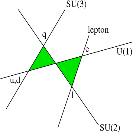
Figure 10: t-channel Higgs exchange as “double instanton”

The higgs field appears at the $SU(2)$-$U(1)$ brane intersection and so this process is the equivalent of t-channel Higgs exchange in the field theory limit. Indeed since the instanton suppression goes as $e^{-Area/2\pi\alpha^{\prime}}$ we expect to find the product of two Yukawas. The amplitude should go as

$$\frac{Y_{u}Y_{e}}{t-M_{h}^{2}}$$

or the $s$ channel equivalent, and we shall shortly verify the appearance of the Higgs pole and the correctly normalized Yukawas.

However it is also interesting to note that, merely as a result of geometry, there can be significantly larger contributions than one would expect in field theory. This is because the Higgs exchange involves the product of two Yukawa couplings. In our case this would only be the case if the lepton brane was lying to the right of the intersection (in the figure) at which the higgs is located. Then the area of the 4 point instanton is indeed the sum of the two Yukawa triangles, and the product is what appears in the amplitude. If on the other hand the lepton brane is lying to the left of the intersection, the contribution goes like $Y_{u}/Y_{e}$ and can be significantly enhanced for low string scales. In the (unrealistic) limit that the lepton brane is lying on top of the SU(3) brane in all sub-$T_{2}$tori, there is no Yukawa suppression at all in this process. Note however that there should be an overall stringy suppression as there is no field theory limit and therefore no pole. Thus one expects a contribution like

$$\frac{Y_{u}/Y_{e}}{M_{s}^{2}}$$

We shall now show how this behaviour emerges from the amplitude. To anticipate the calculation, when the situation is as in figure 10, the action is minimized in the limit $x\rightarrow 1$ corresponding to the field theory limit. In this limit we will recover the Higgs pole with the required mass from the $x$-integral. If there is no Higgs intersection then the action is minimized for finite $0<x<1$. In the simplest cases we can use a saddle point approximation as we did earlier to obtain an expression that goes as the area of the polygon with a $1/M_{s}^{2}$ suppression as expected. However generically such a simple saddle point approximation will not exist, and the $\tau^{m}$ parameters in each sub-torus will take different values. In this case interesting flavour structure can emerge.

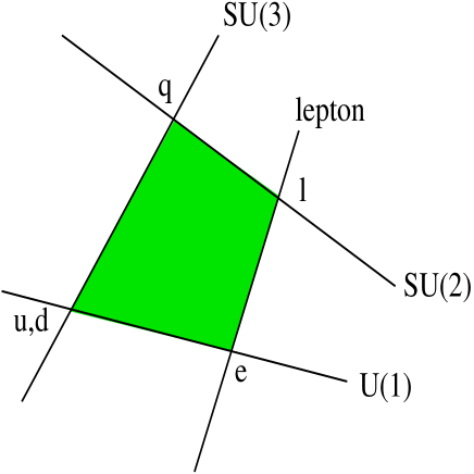
Figure 11: Equivalent instanton contribution to flavour changing

In order to show how this behaviour arises we first determine the amplitude. We are interested in the operator $(\overline{q}_{L}^{(3)}q_{R}^{(2)})(\overline{e}_{R}^{(1)}e_{L}^{(4)})$ for which the uncompactified part of the fermions now have charges

$$\widetilde{q_{1}} = -\tilde{q}_{4}=\pm(\frac{1}{2},\frac{1}{2})$$

$$\widetilde{q_{2}} = -\tilde{q}_{3}=\pm(\frac{1}{2},-\frac{1}{2}).$$ (126)

We get slightly different factors from the current-current operator. In particular

$$\langle e^{-iq_{1}.H}e^{-iq_{2}.H}e^{-iq_{3}.H}e^{-iq_{4}.H}\rangle_{non-cmp} = x_{\infty}^{\tilde{q}_{4}.(\tilde{q}_{1}+\tilde{q}_{2}+\tilde{q}_{3})}x^{\tilde{q}_{1}.\tilde{q}_{2}}(1-x)^{\tilde{q}_{2}.\tilde{q}_{3}}$$ (127)

$$= x_{\infty}^{-\frac{1}{2}}x^{\tilde{q}_{1}.\tilde{q}_{2}}(1-x)^{\tilde{q}_{2}.\tilde{q}_{3}}=x_{\infty}^{-\frac{1}{2}}(1-x)^{-\frac{1}{2}}.$$

The additional half-integer power in the $t$-channel looks unusual, but it will make sense when we extract the Higgs pole in the $x\rightarrow 1$ limit. An additional difference compared to the current-current case is that particles of one chirality take the opposite Weyl index to that of the opposing chirality. Using Weyl notation, in $\overline{u}_{\dot{\alpha}}^{(3)}\overline{u}_{\dot{\beta}}^{(2)}u_{\gamma}^{(1)}u_{\delta}^{(4)}$ we now have opposite $\dot{\alpha}\dot{\beta}$ and $\gamma\delta$ indices which (writing as $\varepsilon_{\dot{\alpha}\dot{\beta}}\varepsilon_{\gamma\delta}$) just contracts the $\overline{q}_{L}q_{R}$ and $\overline{e}_{L}e_{R}$ fermions. The final expression for the amplitude is (in four component notation) simply

$$\begin{array}[]{lll}A(1,2,3,4)&=&-g_{s}\alpha^{\prime}\,\int_{0}^{1}dx\,\,x^{-1-\alpha^{\prime}s}(1-x)^{-1-\alpha^{\prime}t}\frac{(1-x)^{-\frac{1}{2}}}{\prod_{m}^{3}|J^{m}|^{1/2}}\\ &&\,\,\,\,\times\left[(\overline{u}^{(3)}u^{(2)})(\overline{u}^{(1)}u^{(4)})\right]\sum e^{-S_{cl}(x)}\end{array}$$ (128)

The classical action is given by (61) in terms of the different $\tau$ in each sub-torus. It is easy to show that when the diagram has an intersection in a particular sub-torus, as in figure 10, the contribution to the action from that subtorus is a monotonically decreasing function of $x$. Hence the sum of the contributions is minimized by taking the limit $x\rightarrow 1$. Assuming that $1-\vartheta_{2}-\vartheta_{3}>0$, the relevant limits are

$$Lim_{x\rightarrow 1}(\tau) = -\beta$$

$$Lim_{x\rightarrow 1}(J) = (1-x)^{(-1+\vartheta_{2}+\vartheta_{3})}\,\frac{1}{\gamma}\,\,\eta(\vartheta_{2},\vartheta_{3})\eta(1-\vartheta_{1},1-\vartheta_{4})$$ (129)

where

$$\eta(\vartheta_{i},\vartheta_{j})=\left(\frac{\Gamma(\vartheta_{i})\Gamma(\vartheta_{j})\Gamma(1-\vartheta_{i}-\vartheta_{j})}{\Gamma(1-\vartheta_{i})\Gamma(1-\vartheta_{j})\Gamma(\vartheta_{i}+\vartheta_{j})}\right)^{\frac{1}{2}}$$ (130)

The normalization of the amplitudes and Yukawas can be obtained in this limit as in ref.[39]. We take the limit where the 4-point function with no intersection $\rightarrow$ the $3$-point. The normalization factor for the general $4$-point function is

$$2\pi\prod_{m=1}^{3}\sqrt{\frac{4\pi}{\gamma_{m}}\,\frac{\eta(1-\vartheta_{2}^{m},1-\vartheta_{3}^{m})}{\eta(\vartheta_{1}^{m},\vartheta_{4}^{m})}}$$ (131)

and the Yukawas take the form found in ref[39];

$$Y_{23}(A_{m})=16\pi^{\frac{5}{2}}\prod_{m}^{3}\eta(1-\vartheta_{2}^{m},1-\vartheta_{3}^{m})\,\sum_{m}e^{-A_{m}/2\pi\alpha^{\prime}}$$ (132)

where $A_{m}$ is the projected area of the triangles in the $m$’ th 2-torus. Once we add the intersection the interior $\vartheta_{1},\,\vartheta_{4}$ angles become exterior and should be replaced by $1-\vartheta_{1},\,1-\vartheta_{4}$ respectively. The constraint on the interior angles is now $\vartheta_{1}+\vartheta_{4}=\vartheta_{2}+\vartheta_{3}$ because of the intersection. Looking at $Lim_{x\rightarrow 1}(J)$ we see that this can be taken into account by adding an extra $\sqrt{\eta(1-\vartheta_{1},1-\vartheta_{4})/\eta(\vartheta_{1},\vartheta_{4})}=\eta(1-\vartheta_{1},1-\vartheta_{4})$ factor to the $4$-point amplitude. We then find

$$S_{4}=\alpha^{\prime}\,Y_{23}(0)\,Y_{14}(0)\,e^{-S_{cl}(1)}\,\int_{0}^{1}dx\,(1-x)^{-\alpha^{\prime}t-\sum\frac{1}{2}(\vartheta_{2}^{m}+\vartheta_{3}^{m})}$$ (133)

The contribution to the classical action from each sub-torus becomes

$$S_{cl}(1)=\frac{1}{2\pi\alpha^{\prime}}\left(\frac{\sin\pi\vartheta_{1}\sin\pi\vartheta_{4}}{\sin(\pi\vartheta_{2}+\pi\vartheta_{3})}\frac{v_{14}^{2}}{2}+\frac{\sin\pi\vartheta_{2}\sin\pi\vartheta_{3}}{\sin(\pi\vartheta_{2}+\pi\vartheta_{3})}\frac{v_{23}^{2}}{2}\right)$$ (134)

Bearing in mind that the angle at the intersection is $\pi-\pi\vartheta_{2}-\pi\vartheta_{3}$, we see that the result is just the sum of the area/$2\pi\alpha^{\prime}$ of the two triangles. Finally the pole term now arises from the $x$ integral;

$$\alpha^{\prime}\int_{0}^{1}dx\,(1-x)^{-\alpha^{\prime}t-\sum\frac{1}{2}(\vartheta_{2}^{m}+\vartheta_{3}^{m})}=\frac{1}{t-M_{h}^{2}}$$ (135)

where (recalling that $0<\vartheta_{2}^{m}+\vartheta_{3}^{m}<1$) we recognize the mass of a scalar Higgs state in the spectrum at the intersection;

$$\alpha^{\prime}M_{h}^{2}=1-\frac{1}{2}\sum_{m}(\vartheta_{2}^{m}+\vartheta_{3}^{m}).$$ (136)

The opposite ordering of operators leads to the $s$- channel exchange in the $x\rightarrow 0$ limit. The above discussion was carried out for intersecting D6-branes, but it is straightforward to translate it to other set-ups.

Having verified the expected field theory limits, we now turn to the more interesting case of stringy processes that have no field theory equivalent, where there is no Higgs intersection as in figure 11. Let us begin with a remark about the typical set-up. One thing to notice about them is that the three generations of left-handed quarks live at different intersections in sub $T_{2}$ tori where the right handed fields overlap, and vice versa. We will refer to these tori as the “left” and “right” tori respectively. The Yukawa couplings are therefore factorizable (since it is the areas projected in the $T_{2}$ tori that appear in the action)

$$(Y_{q})_{ij}=\omega_{i}\omega^{\prime}_{j}$$ (137)

This is a problem for phenomenology since there are two massless eigenstates. Clearly the factorizability remains in the above Higgs exchange process, however generically the stringy $4$-point couplings induce terms that do not factorize, and this can be an important contribution to the flavour structure.

There have been attempts to overcome the factorizability problem directly [48], however it may be that the necessary flavour structure can be introduced by four point couplings. To see this consider the contribution to $(\overline{q}_{L_{i}}q_{R_{j}})(\overline{q}_{R_{j^{\prime}}}q_{L_{i^{\prime}}})$ (where $i,j,i^{\prime},j^{\prime}$ label generation) amplitudes that have a non-zero area in only one sub $T_{2}$ torus (i.e. that change flavour in either the left or the right-handed fields but not both). In the case that there is no intersection the action has a minimum and we can take a saddle point approximation as we did previously and get simply the area/$2\pi\alpha^{\prime}$ of the four-sided polygon. This “trivial” contribution is proportional to $Y_{ij}/Y_{i^{\prime}j}=a_{i}/a_{i^{\prime}}$ and is independent of the right-handed field. Hence such contributions cannot change the rank of the Yukawa couplings via radiative corrections. Factorizability is completely removed however when both left and right fields change generation number because now there are two conflicting contributions to the classical action and the saddle point approximation no longer simply gives the sums of areas in the sub tori. The one “degenerate” exception that we saw earlier is when the world-sheet instanton is exactly the same in both tori (i.e. when the polygons in each sub-tori are identical up to an overall scaling). Note however that (since there are three generations) there must always be some flavour changing processes which are neither trivial nor degenerate. This type of effect can be utilized to create a more realistic flavour structure and will be investigated further in ref.[49].

6 Conclusion

In summary, we have analysed the $N$-point amplitude at tree level for open strings localised at D-brane intersections. We were able to generalise the techniques used for four point amplitudes on restricted configurations in refs.[40, 39], to obtain both the classical and quantum contributions to the general $N$ point amplitude, including those contributions that wrap the internal space. We have also shown that for general $N$, the minimum of the classical action is given by the sum of the polygon areas projected in each torus subfactor, when the non-zero polygons are identical up to an overall scaling.

Our results are applicable to all orbifold, orientifold and toroidal compactifications. Orbifolds and orientifolds would require a modification of the counting over wrapped polygons, but the leading contributions would be the same.

General $N=4$ “contact interactions” on four independent sets of D-branes were discussed, of relevance to processes such as $q_{L}q_{R}\rightarrow e_{L}e_{R}$. This process, depending as it does on the geometry of the D-branes, has a purely stringy contribution, as well as sensible field theory limit contributions corresponding to $s$ and $t$-channel Higgs exchange. In the former case, the amplitude is of the form $\frac{Y_{q}/Y_{e}}{M_{s}^{2}}$ which should be compared to the field theory case $\frac{Y_{q}Y_{e}}{t-m_{h}^{2}}$. Thus at low string scales the stringy exchanges are potentially important. Finally, we discussed the reduction of the $N$-point amplitude down to the $(N-1)$-point amplitude.

These calculations provide a starting point for discussing general interactions in intersecting brane models and hence understanding their phenomenology in more detail. In addition they may prove useful in addressing questions to do with the possible introduction of a realistic flavour structure in these models. Further processes including for example Higgstrahlung (which is in principle a 6 point diagram) can also be treated. These issues will be discussed further in ref.[49].

7 Acknowledgements

It is a pleasure to thank Mirjam Cvetič, Oleg Lebedev and Jose Santiago for discussions. This work was funded by a PPARC studentship, and by Opportunity Grant PPA/T/S/1998/00833.

References

- [1] R.Blumenhagen, L.Göerlich, B.Körs, and D.Lüst. Non-commutative Compactifications of Type I Strings on Tori with Magnetics Background Flux. JHEP, 0010:006, 2000. hep-th/0007024.
- [2] G.Aldazabal, S.Franco, L.E.Ibáñez, R.Rabadán, and A.M.Uranga. Intersecting Brane Worlds. JHEP, 0102:047, 2001. hep-th/0011132.
- [3] M.Berkooz, M.R.Douglas, and R.G.Leigh. Branes Intersecting at Angles. Nucl.Phys., B480:265–278, 1996. hep-th/9606139.
- [4] G.Aldazabal, S.Franco, L.E.Ibáñez, R.Rabadán, and A.M.Uranga. D=4 Chiral String Compactifications from Intersecting Branes. J.Maths.Phys., 42:3103–3126, 2001. hep-th/0011073.
- [5] R.Blumenhagen, B.Körs, and D.Lüst. Type I Strings with F- and B-Flux. JHEP, 0102:030, 2001. hep-th/0012156.
- [6] R.Blumenhagen, B.Körs, and D.Lüst. Moduli Stabilization for Intersecting Brane Worlds in Type 0’ String Theory. Phys.Lett., B532:141–151, 2002. hep-th/0202024.
- [7] R.Blumenhagen, B.Körs, D.Lüst, and T.Ott. Hybrid Inflation in Intersecting Brane Worlds. Nucl.Phys., B641:235–255, 2002. hep-th/0202124.
- [8] R.Blumenhagen, V.Braun, B.Körs, and D.Lüst. Orientifolds of K3 and Calabi-Yau Manifolds with Intersecting D-Branes. JHEP, 0207:026, 2002. hep-th/0206038.
- [9] J.Ellis, P.Kanti, and D.V.Nanopoulos. Intersecting Branes Flip SU(5). Nucl.Phys., B647:235–251, 2002.
- [10] Christos Kokorelis. Standard Model Compactifications from Intersecting Branes. hep-th/0211091.
- [11] D.Cremades, L.E.Ibáñez, and F.Marchesano. More about the Standard Model at Intersecting Branes. hep-th/0212048.
- [12] D.Bailin, G.V.Kraniotis, and A.Love. Intersecting D5-Brane Models with Massive Vector-like Leptons. JHEP, 0302:052, 2003. hep-th/0212112.
- [13] M.Cvetič, I.Papadimitriou, and G.Shiu. Supersymmetric Three Family Grand Unified Models from Type IIA Orientifolds with Intersecting D6-Branes. hep-th/0212177.
- [14] R.Blumenhagen, D.Lüst, and T.R.Taylor. Moduli Stabilization in Chiral Type IIB Orientifold Models with Fluxes. Nucl.Phys., B663:319–342, 2003. hep-th/0303016.
- [15] T.Li and T.Liu. Quasi-Supersymmetric Unification from Intersecting D6-Branes on Type IIA Orientifolds. hep-th/0304258.
- [16] M.Axenides, E.Floratos, and C.Kokorielis. SU(5) Unified Theories from Intersecting Branes. hep-th/0307255.
- [17] L.E.Ibáñez, F.Marchesano, and R.Rabadán. Getting Just the Standard Model at Intersecting Branes. JHEP, 0111:002, 2001. hep-th/0105155.
- [18] R.Blumenhagen, B.Körs, D.Lüst, and T.Ott. The Standard Model from Stable Intersecting Brane World Orbifolds. Nucl.Phys., B616:3–33, 2001. hep-th/0107138.
- [19] D.Cremades, L.E.Ibáñez, and F.Marchesano. Standard Model at Intersecting D5-branes: Lowering the String Scale. Nucl.Phys., B643:93–130, 2002. hep-th/0205074.
- [20] C.Kokorelis. New Standard Model vacua from Intersecting Branes. JHEP, 0209:029, 2002. hep-th/0205147.
- [21] C.Kokorelis. Exact Standard Model Compactifications From Intersecting Branes. JHEP, 0208:036, 2002. hep-th/0206108.
- [22] M.Cvetič, P.Langacker, and G.Shiu. Three Family Standard-like Orientifold model: Yukawa Couplings and Hierarchy. Nucl.Phys., B642:139, 2002. hep-th/0206115.
- [23] C.Kokorelis. Exact Standard Model Structures From Intersecting D5-Branes. hep-th/0207234.
- [24] M.Cvetič, G.Shiu, and A.M.Uranga. Three-family Supersymmetric Standard-like Models from Intersecting Brane Worlds. Phys.Rev.Lett., 87:201801, 2001. hep-th/0107143.
- [25] M.Cvetič, G.Shiu, and A.M.Uranga. Chiral Four-Dimensional N=1 Supersymmetric Type IIA Orientifolds from Intersecting D6-Branes. Nucl.Phys., B615:3, 2001. hep-th/0107166.
- [26] R.Blumenhagen, L.Göerlich, and T.Ott. Supersymmetric Intersecting Branes on the Type IIA orientifold. JHEP, 0301:021, 2003. hep-th/0211059.
- [27] G.Honecker. Chiral Supersymmetric Models on an Orientifold of with Intersecting D6-branes. hep-th/0303015.
- [28] M.Cvetič and I.Papadimitriou. More Supersymmetric Standard-Like Models from Intersecting D6-Branes on Type IIA Orientifolds. Phys.Rev., D67:126006, 2003. hep-th/0303197.
- [29] M.Cvetič, P.Langacker, and J.Wang. Dynamical Supersymmetry Breaking in Standard-Like Models with Intersecting D6-Branes. Phys.Rev., D68:046002, 2003. hep-th/0303208.
- [30] K.Behrndt and M.Cvetič. Supersymmetric Intersecting D6-Branes and Fluxes in Massive Type IIA String Theory. hep-th/0308045.
- [31] C.Kokorelis. N=1 Locally Supersymmetric Standard Models from Intersecting Branes. hep-th/0309070.
- [32] C.Kokorelis. Deformed Intersecting D6-brane GUTS and N=1 SUSY. hep-th/0212281.
- [33] D.Lüst and S.Stieberger. Gauge Threshold Corrections in Intersecting Brane World Models. hep-th/0302221.
- [34] I.R.Klebanov and E.Witten. Proton Decay in Intersecting D-Brane Models. Nucl.Phys., B664:3–20, 2003. hep-th/0304079.
- [35] R.Blumenhagen, D.Lüst, and S.Stieberger. Gauge Unification in Supersymmetric Intersecting Brane Worlds. JHEP, 0307:036, 2003. hep-th/0305146.
- [36] D.Cremades, L.E.Ibáñez, and F.Marchesano. Towards a theory of quark masses, mixings and CP-violation. hep-ph/0212064.
- [37] D.Cremades, L.E.Ibáñez, and F.Marchesano. Yukawa couplings in intersecting D-brane models. JHEP, 0307:038, 2003. hep-th/0302105.
- [38] S.Abel, M.Masip, and J.Santiago. Flavour Changing Neutral Currents in Intersecting Brane Models. JHEP, 0304:057, 2003. hep-ph/0303087.
- [39] M.Cvetič and I.Papadimitriou. Conformal Field Theory Couplings for Intersecting D-branes on Orientifolds. Phys.Rev., D68:046001, 2003. hep-th/0303083.
- [40] S.A.Abel and A.W.Owen. Interactions in Intersecting Brane Models. Nucl.Phys., B663:197–214, 2003. hep-th/0303124.
- [41] S.Hamidi and C.Vafa. Interactions on Orbifolds. Nucl.Phys, B279:465, 1987.
- [42] L.Dixon, D.Friedan, E.Martinec, and S.Shenker. The Conformal Field Theory of Orbifolds. Nucl.Phys., B282:13–73, 1987.
- [43] J.J.Atick, L.J.Dixon, P.A.Griffin, and D.Nemeschansky. Multiloop Twist Field Correlation Functions for Orbifolds. Nucl.Phys., B298:1–35, 1988.
- [44] F.Lazebnik. On Systems of Linear Diophantine Equations. The Mathematics Magazine, 69:261–266, 1996.
- [45] B.L.van der Waerden. Algebra, Volume 2. Frederick Ungar Publishing Co., New York, 1970.
- [46] H.Kawai, D.C.Lewellen, and S.-H.H.Tye. A relation between tree amplitudes of closed and open strings. Nucl.Phys., B269:1, 1986.
- [47] A.A.Belavin, A.M.Polyakov, and A.B.Zamolodchikov. Infinite Conformal Symmetry in Two-Dimensional Qunatum Field Theory. Nucl.Phys., B241:333–380, 1984.
- [48] N.Chamoun, S.Khalil, and E.Lashin. Fermion Masses and Mixing in Intersecting Branes Scenarios. hep-ph/0309169.
- [49] S.A.Abel, O.Lebedev, and J.Santiago. In preparation.