hep-th/0310252
AEI 2003-087

1 Introduction and conclusions

A couple of years ago, string theory and the AdS/CFT correspondence [1, 2, 3] have renewed the interest in $\mathcal{N}=4$ Super Yang-Mills theory [4, 5]. In particular, the BMN correspondence [6] has attracted attention to scaling dimensions of local operators and efficient methods for their computation have been developed [7, 8, 9, 10, 11]. In this context Minahan and Zarembo found that the planar one-loop dilatation operator in the scalar sector of $\mathcal{N}=4$ SYM is isomorphic to the Hamiltonian of an integrable $\mathfrak{so}(6)$ spin chain [12]. Integrable spin chains with $\mathfrak{sl}(2)$ symmetry have been discovered in (non-supersymmetric) gauge theories before [13, 14, 15, 16, 17, 18, 19, 20]. The main difference between these two developments is that the symmetry algebras correspond to internal and spacetime symmetries, respectively. In a supersymmetric theory the internal and spacetime symmetries join and, for $\mathcal{N}=4$ SYM, form the supergroup $\mathrm{PSU}(2,2|4)$. Quite naturally the complete one-loop planar dilatation generator of this theory [21] corresponds to an integrable super spin chain with full $\mathfrak{psu}(2,2|4)$ symmetry [22] (for literature on super spin chains, c.f. [23] and references therein). For further aspects of integrability in $\mathcal{N}=4$ SYM such as a discovery of a Yangian enhancement of the superconformal algebra and relations to Wilson-loops, the cusp anomaly and gravity, c.f. [24, 25, 26].

For an integrable spin chain there exists an $R$-matrix satisfying the Yang-Baxter equation. From this one can derive an infinite number of charges $\mathcal{Q}_{n}$ which mutually commute

$$[\mathcal{Q}_{m},\mathcal{Q}_{n}]=0.$$ (1.1)

The first non-trivial of these is the Hamiltonian $H=\mathcal{Q}_{2}$. One, and possibly the only, directly observable effect of this symmetry enhancement is the existence of parity pairs [27]. The energies $E_{\pm}$ of certain pairs of states with opposite parity eigenvalues coincide,

$$E_{+}=E_{-},$$ (1.2)

a fact which cannot be attributed to any of the obvious symmetries. In this context ‘parity’ refers to a $\mathbb{Z}_{2}$ symmetry of $\mathrm{SU}(N)$ gauge theory.

This curiosity is merely the tip of an iceberg, for integrability opens the gates for very precise tests of the AdS/CFT correspondence. It is no longer necessary to compute and diagonalise the matrix of anomalous dimensions, a very non-trivial task for long spin chains. Instead, one may use the Bethe ansatz (c.f. [28] for a pedagogical introduction) to obtain the one-loop anomalous dimensions directly [12, 22]. In the thermodynamic limit, which would be practically inaccessible by conventional methods, the algebraic Bethe equations turn into integral equations. With the Bethe ansatz at hand, it became possible to compute anomalous dimensions of operators with large spin quantum numbers [29, 30, 31, 32]. Via the AdS/CFT correspondence these states correspond to highly spinning string configurations. Even though quantisation of string theory on $AdS_{5}\times S^{5}$ is an open problem, these spinning strings can be treated in a semiclassical fashion. String theory results [33, 34, 35, 36, 37, 38, 39, 40], largely due to Frolov and Tseytlin, (see also [41, 42, 43, 44, 45]) were shown to agree perfectly with gauge theory in a very intricate way [29, 30, 31, 32], and thus provide novel, compelling evidence in favour of the AdS/CFT correspondence.

Now, one might object that this would be valid at one-loop only. The Hamiltonian of an integrable spin chain is usually of nearest-neighbour type (as for one-loop gauge theories) or, at least, involves only two, non-neighbouring spins at a time. In contrast, higher order corrections to the dilatation generator require interactions of more than two fields. Moreover, the number of fields is not even conserved in general. To the author’s knowledge, spin chains with any of these features have largely been neglected up to now. Yet, it would be fascinating if they existed. In [27] the two-loop dilatation generator was derived in a subsector of $\mathcal{N}=4$ SYM, the $\mathfrak{su}(2)$ subsector. Indeed, it was observed that parity pairs were preserved, i.e. that their two-loop anomalous dimensions remain degenerate

$$\Delta_{+}(\lambda)=\Delta_{-}(\lambda).$$ (1.3)

This ‘miracle’ was subsequently explained by a generalisation of the higher charges $\mathcal{Q}_{n}$ to higher orders $\mathcal{Q}_{n}(\lambda)$ of the ’t Hooft coupling constant $\lambda=g_{\scriptscriptstyle\mathrm{YM}}^{2}N$. For a few of the higher charges it turned out to be possible to do this in such a way as to preserve their abelian algebra

$$[\mathcal{Q}_{m}(\lambda),\mathcal{Q}_{n}(\lambda)]=0$$ (1.4)

in a perturbative sense, i.e. up to higher order terms in the coupling constant. Short of a suitable $R$-matrix and Yang-Baxter equation for the system, this relation remains the best guess for a definition of higher-loop integrability. What is more, the analysis of [27] showed that integrability can be maintained to, at least, the four-loop level and suggested that, as long as no degeneracies are broken, the complete tower of one-loop commuting charges can be extended to higher loops.

However, due to the simplicity of the $\mathfrak{su}(2)$ subsector, there are two limitations to this observation. Firstly, any admissible two-loop contribution turns out to be integrable and one should be careful in drawing conclusions about higher-loops from this. Secondly, the number of spin sites is conserved. Even if one should find higher-loop integrability in the $\mathfrak{su}(2)$ subsector, this might turn out not to generalise to the full theory. On the other hand, there is one clear indication for integrability by means of the AdS/CFT correspondence. For instance, the appearance of a flat current in the $AdS_{5}\times S^{5}$ string sigma model gives rise to a Yangian structure [46, 47, 48, 49] which is related to integrability. The analysis of semiclassical strings showed that indeed one can find an infinite tower of commuting charges [32] and indeed they agree, at one-loop, with the spin chain charges [32]. Interestingly, the string theory charges are analytic functions of the effective string tension. What could these quantities correspond to if $\mathcal{N}=4$ SYM were not integrable?

Although higher-loop integrability is an extremely interesting prospect, obviously, it is also very non-trivial to confirm or disprove in a direct way. In [27, 50] we have made an educated guess for the dilatation generator at three-loops and four-loops. This conjecture crucially depended on the assumption of higher-loop integrability. Unfortunately, a calculation in near plane wave string theory [51] produces a result which is apparently in contradiction with the three-loop gauge theory conjecture. Thus, it may seem that integrability would have to break down at three-loops.

The aim of the current work is to derive the dilatation operator of $\mathcal{N}=4$ SYM at three-loops and thus shed further light on the issue of higher-loop integrability. As there is no reasonable chance for a straight field theoretic computation we will have to rely on other firm facts. Here, we will use the symmetry algebra and structural limitations from field theory to constrain the result. We will not make the assumption of higher-loop integrability, in fact it will be the outcome. To finally match our result with ${\mathcal{N}=4}$ SYM we will demand correct BMN scaling behaviour [6, 52, 53]. Consequently, we are able to prove the correctness of the conjectured three-loop dilatation operator of [27]. In conclusion, a direct computation does not only appear hopeless, it is rather unnecessary.

In this paper we restrict to the $\mathfrak{su}(2|3)$ closed subsector of $\mathcal{N}=4$ SYM [21]. In comparison to the $\mathfrak{su}(2)$ subsector (which is contained in this model) there are two key improvements. Firstly, the dilatation generator is part of the symmetry (super)algebra, the closure of which imposes more serious constraints on the available structures. This is what allows us to go to higher loop orders and rely on less assumptions. Secondly, the number of spin sites is allowed to fluctuate, the spin chain becomes dynamic. Both of these novel features are present in $\mathcal{N}=4$ gauge theory and make the $\mathfrak{su}(2|3)$ subsector a more realistic model. We hope that this investigation will help us to understand the higher-loop corrections in $\mathcal{N}=4$ SYM and we feel that a generalisation of the results to the full theory should be possible. Apart from the gauge theory point of view, the model in itself is very exciting due to its unexplored characteristics.

The model under consideration is a spin chain with spins in the fundamental representation ${\mathbf{3|2}}$ of $\mathfrak{su}(2|3)$. The free symmetry generators $J^{A}_{0}$ acting on the spin chain Hilbert space are constructed as tensor product representations of ${\mathbf{3|2}}$’s. The strategy will be to consider deformations $J^{A}(g)$ of the algebra generators, $g\sim\sqrt{\lambda}=g_{\scriptscriptstyle\mathrm{YM}}\sqrt{N}$, such that the algebra relations remain unchanged

$$[J^{A}(g),J^{B}(g)]=f^{AB}_{C}J^{C}(g).$$ (1.5)

Note that in contrast to quantum algebras, the quantum corrections change only the representation $J^{A}(g)$. The algebra remains classical. Together with structural results from field theory we are able to fix the Hamiltonian $H(g)$ up to three-loops, i.e. sixth order in $g$. In this model, not only the Hamiltonian receives corrections, but also the supercharges $Q(g),S(g)$, and we can fix their deformations up to fourth order.

This paper is organised as follows: We start in Sec. 2 by describing the model. In Sec. 3 we proceed by considering the Hamiltonian up to one-loop order and thus illustrate our procedure in a simple context. We will then extend the results to two-loops and three-loops in Sec. 4, 5. In Sec. 6 we apply the Hamiltonian to the first few states in the spectrum and comment on integrability. Finally, we summarise some open questions in Sec. 7.

2 The Model

In this section we describe the model in terms of the space of states, symmetry and how it is related to $\mathcal{N}=4$ gauge theory.

2.1 A Subsector of $\mathcal{N}=4$ SYM

In this paper we consider single-trace local operators in a subsector $\mathcal{N}=4$ SYM. In a gauge theory local operators are composed as gauge invariant combinations of the fundamental fields (and derivatives thereof). For a gauge group $\mathrm{U}(N)$ the fields are $N\times N$ matrices and gauge invariant objects are constructed by taking traces of products of these matrices. Generically, there are infinitely many fields (due to the derivatives) to be chosen from.

Fields.

To simplify the investigation we will restrict to a finite subset of fields. In particular we choose the $\mathfrak{su}(2|3)$ subsector. As was shown in [21], the truncation to this subsector does not interfere with the mixing patterns of local operators and is therefore consistent to all orders of perturbation theory. It also represents the maximal closed subsector with finitely many fields. The subsector consists of three complex scalars $\phi_{a}$ (Latin indices take the values $1,2,3$) and two complex fermions $\psi_{\alpha}$ (Greek indices take the values $1,2$)

$$\phi_{a}\quad(a=1,2,3),\qquad\psi_{\alpha}\quad(\alpha=1,2).$$ (2.1)

These can be combined into a supermultiplet $W_{A}$ (capital indices range from $1$ to $5$) of fields

$$W_{1,2,3}=\phi_{1,2,3},\quad W_{4,5}=\psi_{1,2}.$$ (2.2)

States.

A single-trace operator is a linear combination of basis states

$$|A_{1}\ldots A_{L}\rangle=\mathop{\mathrm{Tr}}W_{A_{1}}\ldots W_{A_{L}}.$$ (2.3)

Note that due to cyclicity of the trace we have to identify states as follows

$$|A_{1}\ldots A_{L}\rangle=(-1)^{(A_{1}\ldots A_{k})(A_{k+1}\ldots A_{L})}|A_{k+1}\ldots A_{L}A_{1}\ldots A_{k}\rangle,$$ (2.4)

where $(-1)^{XY}$ equals $-1$ if both $X$ and $Y$ are fermionic; $+1$ otherwise. In particular (2.4) implies that states which can be written as

$$\big{|}(A_{1}\ldots A_{L/2})^{2}\big{\rangle}=-\big{|}(A_{1}\ldots A_{L/2})^{2}\big{\rangle}=0$$ (2.5)

do not exist if $A_{1}\ldots A_{L/2}$ contains an odd number of fermions. A generic local operator of this subsector is a linear combination of the basis states (2.3).

Parity.

States can be classified by their parity. Parity inverts the order of fields within the trace according to

$$P|A_{1}\ldots A_{L}\rangle=(-1)^{L+k(k+1)/2}|A_{L}\ldots A_{1}\rangle,$$ (2.6)

where $k$ is the number of fermionic fields in the trace. The factor $(-1)^{L}$ is related to the gauge group. For gauge group $\mathrm{U}(N)$ both parities are possible. To restrict to gauge groups $\mathrm{SO}(N)$ and $\mathrm{Sp}(N)$ one should consider only states with positive parity.

Adjoint.

We work with a complex algebra and will not require an adjoint operation here. Nevertheless, a short comment is in order. For a real algebra it might seem difficult to construct self-adjoint generators. With a meaningful adjoint operation it is, however, straightforward and we will sketch how this should look like. The scalar product of two states $|A_{1}\ldots A_{L}\rangle$, $|B_{1}\ldots B_{L}\rangle$ should vanish unless both are related by a cyclic permutation. For two equal states the scalar product should not simply be $\pm 1$ (the sign is due to statistics), but it should be related to the conjugation class. When a state is written as $|(A_{1}\ldots A_{L/n})^{n}\rangle$ with $n$ as large as possible, the square norm should be $\pm n$.

Spin Chain.

Alternatively, single-trace local operators can be viewed as states of a cyclic super spin chain. The spin at each site can take five different alignments, where three are to be considered ‘bosonic’ and two are ‘fermionic’. Note that the number of sites $L$ is not fixed for this dynamic spin chain. The full Hilbert space is the tensor product of all Hilbert spaces of a fixed length $L$.

2.2 The Algebra

The fields $W_{A}$ transform canonically in a fundamental ${\mathbf{3|2}}$ representation of $\mathfrak{su}(2|3)$. Let us start by defining this algebra. The algebra consists of the generators (we enhance the symmetry algebra by one $\mathfrak{u}(1)$ generator)

$$J=\{L^{\alpha}{}_{\beta},R^{a}{}_{b},H,\delta H;Q^{a}{}_{\alpha},S^{\alpha}{}_{a}\}.$$ (2.7)

The semicolon separates bosonic from fermionic operators. The $\mathfrak{su}(2)$ and $\mathfrak{su}(3)$ generators $L^{\alpha}{}_{\beta}$ and $R^{a}{}_{b}$ are traceless, $L^{\alpha}{}_{\alpha}=R^{a}{}_{a}=0$. The commutators are defined as follows. Under the rotations $L,R$, the indices of any generator $J$ transform canonically according to the rules

$$\begin{array}[]{rclcrcl}[L^{\alpha}{}_{\beta},J_{\gamma}]\mathrel{}&=&\mathrel{}\delta^{\alpha}_{\gamma}J_{\beta}-{\textstyle\frac{1}{2}}\delta^{\alpha}_{\beta}J_{\gamma},&&[L^{\alpha}{}_{\beta},J^{\gamma}]\mathrel{}&=&\mathrel{}-\delta^{\gamma}_{\beta}J^{\alpha}+{\textstyle\frac{1}{2}}\delta^{\alpha}_{\beta}J^{\gamma},\\ [R^{a}{}_{b},J_{c}]\mathrel{}&=&\mathrel{}\delta^{a}_{c}J_{b}-{\textstyle\frac{1}{3}}\delta^{a}_{b}J_{c},&&[R^{a}{}_{b},J^{c}]\mathrel{}&=&\mathrel{}-\delta_{b}^{c}J^{a}+{\textstyle\frac{1}{3}}\delta^{a}_{b}J^{c}.\end{array}$$ (2.8)

The commutators of the full Hamiltonian $H$ and the interacting Hamiltonian $\delta H$ are given by

$$[H,J]=\mathop{\mathrm{eng}}(J)\,J,\qquad[\delta H,J]=0.$$ (2.9)

This means that $\delta H$ is the central $\mathfrak{u}(1)$ generator and the non-vanishing energies are

$$\mathop{\mathrm{eng}}(Q)=-\mathop{\mathrm{eng}}(S)={\textstyle\frac{1}{2}}.$$ (2.10)

The supercharges anticommuting into rotations are given by

$$\{S^{\alpha}{}_{a},Q^{b}{}_{\beta}\}=\delta^{b}_{a}L^{\alpha}{}_{\beta}+\delta_{\beta}^{\alpha}R^{b}{}_{a}+\delta_{a}^{b}\delta_{\beta}^{\alpha}({\textstyle\frac{1}{3}}H+{\textstyle\frac{1}{6}}\delta H).$$ (2.11)

Furthermore, we demand a parity even algebra

$$PJP^{-1}=J,\quad\mbox{or}\quad[P,J]=0.$$ (2.12)

It is straightforward to find the fundamental ${\mathbf{3|2}}$ representation acting on $W_{A}$ (we will do this explicitly in the next section). As states are constructed from the fundamental fields $W_{A}$ there is an induced representation on the space of states; this is simply a tensor product representation and we will denote it by $J_{0}$. The aim of this paper is to investigate deformations $J(g)$ of the representation $J_{0}=J(0)$ around $g=0$. These deformations are furnished in such a way that they are compatible (i) with the $\mathfrak{su}(2|3)$ algebra (2.8)-(2.11) and (ii) with $\mathcal{N}=4$ SYM field theory and Feynman diagrams.

2.3 Representations

In terms of representation theory, a state is characterised by the charges

$$E+{\textstyle\frac{1}{2}}\delta E,\quad s,\quad[q,p].$$ (2.13)

where $E$ is the energy, $\delta E$ is the energy shift, $s$ is twice the $\mathfrak{su}(2)$ spin and $[q,p]$ are the $\mathfrak{su}(3)$ Dynkin labels. These can be arranged into Dynkin labels of $\mathfrak{su}(2|3)$

$$w=[s;r;q,p],\qquad r={\textstyle\frac{1}{3}}(E+{\textstyle\frac{1}{2}}\delta E)+{\textstyle\frac{1}{2}}s-{\textstyle\frac{1}{3}}p-{\textstyle\frac{2}{3}}q,$$ (2.14)

however, instead of the fermionic label $r$ we prefer to give the physically meaningful energy. Representations are characterised by their highest weight. The highest weight of the fundamental representation is for instance

$$w_{\mathrm{F}}=[0;0;0,1].$$ (2.15)

Constituents.

It is helpful to know how to construct a state with given (classical) charges $E_{0},s,p,q$ and length $L$ from the fundamental fields $\phi_{1,2,3}$, $\psi_{1,2}$. The numbers of constituents of each kind are given by

$$n_{\phi}=n_{1,2,3}=\left(\begin{array}[]{l}L-{\textstyle\frac{2}{3}}E_{0}+{\textstyle\frac{2}{3}}p+{\textstyle\frac{1}{3}}q\\ L-{\textstyle\frac{2}{3}}E_{0}-{\textstyle\frac{1}{3}}p+{\textstyle\frac{1}{3}}q\\ L-{\textstyle\frac{2}{3}}E_{0}-{\textstyle\frac{1}{3}}p-{\textstyle\frac{2}{3}}q\end{array}\right),\qquad n_{\psi}=n_{4,5}=\left(\begin{array}[]{l}E_{0}-L+{\textstyle\frac{1}{2}}s\\ E_{0}-L-{\textstyle\frac{1}{2}}s\end{array}\right).$$ (2.16)

Shortenings.

A generic multiplet of $\mathfrak{su}(2|3)$ has the dimension

$$(32|32)\times(s+1)\times{\textstyle\frac{1}{2}}(p+1)(q+1)(p+q+2).$$ (2.17)

For such a long (typical) multiplet the ‘unitarity’ bound applies

$$E+{\textstyle\frac{1}{2}}\delta E>3+{\textstyle\frac{3}{2}}s+p+2q.$$ (2.18)

However, under certain conditions on $E$, the multiplet is shortened (atypical). We find three conditions relevant to the spin chain. The first one is the ‘half-BPS’ condition

$$E+{\textstyle\frac{1}{2}}\delta E=p,\quad n_{2}+n_{3}+n_{4}+n_{5}=0.$$ (2.19)

The second one is the ‘quarter-BPS’ condition

$$E+{\textstyle\frac{1}{2}}\delta E=p+2q,\qquad 2n_{3}+n_{4}+n_{5}=0.$$ (2.20)

Although a quarter-BPS multiplet is beyond the unitarity bound, it can acquire an energy shift if it joins with another multiplet to form a long one. The last condition determines semi-short multiplets

$$E+{\textstyle\frac{1}{2}}\delta E=3+{\textstyle\frac{3}{2}}s+p+2q,\qquad n_{3}+n_{5}=1.$$ (2.21)

A long multiplet whose energy approaches the unitarity bound (2.18) splits in two at (2.21). If $s>0$, the highest weight of the upper semi-short submultiplet is shifted by

$$E_{0}\mapsto E_{0}+{\textstyle\frac{1}{2}},\quad s\mapsto s-1,\quad q\mapsto q+1,\quad L\mapsto L+1.$$ (2.22)

For $s=0$ the upper submultiplet is quarter-BPS and its highest weight is shifted by

$$E_{0}\mapsto E_{0}+1,\quad q\mapsto q+2,\quad L\mapsto L+1.$$ (2.23)

Multiplet shortening will turn out to be important later on. This is because the generators that relate both submultiplets must act as $\mathcal{O}(g)$ so that the multiplet can indeed split at $g=0$.

Fluctuations in Length.

Note that all three bosons together have a vanishing $\mathfrak{su}(3)$ charge and energy $3$. Similarly, both fermions have vanishing $\mathfrak{su}(2)$ spin and energy $3$, i.e. the same quantum numbers

$$\phi_{[1}\phi_{2}\phi_{3]}\sim\psi_{[1}\psi_{2]}.$$ (2.24)

Therefore one can expect there to be fluctuations between these two configurations. In field theory these are closely related to the Konishi anomaly [57, 58]. A state composed from $n_{1}\geq n_{2}\geq n_{3}$ bosons and $n_{4}\geq n_{5}$ fermions can mix with states

$$(n_{1}-k,n_{2}-k,n_{3}-k;n_{4}+k,n_{5}+k),\qquad-n_{5}\leq k\leq n_{3}.$$ (2.25)

Note that the length $L=n_{1}+n_{2}+n_{3}+n_{4}+n_{5}$ decreases by $k$. We will refer to this aspect of the spin chain as dynamic.

Length fluctuations are also interesting for multiplet shortenings. The highest weight of a half-BPS or quarter-BPS multiplet has fixed length due to $n_{3}=n_{5}=0$. For semi-short multiplets we have $n_{3}+n_{5}=1$. This means that there will be length fluctuations for the highest weight state. Two of the six supercharges transform a $\phi_{3}$ into a $\psi_{1,2}$. Naively, both cannot act at the same time because there is only one $\phi_{3}$ (we will always have $n_{3}=1$), and the multiplet becomes semi-short. However, we could simultaneously replace the resulting $\psi_{[1}\psi_{2]}$ by $\phi_{[1}\phi_{2}\phi_{3]}$ and thus fill up the $\phi_{3}$-hole. A suitable rule is

$$Q^{3}{}_{2}\,\psi_{1}\sim g\,\phi_{[1}\phi_{2]}.$$ (2.26)

This is also the step between the two semi-short submultiplets (2.22). This property was recently used in [59] to determine two-loop scaling dimensions for operators at the unitarity bounds from a one-loop field-theory calculation. Note that $Q^{3}{}_{2}$ kills the highest weight when $n_{4}=0$; we need to apply $Q^{3}{}_{1}$ first to produce a $\psi_{1}$. In this case the upper submultiplet is quarter-BPS (2.23). Furthermore note that when we apply $Q^{3}{}_{1}$ first, there are no more $\phi_{3}$’s and $\psi_{2}$’s left and length fluctuations are ruled out. Therefore in a BPS or semi-short multiplet we can always find states with fixed length. In contrast, all states in a multiplet away from the unitarity bound (2.18) are mixtures of states of different lengths.

2.4 From $\mathcal{N}=4$ SYM to $\mathfrak{su}(2|3)$

A state of free $\mathcal{N}=4$ SYM is characterised by the classical dimension $\Delta_{0}$, the $\mathfrak{su}(2)^{2}$ labels $[s,s_{2}]$, the $\mathfrak{su}(4)$ Dynkin labels $[q,p,q_{2}]$, the $\mathfrak{u}(1)$ hypercharge $B$ as well as the length $L$. The $\mathfrak{su}(2|3)$ subsector is obtained by restricting to states with

$$\Delta_{0}=p+{\textstyle\frac{1}{2}}q+{\textstyle\frac{3}{2}}q_{2}.$$ (2.27)

This also implies $s_{2}=0$ and $\Delta_{0}=B+L$. We write these as relations of the corresponding generators

$$R^{4}{}_{4}={\textstyle\frac{1}{2}}D_{0},\quad\dot{L}^{\dot{\alpha}}{}_{\dot{\beta}}=0,\quad D_{0}=L+B.$$ (2.28)

Furthermore, we express the $\mathfrak{su}(4)$ generator $R_{\mathfrak{su}(4)}$ in terms of an $\mathfrak{su}(3)$ generator $R$

$$(R_{\mathfrak{su}(4)})^{a}{}_{b}=R^{a}{}_{b}-{\textstyle\frac{1}{6}}\delta^{a}_{b}D_{0}.$$ (2.29)

Now we can reduce the $\mathfrak{psu}(2,2|4)$ algebra as given in [21] to the $\mathfrak{su}(2|3)$ subsector and find precisely the $\mathfrak{su}(2|3)$ relations (2.8)-(2.11) if the Hamiltonian $H$ is identified with the dilatation generator as follows

$$H=D,\qquad\delta H=D-D_{0}.$$ (2.30)

As we would like to directly compare to $\mathcal{N}=4$ SYM we write one of the generators of $\mathfrak{su}(2|3)$ as $H+{\textstyle\frac{1}{2}}\delta H$ instead of assigning a new letter.

We note that the states in this subsector are (classically) eighth-BPS in terms of ${\mathcal{N}=4}$ SYM. Unprotected primary states of the subsector can therefore not be primary states of $\mathfrak{psu}(2,2|4)$. The corresponding superconformal primaries have modified charges

$$\Delta_{0}\mapsto E_{0}-1,\quad q_{2}\mapsto{\textstyle\frac{2}{3}}(\Delta_{0}-2-p-{\textstyle\frac{1}{2}}q),\quad L\mapsto L-1.$$ (2.31)

3 One-Loop

In this section we construct deformations of the algebra generators $J(g)$ obeying the algebra relations (2.8)-(2.11). Here, we will proceed up to $\mathcal{O}(g^{3})$ for the deformations of the Hamiltonian $H(g)$. This can still be done conveniently by hand without the help of computer algebra systems. This section is meant to illustrate the methods of this paper in a simple context before we proceed to higher loops in the sections to follow.

3.1 Interactions

We write the interacting generators as a perturbation series in the coupling constant $g$

$$J(g)=\sum_{k=0}^{\infty}g^{k}\,J_{k}.$$ (3.1)

The planar interactions within $J_{k}$ will be represented by the symbol

$$\big{\{}{\textstyle\genfrac{}{}{0.0pt}{}{A_{1}\ldots A_{n}}{B_{1}\ldots B_{m}}}\big{\}},$$ (3.2)

it replaces every occurrence of the sequence of fields $A_{1}\ldots A_{n}$ within a state by $B_{1}\ldots B_{m}$. The sign is determined by the following ordering of fields and variations

$$\big{\{}{\textstyle\genfrac{}{}{0.0pt}{}{A_{1}\ldots A_{n}}{B_{1}\ldots B_{m}}}\big{\}}\sim W_{B_{1}}\ldots W_{B_{n}}\frac{\delta}{\delta W_{A_{m}}}\ldots\frac{\delta}{\delta W_{A_{1}}}.$$ (3.3)

More explicitly, the action on a state $|C_{1}\ldots C_{L}\rangle$ is (via (2.4) we first shift the sequence to be replaced to the front)

$$\sum_{i=0}^{L-1}(-1)^{(C_{1}\ldots C_{i})(C_{i+1}\ldots C_{L})}\delta^{A_{1}}_{C_{i+1}}\ldots\delta^{A_{n}}_{C_{i+n}}|B_{1}\ldots B_{m}C_{i+n+1}\ldots C_{L}C_{1}\ldots C_{i}\rangle.$$ (3.4)

A sample action is (we shift the trace back to its original position)

$$\big{\{}{\textstyle\genfrac{}{}{0.0pt}{}{\alpha bc}{c\alpha b}}\big{\}}|142334452\rangle=|134234452\rangle+|242334415\rangle.$$ (3.5)

Throughout the paper, Latin (Greek) letters represent any of the bosonic (fermionic) fields $1,2,3$ ($4,5$). The interaction $\big{\{}{\textstyle\genfrac{}{}{0.0pt}{}{\alpha bc}{c\alpha b}}\big{\}}$ therefore looks for one fermion followed by two bosons within the trace. Wherever they can be found these three fields are permuted such that the last boson comes first, next the fermion and the other boson last.

Feynman diagrams.

The corrections $J_{k}$ to the algebra generators have a specific form due to their origin in Feynman diagrams. A connected diagram at $k$ orders of the coupling constant has at most $k+2$ external legs; $l$ internal index loops reduce the number of legs by $2l$, i.e. $J_{k}\sim\big{\{}{\textstyle\genfrac{}{}{0.0pt}{}{A_{1}\ldots A_{n}}{B_{1}\ldots B_{m}}}\big{\}}$ with $n+m=k+2-2l$. Due to gauge invariance of cyclic states, we can add a pair of legs to either side of the interaction

$$\big{\{}{\textstyle\genfrac{}{}{0.0pt}{}{aA_{1}\ldots A_{n}}{aB_{1}\ldots B_{m}}}\big{\}}+(-1)^{(A_{1}\ldots A_{n})(B_{1}\ldots B_{m})}\big{\{}{\textstyle\genfrac{}{}{0.0pt}{}{\alpha A_{1}\ldots A_{n}}{\alpha B_{1}\ldots B_{m}}}\big{\}}\mathrel{\hat{=}}\big{\{}{\textstyle\genfrac{}{}{0.0pt}{}{A_{1}\ldots A_{n}}{B_{1}\ldots B_{m}}}\big{\}}\mathrel{\hat{=}}\big{\{}{\textstyle\genfrac{}{}{0.0pt}{}{A_{1}\ldots A_{n}a}{B_{1}\ldots B_{m}a}}\big{\}}+\big{\{}{\textstyle\genfrac{}{}{0.0pt}{}{A_{1}\ldots A_{n}\alpha}{B_{1}\ldots B_{m}\alpha}}\big{\}}.$$ (3.6)

The additional legs act as spectators, they do not change the interaction. For definiteness, this gauge invariance is used to increase the number of legs to its maximum value $k+2$ at $\mathcal{O}(g^{k})$

$$J_{k}\sim\big{\{}{\textstyle\genfrac{}{}{0.0pt}{}{A_{1}\ldots A_{n}}{B_{1}\ldots B_{m}}}\big{\}}\quad\mbox{with }n+m=k+2.$$ (3.7)

Parity.

The parity operation for interactions corresponding to (2.6) is ($i$ and $j$ are the numbers of fermions in $A_{1}\ldots A_{n}$ and $B_{1}\ldots B_{m}$, respectively)

$$P\big{\{}{\textstyle\genfrac{}{}{0.0pt}{}{A_{1}\ldots A_{n}}{B_{1}\ldots B_{m}}}\big{\}}P^{-1}=(-1)^{n+m+i(i+1)/2+j(j+1)/2}\big{\{}{\textstyle\genfrac{}{}{0.0pt}{}{A_{n}\ldots A_{1}}{B_{m}\ldots B_{i}}}\big{\}}.$$ (3.8)

Adjoint.

An adjoint operation compatible with the adjoint operation on states described above should interchange the two rows in the interaction symbol

$$\big{\{}{\textstyle\genfrac{}{}{0.0pt}{}{A_{1}\ldots A_{n}}{B_{1}\ldots B_{m}}}\big{\}}^{\dagger}\sim\big{\{}{\textstyle\genfrac{}{}{0.0pt}{}{B_{1}\ldots B_{m}}{A_{1}\ldots A_{n}}}\big{\}}.$$ (3.9)

3.2 Tree-level

Let us illustrate the procedure for the generators at tree-level. At tree-level, composite states transform in tensor product representations of the fundamental representation ${\mathbf{3|2}}$. The generators therefore act on one field at a time. We write down the most general form of generators that respects $\mathfrak{su}(3)\times\mathfrak{su}(2)$ symmetry

$$R^{a}{}_{b}\mathrel{} = \mathrel{}c_{1}\big{\{}{\textstyle\genfrac{}{}{0.0pt}{}{a}{b}}\big{\}}+c_{2}\delta^{a}_{b}\big{\{}{\textstyle\genfrac{}{}{0.0pt}{}{c}{c}}\big{\}},$$

$$L^{\alpha}{}_{\beta}\mathrel{} = \mathrel{}c_{3}\big{\{}{\textstyle\genfrac{}{}{0.0pt}{}{\alpha}{\beta}}\big{\}}+c_{4}\delta^{\alpha}_{\beta}\big{\{}{\textstyle\genfrac{}{}{0.0pt}{}{\gamma}{\gamma}}\big{\}},$$

$$H_{0}\mathrel{} = \mathrel{}c_{5}\big{\{}{\textstyle\genfrac{}{}{0.0pt}{}{a}{a}}\big{\}}+c_{6}\big{\{}{\textstyle\genfrac{}{}{0.0pt}{}{\alpha}{\alpha}}\big{\}},$$

$$(Q_{0})^{a}{}_{\alpha}\mathrel{} = \mathrel{}c_{7}\big{\{}{\textstyle\genfrac{}{}{0.0pt}{}{a}{\alpha}}\big{\}},$$

$$(S_{0})^{\alpha}{}_{a}\mathrel{} = \mathrel{}c_{8}\big{\{}{\textstyle\genfrac{}{}{0.0pt}{}{\alpha}{a}}\big{\}}.$$ (3.10)

The algebra relations have two solutions. One is the trivial solution $c_{k}=0$ corresponding to the trivial representation. The other solution requires

$$c_{1}=c_{3}=c_{5}=1,\quad c_{2}=-{\textstyle\frac{1}{3}},\quad c_{4}=-{\textstyle\frac{1}{2}},\quad c_{6}={\textstyle\frac{3}{2}},\quad c_{7}=e^{i\beta_{1}},\quad c_{8}=e^{-i\beta_{1}}.$$ (3.11)

As expected, we find that the bosons and fermions have classical energy $1$ and ${\textstyle\frac{3}{2}}$, respectively

$$H_{0}=\big{\{}{\textstyle\genfrac{}{}{0.0pt}{}{a}{a}}\big{\}}+{\textstyle\frac{3}{2}}\big{\{}{\textstyle\genfrac{}{}{0.0pt}{}{\alpha}{\alpha}}\big{\}}.$$ (3.12)

The appearance of a free parameter $\beta_{1}$ is related to a possible rescaling of the bosons and fermions. This can be represented in terms of a similarity transformation on the generators

$$J_{0}\mapsto\exp\bigl{(}2i\beta_{1}H_{0}\bigr{)}\,J_{0}\,\exp\bigl{(}-2i\beta_{1}H_{0}\bigr{)}.$$ (3.13)

Obviously, the algebra relations (1.5) are invariant under such a transformation. The only other $\mathfrak{su}(3)\times\mathfrak{su}(2)$ invariant similarity transformation besides (3.13) is

$$J_{0}\mapsto\exp\bigl{(}i\beta_{2}L\bigr{)}\,J_{0}\,\exp\bigl{(}-i\beta_{2}L\bigr{)},$$ (3.14)

where $L$ is the length operator

$$L=\big{\{}{\textstyle\genfrac{}{}{0.0pt}{}{a}{a}}\big{\}}+\big{\{}{\textstyle\genfrac{}{}{0.0pt}{}{\alpha}{\alpha}}\big{\}}.$$ (3.15)

The transformation (3.14) is trivial and does not give rise to a new parameter at tree-level because the length is conserved there

$$[L,J_{0}]=0.$$ (3.16)

3.3 Prediagonalisation

Our aim is to diagonalise the full Hamiltonian $H(g)$. We cannot expect this to be possible on a basis of generators. However, we can diagonalise $H(g)$ with respect to the classical Hamiltonian $H_{0}$. This is because all elementary interactions have a definite energy

$$\big{[}H_{0},\big{\{}{\textstyle\genfrac{}{}{0.0pt}{}{A_{1}\ldots A_{n}}{B_{1}\ldots B_{m}}}\big{\}}\big{]}=\mathop{\mathrm{eng}}\bigl{(}\big{\{}{\textstyle\genfrac{}{}{0.0pt}{}{A_{1}\ldots A_{n}}{B_{1}\ldots B_{m}}}\big{\}}\bigr{)}\,\big{\{}{\textstyle\genfrac{}{}{0.0pt}{}{A_{1}\ldots A_{n}}{B_{1}\ldots B_{m}}}\big{\}},$$ (3.17)

where the energy of the interaction is given by the total energy of fields $B_{1}\ldots B_{m}$ minus the one of $A_{1}\ldots A_{n}$. As in [54, 55] we can use a similarity transformation $H(g)\mapsto T(g)H(g)T^{-1}(g)$ to diagonalise $H(g)$ perturbatively with respect to $H_{0}$ such that

$$[H_{0},H(g)]=0.$$ (3.18)

From now on we will assume that we have obtained (3.18). This is not only convenient for reducing the number of independent terms, but also necessary to have a well-defined notion of planar diagrams in terms of interactions. Conservation of classical energy by $H(g)$ also implies that the other interacting generators have definite classical energy

$$[H_{0},J(g)]=\mathop{\mathrm{eng}}(J)\,J(g),$$ (3.19)

which can be shown as follows: Let $\mathnormal{\Pi}_{E_{0}}$ project to the states of classical energy $E_{0}$. Then $\mathnormal{\Pi}_{E_{0}}$ commutes with $H_{m}$ for arbitrary $E_{0},m$ due to (3.18). Now we project the algebra relation $[H(g),J(g)]=\mathop{\mathrm{eng}}(J)\,J(g)$ to subspaces of energy $E_{0},E^{\prime}_{0}$ and pick the $\mathcal{O}(g^{n})$ contribution

$$\sum_{m=1}^{n}\mathnormal{\Pi}_{E_{0}}[H_{m},J_{n-m}]\mathnormal{\Pi}_{E_{0}^{\prime}}=\bigl{(}\mathop{\mathrm{eng}}(J)-(E_{0}-E^{\prime}_{0})\bigr{)}\mathnormal{\Pi}_{E_{0}}J_{n}\mathnormal{\Pi}_{E_{0}^{\prime}}.$$ (3.20)

We assume that $[H_{0},J_{m}]=\mathop{\mathrm{eng}}(J)J_{m}$ for all $m<n$. This is equivalent to the statement $\mathnormal{\Pi}_{E_{0}}J_{m}\mathnormal{\Pi}_{E^{\prime}_{0}}=0$ for all $E_{0}-E^{\prime}_{0}\neq\mathop{\mathrm{eng}}(J)$. Choosing $E_{0}-E^{\prime}_{0}\neq\mathop{\mathrm{eng}}(J)$ in (3.20) we find that $\mathnormal{\Pi}_{E_{0}}J_{n}\mathnormal{\Pi}_{E^{\prime}_{0}}$ must also vanish. The claim is by proved by induction.

We can now combine (3.19) with the algebra relation (2.9) and infer that the energy shift is conserved by the interacting algebra

$$[J(g),\delta H(g)]=0.$$ (3.21)

3.4 First Order

Let us restrict (3.21) to its leading order

$$[J_{0},H_{k}]=0,$$ (3.22)

in other words, the leading correction to the Hamiltonian at some $\mathcal{O}(g^{k})$ is conserved by the classical algebra. We will now exclude a correction to $H$ at first order $k=1$ by representation theory: Due to (3.7) the possible interactions are of the form

$$\big{\{}{\textstyle\genfrac{}{}{0.0pt}{}{\cdot}{ABC}}\big{\}},\quad\big{\{}{\textstyle\genfrac{}{}{0.0pt}{}{C}{AB}}\big{\}},\quad\big{\{}{\textstyle\genfrac{}{}{0.0pt}{}{BC}{A}}\big{\}},\quad\big{\{}{\textstyle\genfrac{}{}{0.0pt}{}{ABC}{\cdot}}\big{\}}.$$ (3.23)

The indices cannot be fully contracted, hence there is no invariant interaction at $\mathcal{O}(g)$. In other words there is no common irreducible representation of the free algebra among the in and out channel

$${\mathbf{1}}\not\in({\mathbf{3|2}})^{3},\quad{\mathbf{3|2}}\not\in({\mathbf{3|2}})^{2}.$$ (3.24)

3.5 Second Order

A similar argument is used to show that at second order we must evenly distribute the four fields among the in and out channel, i.e.

$${\mathbf{1}}\not\in({\mathbf{3|2}})^{4},\quad{\mathbf{3|2}}\not\in({\mathbf{3|2}})^{3},\quad\mbox{but }({\mathbf{3|2}})^{2}=({\mathbf{3|2}})^{2}.$$ (3.25)

The most general form of $H_{2}$, expressed as an action on bosons ($a,b$) and fermions ($\alpha,\beta$) is therefore

$$H_{2}\mathrel{} = \mathrel{}c_{1}\big{\{}{\textstyle\genfrac{}{}{0.0pt}{}{ab}{ab}}\big{\}}+c_{2}\big{\{}{\textstyle\genfrac{}{}{0.0pt}{}{a\beta}{a\beta}}\big{\}}+c_{2}^{\prime}\big{\{}{\textstyle\genfrac{}{}{0.0pt}{}{\alpha b}{\alpha b}}\big{\}}+c_{3}\big{\{}{\textstyle\genfrac{}{}{0.0pt}{}{\alpha\beta}{\alpha\beta}}\big{\}}$$ (3.26)

$$\mathord{}+c_{4}\big{\{}{\textstyle\genfrac{}{}{0.0pt}{}{ab}{ba}}\big{\}}+c_{5}\big{\{}{\textstyle\genfrac{}{}{0.0pt}{}{a\beta}{\beta a}}\big{\}}+c_{5}^{\prime}\big{\{}{\textstyle\genfrac{}{}{0.0pt}{}{\alpha b}{b\alpha}}\big{\}}+c_{6}\big{\{}{\textstyle\genfrac{}{}{0.0pt}{}{\alpha\beta}{\beta\alpha}}\big{\}},$$

see also Fig. 1.

Figure 1: The structures for the construction of $H_{2}$. Straight and zigzag lines correspond to bosons and fermions, respectively.

First of all we demand that $H_{2}$ conserves parity (2.12),

$$PH_{2}P^{-1}=H_{2}.$$ (3.27)

As can be easily seen this requires

$$c_{2}=c_{2}^{\prime},\quad c_{5}=c_{5}^{\prime}.$$ (3.28)

We now commute $Q_{0}$ with $H_{2}$ and find

$$[(Q_{0})^{a}{}_{\alpha},H_{2}]\mathrel{} = \mathrel{}e^{i\beta_{1}}(c_{1}-c_{2})\bigl{(}\big{\{}{\textstyle\genfrac{}{}{0.0pt}{}{ab}{\alpha b}}\big{\}}+\big{\{}{\textstyle\genfrac{}{}{0.0pt}{}{ba}{b\alpha}}\big{\}}\bigr{)}+e^{i\beta_{1}}(c_{4}-c_{5})\bigl{(}\big{\{}{\textstyle\genfrac{}{}{0.0pt}{}{ba}{\alpha b}}\big{\}}+\big{\{}{\textstyle\genfrac{}{}{0.0pt}{}{ab}{b\alpha}}\big{\}}\bigr{)}$$

$$\mathord{}+e^{i\beta_{1}}(c_{2}-c_{3})\bigl{(}\big{\{}{\textstyle\genfrac{}{}{0.0pt}{}{a\beta}{\alpha\beta}}\big{\}}-\big{\{}{\textstyle\genfrac{}{}{0.0pt}{}{\beta a}{\beta\alpha}}\big{\}}\bigr{)}-e^{i\beta_{1}}(c_{5}+c_{6})\bigl{(}\big{\{}{\textstyle\genfrac{}{}{0.0pt}{}{a\beta}{\beta\alpha}}\big{\}}-\big{\{}{\textstyle\genfrac{}{}{0.0pt}{}{\beta a}{\alpha\beta}}\big{\}}\bigr{)}.$$

According to (3.22) this must vanish, so we set

$$c_{1}=c_{2}=c_{3},\quad c_{4}=c_{5}=-c_{6}.$$ (3.30)

The commutator $[S_{0},H_{2}]$ leads to the same set of constraints.

$H_{2}=c_{1}\parbox[c]{42.67912pt}{\centering\includegraphics{su23.Vertex.2x.eps}\@add@centering}+c_{4}\parbox[c]{42.67912pt}{\centering\includegraphics{su23.Vertex.2y.eps}\@add@centering}$

Figure 2: The structures of $H_{2}$ which are compatible with $\mathfrak{su}(2|3)$ symmetry at leading order. A straight+zigzag line correspond to a supermultiplet.

The two independent constants correspond to the two irreducible representations in the tensor product, see Fig. 2

$${\mathbf{3|2}}\times{\mathbf{3|2}}={\mathbf{7|6}}_{\mathrm{+}}+{\mathbf{6|6}}_{\mathrm{-}}.$$ (3.31)

More explicitly, $c_{1}+c_{4}$ corresponds to the symmetric product and $c_{1}-c_{4}$ to the antisymmetric one.

3.6 Third Order

The virtue of a classically invariant interaction applies only to the leading order, for $H_{3}$ we should break it. However, we do not wish to break classical $\mathfrak{su}(2|3)$ in the most general way, but assume that the classical $\mathfrak{su}(3)\times\mathfrak{su}(2)$ invariance is conserved. In field theory these would correspond to symmetries compatible with the regularisation scheme.

$H_{3}=c_{7}\parbox[c]{71.13188pt}{\centering\includegraphics{su23.Vertex.3b.eps}\@add@centering}+c_{8}\parbox[c]{71.13188pt}{\centering\includegraphics{su23.Vertex.3a.eps}\@add@centering}$, $Q_{1}=c_{9}\parbox[c]{42.67912pt}{\centering\includegraphics{su23.Vertex.3n.eps}\@add@centering}$, $S_{1}=c_{10}\parbox[c]{42.67912pt}{\centering\includegraphics{su23.Vertex.3m.eps}\@add@centering}$

Figure 3: The structures for the construction of $H_{3},Q_{1},S_{1}$. The number of spin sites is not conserved here.

The possible third order corrections involve the totally antisymmetric tensors of $\mathfrak{su}(3)$ and $\mathfrak{su}(2)$, see Fig. 3:

$$H_{3}\mathrel{} = \mathrel{}c_{7}\,\varepsilon_{\alpha\beta}\varepsilon^{abc}\big{\{}{\textstyle\genfrac{}{}{0.0pt}{}{\alpha\beta}{abc}}\big{\}}+c_{8}\,\varepsilon_{abc}\varepsilon^{\alpha\beta}\big{\{}{\textstyle\genfrac{}{}{0.0pt}{}{abc}{\alpha\beta}}\big{\}},$$

$$(Q_{1})^{a}{}_{\alpha}\mathrel{} = \mathrel{}c_{9}\,\varepsilon_{\alpha\beta}\varepsilon^{abc}\big{\{}{\textstyle\genfrac{}{}{0.0pt}{}{\beta}{bc}}\big{\}},$$

$$(S_{1})^{\alpha}{}_{a}\mathrel{} = \mathrel{}c_{10}\,\varepsilon_{abc}\varepsilon^{\alpha\beta}\big{\{}{\textstyle\genfrac{}{}{0.0pt}{}{bc}{\beta}}\big{\}}.$$ (3.32)

With these expressions it is possible, yet tedious, to work out the commutators at third order by hand. It is useful to note a version of the gauge invariance identity (3.6) adapted to this particular situation

$$\big{\{}{\textstyle\genfrac{}{}{0.0pt}{}{\beta d}{bcd}}\big{\}}+\big{\{}{\textstyle\genfrac{}{}{0.0pt}{}{\beta\delta}{bc\delta}}\big{\}}=\big{\{}{\textstyle\genfrac{}{}{0.0pt}{}{d\beta}{dbc}}\big{\}}-\big{\{}{\textstyle\genfrac{}{}{0.0pt}{}{\delta\beta}{\delta bc}}\big{\}}=\big{\{}{\textstyle\genfrac{}{}{0.0pt}{}{\beta}{bc}}\big{\}}.$$ (3.33)

Furthermore we will need some identities of the totally antisymmetric tensors $\epsilon^{abc}$ and $\epsilon_{\alpha\beta}$ and find for the commutator $[Q,\delta H]$ at $\mathcal{O}(g^{3})$

$$[(Q_{0})^{a}{}_{\alpha},H_{3}]+[(Q_{1})^{a}{}_{\alpha},H_{2}]\mathrel{} = \mathrel{}(c_{4}c_{9}-e^{i\beta_{1}}c_{7})\,\varepsilon^{bcd}\varepsilon_{\alpha\beta}\bigl{(}\big{\{}{\textstyle\genfrac{}{}{0.0pt}{}{a\beta}{bcd}}\big{\}}-\big{\{}{\textstyle\genfrac{}{}{0.0pt}{}{\beta a}{bcd}}\big{\}}\bigr{)}$$ (3.34)

$$\mathord{}+(c_{4}c_{9}-e^{i\beta_{1}}c_{7})\,\varepsilon^{abc}\varepsilon_{\beta\gamma}\bigl{(}-\big{\{}{\textstyle\genfrac{}{}{0.0pt}{}{\beta\gamma}{\alpha bc}}\big{\}}+\big{\{}{\textstyle\genfrac{}{}{0.0pt}{}{\beta\gamma}{b\alpha c}}\big{\}}-\big{\{}{\textstyle\genfrac{}{}{0.0pt}{}{\beta\gamma}{bc\alpha}}\big{\}}\bigr{)}$$

$$\mathord{}-(c_{1}+c_{4})c_{9}\,\varepsilon^{abc}\varepsilon_{\alpha\beta}\big{\{}{\textstyle\genfrac{}{}{0.0pt}{}{\beta}{bc}}\big{\}}.$$

To satisfy (3.21) this must vanish. The commutator $[S,\delta H]$ gives similar constraints and closure of the algebra requires

$$c_{1}=-c_{4},\quad e^{i\beta_{1}}c_{7}=c_{4}c_{9},\quad e^{-i\beta_{1}}c_{8}=c_{4}c_{10}.$$ (3.35)

Here, there are two types of constraints. The latter two fix the coefficients of $Q_{3}$ and $S_{3}$. The first one is more interesting, it fixes a coefficient of $H_{2}$ from one order below, see Fig. 4.

$H_{2}\sim\parbox[c]{42.67912pt}{\centering\includegraphics{su23.Vertex.2x.eps}\@add@centering}-\parbox[c]{42.67912pt}{\centering\includegraphics{su23.Vertex.2y.eps}\@add@centering}$

Figure 4: Closure of the algebra at $\mathcal{O}(g^{3})$ fixes the relative coefficients within $H_{2}$.

This is related to the fact that $H_{2}$ was constructed to assign equal energy shifts to all states of a multiplet of the free algebra. In a superalgebra several atypical multiplets of the free theory can join to form one typical multiplet in the interacting theory, see Sec. 2.3. A consistency requirement for this to happen is that the energy shift of the submultiplets agree. In this case, it is achieved by $c_{1}=-c_{4}$. To ensure agreement of energy shifts in terms of commutators, we need to consider one additional power of the coupling constant, which is required to move between the submultiplets. Furthermore, we note that the constraint $c_{1}=-c_{4}$ assigns a zero eigenvalue to the representation ${\mathbf{7|6}}$ in (3.31). This is essential, because ${\mathbf{7|6}}$ is in fact BPS and should not receive an energy shift.

3.7 Conclusions

We now set the remaining independent constants $c_{1},c_{9},c_{10}$ to

$$c_{1}=\alpha_{1}^{2},\quad c_{9}={\textstyle\frac{1}{\sqrt{2}}}\,\alpha_{1}\,e^{i\beta_{1}+i\beta_{2}},\quad c_{10}={\textstyle\frac{1}{\sqrt{2}}}\,\alpha_{1}\,e^{-i\beta_{1}-i\beta^{\prime}_{2}}.$$ (3.36)

In total we find the deformations at third order

$$H_{2}\mathrel{} = \mathrel{}\alpha_{1}^{2}\big{\{}{\textstyle\genfrac{}{}{0.0pt}{}{ab}{ab}}\big{\}}+\alpha_{1}^{2}\bigl{(}\big{\{}{\textstyle\genfrac{}{}{0.0pt}{}{a\beta}{a\beta}}\big{\}}+\big{\{}{\textstyle\genfrac{}{}{0.0pt}{}{\alpha b}{\alpha b}}\big{\}}\bigr{)}+\alpha_{1}^{2}\big{\{}{\textstyle\genfrac{}{}{0.0pt}{}{\alpha\beta}{\alpha\beta}}\big{\}}$$

$$\mathord{}-\alpha_{1}^{2}\big{\{}{\textstyle\genfrac{}{}{0.0pt}{}{ab}{ba}}\big{\}}-\alpha_{1}^{2}\bigl{(}\big{\{}{\textstyle\genfrac{}{}{0.0pt}{}{a\beta}{\beta a}}\big{\}}+\big{\{}{\textstyle\genfrac{}{}{0.0pt}{}{\alpha b}{b\alpha}}\big{\}}\bigr{)}-\alpha_{1}^{2}\big{\{}{\textstyle\genfrac{}{}{0.0pt}{}{\alpha\beta}{\beta\alpha}}\big{\}},$$

$$H_{3}\mathrel{} = \mathrel{}-{\textstyle\frac{1}{\sqrt{2}}}\,\alpha_{1}^{3}\,e^{i\beta_{2}}\,\varepsilon_{\alpha\beta}\varepsilon^{abc}\big{\{}{\textstyle\genfrac{}{}{0.0pt}{}{\alpha\beta}{abc}}\big{\}}-{\textstyle\frac{1}{\sqrt{2}}}\,\alpha_{1}^{3}\,e^{-i\beta^{\prime}_{2}}\,\varepsilon_{abc}\varepsilon^{\alpha\beta}\big{\{}{\textstyle\genfrac{}{}{0.0pt}{}{abc}{\alpha\beta}}\big{\}},$$

$$(Q_{1})^{a}{}_{\alpha}\mathrel{} = \mathrel{}{\textstyle\frac{1}{\sqrt{2}}}\,\alpha_{1}\,e^{i\beta_{1}+i\beta_{2}}\,\varepsilon_{\alpha\beta}\varepsilon^{abc}\big{\{}{\textstyle\genfrac{}{}{0.0pt}{}{\beta}{bc}}\big{\}},$$

$$(S_{1})^{\alpha}{}_{a}\mathrel{} = \mathrel{}{\textstyle\frac{1}{\sqrt{2}}}\,\alpha_{1}\,e^{-i\beta_{1}-i\beta^{\prime}_{2}}\,\varepsilon_{abc}\varepsilon^{\alpha\beta}\big{\{}{\textstyle\genfrac{}{}{0.0pt}{}{bc}{\beta}}\big{\}}.$$ (3.37)

Let us discuss the free parameters. The parameter $\beta^{\prime}_{2}$ will in fact be determined by a constraint from fourth order: $c_{9}c_{10}={\textstyle\frac{1}{2}}c_{1}$ or

$$\beta^{\prime}_{2}=\beta_{2}.$$ (3.38)

As shown in (3.13),(3.14), $\beta_{1,2}$ correspond to a similarity transformation of the algebra

$$J_{0}\mapsto\exp\bigl{(}2i\beta_{1}H_{0}+i\beta_{2}L\bigr{)}\,J_{0}\,\exp\bigl{(}-2i\beta_{1}H_{0}-i\beta_{2}L\bigr{)}.$$ (3.39)

The algebra relations (1.5) are invariant under similarity transformations, so $\beta_{1,2}$ can take arbitrary values. For convenience, we might fix a gauge and set $\beta_{1}=\beta_{2}=0$, but we will not do that here. Last but not least, the parameter $\alpha_{1}$ corresponds to a rescaling of the coupling constant

$$g\mapsto\alpha_{1}\,g.$$ (3.40)

The algebra relations (1.5) are also invariant under this redefinition.

In a real form of the algebra we get a few additional constraints. There, the algebra should be self-adjoint which imposes some reality constraint on $\alpha_{1},\beta_{1,2}$. For real $\mathfrak{su}(2|3)$ they would have to be real and $\alpha_{1}^{2}$ would be positive. This ensures positive planar energy shifts as required by the unitarity bound.

In conclusion we have found that the deformations of the generators are uniquely fixed at one-loop. Note that $H_{2}$ is proportional to the outcome of the harmonic action of [21]. Here, it is understood that some parameters cannot be fixed due to symmetries of the algebra relations. In determining the coefficients we saw that $[\delta H(g),J(g)]=0$ at order $\mathcal{O}(g^{2\ell})$ makes the $\ell$-loop energy shift agree within semi-short multiplets whereas $\mathcal{O}(g^{2\ell+1})$ joins up semi-short multiplets into long multiplets. We have also seen that, for some purposes, the corrections to the Hamiltonian $H_{k}$ should be treated on equal footing as the other generators $Q_{k-2},S_{k-2}$ shifted by two orders. This can be attributed to the fact that commutation with $H_{0}$ is trivial and $H_{1}$ vanishes. We will refer to the generators $H_{k},Q_{k-2},S_{k-2}$ collectively as $k$-th order. Note that the anticommutator of supercharges at ‘second order’ is just the classical one

$$\{(S_{0})^{\alpha}{}_{a},(Q_{0})^{b}{}_{\beta}\}=\delta^{b}_{a}L^{\alpha}{}_{\beta}+\delta^{\alpha}_{\beta}R^{b}{}_{a}+{\textstyle\frac{1}{3}}\delta^{b}_{a}\delta^{\alpha}_{\beta}H_{0}.$$ (3.41)

At third order it is trivially satisfied due to the flavours of incoming and outgoing fields

$$\{(S_{1})^{\alpha}{}_{a},(Q_{0})^{b}{}_{\beta}\}+\{(S_{0})^{\alpha}{}_{a},(Q_{1})^{b}{}_{\beta}\}={\textstyle\frac{1}{2}}\delta^{b}_{a}\delta^{\alpha}_{\beta}H_{1}=0.$$ (3.42)

4 Two-Loop

In this section we will discuss the restrictions from the algebra at two-loops, i.e. up to fifth order. The steps are straightforward, but involve very lengthy expressions. We have relied on the algebra system Mathematica to perform the necessary computations.

4.1 Structures

At fourth order we need to determine $H_{4},Q_{2},S_{2}$. For $H_{4}$ the $\mathfrak{su}(3)\times\mathfrak{su}(2)$ invariant interactions which preserve the classical energy also preserve the number of fields, i.e. three fields are mapped into three fields. Similarly for $Q_{2},S_{2}$ we need two fields going into two fields

$$H_{4}\sim\big{\{}{\textstyle\genfrac{}{}{0.0pt}{}{A_{1}A_{2}A_{3}}{B_{1}B_{2}B_{3}}}\big{\}},\quad Q_{2},S_{2}\sim\big{\{}{\textstyle\genfrac{}{}{0.0pt}{}{A_{1}A_{2}}{B_{1}B_{2}}}\big{\}}.$$ (4.1)

It is an easy exercise to count the number of structures in $H_{4},Q_{2},S_{2}$. For $H_{4}$ there $2^{3}=8$ ways to determine the statistics of $A_{1}A_{2}A_{3}$ and $3!=6$ ways to permute the fields (each $A$ must be contracted to one of the $B$’s). In total there are $6\cdot 8=48$ structures for $H_{4}$ and $8$ for $Q_{2},S_{2}$ each. We now demand parity conservation. This restricts the number of independent structures to $28$ and $4$ for $H_{4}$ and $Q_{2},S_{2}$, respectively.

At fourth order we need to determine $H_{5},Q_{3},S_{3}$. Like $H_{3},Q_{1},S_{1}$, all of these involve the totally antisymmetric tensors for $\mathfrak{su}(3),\mathfrak{su}(2)$ and change the number of fields by one. Counting of independent structures is also straightforward, we find $48$ for $H_{5}$ and $12$ for $Q_{3},S_{3}$ each. Parity conservation halves each of these numbers.

4.2 Coefficients

Now we demand that energy shifts are conserved at fifth order

$$[Q^{a}{}_{\alpha},\delta H]=[S^{\alpha}{}_{a},\delta H]=\mathcal{O}(g^{6}).$$ (4.2)

This fixes the remaining coefficient at third order and many coefficients at fourth and fifth order. The anticommutator of supercharges (2.11)

$$\{S^{\alpha}{}_{a},Q^{b}{}_{\beta}\}=\delta^{b}_{a}L^{\alpha}{}_{\beta}+\delta_{\beta}^{\alpha}R^{b}{}_{a}+\delta_{a}^{b}\delta_{\beta}^{\alpha}({\textstyle\frac{1}{3}}H+{\textstyle\frac{1}{6}}\delta H)+\mathcal{O}(g^{4})$$ (4.3)

does not lead to additional constraints. The resulting deformations of the generators up to fourth order are presented in Tab. 1. In the remainder of this subsection we shall discuss the undetermined coefficients.

$$R^{a}{}_{b}\mathrel{} = \mathrel{}\big{\{}{\textstyle\genfrac{}{}{0.0pt}{}{a}{b}}\big{\}}-{\textstyle\frac{1}{3}}\delta^{a}_{b}\big{\{}{\textstyle\genfrac{}{}{0.0pt}{}{c}{c}}\big{\}},$$

$$L^{\alpha}{}_{\beta}\mathrel{} = \mathrel{}\big{\{}{\textstyle\genfrac{}{}{0.0pt}{}{\alpha}{\beta}}\big{\}}-{\textstyle\frac{1}{2}}\delta^{\alpha}_{\beta}\big{\{}{\textstyle\genfrac{}{}{0.0pt}{}{\gamma}{\gamma}}\big{\}},$$

$$H_{0}\mathrel{} = \mathrel{}\big{\{}{\textstyle\genfrac{}{}{0.0pt}{}{a}{a}}\big{\}}+{\textstyle\frac{3}{2}}\big{\{}{\textstyle\genfrac{}{}{0.0pt}{}{\alpha}{\alpha}}\big{\}},$$

$$H_{2}\mathrel{} = \mathrel{}\alpha_{1}^{2}\big{\{}{\textstyle\genfrac{}{}{0.0pt}{}{ab}{ab}}\big{\}}+\alpha_{1}^{2}\bigl{(}\big{\{}{\textstyle\genfrac{}{}{0.0pt}{}{a\beta}{a\beta}}\big{\}}+\big{\{}{\textstyle\genfrac{}{}{0.0pt}{}{\alpha b}{\alpha b}}\big{\}}\bigr{)}+\alpha_{1}^{2}\big{\{}{\textstyle\genfrac{}{}{0.0pt}{}{\alpha\beta}{\alpha\beta}}\big{\}}$$

$$\mathord{}-\alpha_{1}^{2}\big{\{}{\textstyle\genfrac{}{}{0.0pt}{}{ab}{ba}}\big{\}}-\alpha_{1}^{2}\bigl{(}\big{\{}{\textstyle\genfrac{}{}{0.0pt}{}{a\beta}{\beta a}}\big{\}}+\big{\{}{\textstyle\genfrac{}{}{0.0pt}{}{\alpha b}{b\alpha}}\big{\}}\bigr{)}+\alpha_{1}^{2}\big{\{}{\textstyle\genfrac{}{}{0.0pt}{}{\alpha\beta}{\beta\alpha}}\big{\}},$$

$$H_{3}\mathrel{} = \mathrel{}-{\textstyle\frac{1}{\sqrt{2}}}\,\alpha_{1}^{3}\,e^{i\beta_{2}}\,\varepsilon_{\alpha\beta}\varepsilon^{abc}\big{\{}{\textstyle\genfrac{}{}{0.0pt}{}{\alpha\beta}{abc}}\big{\}}-{\textstyle\frac{1}{\sqrt{2}}}\,\alpha_{1}^{3}\,e^{-i\beta_{2}}\,\varepsilon_{abc}\varepsilon^{\alpha\beta}\big{\{}{\textstyle\genfrac{}{}{0.0pt}{}{abc}{\alpha\beta}}\big{\}},$$

$$H_{4}\mathrel{} = \mathrel{}(-2\alpha_{1}^{4}+2\alpha_{1}\alpha_{3})\big{\{}{\textstyle\genfrac{}{}{0.0pt}{}{abc}{abc}}\big{\}}+(-{\textstyle\frac{1}{2}}\alpha_{1}^{4}+2\alpha_{1}\alpha_{3}+\delta_{3})\big{\{}{\textstyle\genfrac{}{}{0.0pt}{}{\alpha\beta\gamma}{\alpha\beta\gamma}}\big{\}}$$

$$\mathord{}+({\textstyle\frac{1}{2}}\alpha_{1}^{4}+2\alpha_{1}\alpha_{3}+2\delta_{2})\big{\{}{\textstyle\genfrac{}{}{0.0pt}{}{a\beta c}{a\beta c}}\big{\}}+(-4\alpha_{1}^{4}+2\alpha_{1}\alpha_{3}-2\delta_{2})\big{\{}{\textstyle\genfrac{}{}{0.0pt}{}{\alpha b\gamma}{\alpha b\gamma}}\big{\}}$$

$$\mathord{}+(-{\textstyle\frac{11}{4}}\alpha_{1}^{4}+2\alpha_{1}\alpha_{3}-\delta_{2})\bigl{(}\big{\{}{\textstyle\genfrac{}{}{0.0pt}{}{ab\gamma}{ab\gamma}}\big{\}}+\big{\{}{\textstyle\genfrac{}{}{0.0pt}{}{\alpha bc}{\alpha bc}}\big{\}}\bigr{)}+(2\alpha_{1}\alpha_{3}+\delta_{2})\bigl{(}\big{\{}{\textstyle\genfrac{}{}{0.0pt}{}{a\beta\gamma}{a\beta\gamma}}\big{\}}+\big{\{}{\textstyle\genfrac{}{}{0.0pt}{}{\alpha\beta c}{\alpha\beta c}}\big{\}}\bigr{)}$$

$$\mathord{}+({\textstyle\frac{3}{2}}\alpha_{1}^{4}-\alpha_{1}\alpha_{3})\bigl{(}\big{\{}{\textstyle\genfrac{}{}{0.0pt}{}{abc}{bac}}\big{\}}+\big{\{}{\textstyle\genfrac{}{}{0.0pt}{}{abc}{acb}}\big{\}}\bigr{)}+(\alpha_{1}^{4}-\alpha_{1}\alpha_{3})\bigl{(}\big{\{}{\textstyle\genfrac{}{}{0.0pt}{}{ab\gamma}{ba\gamma}}\big{\}}+\big{\{}{\textstyle\genfrac{}{}{0.0pt}{}{\alpha bc}{\alpha cb}}\big{\}}\bigr{)}$$

$$\mathord{}+({\textstyle\frac{5}{4}}\alpha_{1}^{4}-\alpha_{1}\alpha_{3}+i\alpha_{1}^{2}\gamma_{3}+i\delta_{1})\bigl{(}\big{\{}{\textstyle\genfrac{}{}{0.0pt}{}{\alpha bc}{b\alpha c}}\big{\}}+\big{\{}{\textstyle\genfrac{}{}{0.0pt}{}{ab\gamma}{a\gamma b}}\big{\}}\bigr{)}$$

$$\mathord{}+({\textstyle\frac{5}{4}}\alpha_{1}^{4}-\alpha_{1}\alpha_{3}-i\alpha_{1}^{2}\gamma_{3}-i\delta_{1})\bigl{(}\big{\{}{\textstyle\genfrac{}{}{0.0pt}{}{a\beta c}{\beta ac}}\big{\}}+\big{\{}{\textstyle\genfrac{}{}{0.0pt}{}{a\beta c}{ac\beta}}\big{\}}\bigr{)}$$

$$\mathord{}+(\alpha_{1}^{4}-\alpha_{1}\alpha_{3}+i\delta_{1})\bigl{(}\big{\{}{\textstyle\genfrac{}{}{0.0pt}{}{\alpha b\gamma}{b\alpha\gamma}}\big{\}}+\big{\{}{\textstyle\genfrac{}{}{0.0pt}{}{\alpha b\gamma}{\alpha\gamma b}}\big{\}}\bigr{)}$$

$$\mathord{}+(\alpha_{1}^{4}-\alpha_{1}\alpha_{3}-i\delta_{1})\bigl{(}\big{\{}{\textstyle\genfrac{}{}{0.0pt}{}{a\beta\gamma}{\beta a\gamma}}\big{\}}+\big{\{}{\textstyle\genfrac{}{}{0.0pt}{}{\alpha\beta c}{\alpha c\beta}}\big{\}}\bigr{)}$$

$$\mathord{}+(-{\textstyle\frac{7}{4}}\alpha_{1}^{4}+\alpha_{1}\alpha_{3})\bigl{(}\big{\{}{\textstyle\genfrac{}{}{0.0pt}{}{\alpha\beta c}{\beta\alpha c}}\big{\}}+\big{\{}{\textstyle\genfrac{}{}{0.0pt}{}{a\beta\gamma}{a\gamma\beta}}\big{\}}\bigr{)}+(-{\textstyle\frac{7}{4}}\alpha_{1}^{4}+\alpha_{1}\alpha_{3}-\delta_{3})\bigl{(}\big{\{}{\textstyle\genfrac{}{}{0.0pt}{}{\alpha\beta\gamma}{\beta\alpha\gamma}}\big{\}}+\big{\{}{\textstyle\genfrac{}{}{0.0pt}{}{\alpha\beta\gamma}{\alpha\gamma\beta}}\big{\}}\bigr{)}$$

$$\mathord{}-{\textstyle\frac{1}{2}}\alpha_{1}^{4}\bigl{(}\big{\{}{\textstyle\genfrac{}{}{0.0pt}{}{abc}{cab}}\big{\}}+\big{\{}{\textstyle\genfrac{}{}{0.0pt}{}{abc}{bca}}\big{\}}\bigr{)}+\delta_{3}\bigl{(}\big{\{}{\textstyle\genfrac{}{}{0.0pt}{}{\alpha\beta\gamma}{\gamma\alpha\beta}}\big{\}}+\big{\{}{\textstyle\genfrac{}{}{0.0pt}{}{\alpha\beta\gamma}{\beta\gamma\alpha}}\big{\}}\bigr{)}$$

$$\mathord{}+(-{\textstyle\frac{1}{4}}\alpha_{1}^{4}+i\alpha_{1}^{2}\gamma_{1})\bigl{(}\big{\{}{\textstyle\genfrac{}{}{0.0pt}{}{\alpha bc}{c\alpha b}}\big{\}}+\big{\{}{\textstyle\genfrac{}{}{0.0pt}{}{ab\gamma}{b\gamma a}}\big{\}}\bigr{)}+({\textstyle\frac{1}{4}}\alpha_{1}^{4}+i\alpha_{1}^{2}\gamma_{2})\bigl{(}\big{\{}{\textstyle\genfrac{}{}{0.0pt}{}{a\beta\gamma}{\gamma a\beta}}\big{\}}+\big{\{}{\textstyle\genfrac{}{}{0.0pt}{}{\alpha\beta c}{\beta c\alpha}}\big{\}}\bigr{)}$$

$$\mathord{}+(-{\textstyle\frac{1}{4}}\alpha_{1}^{4}-i\alpha_{1}^{2}\gamma_{1})\bigl{(}\big{\{}{\textstyle\genfrac{}{}{0.0pt}{}{a\beta c}{ca\beta}}\big{\}}+\big{\{}{\textstyle\genfrac{}{}{0.0pt}{}{a\beta c}{\beta ca}}\big{\}}\bigr{)}+({\textstyle\frac{1}{4}}\alpha_{1}^{4}-i\alpha_{1}^{2}\gamma_{2})\bigl{(}\big{\{}{\textstyle\genfrac{}{}{0.0pt}{}{\alpha b\gamma}{\gamma\alpha b}}\big{\}}+\big{\{}{\textstyle\genfrac{}{}{0.0pt}{}{\alpha b\gamma}{b\gamma\alpha}}\big{\}}\bigr{)}$$

$$\mathord{}-{\textstyle\frac{1}{2}}\alpha_{1}^{4}\bigl{(}\big{\{}{\textstyle\genfrac{}{}{0.0pt}{}{ab\gamma}{\gamma ba}}\big{\}}+\big{\{}{\textstyle\genfrac{}{}{0.0pt}{}{\alpha bc}{cb\alpha}}\big{\}}\bigr{)}+{\textstyle\frac{1}{2}}\alpha_{1}^{4}\big{\{}{\textstyle\genfrac{}{}{0.0pt}{}{\alpha b\gamma}{\gamma b\alpha}}\big{\}}-\delta_{3}\big{\{}{\textstyle\genfrac{}{}{0.0pt}{}{\alpha\beta\gamma}{\gamma\beta\alpha}}\big{\}},$$

$$(Q_{0})^{a}{}_{\alpha}\mathrel{} = \mathrel{}e^{i\beta_{1}}\big{\{}{\textstyle\genfrac{}{}{0.0pt}{}{a}{\alpha}}\big{\}},$$

$$(Q_{1})^{a}{}_{\alpha}\mathrel{} = \mathrel{}{\textstyle\frac{1}{\sqrt{2}}}\,\alpha_{1}\,e^{i\beta_{1}+i\beta_{2}}\varepsilon_{\alpha\beta}\varepsilon^{abc}\big{\{}{\textstyle\genfrac{}{}{0.0pt}{}{\beta}{bc}}\big{\}},$$

$$(Q_{2})^{a}{}_{\alpha}\mathrel{} = \mathrel{}e^{i\beta_{1}}({\textstyle\frac{1}{4}}\alpha_{1}^{2}-i{\textstyle\frac{1}{2}}\gamma_{3}+i{\textstyle\frac{1}{2}}\gamma_{4})\bigl{(}\big{\{}{\textstyle\genfrac{}{}{0.0pt}{}{ab}{\alpha b}}\big{\}}+\big{\{}{\textstyle\genfrac{}{}{0.0pt}{}{ba}{b\alpha}}\big{\}}\bigr{)}+e^{i\beta_{1}}({\textstyle\frac{1}{2}}i\gamma_{3}+{\textstyle\frac{1}{2}}i\gamma_{4})\bigl{(}\big{\{}{\textstyle\genfrac{}{}{0.0pt}{}{a\beta}{\alpha\beta}}\big{\}}-\big{\{}{\textstyle\genfrac{}{}{0.0pt}{}{\beta a}{\beta\alpha}}\big{\}}\bigr{)}$$

$$\mathord{}+e^{i\beta_{1}}(-{\textstyle\frac{1}{4}}\alpha_{1}^{2}-i\gamma_{1})\bigl{(}\big{\{}{\textstyle\genfrac{}{}{0.0pt}{}{ab}{b\alpha}}\big{\}}+\big{\{}{\textstyle\genfrac{}{}{0.0pt}{}{ba}{\alpha b}}\big{\}}\bigr{)}+e^{i\beta_{1}}({\textstyle\frac{1}{4}}\alpha_{1}^{2}+i\gamma_{2})\bigl{(}\big{\{}{\textstyle\genfrac{}{}{0.0pt}{}{a\beta}{\beta\alpha}}\big{\}}-\big{\{}{\textstyle\genfrac{}{}{0.0pt}{}{\beta a}{\alpha\beta}}\big{\}}\bigr{)},$$

$$(S_{0})^{\alpha}{}_{a}\mathrel{} = \mathrel{}e^{-i\beta_{1}}\big{\{}{\textstyle\genfrac{}{}{0.0pt}{}{\alpha}{a}}\big{\}},$$

$$(S_{1})^{\alpha}{}_{a}\mathrel{} = \mathrel{}{\textstyle\frac{1}{\sqrt{2}}}\,\alpha_{1}\,e^{-i\beta_{1}-i\beta_{2}}\varepsilon_{abc}\varepsilon^{\alpha\beta}\big{\{}{\textstyle\genfrac{}{}{0.0pt}{}{bc}{\beta}}\big{\}},$$

$$(S_{2})^{\alpha}{}_{a}\mathrel{} = \mathrel{}e^{-i\beta_{1}}({\textstyle\frac{1}{4}}\alpha_{1}^{2}+{\textstyle\frac{1}{2}}i\gamma_{3}-{\textstyle\frac{1}{2}}i\gamma_{4})\bigl{(}\big{\{}{\textstyle\genfrac{}{}{0.0pt}{}{\alpha b}{ab}}\big{\}}+\big{\{}{\textstyle\genfrac{}{}{0.0pt}{}{b\alpha}{ba}}\big{\}}\bigr{)}+e^{-i\beta_{1}}(-{\textstyle\frac{1}{2}}i\gamma_{3}-{\textstyle\frac{1}{2}}i\gamma_{4})\bigl{(}\big{\{}{\textstyle\genfrac{}{}{0.0pt}{}{\alpha\beta}{a\beta}}\big{\}}-\big{\{}{\textstyle\genfrac{}{}{0.0pt}{}{\beta\alpha}{\beta a}}\big{\}}\bigr{)}$$

$$\mathord{}+e^{-i\beta_{1}}(-{\textstyle\frac{1}{4}}\alpha_{1}^{2}+i\gamma_{1})\bigl{(}\big{\{}{\textstyle\genfrac{}{}{0.0pt}{}{\alpha b}{ba}}\big{\}}+\big{\{}{\textstyle\genfrac{}{}{0.0pt}{}{b\alpha}{ab}}\big{\}}\bigr{)}+e^{-i\beta_{1}}({\textstyle\frac{1}{4}}\alpha_{1}^{2}-i\gamma_{2})\bigl{(}-\big{\{}{\textstyle\genfrac{}{}{0.0pt}{}{\alpha\beta}{\beta a}}\big{\}}+\big{\{}{\textstyle\genfrac{}{}{0.0pt}{}{\beta\alpha}{a\beta}}\big{\}}\bigr{)}.$$

$H_{4}$ acting on two sites: $H_{4}\big{|}_{L=2}={\textstyle\frac{3}{2}}\alpha_{1}^{4}\bigl{(}\big{\{}{\textstyle\genfrac{}{}{0.0pt}{}{\alpha\beta}{\alpha\beta}}\big{\}}-\big{\{}{\textstyle\genfrac{}{}{0.0pt}{}{\alpha\beta}{\beta\alpha}}\big{\}}\bigr{)}+2\alpha_{1}\alpha_{3}H_{2}$.

Table 1: Two-loop deformations of the generators

Similarity transformations.

As before, we can use a similarity transformation to modify the generators

$$J(g)\mapsto T(g)\,J(g)\,T(g)^{-1}.$$ (4.4)

Before, we have used a transformation which is independent of the coupling constant, here we will use a transformation proportional to $g^{2}$. For consistency with the algebra the transformation will have to be $\mathfrak{su}(3)\times\mathfrak{su}(2)$ invariant and preserve the energy as well as parity. Also, according to (3.7), it should involve four fields. These are exactly the requirements for the form of $H_{2}$, the $6$ independent structures are given in (3.26),(3.28). Of these six, there are two special combinations. One is equivalent to the length operator

$$L=\big{\{}{\textstyle\genfrac{}{}{0.0pt}{}{ab}{ab}}\big{\}}+\big{\{}{\textstyle\genfrac{}{}{0.0pt}{}{a\beta}{a\beta}}\big{\}}+\big{\{}{\textstyle\genfrac{}{}{0.0pt}{}{\alpha b}{\alpha b}}\big{\}}+\big{\{}{\textstyle\genfrac{}{}{0.0pt}{}{\alpha\beta}{\alpha\beta}}\big{\}}$$ (4.5)

up to gauge transformations (3.6) and the other is $H_{2}$ itself. The similarity transformation amounts to adding commutators with $H_{2},Q_{0},S_{0}$

$$H_{4}\mapsto H_{4}+[T_{2},H_{2}],\quad J_{2}\mapsto J_{2}+[T_{2},J_{0}].$$ (4.6)

These commutators vanish for $L$ and $H_{2}$

$$[H_{2},J_{0}]=[L,J_{0}]=[H_{2},H_{2}]=[L,H_{2}]=0.$$ (4.7)

This means that conjugation with $H_{2}$ and $L$ will have no effect on $H_{4},Q_{2},S_{2}$. The remaining four structures do not commute with $H_{2},Q_{0},S_{0}$ and amount to the constants $\gamma_{1,2,3,4}$. Note that $\gamma_{4}$ is related to the structure $H_{0}$ and does not appear in $H_{4}$ because of $[H_{0},H_{2}]=0$.

Gauge transformations.

The constants $\delta_{1,2}$ multiply a structure which is the difference of the left hand side and right hand side in (3.6). On cyclic states its action is equivalent to zero.

An $\mathfrak{su}(2)$ identity.

The constant $\delta_{3}$ multiplies a structure which is zero due to an $\mathfrak{su}(2)$ identity. We cannot antisymmetrise more than two fundamental representations of $\mathfrak{su}(2)$

$$\big{\{}{\textstyle\genfrac{}{}{0.0pt}{}{\alpha\beta\gamma}{[\alpha\beta\gamma]}}\big{\}}=0.$$ (4.8)

Transformations of the coupling constant.

Finally, we are allowed to perform a transformation of the coupling constant

$$J(g)\mapsto J(f(g)).$$ (4.9)

If we use the function $f(g)=\alpha_{1}g+\alpha_{3}g^{3}$ we find that

$$H_{4}\mapsto\alpha_{1}^{4}H_{4}+2\alpha_{1}\alpha_{3}H_{2}.$$ (4.10)

4.3 Short states

The fourth order interactions $H_{4}$ act on three fields. We should also determine its action on the states of length two

$$\mathcal{O}_{(ab)}=|ab\rangle=\mathop{\mathrm{Tr}}\phi_{a}\phi_{b},\quad\mathcal{O}_{a\beta}=|a\beta\rangle=\mathop{\mathrm{Tr}}\phi_{a}\psi_{b},\quad\mathcal{O}_{1}=\epsilon^{\alpha\beta}|\alpha\beta\rangle=\epsilon^{\alpha\beta}\mathop{\mathrm{Tr}}\psi_{\alpha}\psi_{\beta}.$$ (4.11)

Together these form the protected half-BPS multiplet ${\mathbf{7|6}}$. It is therefore reassuring to see that $\mathcal{O}_{(ab)}$ and $\mathcal{O}_{a\beta}$ are annihilated by $H_{2},H_{3}$; just as well they should be annihilated by $H_{4}$. For $\mathcal{O}_{1}$ the situation is different: It is annihilated by $H_{2}$, but $H_{3}$ produces the operator

$$\mathcal{O}_{2}=\epsilon^{abc}|abc\rangle=\epsilon^{abc}\mathop{\mathrm{Tr}}\phi_{a}\phi_{b}\phi_{c}.$$ (4.12)

The action of $H(g)$ on these two operators up to fourth order is given by

$$H(g)=\left(\begin{array}[]{cc}3+\epsilon g^{4}&-2\sqrt{2}\,e^{i\beta_{2}}\alpha_{1}^{3}g^{3}\\ -9\sqrt{2}\,e^{i\beta_{2}}e^{-i\beta_{2}}\alpha_{1}^{3}g^{3}&3+6\alpha_{1}^{2}g^{2}-18\alpha_{1}^{4}g^{4}+12\alpha_{1}\alpha_{3}g^{4}\end{array}\right),$$ (4.13)

where we assumed that $H_{4}\mathcal{O}_{1}=\epsilon\mathcal{O}_{1}$. The eigenvalues of this matrix at fourth order are given by

$$E_{1}=3+\epsilon g^{4}-6\alpha_{1}^{4}g^{4},\quad E_{2}=3+6\alpha_{1}^{2}g^{2}-12\alpha_{1}^{4}g^{4}+12\alpha_{1}\alpha_{3}g^{4}.$$ (4.14)

Due to its BPS nature the energy of the diagonalised $\mathcal{O}_{1}$ must be exactly integer, $E_{1}=3$, and we set

$$\epsilon=6\alpha_{1}^{4}.$$ (4.15)

The fourth order interaction for states of length two is thus

$$H_{4}\big{|}_{L=2}={\textstyle\frac{3}{2}}\alpha_{1}^{4}\bigl{(}\big{\{}{\textstyle\genfrac{}{}{0.0pt}{}{\alpha\beta}{\alpha\beta}}\big{\}}-\big{\{}{\textstyle\genfrac{}{}{0.0pt}{}{\alpha\beta}{\beta\alpha}}\big{\}}\bigr{)}+2\alpha_{1}\alpha_{3}H_{2}.$$ (4.16)

Here we have added a piece proportional to $H_{2}$, which is zero, for consistency with a redefinition of the coupling constant.

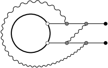
Figure 5: A generally non-planar interaction (left) can become planar when acting on short states (right).

At first sight, it may seem odd to have interactions which depend on the length of the operator. From the point of view of Feynman diagrams this can actually happen: There are structures which are generically non-planar, but can act in a planar fashion on short states. In the notation of [27] the relevant structure is,

$$\mathop{\mathrm{Tr}}\big{[}[\psi_{\alpha},T^{m}],[T^{n},\check{\psi}^{\alpha}]\big{]}\mathop{\mathrm{Tr}}\big{[}[\psi_{\beta},T^{n}],[T^{m},\check{\psi}^{\beta}]\big{]}.$$ (4.17)

For example, this is a crossed two-gluon interaction of two scalar lines, see Fig. 5, left. As the gluon lines are crossed, the interaction is non-planar. However, if the interaction is connected to a state of two fields, one of the gluon lines can be pulled around the state such that it does not cross any of the other lines, see Fig. 5, right. Therefore this interaction is planar exactly for states of length two. This is quite interesting, because it shows that planar physics does have some influence on (generally) non-planar physics.

4.4 Conclusions

We see that for all free parameters in Tab. 1 there is an associated symmetry of the algebra relations and we can say that the two-loop contribution is uniquely fixed. The only parameter that influences energies is $\alpha_{3}$; we cannot remove it by algebraic considerations. The parameters $\gamma_{1,2,3,4}$ rotate only the eigenstates. Finally, the parameters $\delta_{1,2,3}$ are there only because we were not careful enough in finding independent structures (for $H_{4}$ there are only $25=28-3$ independent structures). They have no effect at all.

5 Three-Loop

For the sixth order contributions $H_{6},Q_{4},S_{4}$ we find in total $208+56+56$ parity conserving structures; they all conserve the number of fields. Of these only $173+32+32$ are independent due to identities as discussed in the last section. We imposed the constraint (3.21) at sixth order

$$[Q,\delta H]=[S,\delta H]=\mathcal{O}(g^{7}).$$ (5.1)

and found that the algebra relations fix $202$ coefficients (plus one coefficient at fifth order). This leaves $35$ free coefficients. The anticommutator of supercharges (2.11) at ‘sixth order’

$$\{S^{\alpha}{}_{a},Q^{b}{}_{\beta}\}=\delta^{b}_{a}L^{\alpha}{}_{\beta}+\delta_{\beta}^{\alpha}R^{b}{}_{a}+\delta_{a}^{b}\delta_{\beta}^{\alpha}({\textstyle\frac{1}{3}}H+{\textstyle\frac{1}{6}}\delta H)+\mathcal{O}(g^{5})$$ (5.2)

is satisfied automatically.

As we have learned above, the commutators at sixth order are not enough to ensure consistency for splitting multiplets at the unitarity bound, we should also consider seventh order. To preform those commutators would be even harder. We therefore consider a set of test multiplets at the unitarity bound. By requiring that the three-loop energy shifts coincide within submultiplets we are able to fix another $8$ coefficients.

Still this leaves $27$ coefficients to be fixed, however, almost all of them rotate the space of states. Experimentally, we found that only $4$ coefficients affect the energies. The remaining $23$ coefficients can be attributed to similarity transformations. As before, the number of similarity transformations equals the number of structures for $H_{4}$, i.e. $25$. This means that there must be $2$ commuting generators which are readily found to be $g^{4}H_{2}$ and $g^{4}L$. We summarise our findings concerning the number of coefficients in Tab. 2. The symmetries indicated in the table refer to $L$ (which is conserved at second order but broken at third order, hence the $-1$ at $k=3$), $g^{2}L$ (broken at fifth order), $\delta H$, $g^{4}L$ (will break at seventh order) and $g^{2}\delta H$. This sequence of symmetries will continue at higher orders, but there will be additional ones due to integrability (see Sec. 6.3): Although the second integrable charge acts on three fields and commutes with $H_{2}$, it does not appear here, because it is parity odd. The third charge is parity even and acts on at least four fields. Its commutator with $H_{2}$ vanishes and it will therefore appear at eighth order as one additional symmetry.

$$\begin{array}[]{|c|rrrrr|}\hline\cr k&2&3&4&5&6\\ \hline\cr H_{k}&6&2&25&18&173\\ Q_{k-2}&1&1&4&6&32\\ S_{k-2}&1&1&4&6&32\\ \hline\cr\mbox{total}&8&4&33&30&237\\ \mbox{fixed at $\mathcal{O}(g^{k})$}&5&2&25&26&202\\ \mbox{fixed at $\mathcal{O}(g^{k+1})$}&1&1&3&1&8\\ \mbox{relevant}&1&0&1&0&4\\ \hline\cr\mbox{irrelevant}&1&1&4&3&23\\ \mbox{symmetries}&1&-1&2&-1&2\\ \hline\cr H_{k-2}&2&0&6&2&25\\ \hline\cr\end{array}$$

Table 2: Number of coefficients. $H_{k},Q_{k-2},S_{k-2}$ give the number of independent structures that can be used for the construction of generators. The algebra relations fix a certain number of coefficients. Of the remaining coefficients, some are relevant for energies and some correspond to similarity transformations generated by the structures in $H_{k-2}$. Some of the similarity transformations are symmetries.

Let us now discuss the relevant coefficients. One coefficient is due to a redefinition of the coupling constant and cannot be fixed algebraically. To constrain the other three we will need further input. Unfortunately the resulting generators are too lengthy to be displayed here. Instead, let us have a look at the set of totally bosonic states. In this subsector (which is closed only when further restricted to two flavours, i.e. the $\mathfrak{su}(2)$ subsector) $H_{6}$ is presented in Tab. 3.

$$H_{6}\mathrel{} = \mathrel{}\bigl{(}{\textstyle\frac{15}{2}}\alpha_{1}^{6}+\sigma_{1}-2\sigma_{2}+12\sigma_{3}-2\sigma_{4}+\xi_{2}+\zeta_{1}\bigr{)}\big{\{}{\textstyle\genfrac{}{}{0.0pt}{}{abcd}{abcd}}\big{\}}$$

$$\mathord{}+\bigl{(}-{\textstyle\frac{13}{4}}\alpha_{1}^{6}+\alpha_{1}^{3}\alpha_{3}-{\textstyle\frac{1}{4}}\sigma_{1}+\sigma_{2}-3\sigma_{3}+\sigma_{4}-{\textstyle\frac{1}{2}}\xi_{2}-\zeta_{1}+\zeta_{3}\bigr{)}\bigl{(}\big{\{}{\textstyle\genfrac{}{}{0.0pt}{}{abcd}{abdc}}\big{\}}+\big{\{}{\textstyle\genfrac{}{}{0.0pt}{}{abcd}{bacd}}\big{\}}\bigr{)}$$

$$\mathord{}+\bigl{(}-{\textstyle\frac{13}{2}}\alpha_{1}^{6}+2\alpha_{1}^{3}\alpha_{3}-{\textstyle\frac{1}{2}}\sigma_{1}+2\sigma_{2}-6\sigma_{3}+2\sigma_{4}-\zeta_{1}-\xi_{2}-2\zeta_{3}\bigr{)}\big{\{}{\textstyle\genfrac{}{}{0.0pt}{}{abcd}{acbd}}\big{\}}$$

$$\mathord{}+\bigl{(}{\textstyle\frac{3}{2}}\alpha_{1}^{6}-\alpha_{1}^{3}\alpha_{3}-\sigma_{4}+{\textstyle\frac{1}{2}}\xi_{2}+\zeta_{1}-i\zeta_{2}\bigr{)}\bigl{(}\big{\{}{\textstyle\genfrac{}{}{0.0pt}{}{abcd}{acdb}}\big{\}}+\big{\{}{\textstyle\genfrac{}{}{0.0pt}{}{abcd}{cabd}}\big{\}}\bigr{)}$$

$$\mathord{}+\bigl{(}{\textstyle\frac{3}{2}}\alpha_{1}^{6}-\alpha_{1}^{3}\alpha_{3}-\sigma_{4}+{\textstyle\frac{1}{2}}\xi_{2}+\zeta_{1}+i\zeta_{2}\bigr{)}\bigl{(}\big{\{}{\textstyle\genfrac{}{}{0.0pt}{}{abcd}{adbc}}\big{\}}+\big{\{}{\textstyle\genfrac{}{}{0.0pt}{}{abcd}{bcad}}\big{\}}\bigr{)}$$

$$\mathord{}+\bigl{(}-\sigma_{2}-{\textstyle\frac{1}{2}}\xi_{2}-\zeta_{1}\bigr{)}\bigl{(}\big{\{}{\textstyle\genfrac{}{}{0.0pt}{}{abcd}{adcb}}\big{\}}+\big{\{}{\textstyle\genfrac{}{}{0.0pt}{}{abcd}{cbad}}\big{\}}\bigr{)}+\bigl{(}{\textstyle\frac{1}{2}}\alpha_{1}^{6}-2\sigma_{3}+\zeta_{1}\bigr{)}\big{\{}{\textstyle\genfrac{}{}{0.0pt}{}{abcd}{badc}}\big{\}}$$

$$\mathord{}+\bigl{(}-{\textstyle\frac{1}{2}}\alpha_{1}^{6}+2\sigma_{2}-4\sigma_{3}+2\sigma_{4}-\zeta_{1}\bigr{)}\bigl{(}\big{\{}{\textstyle\genfrac{}{}{0.0pt}{}{abcd}{bcda}}\big{\}}+\big{\{}{\textstyle\genfrac{}{}{0.0pt}{}{abcd}{dabc}}\big{\}}\bigr{)}$$

$$\mathord{}+\bigl{(}-2\sigma_{2}+4\sigma_{3}+\sigma_{4}-i\xi_{3}-\zeta_{1}\bigr{)}\big{\{}{\textstyle\genfrac{}{}{0.0pt}{}{abcd}{bdac}}\big{\}}+\bigl{(}-2\sigma_{2}+4\sigma_{3}+\sigma_{4}+i\xi_{3}-\zeta_{1}\bigr{)}\big{\{}{\textstyle\genfrac{}{}{0.0pt}{}{abcd}{cadb}}\big{\}}$$

$$\mathord{}+\bigl{(}\sigma_{3}-\sigma_{4}+i\xi_{1}+\zeta_{1}\bigr{)}\bigl{(}\big{\{}{\textstyle\genfrac{}{}{0.0pt}{}{abcd}{bdca}}\big{\}}+\big{\{}{\textstyle\genfrac{}{}{0.0pt}{}{abcd}{dbac}}\big{\}}\bigr{)}+\bigl{(}\sigma_{3}-\sigma_{4}-i\xi_{1}+\zeta_{1}\bigr{)}\bigl{(}\big{\{}{\textstyle\genfrac{}{}{0.0pt}{}{abcd}{cbda}}\big{\}}+\big{\{}{\textstyle\genfrac{}{}{0.0pt}{}{abcd}{dacb}}\big{\}}\bigr{)}$$

$$\mathord{}+\bigl{(}-2\sigma_{3}-2\sigma_{4}+\zeta_{1}\bigr{)}\big{\{}{\textstyle\genfrac{}{}{0.0pt}{}{abcd}{cdab}}\big{\}}+\bigl{(}-\zeta_{1}\bigr{)}\bigl{(}\big{\{}{\textstyle\genfrac{}{}{0.0pt}{}{abcd}{cdba}}\big{\}}+\big{\{}{\textstyle\genfrac{}{}{0.0pt}{}{abcd}{dcab}}\big{\}}\bigr{)}$$

$$\mathord{}+\bigl{(}2\sigma_{4}-\zeta_{1}\bigr{)}\big{\{}{\textstyle\genfrac{}{}{0.0pt}{}{abcd}{dbca}}\big{\}}+\bigl{(}\zeta_{1}\bigr{)}\big{\{}{\textstyle\genfrac{}{}{0.0pt}{}{abcd}{dcba}}\big{\}}.$$

Table 3: $H_{6}$ in the bosonic subsector.

The coefficients in Tab. 3 can be understood as follows. The coefficients $\sigma_{1,2,3,4}$ are relevant. One of them, $\sigma_{1}$, multiplies the structure $H_{2}$ (up to spectator legs (3.6)) and therefore corresponds to a redefinition of the coupling constant as in (4.9). The coefficients $\zeta_{1,2,3}$ multiply structures which are actually zero, more explicitly, $\zeta_{1}$ multiplies $\big{\{}{\textstyle\genfrac{}{}{0.0pt}{}{abcd}{[abcd]}}\big{\}}$ and $\zeta_{2,3}$ can be gauged away using (3.6). Finally, the coefficients $\xi_{1,2,3}$ are related to similarity transformations and have no effect of the energy shifts.

The crucial point is that we want $H_{6}$ to be generated by Feynman diagrams. Here we can make use of a special property of the scalar sector. The Feynman diagrams with the maximum number of eight legs do not have internal index loops. In the planar case, such diagrams are iterated one-loop diagrams. This means that we can only have three permutations of adjacent fields. The structures

$$\big{\{}{\textstyle\genfrac{}{}{0.0pt}{}{abcd}{cdab}}\big{\}},\big{\{}{\textstyle\genfrac{}{}{0.0pt}{}{abcd}{bdca}}\big{\}},\big{\{}{\textstyle\genfrac{}{}{0.0pt}{}{abcd}{dbac}}\big{\}},\big{\{}{\textstyle\genfrac{}{}{0.0pt}{}{abcd}{cbda}}\big{\}},\big{\{}{\textstyle\genfrac{}{}{0.0pt}{}{abcd}{dacb}}\big{\}},\quad\big{\{}{\textstyle\genfrac{}{}{0.0pt}{}{abcd}{cdba}}\big{\}},\big{\{}{\textstyle\genfrac{}{}{0.0pt}{}{abcd}{dcab}}\big{\}},\big{\{}{\textstyle\genfrac{}{}{0.0pt}{}{abcd}{dbca}}\big{\}},\quad\big{\{}{\textstyle\genfrac{}{}{0.0pt}{}{abcd}{dcba}}\big{\}}$$ (5.3)

consist of four, five or six crossings of adjacent fields and are therefore excluded. We must set their coefficients to zero

$$\sigma_{3}=\sigma_{4}=0,\qquad\zeta_{1}=\xi_{1}=0.$$ (5.4)

The final relevant coefficient $\sigma_{2}$ multiplies a structure $\mathcal{Q}_{3,0}$ which commutes with $H_{2}=\mathcal{Q}_{2,0}$. At this point we cannot determine $\sigma_{2}$, but believe that it might be fixed due to the anticommutator (2.11) $\{Q,S\}$ at $\mathcal{O}(g^{6})$ (four loops), see Sec. 6.3.

6 The Spectrum and Integrability

In this section we fix the remaining degrees of freedom within $H$ and apply it to find the energy shifts of the first few states in the spectrum.

6.1 The Remaining Coefficients

First of all, we would like to fix the remaining relevant coefficients. We cannot do this algebraically, because they correspond to symmetries of the commutation relations, namely a redefinition of the coupling constant

$$g\mapsto f(g).$$ (6.1)

Unlike the other symmetries, it has relevant consequences, it implies that energies are changed according to

$$E(g)\mapsto E(f(g)).$$ (6.2)

In order to match these degrees of freedom to $\mathcal{N}=4$ SYM we should use some scaling dimension that is known to all orders in perturbation theory. Namely in the planar BMN limit [6] precise all-orders results for gauge theory have been obtained [52, 53]. In fact it is sufficient to use the scaling behaviour for BMN states, their energies should depend only on

$$\lambda^{\prime}=\frac{\lambda}{J^{2}}.$$ (6.3)

If we redefine the coupling constant $g\sim\sqrt{\lambda}$ we obtain for $\lambda^{\prime}$

$$\lambda^{\prime}\mapsto\frac{\tilde{f}(\lambda)}{J^{2}}=\frac{\tilde{f}_{1}\lambda+\tilde{f}_{2}\lambda^{2}+\ldots}{J^{2}}=\tilde{f}_{1}\lambda^{\prime}+\tilde{f}_{2}\lambda^{\prime\,2}J^{2}+\ldots\,\,.$$ (6.4)

The problem is that all the higher expansion coefficients of $\tilde{f}$ yield divergent contributions in the BMN limit $J\to\infty$

$$\frac{\tilde{f}_{k}\lambda^{k}}{J^{2}}=\tilde{f}_{k}\lambda^{\prime\,k}J^{2k-2}\to\infty\qquad\mbox{for }k\neq 1,$$ (6.5)

and the only degree of freedom compatible with the BMN limit is to rescale $\lambda$ by a factor $\tilde{f}_{1}$. In our model we must define the coupling constant $g\sim\sqrt{\lambda}$ in such a way as to obtain good scaling behaviour of energies in the BMN limit. This fixes $\alpha_{3},\sigma_{1}$ and, gladly, also the single coefficient at three-loops that could not be determined, $\sigma_{2}$

$$\alpha_{3}=0,\quad\sigma_{1}=0,\quad\sigma_{2}=0.$$ (6.6)

After that we can only rescale $\alpha_{1}$. This final degree of freedom is eliminated by knowing a single scaling dimension, e.g. the one of the Konishi multiplet [62, 63, 64] $\delta D=3g_{\scriptscriptstyle\mathrm{YM}}^{2}N/4\pi^{4}$, or using the quantitative BMN energy formula [6]. We now define

$$g^{2}=\frac{g_{\scriptscriptstyle\mathrm{YM}}^{2}N}{8\pi^{2}}$$ (6.7)

this fixes $\alpha_{1}$ to unity

$$\alpha_{1}=1.$$ (6.8)

We conclude that the planar three-loop Hamiltonian is uniquely fixed by the symmetry algebra, field theory and the BMN limit. Together with the fact that this model is a closed subsector of $\mathcal{N}=4$ SYM [21] we have thus derived the dilatation generator in the $\mathfrak{su}(2|3)$ subsector at three-loops. Similarly, this model is a closed subsector of the BMN matrix model and the two Hamiltonians must agree up to three loops (after a redefinition of the coupling constant and provided that the BMN matrix model has a BMN limit). Some comments:

• We confirm the three-loop results of [27, 56]. These are restricted to the $\mathfrak{su}(2)$ subsector. Here, we have extended the analysis to the $\mathfrak{su}(2|3)$ subsector.

• The three-loop contribution in [27] is based on the assumption of higher-loop integrability. Here, we relied only on established facts of gauge theory and can thus actually derive integrability, see Sec. 6.3.

• The symmetry algebra $\mathfrak{su}(2|3)$ constrains the number of independent coefficients considerably more than $\mathfrak{su}(2)$. As opposed to $3$ (two-loop) and $6$ (three-loop) coefficients in the $\mathfrak{su}(2)$ subsector we find only $1$ and $2$ here. It may be hoped for that the full symmetry algebra of $\mathcal{N}=4$ SYM, $\mathfrak{psu}(2,2|4)$, fixes the coefficients uniquely to all orders.

• Our result does not agree with a recent result of near plane wave string theory [51]. One will have to think how to make the near-BMN correspondence work in this case.

6.2 Spectrum

We are now ready to compute numerical values for some energy shifts. For this we should consider the charges $E_{0},s,p,q,L$ of a state and compute its constituents according to (2.16). These are arranged within a trace in all possible ways

$$\mathcal{O}_{n}=(\mathop{\mathrm{Tr}}\phi_{1}^{n_{1}}\phi_{2}^{n_{2}}\phi_{3}^{n_{3}}\psi_{1}^{n_{4}}\psi_{2}^{n_{5}},\ldots).$$ (6.9)

Note that the length $L$ is not a good quantum number at $\mathcal{O}(g_{\scriptscriptstyle\mathrm{YM}}^{3})$, so we must include states of all admissible lengths in (6.9). In practice this means that we may replace a complete set of bosons $\phi_{1}\phi_{2}\phi_{3}$ by a complete set of fermions $\psi_{1}\psi_{2}$, (2.24). Due to conservation of charges the Hamiltonian closes on this set of states and we can evaluate its matrix elements

$$H(g)\,\mathcal{O}_{n}=H_{n}{}^{m}(g)\,\mathcal{O}_{m}.$$ (6.10)

It is a straightforward task to find the eigenvalues and their perturbations. By construction the $\mathcal{O}(g^{0})$ eigenvalue $E_{0}$ is universal for all states $\mathcal{O}_{n}$ and perturbation theory will start at $\mathcal{O}(g^{2})$

$$H(g)=E_{0}+g^{2}\left(h+V(g)\right),\qquad\mbox{with }V=\mathcal{O}(g).$$ (6.11)

Diagonalising the leading order matrix $h$ is a non-linear problem. The resulting eigenvalues represent the one-loop energy shifts $\delta E_{2}$. Now we pick an eigenvalue $e$ of $h$ and consider the subspace of states with one-loop energy shift $\delta E_{2}=e$. The higher-order energy shifts are given by (in contrast to the results of [56] $V^{\prime}$ was constructed such that conjugation symmetry is preserved)

$$V^{\prime}\mathrel{} = \mathrel{}\smash{\sum\nolimits_{e}\mathnormal{\Pi}_{e}\Big{[}}V+V\mathnormal{\Delta}_{e}V+\bigl{(}V\mathnormal{\Delta}_{e}V\mathnormal{\Delta}_{e}V-{\textstyle\frac{1}{2}}V\mathnormal{\Delta}_{e}^{2}V\mathnormal{\Pi}_{e}V-{\textstyle\frac{1}{2}}V\mathnormal{\Pi}_{e}V\mathnormal{\Delta}^{2}_{e}V\bigr{)}$$

$$\mathord{}\qquad\qquad+V\mathnormal{\Delta}_{e}V\mathnormal{\Delta}_{e}V\mathnormal{\Delta}_{e}V-{\textstyle\frac{1}{2}}V\mathnormal{\Delta}_{e}^{2}V\mathnormal{\Pi}_{e}V\mathnormal{\Delta}_{e}V-{\textstyle\frac{1}{2}}V\mathnormal{\Delta}_{e}V\mathnormal{\Pi}_{e}V\mathnormal{\Delta}_{e}^{2}V$$

$$\mathord{}\qquad\qquad-{\textstyle\frac{1}{2}}V\mathnormal{\Delta}_{e}^{2}V\mathnormal{\Delta}_{e}V\mathnormal{\Pi}_{e}V-{\textstyle\frac{1}{2}}V\mathnormal{\Pi}_{e}V\mathnormal{\Delta}_{e}V\mathnormal{\Delta}_{e}^{2}V$$

$$\mathord{}\qquad\qquad-{\textstyle\frac{1}{2}}V\mathnormal{\Delta}_{e}V\mathnormal{\Delta}_{e}^{2}V\mathnormal{\Pi}_{e}V-{\textstyle\frac{1}{2}}V\mathnormal{\Pi}_{e}V\mathnormal{\Delta}_{e}^{2}V\mathnormal{\Delta}_{e}V$$

$$\mathord{}\qquad\qquad+{\textstyle\frac{1}{3}}V\mathnormal{\Delta}_{e}^{3}V\mathnormal{\Pi}_{e}V\mathnormal{\Pi}_{e}V+{\textstyle\frac{1}{3}}V\mathnormal{\Pi}_{e}V\mathnormal{\Delta}_{e}^{3}V\mathnormal{\Pi}_{e}V+{\textstyle\frac{1}{3}}V\mathnormal{\Pi}_{e}V\mathnormal{\Pi}_{e}V\mathnormal{\Delta}_{e}^{3}V+\ldots\smash{\Big{]}}\mathnormal{\Pi}_{e}.$$

The propagator $\mathnormal{\Delta}_{e}$ is given by

$$\mathnormal{\Delta}_{e}=\frac{1-\mathnormal{\Pi}_{e}}{e-h}$$ (6.13)

and $\mathnormal{\Pi}_{e}$ projects to the subspace with leading correction $e$. If there is only a single state with one-loop energy shift $e$, (6.2) gives its higher order corrections. For degenerate states at one-loop, (6.11),(6.2) must be applied iteratively until the resulting matrix $V^{\prime}$ becomes diagonal.

Next, it is important to know the multiplets of states. In the interacting theory there are two types of single-trace multiplets, half-BPS and long ones. The half-BPS multiplets are easily identified, there is one multiplet with labels

$$E=E_{0}=L=p,\quad[0;0;0,p],\quad P=(-1)^{p}$$ (6.14)

for each $p$, they receive no corrections to their energy. Long multiplets are not so easy to find. By means of a C++ computer programme we explicitly constructed the spectrum of all states (up to some energy bound) and iteratively removed the multiplets corresponding to the leftover highest weight state (this ‘sieve’ algorithm, also reminiscent of the standard algorithm for division, is described in more detail in [60, 61]). For a set of states with given charges as in (6.9) this also tells us how many representatives there are from each of the multiplets and allows us to identify the energy shift we are interested in.

Finally, to obtain the energy shift of a given multiplet, a lot of work can be saved by choosing a suitable representative. Resolving the mixing problem for the highest weight state is usually more involved than for a descendant. For instance, highest weight states involve all three flavours of bosons, $n_{1},n_{2},n_{3}\geq 1$. This increases the number of permutations in (6.9) and also gives rise to mixing between states of different lengths. The matrix $H_{n}{}^{m}$ (6.10) will be unnecessarily large. If, instead, one applies three supergenerators $Q^{1}{}_{4}Q^{2}{}_{4}Q^{3}{}_{4}$, i.e.

$$n_{1}\mapsto n_{1}-1,\quad n_{2}\mapsto n_{2}-1,\quad n_{3}\mapsto n_{3}-1,\quad n_{4}\mapsto n_{4}+3,$$ (6.15)

the state becomes more uniform. This decreases the number of permutations and, in the case of multiplets at the unitarity bound (2.18), mixing between states of different lengths is prevented due to $n_{3}=0$.

$\begin{array}[]{|l|lc|l|}\hline\cr E_{0}&\lx@intercol\hfil\mathfrak{su}(2|3)\hfil\lx@intercol&L&\bigl{(}\delta E_{2},-\delta E_{4},\delta E_{6}\bigr{)}^{P}\\ \hline\cr 2&[0;0;0,2]^{\dagger\bullet}&2&(0,0,0)^{+}\\ \hline\cr 3&[0;0;0,3]^{\dagger\bullet}&3&(0,0,0)^{-}\\ 3&[0;1;0,0]^{\ast\bullet}&3&\bigl{(}6,12,42\bigr{)}^{+}\\ \hline\cr 4&[0;0;0,4]^{\dagger\bullet}&4&(0,0,0)^{+}\\ 4&[0;1;0,1]^{\ast\bullet}&4&\bigl{(}4,6,17\bigr{)}^{-}\\ \hline\cr 5&[0;0;0,5]^{\dagger\bullet}&5&(0,0,0)^{-}\\ 5&[0;1;0,2]^{\ast\bullet}&5&\bigl{(}10\omega-20,17\omega-60,\frac{117}{2}\omega-230\bigr{)}^{+}\\ 5&[0;1;1,0]^{\ast\bullet}&5&\bigl{(}6,9,\frac{63}{2}\bigr{)}^{-}\\ \hline\cr 6&[0;0;0,6]^{\dagger\bullet}&6&(0,0,0)^{+}\\ 6&[0;1;0,3]^{\ast\bullet}&6&\bigl{(}2,\frac{3}{2},\frac{37}{16}\bigr{)}^{-},\bigl{(}6,\frac{21}{2},\frac{555}{16}\bigr{)}^{-}\\ 6&[0;1;1,1]^{\ast\bullet}&6&\bigl{(}5,\frac{15}{2},25\bigr{)}^{\pm}\\ 6&[0;2;0,0]&6&\bigl{(}14\omega-36,24\omega-90,\frac{173}{2}\omega-315\bigr{)}^{+}\\ 6&[2;3;0,0]^{\ast}&5&\bigl{(}10,20,\frac{145}{2}\bigr{)}^{-}\\ \hline\cr 6.5&[1;2;0,2]^{\ast}&6&\bigl{(}8,14,49\bigr{)}^{\pm}\\ \hline\cr 7&[0;0;0,7]^{\dagger\bullet}&7&\bigl{(}0,0,0\bigr{)}^{-}\\ 7&[0;1;0,4]^{\ast\bullet}&7&\bigl{(}\scriptstyle 14\omega^{2}-56\omega+56,\,23\omega^{2}-172\omega+224,\,79\omega^{2}-695\omega+966\bigr{)}^{+}\\ 7&[0;1;1,2]^{\ast\bullet}&7&\bigl{(}4,5,14\bigr{)}^{\pm},\bigl{(}6,9,33\bigr{)}^{-}\\ 7&[0;1;2,0]^{\ast\bullet}&7&\bigl{(}\scriptstyle 20\omega^{2}-116\omega+200,\,32\omega^{2}-340\omega+800,\,112\omega^{2}-1400\omega+3600\bigr{)}^{+}\\ 7&[0;2;0,1]&7&\bigl{(}\scriptstyle 22\omega^{2}-144\omega+248,\,37\omega^{2}-460\omega+1016,\,125\omega^{2}-1893\omega+4438\bigr{)}^{-}\\ 7&[2;3;0,1]^{\ast}&6&\bigl{(}8,14,46\bigr{)}^{+}\\ \hline\cr 7.5&[1;2;0,3]^{\ast}&7&\bigl{(}7,12,\frac{83}{2}\bigr{)}^{\pm}\\ 7.5&[1;2;1,1]^{\ast}&7&\bigl{(}6,\frac{33}{4},\frac{1557}{64}\bigr{)}^{\pm},\bigl{(}10,\frac{75}{4},\frac{4315}{64}\bigr{)}^{\pm}\\ 7.5&[1;3;0,0]&7&\bigl{(}9,15,51\bigr{)}^{\pm}\\ \hline\cr 8&[0;0;0,8]^{\dagger\bullet}&8&\bigl{(}0,0,0\bigr{)}^{+}\\ 8&[0;1;0,5]^{\ast\bullet}&8&\bigl{(}4,5,\frac{49}{4}\bigr{)}^{-},\bigl{(}8\omega-8,13\omega-18,\frac{179}{4}\omega-61\bigr{)}^{-}\\ 8&[0;1;1,3]^{\ast\bullet}&8&\bigl{(}\scriptstyle 17\omega^{2}-90\omega+147,\,\frac{51}{2}\omega^{2}-\frac{525}{2}\omega+\frac{1239}{2},\,\frac{169}{2}\omega^{2}-\frac{2091}{2}\omega+\frac{5649}{2}\bigr{)}^{\pm}\\ 8&[0;1;2,1]^{\ast\bullet}&8&\bigl{(}5,\frac{15}{2},\frac{55}{2}\bigr{)}^{\pm},\bigl{(}12\omega-24,18\omega-54,57\omega-171\bigr{)}^{-}\\ 8&[0;2;0,2]&8&\bigl{(}7,\frac{19}{2},\frac{59}{2}\bigr{)}^{\pm},\bigl{(}\scriptstyle 44\omega^{5}-768\omega^{4}+6752\omega^{3}-31168\omega^{2}+70528\omega-60224,\,A,\,B\bigr{)}^{+}\\ 8&[0;2;1,0]&8&\bigl{(}9,\frac{31}{2},\frac{103}{2}\bigr{)}^{\pm},\bigl{(}\scriptstyle 24\omega^{2}-172\omega+344,\,39\omega^{2}-524\omega+1372,\,138\omega^{2}-2209\omega+6198\bigr{)}^{-}\\ 8&[2;3;0,2]^{\ast}&7&\bigl{(}\scriptstyle 28\omega^{2}-252\omega+728,\,51\omega^{2}-906\omega+3864,\,179\omega^{2}-3965\omega+20090\bigr{)}^{-}\\ 8&[2;3;1,0]^{\ast}&7&\bigl{(}8,\frac{25}{2},\frac{687}{16}\bigr{)}^{+},\bigl{(}12,\frac{45}{2},\frac{1281}{16}\bigr{)}^{+}\\ \hline\cr 8.5&[1;2;0,4]^{\ast}&8&\bigl{(}6,\frac{19}{2},\frac{247}{8}\bigr{)}^{\pm},\bigl{(}8,\frac{29}{2},\frac{427}{8}\bigr{)}^{\pm}\\ 8.5&[1;2;1,2]^{\ast}&8&\bigl{(}\scriptstyle 31\omega^{3}-350\omega^{2}+1704\omega-3016,\,50\omega^{3}-1111\omega^{2}+7971\omega-18452,\,C\bigr{)}^{\pm}\\ 8.5&[1;2;2,0]^{\ast}&8&\bigl{(}8,13,\frac{343}{8}\bigr{)}^{\pm},\bigl{(}15\omega-48,23\omega-135,\frac{595}{8}\omega-\frac{4023}{8}\bigr{)}^{\pm}\\ 8.5&[1;3;0,1]&8&\bigl{(}8,13,\frac{173}{4}\bigr{)}^{\pm},\bigl{(}10,\frac{67}{4},\frac{3725}{64}\bigr{)}^{\pm},\bigl{(}\scriptstyle 19\omega-86,\,\frac{133}{4}\omega-\frac{1169}{4},\,\frac{7395}{64}\omega-\frac{79503}{64}\bigr{)}^{\pm}\\ \hline\cr\end{array}$

$$A\mathrel{} = \mathrel{}73\omega^{5}-2486\omega^{4}+31804\omega^{3}-188280\omega^{2}+506048\omega-487104\omega$$

$$B\mathrel{} = \mathrel{}251\omega^{5}-10452\omega^{4}+156202\omega^{3}-1041992\omega^{2}+3055168\omega-3125328$$

$$C\mathrel{} = \mathrel{}\textstyle\frac{337}{2}\omega^{3}-\frac{18363}{4}\omega^{2}+38740\omega-102390$$

Table 4: Spectrum of highest weight states with $E_{0}\leq 8.5$ in the dynamic $\mathfrak{su}(2|3)$ spin chain.

We summarise our findings for states of classical energy $E_{0}\leq 8.5$ in Tab. 4. We have labelled the states by their classical energy $E_{0}$, $\mathfrak{su}(2|3)$ Dynkin labels, and classical length $L$. For each multiplet we have given its energy shifts $\delta E=g^{2}\delta E_{2}+g^{4}\delta E_{4}+g^{6}\delta E_{6}+\mathcal{O}(g^{8})$ up to three-loops (note that the two-loop energy shift is always negative, we present its absolute value) and parity $P$. A pair of degenerate states with opposite parity is labelled by $P=\pm$. For convenience we have indicated the shortening conditions relevant for the $\mathfrak{su}(2|3)$ representations: Half-BPS multiplets and multiplets at the unitarity bound (which split at $g=0$) are labelled by ^† and ^∗, respectively. For $s=0$ some of their components are in the $\mathfrak{su}(2)$ subsector. Such multiplets are indicated by ^∙ and their energy shifts agree with the results of [27].

Generically, the one-loop energy shifts are not fractional numbers but solutions to some algebraic equations. We refrain from solving them (numerically), but instead give the equations. In the table such states are indicated as polynomials $\delta E_{2,4,6}(\omega)$ of degree $k-1$ (note that the table shows $-\delta E_{4}(\omega)$). The energy shifts are obtained as solutions to the equation

$$\delta E=g^{2}\,\omega,\qquad\omega^{k}=\delta E_{2}(\omega)+g^{2}\,\delta E_{4}(\omega)+g^{4}\,\delta E_{6}(\omega)+\mathcal{O}(g^{6}).$$ (6.16)

6.3 Integrability

A closer look at Tab. 4 shows that there is a maximum amount of parity pairs. All multiplets with opposite parities which can pair up, actually do have degenerate energies. At the one-loop level, where the Hamiltonian is the Hamiltonian of a classical integrable $\mathfrak{su}(2|3)$ spin chain, this is explained by integrability [27]. For an integrable spin chain one can construct a transfer operator $\mathcal{T}_{0}(u)$ satisfying

$$[J_{0},\mathcal{T}_{0}(u)]=[\mathcal{T}_{0}(u),\mathcal{T}_{0}(v)]=0.$$ (6.17)

When expanded in the spectral parameter $u$ the transfer matrix

$$\mathcal{T}_{0}(u)=\exp\sum_{n=2}^{\infty}\frac{u^{n-1}}{(n-1)!}\,\mathcal{Q}_{n,0}$$ (6.18)

gives rise to an infinite tower (for sufficiently long states) of mutually commuting local charges $\mathcal{Q}_{n,0}$,

$$[J_{0},\mathcal{Q}_{n,0}]=[\mathcal{Q}_{m,0},\mathcal{Q}_{n,0}]=0.$$ (6.19)

The charge $\mathcal{Q}_{n,0}$ extends over $n$ nearest neighbours and has parity $(-1)^{n}$. The one-loop Hamiltonian is the first non-trivial of these $H_{2}=\mathcal{Q}_{2,0}$. The second non-trivial charge, $\mathcal{Q}_{3,0}$, is parity odd and its action relates states of opposite parity

$$\mathcal{Q}_{3,0}\,\mathcal{O}_{\pm}\sim\mathcal{O}_{\mp}.$$ (6.20)

Its conservation implies the degeneracy of $\mathcal{O}_{\pm}$. In the classical spin chain this is only valid at one-loop, but here we notice that energy shifts do agree within pairs to the order we are investigating. As shown in [27] this can be explained by an extension of the higher charges $\mathcal{Q}_{n,0}$ to higher loops

$$\mathcal{Q}_{n}(g)=\sum_{k=0}^{\infty}g^{k}\,\mathcal{Q}_{n,k},$$ (6.21)

where $\mathcal{Q}_{n,k}$ is a local interaction with $2n+k$ legs (incoming plus outgoing fields). Higher-loop integrability demands that the charges commute among themselves (in a perturbative sense)

$$[J(g),\mathcal{Q}_{n}(g)]=[\mathcal{Q}_{m}(g),\mathcal{Q}_{n}(g)]=0$$ (6.22)

or in terms of a higher-loop transfer operator

$$\mathcal{T}(u,g)=\sum_{k=0}^{\infty}g^{k}\,\mathcal{T}_{k}(u)=\exp\sum_{n=2}^{\infty}\sum_{k=0}^{\infty}\frac{u^{n-1}}{(n-1)!}\,g^{k}\,\mathcal{Q}_{n,k}$$ (6.23)

with

$$[J(g),\mathcal{T}(u,g)]=[\mathcal{T}(u,g),\mathcal{T}(v,g)]=0.$$ (6.24)

Moreover, in analogy to (3.19), we should demand that the charges have zero classical energy

$$[H_{0},\mathcal{Q}_{n}(g)]=[H_{0},\mathcal{T}(u,g)]=0.$$ (6.25)

From (6.22) it follows that the energy shift $\delta H(g)$ commutes with the charges

$$[\delta H(g),\mathcal{Q}_{n}(g)]=[\delta H(g),\mathcal{T}(u,g)]=0.$$ (6.26)

Here we did not construct any higher charges, but note that all possible pairs (^±) remain degenerate at three-loops. This is so for the pairs of the $\mathfrak{su}(2)$ sector (^∙) [27], for pairs at the unitarity bound (^∗), but also, and most importantly, for pairs away from the unitarity bound (unmarked in Tab. 4). As discussed at the end of Sec. 2.3 all states of such a multiplet are superpositions of states of different lengths. We take this as compelling evidence for the existence of higher charges $\mathcal{Q}_{n}(g)$ . This is interesting, because it shows that also for truly dynamic spin chains with a fluctuating number of sites integrability is an option.

Let us now comment on the rôle of the interaction Hamiltonian $\delta H(g)$. On the one hand it belongs to the symmetry algebra $\mathfrak{su}(2|3)$ when combined with $H_{0}$ (see footnote 6 on page 6)

$$H(g)+{\textstyle\frac{1}{2}}\delta H(g)=H_{0}+{\textstyle\frac{3}{2}}\delta H(g)\in\mathfrak{su}(2|3).$$ (6.27)

On the other hand (6.26), together with $[J(g),\delta H(g)]=0$ (3.21), shows that $\delta H(g)$ is also a generator of the abelian algebra of local integrable charges $\mathbb{R}^{\infty}$ defined by (6.22)

$$g^{-2}\,\delta H(g)\in\mathbb{R}^{\infty}.$$ (6.28)

At this point we can reinvestigate the undetermined coefficients at three-loops. By imposing

$$[Q(g),\delta H(g)]=[S(g),\delta H(g)]=\mathcal{O}(g^{8})$$ (6.29)

we found that $H_{6}$ depends on four relevant coefficients $\sigma_{1,2,3,4}$. The coefficients $\sigma_{3,4}$ multiply invalid structures, whereas $\sigma_{1}$ corresponds to a redefinition of the coupling constant. The remaining coefficient $\sigma_{2}$ multiplies $\mathcal{Q}_{4,0}$ which is structurally equivalent to $H_{6}$ and satisfies $[J(g),\mathcal{Q}_{4}(g)]=0$ as well. In fact, by imposing $[Q(g),X(g)]=[S(g),X(g)]=0$ we not only find $\delta H$, but also all the other even generators $\mathcal{Q}_{2n}(g)$ of the abelian algebra of integrable charges $\mathbb{R}^{\infty}$. Thus $\sigma_{2}$ corresponds to the transformation

$$\delta H(g)\mapsto\delta H(g)+\sigma_{2}\,g^{6}\,\mathcal{Q}_{4}(g),$$ (6.30)

which has no influence on (6.29) due to $[J(g),\mathcal{Q}_{n}(g)]=0$. This degree of freedom may be fixed by considering the anticommutator of supercharges (2.11)

$$\{S^{\alpha}{}_{a}(g),Q^{b}{}_{\beta}(g)\}=\delta^{b}_{a}L^{\alpha}{}_{\beta}+\delta_{\beta}^{\alpha}R^{b}{}_{a}+\delta_{a}^{b}\delta_{\beta}^{\alpha}\bigl{(}{\textstyle\frac{1}{3}}H_{0}+{\textstyle\frac{1}{2}}\delta H(g)\bigr{)}+\mathcal{O}(g^{7}).$$ (6.31)

Unfortunately this involves $Q_{6},S_{6}$ which are part of a four-loop calculation and out of reach here. We believe that (6.31) will force the coefficient $\sigma_{2}$ to vanish, and in conclusion all corrections up to three loops would be determined uniquely (up to a redefinition of the coupling constant). At higher loops this picture is expected to continue: While $[Q(g),X(g)]=[S(g),X(g)]=0$ determines elements $\mathcal{Q}_{2n}$ of $\mathbb{R}^{\infty}$, the anticommutator $\{S(g),Q(g)\}$ yields the one element $\delta H(g)$ (6.28) which is also associated to $\mathfrak{su}(2|3)$ via (6.27).

Let us comment on the uniqueness of the $n$-th charge $\mathcal{Q}_{n}$. As the charges form an abelian algebra, one can replace $\mathcal{Q}_{n}$ by some polynomial in the charges without changing the algebra. This, however, would make $\mathcal{Q}_{n}$ multi-local in general. To preserve locality we must use linear transformations which are generated by

$$\mathcal{Q}_{n}(g)\mapsto\mathcal{Q}_{n}(g)+\alpha\,g^{2k}\,\mathcal{Q}_{n+2m}(g).$$ (6.32)

On the one hand, the structural constraint on $\mathcal{Q}_{n}$, i.e. that $\mathcal{Q}_{n}$ has at least as many legs as $g^{2k}\mathcal{Q}_{n+2m}$, requires $k\geq 2m$. On the other hand, it was observed that $\mathcal{Q}_{n,k}$ scales as $\mathcal{O}(L^{-k-n})$ in the thermodynamic/BMN limit $L\to\infty$ [32]

$$\mathcal{Q}^{\prime}_{n,k}=\lim_{L\to\infty}L^{k+n}\mathcal{Q}_{n,k}\quad\mbox{or}\quad\mathcal{T}^{\prime}(u^{\prime},g^{\prime})=\lim_{L\to\infty}\mathcal{T}(Lu^{\prime},Lg^{\prime})^{L}$$ (6.33)

In order not to spoil this, we need $k\leq m$. Together, these two constraints imply $k=m=0$, or, in other words, $\mathcal{Q}_{k}$ can only be rescaled by a constant. Finally, this constant can be fixed by using the standard transfer matrix $\mathcal{T}_{0}(u)$ of the one-loop spin-chain, i.e. there is a canonical definition for $\mathcal{Q}_{n}(g)$. As $g^{-2}\delta H(g)$ obeys the same constraints as $\mathcal{Q}_{2}(g)$, both of them must be equal

$$g^{-2}\,\delta H(g)=\mathcal{Q}_{2}(g).$$ (6.34)

The thermodynamic constraint does not allow the transformation (6.30) and thus fixes $\sigma_{2}$ as shown in Sec. 6.1 (even if it is expected to be determined at four-loops, see above).

In agreement with the findings of Klose and Plefka [56] we conclude that integrability appears to be a consequence of field theory combined with symmetry and does not depend on the specific model very much. This strongly supports the idea of all-loop integrability in planar $\mathcal{N}=4$ SYM. What is more, the dynamic aspects of higher-loop spin chains appear to be no obstruction.

7 Outlook

In this work we have derived the planar dilatation generator of $\mathcal{N}=4$ SYM in the $\mathfrak{su}(2|3)$ subsector. This is equivalent to the Hamiltonian of a dynamic spin chain where the number of spin sites is allowed to fluctuate. There are a few open questions and some directions for future research.

First of all, one could try to understand the two-loop deformations in Tab. 1 better and find out how they can be constructed from scratch without having to start with the most general structure and subsequently constraining it. Furthermore, it would be good to have some of the higher charges explicitly. Unfortunately, like the three-loop contribution, already the second charge at two-loops is lengthy. A consideration of the non-planar, finite $N$, algebra would also be interesting.

For the derivation of the three-loop result we have made use of the thermodynamic/BMN limit. As explained, this can probably be avoided by going to four-loops. Why does the closure of the algebra together with the structural constraints yield a Hamiltonian $\delta H(g)$ with a good thermodynamic/BMN limit? What about the higher charges $\mathcal{Q}_{n}(g)$?

One might try to rederive the complete one-loop dilatation operator of $\mathcal{N}=4$ gauge theory [21] with these algebraic methods. The closure of the corresponding $\mathfrak{psu}(2,2|4)$ algebra at third order will probably reduce the infinite number of independent coefficients to just one. One could then proceed to two-loops, either in the full $\mathcal{N}=4$ theory or in a subsector with non-compact representations.

It might also be interesting to extend the current analysis to non-perturbative effects like instantons. Possibly the symmetry algebra also puts constraints on these and a direct computation as in [65] might be simplified or even bypassed.

In any case, a better understanding of dynamic spin chains and, even more urgently, an improved notion of higher-loop integrability is required. This might be a key to unravel planar $\mathcal{N}=4$ gauge theory at all loops.

Acknowledgements

The author would like to thank Gleb Arutyunov, Volodya Kazakov, Thomas Klose, Jan Plefka, Arkady Tseytlin and, in particular, Matthias Staudacher for interesting discussions and useful comments. Ich danke der Studienstiftung des deutschen Volkes für die Unterstützung durch ein Promotionsförderungsstipendium.

References

• [1] J. M. Maldacena, “The large N limit of superconformal field theories and supergravity”, Adv. Theor. Math. Phys. 2, 231 (1998), hep-th/9711200.
• [2] E. Witten, “Anti-de Sitter space and holography”, Adv. Theor. Math. Phys. 2, 253 (1998), hep-th/9802150.
• [3] S. S. Gubser, I. R. Klebanov and A. M. Polyakov, “Gauge theory correlators from non-critical string theory”, Phys. Lett. B428, 105 (1998), hep-th/9802109.
• [4] F. Gliozzi, J. Scherk and D. I. Olive, “Supersymmetry, Supergravity theories and the dual spinor model”, Nucl. Phys. B122, 253 (1977).
• [5] L. Brink, J. H. Schwarz and J. Scherk, “Supersymmetric Yang-Mills Theories”, Nucl. Phys. B121, 77 (1977).
• [6] D. Berenstein, J. M. Maldacena and H. Nastase, “Strings in flat space and pp waves from $\mathcal{N}=\mathord{}$4 Super Yang Mills”, JHEP 0204, 013 (2002), hep-th/0202021.
• [7] C. Kristjansen, J. Plefka, G. W. Semenoff and M. Staudacher, “A new double-scaling limit of $\mathcal{N}=\mathord{}$4 super Yang-Mills theory and PP-wave strings”, Nucl. Phys. B643, 3 (2002), hep-th/0205033.
• [8] N. R. Constable, D. Z. Freedman, M. Headrick, S. Minwalla, L. Motl, A. Postnikov and W. Skiba, “PP-wave string interactions from perturbative Yang-Mills theory”, JHEP 0207, 017 (2002), hep-th/0205089.
• [9] N. Beisert, C. Kristjansen, J. Plefka, G. W. Semenoff and M. Staudacher, “BMN correlators and operator mixing in $\mathcal{N}=\mathord{}$4 super Yang-Mills theory”, Nucl. Phys. B650, 125 (2003), hep-th/0208178.
• [10] N. R. Constable, D. Z. Freedman, M. Headrick and S. Minwalla, “Operator mixing and the BMN correspondence”, JHEP 0210, 068 (2002), hep-th/0209002.
• [11] N. Beisert, C. Kristjansen, J. Plefka and M. Staudacher, “BMN gauge theory as a quantum mechanical system”, Phys. Lett. B558, 229 (2003), hep-th/0212269.
• [12] J. A. Minahan and K. Zarembo, “The Bethe-ansatz for $\mathcal{N}=\mathord{}$4 super Yang-Mills”, JHEP 0303, 013 (2003), hep-th/0212208.
• [13] L. N. Lipatov, “High-energy asymptotics of multicolor QCD and exactly solvable lattice models”, JETP Lett. 59, 596 (1994), hep-th/9311037.
• [14] L. D. Faddeev and G. P. Korchemsky, “High-energy QCD as a completely integrable model”, Phys. Lett. B342, 311 (1995), hep-th/9404173.
• [15] V. M. Braun, S. E. Derkachov and A. N. Manashov, “Integrability of three-particle evolution equations in QCD”, Phys. Rev. Lett. 81, 2020 (1998), hep-ph/9805225.
• [16] A. V. Belitsky, “Fine structure of spectrum of twist-three operators in QCD”, Phys. Lett. B453, 59 (1999), hep-ph/9902361.
• [17] V. M. Braun, S. E. Derkachov, G. P. Korchemsky and A. N. Manashov, “Baryon distribution amplitudes in QCD”, Nucl. Phys. B553, 355 (1999), hep-ph/9902375.
• [18] A. V. Belitsky, “Integrability and WKB solution of twist-three evolution equations”, Nucl. Phys. B558, 259 (1999), hep-ph/9903512.
• [19] A. V. Belitsky, “Renormalization of twist-three operators and integrable lattice models”, Nucl. Phys. B574, 407 (2000), hep-ph/9907420.
• [20] S. E. Derkachov, G. P. Korchemsky and A. N. Manashov, “Evolution equations for quark gluon distributions in multi-color QCD and open spin chains”, Nucl. Phys. B566, 203 (2000), hep-ph/9909539.
• [21] N. Beisert, “The Complete One-Loop Dilatation Operator of $\mathcal{N}=\mathord{}$4 Super Yang-Mills Theory”, Nucl. Phys. B676, 3 (2004), hep-th/0307015.
• [22] N. Beisert and M. Staudacher, “The $\mathcal{N}=\mathord{}$4 SYM Integrable Super Spin Chain”, Nucl. Phys. B670, 439 (2003), hep-th/0307042.
• [23] H. Saleur, “The continuum limit of sl(N/K) integrable super spin chains”, Nucl. Phys. B578, 552 (2000), solv-int/9905007.
• [24] A. V. Belitsky, A. S. Gorsky and G. P. Korchemsky, “Gauge/string duality for QCD conformal operators”, Nucl. Phys. B667, 3 (2003), hep-th/0304028.
• [25] L. Dolan, C. R. Nappi and E. Witten, “A Relation Between Approaches to Integrability in Superconformal Yang-Mills Theory”, JHEP 0310, 017 (2003), hep-th/0308089.
• [26] A. Gorsky, “Spin chains and gauge / string duality”, hep-th/0308182.
• [27] N. Beisert, C. Kristjansen and M. Staudacher, “The dilatation operator of $\mathcal{N}=\mathord{}$4 conformal super Yang-Mills theory”, Nucl. Phys. B664, 131 (2003), hep-th/0303060.
• [28] L. D. Faddeev, “How Algebraic Bethe Ansatz works for integrable model”, hep-th/9605187.
• [29] N. Beisert, J. A. Minahan, M. Staudacher and K. Zarembo, “Stringing Spins and Spinning Strings”, JHEP 0309, 010 (2003), hep-th/0306139.
• [30] N. Beisert, S. Frolov, M. Staudacher and A. A. Tseytlin, “Precision Spectroscopy of AdS/CFT”, JHEP 0310, 037 (2003), hep-th/0308117.
• [31] J. Engquist, J. A. Minahan and K. Zarembo, “Yang-Mills Duals for Semiclassical Strings”, hep-th/0310188.
• [32] G. Arutyunov and M. Staudacher, “Matching Higher Conserved Charges for Strings and Spins”, hep-th/0310182.
• [33] S. Frolov and A. A. Tseytlin, “Semiclassical quantization of rotating superstring in $AdS_{5}\times S^{5}$, JHEP 0206, 007 (2002), hep-th/0204226.
• [34] J. G. Russo, “Anomalous dimensions in gauge theories from rotating strings in $AdS_{5}\times S^{5}$, JHEP 0206, 038 (2002), hep-th/0205244.
• [35] J. A. Minahan, “Circular semiclassical string solutions on $AdS_{5}\times S^{5}$, Nucl. Phys. B648, 203 (2003), hep-th/0209047.
• [36] A. A. Tseytlin, “Semiclassical quantization of superstrings: $AdS_{5}\times S^{5}$ and beyond”, Int. J. Mod. Phys. A18, 981 (2003), hep-th/0209116.
• [37] S. Frolov and A. A. Tseytlin, “Multi-spin string solutions in $AdS_{5}\times S^{5}$, Nucl. Phys. B668, 77 (2003), hep-th/0304255.
• [38] S. Frolov and A. A. Tseytlin, “Quantizing three-spin string solution in $AdS_{5}\times S^{5}$, JHEP 0307, 016 (2003), hep-th/0306130.
• [39] S. Frolov and A. A. Tseytlin, “Rotating string solutions: AdS/CFT duality in non-supersymmetric sectors”, Phys. Lett. B570, 96 (2003), hep-th/0306143.
• [40] G. Arutyunov, S. Frolov, J. Russo and A. A. Tseytlin, “Spinning strings in $AdS_{5}\times S^{5}$ and integrable systems”, Nucl. Phys. B671, 3 (2003), hep-th/0307191.
• [41] S. S. Gubser, I. R. Klebanov and A. M. Polyakov, “A semi-classical limit of the gauge/string correspondence”, Nucl. Phys. B636, 99 (2002), hep-th/0204051.
• [42] M. Alishahiha and A. E. Mosaffa, “Circular semiclassical string solutions on confining AdS/CFT backgrounds”, JHEP 0210, 060 (2002), hep-th/0210122.
• [43] M. Alishahiha and A. E. Mosaffa, “Semiclassical string solutions on deformed NS5-brane backgrounds and new pp-wave”, hep-th/0302005.
• [44] D. Mateos, T. Mateos and P. K. Townsend, “Supersymmetry of tensionless rotating strings in $AdS_{5}\times S^{5}$, and nearly-BPS operators”, hep-th/0309114.
• [45] M. Schvellinger, “Spinning and rotating strings for $\mathcal{N}=\mathord{}$1 SYM theory and brane constructions”, hep-th/0309161.
• [46] G. Mandal, N. V. Suryanarayana and S. R. Wadia, “Aspects of semiclassical strings in $AdS_{5}$, Phys. Lett. B543, 81 (2002), hep-th/0206103.
• [47] I. Bena, J. Polchinski and R. Roiban, “Hidden symmetries of the $AdS_{5}\times S^{5}$ superstring”, hep-th/0305116.
• [48] B. C. Vallilo, “Flat Currents in the Classical $AdS_{5}\times S^{5}$ Pure Spinor Superstring”, hep-th/0307018.
• [49] L. F. Alday, “Non-local charges on $AdS_{5}\times S^{5}$ and pp-waves”, hep-th/0310146.
• [50] N. Beisert, “Higher loops, integrability and the near BMN limit”, JHEP 0309, 062 (2003), hep-th/0308074.
• [51] C. G. Callan, Jr., H. K. Lee, T. McLoughlin, J. H. Schwarz, I. Swanson and X. Wu, “Quantizing string theory in $AdS_{5}\times S^{5}$: Beyond the pp-wave”, Nucl. Phys. B673, 3 (2003), hep-th/0307032.
• [52] D. J. Gross, A. Mikhailov and R. Roiban, “Operators with large R charge in $\mathcal{N}=\mathord{}$4 Yang-Mills theory”, Annals Phys. 301, 31 (2002), hep-th/0205066.
• [53] A. Santambrogio and D. Zanon, “Exact anomalous dimensions of $\mathcal{N}=\mathord{}$4 Yang-Mills operators with large R charge”, Phys. Lett. B545, 425 (2002), hep-th/0206079.
• [54] N. Kim and J. Plefka, “On the spectrum of pp-wave matrix theory”, Nucl. Phys. B643, 31 (2002), hep-th/0207034.
• [55] N. Kim, T. Klose and J. Plefka, “Plane-wave Matrix Theory from $\mathcal{N}=\mathord{}$4 Super Yang-Mills on $R\times S^{3}$, Nucl. Phys. B671, 359 (2003), hep-th/0306054.
• [56] T. Klose and J. Plefka, “On the Integrability of large $N$ Plane-Wave Matrix Theory”, hep-th/0310232.
• [57] K. Konishi, “Anomalous supersymmetry transformation of some composite operators in SQCD”, Phys. Lett. B135, 439 (1984).
• [58] K. Konishi and K. Shizuya, “Functional integral approach to chiral anomalies in supersymmetric gauge theories”, Nuovo Cim. A90, 111 (1985).
• [59] B. Eden, “On two fermion BMN operators”, hep-th/0307081.
• [60] M. Bianchi, J. F. Morales and H. Samtleben, “On stringy $AdS_{5}\times S^{5}$ and higher spin holography”, JHEP 0307, 062 (2003), hep-th/0305052.
• [61] N. Beisert, M. Bianchi, J. F. Morales and H. Samtleben, “On the spectrum of AdS/CFT beyond supergravity”, hep-th/0310292.
• [62] D. Anselmi, M. T. Grisaru and A. Johansen, “A Critical Behaviour of Anomalous Currents, Electric-Magnetic Universality and CFT4, Nucl. Phys. B491, 221 (1997), hep-th/9601023.
• [63] D. Anselmi, “The $\mathcal{N}=\mathord{}$4 quantum conformal algebra”, Nucl. Phys. B541, 369 (1999), hep-th/9809192.
• [64] M. Bianchi, S. Kovacs, G. Rossi and Y. S. Stanev, “On the logarithmic behavior in $\mathcal{N}=\mathord{}$4 SYM theory”, JHEP 9908, 020 (1999), hep-th/9906188.
• [65] S. Kovacs, “On instanton contributions to anomalous dimensions in $\mathcal{N}=\mathord{}$4 supersymmetric Yang-Mills theory”, hep-th/0310193.