Similarity renormalization group as a theory of effective particles

Abstract

The similarity renormalization group procedure formulated in terms of effective particles is briefly reviewed in a series of selected examples that range from the model matrix estimates of its numerical accuracy to issues of the Poincaré symmetry in constituent theories to derivation of the Schrödinger equation for quarkonia in QCD.

1 INTRODUCTION

This talk discusses some examples that illustrate recent developments in the effective (constituent) particle approach to quantum field theory (QFT). The new approach followed in the footsteps and emerged from the general renormalization group (RG) procedure for Hamiltonians that uses a similarity transformation [1] instead of a cutoff reduction. Complex issues of small-$x$ dynamics and chiral symmetry that occur in addition to the ultraviolet RG structure in QCD require extended studies and the effective particle picture provides a new framework for them.

2 CUTOFF  $\rightarrow$  BAND WIDTH $\lambda$

Canonical Hamiltonians of local QFTs are plagued by divergences. The divergences stem from the local interactions, which extend over an infinite momentum range and involve unlimited numbers of bare particles. For example, the term $H_{I}=\int d^{3}x\,\bar{\psi}\not A\psi$ produces divergent loop integrals. Therefore, one can ask what is $H_{I}$ to mean in the context of proper quantum mechanics (QM). For example, if already $H_{I}^{2}$ does not exist, why should the evolution operator $\exp{(-iHt)}$ exist? The left drawing on Fig. 1

Figure 1: A bare particle decays into two, or many.

shows a local interaction that turns one particle into two particles whose momenta may be described using standard light-front (LF) variables

$$x_{1}=k_{1}^{+}/k_{3}^{+}\quad,\quad x_{2}=k_{2}^{+}/k_{3}^{+}\quad,\quad\kappa^{\perp}_{12}=x_{2}k^{\perp}_{1}-x_{2}k^{\perp}_{2}\,.$$ (1)

Two cutoffs have to be introduced in $H$ in order to make powers of $H$ and the eigenvalue problem for $H$ finite: $|\kappa^{\perp}|\leq\Lambda$, and $x\geq\delta$. The second cutoff implies that in all interactions the number of annihilated or created particles is limited by $1/\delta$, since all the $x$s must add up to 1 due to translational symmetry. Then, the invariant mass $M^{2}$ of the bare particles in the interaction is limited by $M^{2}\leq\Delta^{2}\sim\Lambda^{2}/\delta$. When the number of particles involved in interactions is limited by $1/\delta$, it also becomes legitimate to restrict the analysis of renormalized theories to polynomial interactions in field variables. But the main point is that instead of thinking in terms of the bare local $H$ itself one needs to think in terms of $H_{\Delta}$ with cutoffs.

Wilson had explained implications of inserting cutoffs into Hamiltonians [2], and he provided a picture of the RG as a family of effective Hamiltonians $H_{\lambda}$, with coupling constants that depend on the scale $\lambda$. For example, the counterterms (CT) in $H_{\Delta}$ can change the coupling constant $g$ to $g+CT_{\Delta}(g)$, a cutoff dependent quantity which is usually denoted by $g_{\Delta}$. In the effective Hamiltonian with a small running cutoff $\lambda$, a similar coupling constant is found, denoted by $g_{\lambda}$. This is illustrated in Fig. 2.

Figure 2: The standard RG procedure with the bare cutoff $\Delta$ and the running cutoff $\lambda$.

But Wilson’s procedure of calculating $H_{\lambda}$ encounters problems with non-trivial interactions across the boundary line at $\lambda$ and with small energy denominators in perturbation theory at the boundary. It becomes very hard to calculate the structure of the CTs in asymptotically free (AF) theories with bound states (BS) where the overlapping divergences cannot be fully controlled unless the BS structure is systematically incorporated in the running of the coupling constants. Thus, it becomes very hard to determine the finite parts of the CTs, control all anomalies, and proceed to a meaningful phenomenological study using a LF Hamiltonian of QCD. The critical issue is that one needs a sufficiently small $\lambda$ so that the memory and CPU requirements in numerical studies become realistic, while small $\lambda$ means that one has to reduce the entire theory dynamics to something small. This is not easy to do in QCD. But the difficulties are partly removed by switching over to the new scheme [1] based on the similarity (most often unitary) transformation, shown in Fig. 3.

Figure 3: The cutoff $\lambda$ is replaced by the width. The zig-zag jumps correspond to perturbation theory (see the original literature).

Beyond this conceptual change, the steps of the RG procedure for calculating CTs remain in principle the same as in the standard RG approach. Note, however, that the genuine infrared divergences due to jumps just across the cutoff boundary in Fig.2 are now entirely removed from the perturbative evaluation of $H_{\lambda}$ in Fig. 3. The differential equation for $H_{\lambda}$ reads (the initial condition at $\lambda=\infty$ is set by $H_{\infty}=H_{\Delta}+CT_{\Delta}$),

$${dH_{\lambda}\over d\lambda}=[T_{\lambda},H_{\lambda}]\,.$$ (2)

$T_{\lambda}$ denotes the generator that needs to be carefully chosen to perform actual calculations.

3 PATH TO 1% ACCURACY

The idea is to define such $T_{\lambda}$ that one can accurately calculate matrix elements in a small window $W_{\lambda}$ (a sub-matrix of the entire Hamiltonian $H_{\lambda}$, see Fig. 4) using perturbation theory,

Figure 4: Small window Hamiltonians $W_{\lambda}$ can be diagonalized using computers.

and then diagonalize the window $W_{\lambda}$ non-perturbatively to produce the masses and wave functions of the BSs in the middle of the energy range covered by the window. An elegant candidate for the generator can be found in Wegner’s flow equation [3]: $T_{\lambda}=[H_{\lambda},H_{0\lambda}]$. A model result obtained using this generator [4] is shown in Fig. 5.

Figure 5: A BS eigenvalue of the window $W_{\lambda}$. The window was calculated in orders $n=1,2,3,4$ of perturbation theory in $g_{\lambda}$ in a matrix model of an AF theory using Wegner’s generator. The exact BS eigenvalue was $E=-1$ GeV.

The failure of the theory to converge for $\lambda<4$ GeV is clearly visible. But when one uses an altered version of $T_{\lambda}$ [4], one is able to obtain Fig. 6, which displays evident signs of stable behavior, and the accuracy of the procedure reaches 1%. In order to take advantage of this apparently powerful method in solving QFT, one can formulate the entire approach in terms of effective particles.

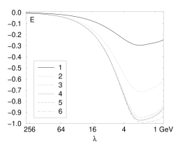
Figure 6: Results from the window $W_{\lambda}$ in the case of the altered Wegner equation, orders 1 to 6, cf. Fig. 5.

4 FROM THE BAND OF WIDTH $\lambda$ TO VERTEX FORM FACTORS $f_{\lambda}$

The RG procedure for effective particles, or RGPEP (early literature on the subject is referenced in [6]) is based on the observation that the initial Hamiltonian $H_{\Delta}$, expressed in terms of bare fields (bare creation and annihilation operators, $q$) can be rewritten in terms of products of creation and annihilation operators for effective particles, $q_{\lambda}$, with new coefficients, so that $H_{\Delta}(q)+CT_{\Delta}(q)=H_{\lambda}(q_{\lambda})$, and

$$q_{\lambda}=U_{\lambda}qU^{\dagger}_{\lambda}\,.$$ (3)

The calculational procedure is designed so that the new coefficient functions in $H_{\lambda}(q_{\lambda})$ allow us to write $H_{\lambda}=f_{\lambda}G_{\lambda}$, where $f_{\lambda}$ denotes the vertex form factors that have momentum-space width $\lambda$, and $G_{\lambda}$ denotes the vertices of the effective interaction terms. The generator $T_{\lambda}$ is chosen so that the interactions evolve with $\lambda$ according to the equation

$$G^{\prime}_{\lambda}=[\{(f_{\lambda}-1)G_{\lambda}\}^{\prime},f_{\lambda}G_{\lambda}]\,.$$ (4)

The form factor $f_{\lambda}$ is a smooth function of the effective particle momenta. It secures that the Hamiltonian $H_{\lambda}$ has non-zero matrix elements only between states whose total invariant masses differ by no more than about $\lambda$.

Although RGPEP is designed for LF QFT, it can also be applied in the matrix model with AF and a BS, which was discussed in the previous section [4]. It turns out that the RGPEP equations can produce results as good as in Fig. 6, i.e., one can calculate the window Hamiltonians $W_{\lambda}$ with accuracy matching the altered Wegner equation. But in addition, the RGPEP in LF dynamics offers a boost invariant formalism that preserves the cluster property of QFT [5] and introduces a dynamical connection between the pointlike partons and effective constituent particles of size $\sim 1/\lambda$.

5 RGPEP IN QFT

Let me observe first that RGPEP explains the phenomenon of AF through dependence of $H_{LF\,QCD\,\lambda}$ on $\lambda$. For example [6], the three-gluon coupling term ($Y_{123}$ is a polarization dependent factor),

$$H_{I\lambda} = \int[123]\,r(x_{1})r(x_{2})\,f_{\lambda}({\cal M}_{12}^{2},{\cal M}_{3}^{2})\,\,V_{\lambda}(\kappa^{\perp}_{12},x_{1})\,Y_{123}\,\,q^{\dagger}_{\lambda 1}q^{\dagger}_{\lambda 2}q_{\lambda 3}\,,$$ (5)

defines an effective coupling constant as $g_{\lambda}=V_{\lambda}(0^{\perp},1/2)$, which for $f(u,v)=\exp{\left[-(u-v)^{2}/\lambda^{4}\right]}$ and the small-$x$ regularization factor $r=x^{\delta}$ leads in the limit $\delta\rightarrow 0$ to the same dependence of $g_{\lambda}$ on $\lambda$ as the one derived for the running coupling constant in QCD by Politzer [7], and Gross and Wilczek [8] in Feynman diagrams as functions of the momentum scale. Note also that for other small-$x$ regularization factors the effective coupling varies with $\lambda$ differently (see [6]). Now, if $g_{\lambda}$ varies with $\lambda$, all physical quantities predictable by some window $W_{\lambda}$ in perturbation theory will be expandable in a power series in $g_{\lambda}$, too. Thus, the variation of $g_{\lambda}$ in $H_{LF\,QCD\,\lambda}$ provides explanation of the asymptotic freedom in observables. On the other hand, the structure of counterterms required in the Hamiltonian $H_{\Delta}$ with different regularizations, and the regularization itself, may be related to the worldsheet picture that Thorn discusses in his talk [9, 10], and this relation should allow us to understand more about the field theory and strings. One should also mention here that symmetry properties of a theory with finite $\lambda$ are related to universal RG properties such as coupling coherence [11].

Let me then address the issue of the large-momentum convergence in dynamics of the effective constituents with finite $\lambda$ [12]. The usual Fock space analysis is imprecise about the notion of constituents, there are no form factors $f_{\lambda}$ in the interaction vertices, and the dynamics diverges. RGPEP removes the problem by introducing $f_{\lambda}$. One can read about it how $f_{\lambda}$ works in Yukawa theory in a simplest version of the analysis in [12]. And since the effective constituents have the perturbative substructure, the evolution of the BS structure functions above the binding scale should proceed mainly according to the substructure of the individual constituents.

One thus arrives at the major question of a long history: is there a Poincaré group representation possible in the picture with a small number of constituents? The answer yes is made probable with RGPEP according to Ref. [13]. The trick of RGPEP is that the same transformation $U_{\lambda}$ that was used to calculate $H_{\lambda}$ can also be used to transform the entire Poincaré algebra from the local theory to the one with a small $\lambda$. But I have to omit here the details of the outline given in [13]. I limit myself only to the indication that RGPEP is a candidate for performing Wigner’s construction of the representations of the Poincaré group for interacting effective particles in a limited range of invariant masses.

A new and unexpected aspect of the RG studies is related to the limit cycles that were foreseen in the past [14], re-discovered in nuclear physics recently [15], and now are suggested to occur in the infrared domain of QCD [16]. I want to put on record here that similarity can be applied to the mathematical limit cycle model studied in [17], and as a result one obtains a clear numerical example of how limit cycles can develop in low energy effective theories, associated with formation of BSs.

Let me close this brief enumeration of similarity applications in its RGPEP version by returning to the issue of quarkonia, since the constituent picture in QCD is slowly coming to the foreground of studies that involve hadrons [18] and the old question of how a theory as complex as QCD could be approximated by a constituent model in the rest frame of a hadron [19] should also be asked within RGPEP. The answer for heavy quarkonia has a lot in common with the one developed earlier in LF QCD by Perry and collaborators [20], though one should be aware of important differences. According to [21], one can derive a Hamiltonian for a pair of effective heavy quarks, $H_{Q\bar{Q}}$, and write its eigenvalue equation with the eigenvalue $E=2m+B$ (note the $+$ sign), when one assumes that the energy of a gluon in the vicinity of a pair of quarks can be described using some form of effective mass. If the gluon mass is zero, one obtains for the quarkonium a Coulomb problem with factor 4/3. The interesting result of RGPEP is that in the NR limit for very heavy quarks the details of the gluon mass ansatz do not count much and as long as the mass is sizable the effective $Q\bar{Q}$ eigenvalue equation takes the form (BF denotes the Breit-Fermi terms associated with the Coulomb potential)

$$\left[2m-{\Delta_{r}\over m}-{4\alpha\over 3}\left({1\over r}+BF\right)+{k\over 2}\,r^{2}\,\right]\,\psi(\vec{r})=M\,\psi(\vec{r})\,,$$ (6)

where $k=m\omega^{2}/2$ , and $\omega=\sqrt{{4\over 3}\,{\alpha\over\pi}}\,\lambda\,\left(\lambda\over m\right)^{2}\,(\pi/1152)^{1/4}$, which is in the ball park of phenomenological scales for reasonable choices of the parameters. The fascinating aspect of this result is that the quarks bind above threshold ($B>0$) due to the positive self-interactions of quarks, which constantly emit and re-absorb effective gluons in QCD.

6 CONCLUSION

In summary, the RGPEP features a single formulation of an entire theory (no extra prescriptions for loops are needed) in Hamiltonian QM. And the method of similarity and solving window dynamics to reduce a complex theory to a simpler one that uses effective degrees of freedom may find application not only in particle physics, but also in nuclear, atomic, and condensed matter physics, and in chemistry.

In LF QCD itself, in the effective particle basis in the Fock space, one always works with the Minkowski metric (no reference to Euclidean geometry is invoked; and gravity is ignored because it is weak and because the quantum nature of masses of effective particles is not fully understood) and one keeps intact the boost invariance and cluster property in the interactions of the effective particles. But the latter have complex substructure. Such framework is highly desired for theoretical explanation of the parton and constituent models of hadrons in QCD. And since the elementary model studies reach the accuracy of 1%, the scheme is straightforward, and for heavy quarkonia it can explain the binding mechanism above threshold, the question I should answer now is what is preventing an immediate application to nucleons? My answer is that in order to discuss the nucleons one needs a more detailed understanding of chiral symmetry, and pions. Although the principles of how to deal with chiral symmetry in LF QCD are already known [19], the required quantitative mechanism in the Fock space is still a mystery. The possibility of a nearby infrared limit cycle [16] is certainly not making the matter simpler than it was before. The current idea is to tackle the 4th order RGPEP in QCD, and keep testing the RGPEP approach in QED, since so far very little is known about gauge theories formulated in terms of the effective particles.

References

- [1] S. D. Głazek, K. G. Wilson, Phys. Rev. D48, 5863 (1993); ibid.49, 4214 (1994).
- [2] K. Wilson, Phys. Rev. 140, B445 (1965).
- [3] F. Wegner, Ann. Phys. (Leipzig) 3, 77 (1997).
- [4] S. D. Głazek, J. Młynik, Phys. Rev. D67, 045001 (2003); hep-th/0307207.
- [5] S. Weinberg, Quantum Field Theory, Vol. I, Cambridge University Press, 2001.
- [6] S. D. Głazek, Phys. Rev. D63, 116006 (2001).
- [7] H. D. Politzer, Phys. Rev. Lett. 30, 1346 (1973).
- [8] D. J. Gross, F. Wilczek, Phys. Rev. Lett. 30, 1343 (1973).
- [9] C. B. Thorn, hep-th/0310121.
- [10] K. Bardakci, C. B. Thorn, Nucl. Phys. B626, 287 (2002).
- [11] R. J. Perry, Phys. Rept. 348, 33 (2001).
- [12] S. D. Głazek, M. Wiȩckowski, Phys. Rev. D66, 016001 (2002).
- [13] S. D. Głazek, T. Masłowski, Phys. Rev. D65, 065011 (2002).
- [14] K. G. Wilson, Phys. Rev. D3, 1818 (1971).
- [15] P. F. Bedaque, H.-W. Hammer, U. van Kolck, Phys. Rev. Lett. 82, 463 (1999).
- [16] E. Braaten, H.-W. Hammer, Phys. Rev. Lett. 91, 102002 (2003).
- [17] S. D. Głazek, K. G. Wilson, Phys. Rev. Lett. 89, 230401 (2002); cond-mat/0303297.
- [18] See e. g. M. Karliner, H. J. Lipkin, hep-ph/0307243, 0307343, and Karliner’s talk.
- [19] K. G. Wilson et al., Phys. Rev. D49, 6720 (1994).
- [20] M. M. Brisudova, R. J. Perry, K. G. Wilson, Phys. Rev. Lett. 78, 1227 (1997).
- [21] S. D. Głazek, hep-th/0307064.