Suppressing CMB Quadrupole with a Bounce from Contracting Phase to Inflation

Abstract

Recent released WMAP data show a low value of quadrupole in the CMB temperature fluctuations, which confirms the early observations by COBE. In this paper, a scenario, in which a contracting phase is followed by an inflationary phase, is constructed. We calculate the perturbation spectrum and show that this scenario can provide a reasonable explanation for lower CMB anisotropies on large angular scales.

Recently the high resolution full sky Wilkinson Microwave Anisotropy Probe (WMAP) data [1, 2, 3, 4, 5] have been released and it is shown that the data is consistent with the predictions of the standard concordance ${\rm\Lambda}$CDM model. However, there remain two intriguing discrepancies between WMAP observations and the concordance model. The data predict a high reionization optical depth[6][7] and a running of the spectral index[4], as claimed by WMAP team. The need of a running has been studied widely[8, 9, 10, 11] and many inflation models with large running of a spectral index have been built [12, 13]. Another surprising discrepancy comes from the low temperature-temperature(TT) correlation quadrupole, which has previously been observed by COBE[14]. It is pointed out by Ref.[9] that there might be some connection between the need for running of the spectral index and the suppressed CMB quadrupole, and the significance of the low multipoles has been discussed widely in the literature[15].

Several possibilities to alleviate the low-multipoles problem have been discussed in the literature[16, 17, 18, 19]. One straightforward way is to build suppressed primordial spectrum on the largest scales[9]. This can also lead to other observable consequences[20, 21]. In the framework of inflation, changing the inflaton potential and the initial conditions at the onset of inflation have been proposed [17]. For the latter case, the inflaton has to be assumed in the kinetic dominated regime initially. Since there are no primordial perturbations exiting the horizon in such a phase, the inflation[19] or contracting phase before kinetic domination should be required.

In this paper we consider a scenario where a contracting is followed by an inflationary phase and study its implications in suppressing CMB quadrupole. For a contracting phase with a kinetic domination, the primordial perturbations exiting the horizon can be obtained similar to that of Pre Big Bang (PBB) scenario [22](for a review see [23]). The PBB scenario is regarded as an alternative to the inflation scenario, but its spectrum is strongly blue and does not provide the nearly scale-invariant perturbation spectrum implied by the observations by the evolution of background field. In the literature there are some proposals of alternatives for seeding the nearly scale-invariant spectrum in the contracting phase. In addition to the ekpyrotic/cyclic scenario [24], there is a possibility to seed a scale-invariant spectrum [25] in which the pressureless matter is used. For the expanding phase, in addition to the usual inflation scenario, a slowly expanding phase may also be feasible [26]. In general the cut-off of primordial power spectrum [9] may indicate a matching between different phases during the evolution of the early universe.

In this paper we will calculate the perturbation spectrum in the model with a contracting phase followed by an inflation and fit it to the WMAP data. Our results show that this scenario can provide a reasonable explanation for the observed low CMB anisotropies on large angular scales.

Consider a generic scalar field with lagrangian

$${\cal L}=-{1\over 2}(\partial_{\mu}\varphi)^{2}-V(\varphi).$$ (1)

For the spatially homogeneous but time-dependent field $\varphi$, the energy density $\rho$ and pressure $p$ can be written respectively as

$$\rho={1\over 2}{\dot{\varphi}}^{2}+V(\varphi),~{}~{}~{}p={1\over 2}{\dot{\varphi}}^{2}-V(\varphi).$$ (2)

The universe, described by the scale factor $a(t)$, satisfies the equations

$$h^{2}={8\pi G\over 3}\left({1\over 2}{\dot{\varphi}}^{2}+V(\varphi)\right),$$ (3)

and the equation of motion of the scalar field is

$${\ddot{\varphi}}+3h{\dot{\varphi}}+V^{\prime}(\varphi)=0,$$ (4)

where $h={{\dot{a}}\over a}$ is the Hubble parameter.

For the universe in the contracting phase, we have $h<0$. In this case, $3h{\dot{\varphi}}$ is anti-frictional, and instead of damping the motion of $\varphi$ in the expanding phase it accelerates the motion of $\varphi$. Thus if the time is long enough, a scalar field initially in a flat part of the bottom of the potential will roll up along the potential. During this process,

$${1\over 2}{\dot{\varphi}}^{2}\gg V(\varphi),$$ (5)

and

$${\ddot{\varphi}}+3h{\dot{\varphi}}\simeq 0.$$ (6)

To match our observational cosmology, one requires a bounce from the contracting phase to the expanding phase. In the literature there have been several proposals for such a nonsingular scenario with the realization of the bounce, for instance, from a negative energy density fluid [28] or the curvature term [29] around the transition, or some higher order terms stemming from quantum corrections in the action [30, 31]. After the bounce, since $h>0$, $3h{\dot{\varphi}}$ becomes frictional and serves as a damping term. Thus the motion of $\varphi$ decays quickly. When the velocity of $\varphi$ is 0, it reverses and rolls down along the potential driven by $V^{\prime}(\varphi)$, and enters the slow-roll regime in which the universe is dominated by the potential energy of the scalar field

$${1\over 2}{\dot{\varphi}}^{2}\ll V(\varphi),$$ (7)

and

$$3h{\dot{\varphi}}+V^{\prime}(\varphi)\simeq 0.$$ (8)

In general there exist two regimes in this scenario . For the regime before the bounce, the equation of state of the background is $p\simeq\rho$, consequently we have

$$a(t)\sim(-t)^{1\over 3},$$ (9)

while for the slow-roll regime after the bounce, $p\simeq-\rho$, so the evolution of the scale factor is given by

$$a(t)\sim\exp{(t)}.$$ (10)

For convenience of the calculations on the perturbation spectrum, we define $dt=ad\eta$ where $\eta$ is the conformal time. For both phases, we have

$$a(\eta)\sim(-\eta)^{1\over 2},~{}~{}~{}~{}~{}~{}a(\eta)\sim(-\eta)^{-1}$$ (11)

and

$${\cal H}={a^{\prime}\over a},$$ (12)

where the prime denotes the derivative with respect to $\eta$. For simplify, we neglect the details of the bounce and focus on an instantaneous transition between a kinetic-dominated contracting phase and a nearly de Sitter phase. We set $\eta=0$ and $a=1$ at the moment of transition for the matching, thus we have

$$a\simeq\sqrt{1-2{\cal H}_{0}\eta}~{},~{}~{}~{}~{}~{}\eta\leq 0$$ (13)

$$a\simeq{1\over 1-{\cal H}_{0}\eta}~{},~{}~{}~{}~{}~{}\eta\geq 0$$ (14)

where ${\cal H}_{0}$ is the physical Hubble constant during the inflationary phase.

Now we study the metric perturbations of the model. Working in the longitudinal gauge the scalar perturbations responsible for the observed large angle CMB temperature anisotropies can be written as [32]

$$ds^{2}=a^{2}(\eta)(-(1+2\Phi)d\eta^{2}+(1-2\Phi)\delta_{ij}dx^{i}dx^{j}),$$ (15)

where $\Phi$ is the Bardeen potential [33]. For the Mukhanov-Sasaki variable[34], one has

$$v\equiv a\left(\delta\varphi+{\varphi^{\prime}\over{\cal H}}\Phi\right)\equiv z\zeta,$$ (16)

where $\varphi$ is the background value of the scalar field and $\delta\varphi$ denotes the perturbations of the scalar field during the periods of both phases, contraction and inflation, and $\zeta$ is the curvature perturbation on uniform comoving hypersurface, $z\equiv{a\varphi^{\prime}\over{\cal H}}$. In the momentum space, the equation of motion of $v_{k}$ is

$$v_{k}^{\prime\prime}+\left(k^{2}-{z^{\prime\prime}\over z}\right)v_{k}=0.$$ (17)

For the contracting phase before inflation,

$${z^{\prime\prime}\over z}\simeq{a^{\prime\prime}\over a}\simeq{-{\cal H}_{0}^{2}\over(1-2{\cal H}_{0}\eta)^{2}}.$$ (18)

When $k^{2}\gg{z^{\prime\prime}\over z}$, the fluctuations are in their Minkowski vacuum, which corresponds to

$$v_{k}\sim{1\over\sqrt{2k}}e^{-ik\eta},$$ (19)

thus

$$v_{k}(\eta)=\sqrt{\pi(1-2{\cal H}_{0}\eta)\over 8{\cal{}_{H}}_{0}}H_{0}^{(2)}\left(-k\eta+{k\over 2{\cal H}_{0}}\right),$$ (20)

where $H_{0}^{(2)}$ is the second kind of Hankel function with $0$ order. For the nearly de Sitter phase,

$${z^{\prime\prime}\over z}\simeq{a^{\prime\prime}\over a}\simeq{2{\cal H}_{0}^{2}\over(1-{\cal H}_{0}\eta)^{2}},$$ (21)

thus

$$v_{k}(\eta) =\sqrt{-k\eta+{k\over{\cal H}_{0}}}$$ (22)

$$\left(C_{1}H_{3\over 2}^{(1)}(-k\eta+{k\over{\cal H}_{0}})+C_{2}H_{3\over 2}^{(2)}(-k\eta+{k\over{\cal H}_{0}})\right),$$

where $H_{3\over 2}^{(1)}$ and $H_{3\over 2}^{(2)}$ are the first and second kind of Hankel function with ${3\over 2}$ order respectively, $C_{1}$ and $C_{2}$ are $k$-dependent functions, which are determined by the matching conditions between two phases.

In general, the details of the dynamics governing the bounce determines the matching conditions for the calculations of the spectrum, which specifically depends on whether the curvature perturbation $\zeta$ on uniform comoving hypersurface or the Bardeen potential $\Phi$ passes regularly through the bounce [35]( see also [36, 29, 37, 38]). For a bounce scenario like PBB with higher order correction terms, it has been shown to the first order in $\alpha^{\prime}$[39, 40] on the continuity of the induced metric and the extrinsic curvature crossing the constant energy density matching surface between the contracting and the expanding phase, i.e. $\zeta$ (thus $v$) passes regularly through the transition. From the matching condition at the transition point $\eta=0$, i.e. the continuity of $v$ and $v^{\prime}$ implies that

$$C_{1}= \sqrt{\pi\over 32{\cal H}_{0}}e^{-ik\over{\cal H}_{0}}((1-{2{\cal H}_{0}^{2}\over k^{2}}-{2{\cal H}_{0}\over k}i)H_{0}^{(2)}\left({k\over 2{\cal H}_{0}}\right)$$ (23)

$$+({{\cal H}_{0}\over k}+i)H_{1}^{(2)}\left({k\over 2{\cal H}_{0}}\right)),$$

$$C_{2} = \sqrt{\pi\over 32{\cal H}_{0}}e^{ik\over h}((1-{2{\cal H}_{0}^{2}\over k^{2}}+{2{\cal H}_{0}\over k}i)H_{0}^{(2)}\left({k\over 2{\cal H}_{0}}\right)$$ (24)

$$+({{\cal H}_{0}\over k}-i)H_{1}^{(2)}\left({k\over 2{\cal H}_{0}}\right)),$$

where $H_{0}^{(2)}$ and $H_{1}^{(2)}$ are the second kind of Hankel function with $0$ and $1$ order respectively. The spectrum of tensor perturbation is

$$P_{g}={k^{3}\over 2\pi^{2}}|{v\over a}|^{2},$$ (25)

for $\eta\rightarrow 1/{\cal H}_{0}$. Substituting (22), (23) and (24) into (25), we obtain

$$P_{g}={{\cal H}_{0}^{2}\over 2\pi^{2}}k|C_{1}-C_{2}|^{2}.$$ (26)

Since the spectrum freezes during slow-rolling inflation, the scalar spectrum can be obtained via the consistency condition $P_{s}=P_{g}/r$, where $r$ is a constant. We made a numerical check and find this is a good approximation.

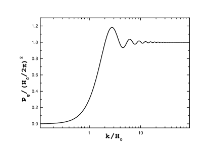
Figure 1: The power spectrum ${\cal P}_{g}$as a function of ${k\over{\cal H}_{0}}$. The x-axe is ${k\over{\cal H}_{0}}$, and the y-axe is $P_{g}/\left({{\cal H}_{0}\over 2\pi}\right)^{2}$.

For $k\ll{\cal H}_{0}$, the Hankel function can be expanded in term of a large variable, thus we have approximately

$$P_{s}\sim k^{3}$$ (27)

on large scale, which is the usual result of PBB scenario. For $k\gg{\cal H}_{0}$, the Hankel function can be expanded in term of a small variable, thus we obtain

$$P_{s}\sim k^{0}$$ (28)

on small scale, which is the result of inflation scenario. This is because the large $k$ modes are inside the horizon during the contracting phase and are not quite insensitive to the background at this stage. Thus when they cross the horizon during inflation after the transition, the nearly scale-invariant spectrum can be generated by the evolution of the background during inflationary phase. In Fig.1 we plot $P_{g}$ in (26) as a function of ${k\over{\cal H}_{0}}$. We see that for $k\sim{\cal H}_{0}$ the amplitude of the spectrum oscillates and for $k\ll{\cal H}_{0}$ it decreases rapidly and gets a cutoff. Therefore for an appropriate choice of the e-folds number of inflation, it is possible to suppress the lower multipoles of the CMB anisotropies.

Now we fit the resulting primordial spectra to the current WMAP TT and TE data. In our model the sufficient contraction makes the universe flat, so we take $\Omega_{k}=0$. We vary grid points with ranges $[0.65,0.75]$, $[0.021,0.024]$, $[0.12,0.16]$, $[0.05,0.3]$ and $[0,0.001]$ Mpc^-1 for $h$, $\Omega_{b}h^{2}$, $\Omega_{cdm}h^{2}$, $\tau$ and ${\cal H}_{0}$ respectively. At each point in the grid we use subroutines derived from those made available by the WMAP team to evaluate the likelihood with respect to the WMAP TT and TE data [3]. The overall amplitude of the primordial perturbations has been used as a continuous parameter. Tensor contribution has not been considered since $r$ can be very small. We get a minimum $\chi^{2}=1428.2$ at $h=0.73$, $\Omega_{b}h^{2}=0.024$, $\Omega_{cdm}h^{2}=0.116$, $\tau=0.2$ and ${\cal H}_{0}=2.0\times 10^{-4}$ Mpc^-1. We also run a similar code for the scale invariant spectrum for comparison and get a minimum $\chi^{2}=1429.7$ at $h=0.73$, $\Omega_{b}h^{2}=0.024$, $\Omega_{cdm}h^{2}=0.116$ and $\tau=0.2$. This means our primordial spectrum is favored at $>1.1\sigma$ than the scale invariant spectrum in our realization. ${\cal H}_{0}$ can be given in our fit with ${\cal H}_{0}\lesssim 5.0\times 10^{-4}$ Mpc^-1. However as we have set $a=1$ at the transition scale instead of today, the exact physical energy scale during the transition cannot be known due to the uncertainty in the number of e-folding and details of reheating[41, 42]. In Fig. 2 we show the resulting CMB TT multipoles and two-point temperature correlation function for the scale invariant spectrum and our spectrum with a cutoff in our parameter space. One can see that the resulting CMB TT quadrupole and the correlation function at $\theta\gtrsim 60^{\circ}$ can be much better suppressed for spectrum with a cutoff than in the scale invariant case. It is noteworthy that the uncertainty by cosmic variance plays an significant role around the smallest CMB multipoles, which is much larger than WMAP’s instrumental noise. WMAP team predicts an extremely low TT quadrupole $\delta T_{2}=123\mu K^{2}$. Meanwhile the best fit power law and running-spectral index $\Lambda$CDM model predict $\delta T_{2}=1107$ and 870 $\mu K^{2}$ respectively[1]. Our cutoff spectrum can give $\delta T_{2}$ as low as 620 $\mu K^{2}$. It is not yet compatible with WMAP quadrupole within cosmic variance limit since the lowest $\delta T_{2}$ is $620\times(1-\sqrt{2/5})\sim 228$ $\mu K^{2}$. However as claimed by Efstathiou[43] the pseudo-$C_{l}$ estimator used by the WMAP team might be non-optimal and the quadrupole is found to lie between 176 and 250 $\mu K^{2}$ and more likely to be at the upper bound of the range. Thus our model can be actually workable and future WMAP data may present a more presice check.

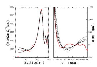
Figure 2: CMB anisotropy and two-point temperature correlation function for the scale invariant spectrum and the spectrum with a cutoff. Left: From left top to bottom, the lines stand for scale invariant spectrum, spectrum with a cutoff with ${\cal H}_{0}=2.1,3.1$ and $4.1\times 10^{-4}$ Mpc^-1. Other parameters are fixed at $h=0.73$, $\Omega_{b}h^{2}=0.023$, $\Omega_{cdm}h^{2}=0.117$ and $\tau=0.2$. Right: From right top to bottom,the lines stand for scale invariant spectrum, spectrum with a cutoff with ${\cal H}_{0}=2.1,3.1$ and $4.1\times 10^{-4}$ Mpc^-1 and the WMAP released data.

In summary, we construct a scenario in which a contracting phase is matched to an inflationary phase instantaneously. We calculate the spectrum of the scalar perturbation and find that the power spectrum on large scale is suppressed due to $\sim k^{3}$, which is the usual result of PBB scenario, and on small scale the nearly scale-invariant spectrum of inflation is recovered. Thus our scenario can provide a reasonable explanation for lower CMB anisotropies on large angular scales. Although in our proposed scenario, we neglect the physical details of the bounce, the results obtained by us reflect the generic feature of model in which the inflation phase follows the contracting phase of PBB. In our scenario, we not only obtain the suppressed lower multipoles, which is connected with the physical detail of PBB and bounce, but also avoids the initial singularity by the bounce. Furthermore, our scenario makes an attempt to improve the PBB scenario on the graceful exit problem with a period of inflation, which is worth studying further.

- [1] http://lambda.gsfc.nasa.gov/.
- [2] C. L. Bennett et al., astro-ph/0302207; E. Komatsuet al., astro-ph/0302223.
- [3] L. Verde et al., astro-ph/0302218;
- [4] D. N. Spergel et al., astro-ph/0302209; H. V. Peiris et al., astro-ph/0302225.
- [5] G. Hinshaw et al., astro-ph/0302217.
- [6] A. Kogut et al., astro-ph/0302213.
- [7] M. Fukugita and M. Kawasaki, astro-ph/0303129; Z. Haiman and G. Holder, Astrophys. J. 595, 1 (2003); R. Cen, Astrophys. J. 591, L5 (2003); A. Sokasian, N. Yoshida, T. Abel, L. Hernquist and V. Springel, astro-ph/0307451; S. Wyithe and A. Loeb, astro-ph/0302297; B. Ciardi, A. Ferrara and S. White, astro-ph/0302451; X. Chen, A. Cooray, N. Yoshida and N. Sugiyama, astro-ph/0309116; X. Chen and M. Kamionkowski, astro-ph/0310473.
- [8] P. Mukherjee and Y. Wang, astro-ph/0303211.
- [9] S. L. Bridle, A. M. Lewis, J. Weller, and G. Efstathiou, astro-ph/0302306.
- [10] U. Seljak, P. McDonald and A. Makarov, astro-ph/0302571.
- [11] V. Barger, H. Lee, and D. Marfatia, Phys.Lett.B 565, 33 (2003); W. H.Kinney, E. W.Kolb, A. Melchiorri and A. Riotto, hep-ph/0305130; S. M.Leach and A. R.Liddle, astro-ph/0306305.
- [12] B. Feng, M. Li, R.-J. Zhang, and X. Zhang, astro-ph/0302479.
- [13] J. E. Lidsey and R. Tavakol, astro-ph/0304113; M. Kawasaki, M. Yamaguchi and J. Yokoyama, Phys.Rev. D 68, 023508 (2003); Q. G. Huang and M. Li, JHEP 0306, 014 (2003); D. J. Chung, G. Shiu and M. Trodden, astro-ph/0305193; K.-I. Izawa, hep-ph/0305286; M. Bastero-Gil, K. Freese and L. Mersini-Houghton, hep-ph/0306289; M. Yamaguchi and J. Yokoyama, hep-ph/0307373; B. Wang, C. Lin and E. Abdalla, hep-th/0309175.
- [14] C. L. Bennett et al., Astrophys. J. 464, L1 (1996).
- [15] J. M. Cline, P. Crotty and J. Lesgourgues, astro-ph/0304558; G. Efstathiou, astro-ph/0306431; A. d. Oliveira-Costa, M. Tegmark, M. Zaldarriaga and A. Hamilton,astro-ph/0307282; A. Niarchou, A. H. Jaffe and L. Pogosian, astro-ph/0308461.
- [16] Y.-P. Jing and L.-Z. Fang, Phys. Rev. Lett. 73,1882 (1994); J. Yokoyama, Phys. Rev. D59, 107303 (1999).
- [17] C. R. Contaldi, M. Peloso, L. Kofman, and A. Linde, astro-ph/0303636.
- [18] S. DeDeo, R. R. Caldwell and P. J. Steinhardt, Phys.Rev.D 67, 103509 (2003) ; J. Uzan, A. Riazuelo, R. Lehoucq and J. Weeks, astro-ph/0303580 ; G. Efstathiou, Mon.Not.Roy.Astron.Soc. 343, L95 (2003); E. Gaztanaga, J. Wagg, T. Multamaki, A. Montana and D. H. Hughes, astro-ph/0304178; M. Kawasaki and F. Takahashi, hep-ph/0305319; M. Bastero-Gil et al., in Ref.[13]; A. Lasenby and C. Doran, astro-ph/0307311; S. Tsujikawa, R. Maartens and R. Brandenberger, astro-ph/0308169; T. Moroi and T. Takahashi,astro-ph/0308208; Q. Huang and M. Li, astro-ph/0308458.
- [19] B. Feng and X. Zhang, Phys.Lett.B 570, 145 (2003); X. Bi, B. Feng and X. Zhang, hep-ph/0309195.
- [20] M. H. Kesden, M. Kamionkowski and A. Cooray, astro-ph/0306597.
- [21] J. M. Diego, P. Mazzotta and J. Silk, astro-ph/0309181; O. Dore, G. P. Holder and A. Loeb, astro-ph/0309281; P. G. Castro, M. Douspis and P. G. Ferreira, astro-ph/0309320.
- [22] M. Gasperini and G. Veneziano, Astropart. Phys. 1 (1993) 317, hep-th/9211021.
- [23] G. Veneziano, hep-th/0002094; J.E. Lidsey, D. Wands and E.J. Copeland, Phys. Rept. 337 (2000) 343, hep-th/9909061. M. Gasperini and G. Veneziano, hep-th/0207130.
- [24] J. Khoury, B.A. Ovrut, P.J. Steinhardt and N. Turok, Phys. Rev. D64 (2001) 123522; J. Khoury, B.A. Ovrut, N. Seiberg, P.J. Steinhardt and N. Turok, Phys. Rev. D65 (2002) 086007; P.J. Steinhardt and N. Turok, Science 296, (2002) 1436; Phys. Rev. D65 126003 (2002).
- [25] F. Finelli and R. Brandenberger, hep-th/0112249.
- [26] Y.S. Piao and E. Zhou, hep-th/0308080, to appear in Phys. Rev. D.
- [27] N. Kanekar, V. Sahni and Shtanov, Phys. Rev. D63 (2001) 084520.
- [28] F. Finelli, hep-th/0307068.
- [29] A. Tolley and N. Turok, Phys. Rev. D66 (2002) 106005, hep-th/0204091.
- [30] I. Antoniadis, E. Gava and K.S. Narain, Nucl. Phys. B383 (1992) 93; I. Antoniadis, J. Rizos and K. Tamvakis, Nucl. Phys. B415 (1994) 497.
- [31] M. Gasperini, M. Maggiore and G. Veneziano, Nucl. Phys. B494 (1997) 315; R. Brustein and R. Madden, Phys. Rev. D57 (1998) 712.
- [32] V.F. Mukhanov, H.A. Feldman and R.H. Brandenberger, Phys. Rept. 215, 203 (1992).
- [33] J.M. Bardeen, Phys. Rev. D 22, 1882 (1980).
- [34] V.F. Mukhanov, Sov. Phys. JETP 67, 1297 (1988).
- [35] C. Cartier, R. Durrer and E.J. Copeland, Phys. Rev. D 67, 103517 (2003).
- [36] R. Durrer, hep-th/0112026; R. Durrer and F. Vernizzi, Phys. Rev. D66 (2002) 083503.
- [37] R. Brandenberger and F. Finelli, hep-th/0109004.
- [38] P. Peter and N. Pinto-Neto, hep-th/0203013; P. Peter, N. Pinto-Neto and D.A. Gonzalez, hep-th/0306005.
- [39] C. Cartier, J.C. Hwang and E.J. Copeland, Phys. Rev. D 64, 103504 (2001).
- [40] S. Tsujikawa, R. Brandenberger and F. Finelli, Phys. Rev. D 66, 083513 (2002).
- [41] D. H. Lyth and A. Riotto, Phys.Rept. 314, 1 (1999).
- [42] B. Feng, X. Gong and X. Wang, astro-ph/0301111.
- [43] G. Efstathiou, astro-ph/0310207.
- [44] U. Seljak and M. Zaldarriaga, Astrophys. J. 469, 437 (1996).
- [45] http://cmbfast.org/ .