Noncommutative solitons and instantons

Abstract

I review in this talk different approaches to the construction of vortex and instanton solutions in noncommutative field theories.

I Introduction

The development of Noncommutative Quantum Field Theories has a long story that starts with Heisenberg observation (in a letter he wrote to Peierls in the late 1930 P ) on the possibility of introducing uncertainty relations for coordinates, as a way to avoid singularities of the electron self-energy. Peierls eventually made use of these ideas in work related to the Landau level problem. Heisenberg also commented on this posibility to Pauli who, in turn, involved Oppenheimer in the discussion O . It was finally Hartland Snyder, an student of Openheimer, who published the first paper on Quantized Space Time S . Almost immediately C.N. Yang reacted to this paper publishing a letter to the Editor of the Physical Review Y where he extended Snyder treatment to the case of curved space (in particular de Sitter space). In 1948 Moyal addressed to the problem using Wigner phase-space distribution functions and he introduced what is now known as the Moyal star product, a noncommutative associative product, in order to discuss the mathematical structure of quantum mechanics M .

The contemporary success of the renormalization program shadowed these ideas for a while. But mathematicians, Connes and collaborators in particular, made important advances in the 1980, in a field today known as noncommutative geometry C . The physical applications of these ideas were mainly centered in problems related to the standard model until Connes, Douglas and Schwartz observed that noncommutative geometry arises as a possible scenario for certain low energy limits of string theory and M-theory CDS . Afterwards, Seiberg and Witten SW identified limits in which the entire string dynamics can be described in terms of noncommutative (Moyal deformed) Yang-Mills theory. Since then, 1300 papers (not including the present one) appeared in the arXiv dealing with different applications of noncommutative theories in physical problems.

Many of these recent developments, including Seiberg-Witten work, were triggered in part by the construction of noncommutative instantons NS and solitons GMS , solutions to the classical equations of motion or BPS equations of noncommutative theories. The present talk deals, precisely, with the construction of vortex solutions for the noncommutative version of the Abelian Higgs model and of instanton solutions for noncommutative Yang-Mills theory. It covers work done in collaboration with D.H. Correa, G.S. Lozano, E.F. Moreno and M.J. Rodríguez.

The plan of the talk is the following. In the next section I describe the construction of noncommutative field theories using the Moyal star product and how this can be connected, in the case of even dimensional spaces, with a Fock space formulation. The approach will allow to turn the more involved non-linear equations of motion (or BPS equations) in noncommutative space into algebraic equations which are simpler to analyze. The application of this technique to the construction of vortex solutions in the noncommutative Abelian Higgs model is presented and finally, in the last section, instanton solutions to the self-dual equation for a $U(2)$ noncommutative gauge theory are discussed.

II The connection between Moyal product of fields and operator product in Fock space

Let us call $x^{\mu}$, $\mu=1,2,...d$ the coordinates of $d$-dimensional space-time. Given $\phi(x)$ and $\chi(x)$, two ordinary functions in $R^{d}$, their Moyal product is defined as M

$$\phi(x)*\chi(x) = \left.\exp\left(\frac{i}{2}\theta_{\mu\nu}\partial^{\mu}_{x}\partial^{\nu}_{y}\right)\phi(x)\chi(y)\right|_{y=x}$$ (1)

$$= \phi(x)\chi(x)+\frac{i}{2}\theta_{\mu\nu}\partial^{\mu}\phi(x)\partial^{\nu}\chi(x)$$

$$-\frac{1}{8}\theta_{\mu\alpha}\theta_{\nu\beta}\partial_{\mu}\partial_{\alpha}\phi(x)\partial_{\nu}\partial_{\beta}\chi(x)+\ldots$$

with $\theta_{\mu\nu}$ a constant antisymmetric matrix of rank $2r\leq d$ and dimensions of $(length)^{2}$. One can easily see that (1) defines a noncommutative but associative product,

$$\phi(x)*\left(\vphantom{2^{3}}\chi(x)*\eta(x)\right)=\left(\vphantom{2^{3}}\phi(x)*\chi(x)\right)*\eta(x)$$ (2)

Under certain conditions, integration over $R^{d}$ of Moyal products has all the properties of the the trace (Tr) in matrix calculus,

$$\int dx\,\phi(x)*\chi(x)=\int dx\,\chi(x)*\phi(x)=\int dx\,\phi(x)\chi(x)$$ (3)

Indeed, identity (3) holds when derivatives of fields vanish sufficiently rapidly at infinity, since

$$\phi(x)*\chi(x) = \phi(x)\chi(x)+\frac{i}{2}\theta_{\mu\nu}\partial^{\mu}\phi(x)\partial^{\nu}\chi(x)-$$

$$\frac{1}{8}\theta_{\mu\alpha}\theta_{\nu\beta}\partial_{\mu}\partial_{\alpha}\phi(x)\partial_{\nu}\partial_{\beta}\chi(x)+\ldots$$

$$= \phi(x)\chi(x)+\partial_{\mu}\Lambda_{\mu}$$

One has also in this case cyclic property of the star product,

$$\int dx\,\phi(x)*\chi(x)*\psi(x)=\int dx\,\psi(x)*\chi(x)*\phi(x)$$ (4)

Finally, Leibnitz rule holds

$$\partial_{\mu}\left(\phi(x)*\chi(x)\right)=\partial_{\mu}\phi(x)*\chi(x)+\phi(x)*\partial_{\mu}\chi(x)$$ (5)

The $*$-commutator, denoted with $[~{},~{}]$,

$$[\phi,\chi]=\phi(x)*\chi(x)-\chi(x)*\phi(x)$$ (6)

is usually called a Moyal bracket. If one considers the case in which $\phi$ and $\chi$ correspond to space-time coordinates $x^{\mu}$ and $x^{\nu}$, one has, from eq.(1),

$$[x^{\mu},x^{\nu}]=i\theta^{\mu\nu}$$ (7)

This justifies the terminology “noncommutative space-time” although in the Moyal product approach to noncommutative field theories one takes space as the ordinary one and it is through the star multiplication of fields that noncommutativity enters into play. For example, the action for a massive self-interacting scalar field takes, in the noncommutative case, the form

$$S=\int d^{4}x\left(\partial_{\mu}\phi*\partial^{\mu}\phi-\frac{m^{2}}{2}\phi*\phi-\frac{\lambda}{4!}\phi*\phi*\phi*\phi\right)$$ (8)

Note that due to eq.(3), the quadratic part of the action coincides with the ordinary one (and hence Feynman propagators are the same for commutative and noncommutative theories). It is through interactions that differences arise.

We are interested in coupling scalars to gauge fields. Given a gauge connection $A_{\mu}$ and a gauge group element $g\in G$, the gauge connection should transform, under a gauge rotation as

$$A_{\mu}^{g}(x)=g(x)*A_{\mu}(x)*g^{-1}(x)+\frac{i}{e}g^{-1}(x)*\partial_{\mu}g(x)$$ (9)

Note that even in the $U(1)$ case, due to noncommutative multiplication, the second term in the r.h.s. has to be present in order to have a consistent definition of the curvature. Also, the expression for $g(x)$ as an exponential should be understood as

$$g(x)=\exp_{*}(i\epsilon(x))\equiv 1+i\epsilon(x)-\frac{1}{2}\epsilon(x)*\epsilon(x)+\ldots$$ (10)

Accordingly, even in the $U(1)$ case the curvature $F_{\mu\nu}$ necessarily implies a gauge field commutator,

$$F_{\mu\nu}=\partial_{\mu}A_{\nu}-\partial_{\nu}A_{\mu}-ie\left(A_{\mu}*A_{\nu}-A_{\nu}*A_{\mu}\right)$$ (11)

and then, as it happens for non Abelian gauge theories in ordinary space, the field strength $F_{\mu\nu}$ is not gauge invariant but gauge covariant,

$$F_{\mu\nu}\to g^{-1}*F_{\mu\nu}*g$$ (12)

However, due to the trace property of the integral, the Maxwell action is gauge invariant,

$$S=\frac{1}{4}\int d^{4}xF_{\mu\nu}*F^{\mu\nu}$$ (13)

As for matter fields, one can write

$$D_{\mu}^{f}\phi=\partial_{\mu}+iA_{\mu}*\phi~{}~{}~{}{\rm``fundamental"}$$

but also

$$D_{\mu}^{\bar{f}}\phi=\partial\mu-i\phi*A_{\mu}~{}~{}~{}{\rm``anti-fundamental"}$$

$${D}_{\mu}^{ad}\phi=\partial_{\mu}\phi-ie(A_{\mu}*\phi-\phi*A_{\mu})~{}~{}~{}{\rm``adjoint"}$$

Extending non-Abelian gauge theories with generators $t^{a}$ to the noncommutative case is problematic. Consider for example the case of $G=SU(N)$. In the commutative case one has

$$[A_{\mu},A_{\nu}] = A_{\mu}^{a}A_{\nu}^{b}t^{a}t^{b}-A_{\nu}^{b}A_{\mu}^{a}t^{b}t^{a}$$

(15)

$$= A_{\mu}^{a}A_{\nu}^{b}\underbrace{\left(t^{a}t^{b}-t^{b}t^{a}\right)}_{f_{abc}t_{c}}$$

so that the commutator, and a fortiori the field strength, take values, as the gauge field itself, in the Lie algebra of the gauge group. In contrast, in the noncommutative case the presence of the star product prevents to arrange the commutator as above,

$$[A_{\mu},A_{\nu}]=A_{\mu}^{a}*A_{\nu}^{b}t^{a}t^{b}-A_{\nu}^{b}*A_{\mu}^{a}t^{b}t^{a}$$

Using

$$t^{a}t^{b}=2if_{abc}t^{c}+\frac{2}{N}\delta_{ab}I+2d_{abc}t^{c}$$ (16)

we see that

$$F_{\mu\nu}=^{(1)}\!\!\!F_{\mu\nu}^{a}t^{a}+^{(2)}\!\!\!F_{\mu\nu}I$$ (17)

and hence $F_{\mu\nu}\not\in{\cal SU(N)}$. One should instead choose $U(N)$ as gauge group since, in that case, no problem of this kind arises.

III Noncommutative solitons

In order to understand the difficulties and richness one encounters when searching for noncommutative solitons, let us disregard the kinetic energy term in action (8) and just consider the scalar potential,

$$V[\phi*\phi]=\frac{1}{2}m^{2}\phi*\phi-\frac{\lambda}{4}\phi*\phi*\phi*\phi$$ (18)

The equation for its extrema is

$$m^{2}\phi-\lambda\phi*\phi*\phi=0$$ (19)

or, with the shift $\phi\to({m}/{\sqrt{\lambda}})\phi$,

$$\phi(x)*\phi(x)*\phi(x)=\phi(x)$$ (20)

To find a solution, consider a function $\phi_{0}(x)$ such that

$$\phi_{0}(x)*\phi_{0}(x)=\phi_{0}(x)$$ (21)

which evidently satisfies (20). Although simpler than (20), (21) implies, through Moyal star products, derivatives of all orders as it was the case for the original equation. Only some solutions can be found straightforwardly or with some little work. For example, in $d=2$ dimensions one finds

$$\phi_{0} = 0$$

$$\phi_{0} = 1$$

$$\phi_{0} = \frac{2}{\sqrt{\theta}}{\exp\left(-\vec{x}^{2}/\theta\right)}_{~{}~{}~{}\overrightarrow{\theta\to 0}~{}~{}~{}}\delta^{(2)}(x)$$ (22)

Already a solution like (22) shows that nontrivial regular solutions, which were excluded in the commutative space due to Derrick theorem, can be found in noncommutative space. The the reason for this is clear: the presence of the parameter $\theta$ carrying dimensions of $length^{2}$, prevents the Derrick scaling analysis leading to the negative results in ordinary space.

Finding more general solutions needs new angles of attack. A very fruitful approach was developed in GMS by exploiting an isomorphism between the algebra of functions with the noncommutative Moyal product and the algebra of operators on some Hilbert space. We shall describe this procedure below in a simple two-dimensional example (but any even dimensional space can be treated identically).

We then start with two-dimensional space with complex coordinates

$$z=\frac{1}{\sqrt{2}}(x^{1}+ix^{2})\,,\;\;\;\;\;\;\bar{z}=\frac{1}{\sqrt{2}}(x^{1}-ix^{2})$$ (23)

Changing the coordinate normalization,

$$\hat{a}=\frac{1}{\sqrt{2\theta}}(x^{1}+ix^{2})\,,\;\;\;\;\;\;\hat{a}^{\dagger}=\frac{1}{\sqrt{2\theta}}(x^{1}-ix^{2})$$ (24)

one ends with noncommutative coordinates satisfying

$$[x^{1},x^{2}]=i\theta\longrightarrow[\hat{a},\hat{a}^{\dagger}]=1$$ (25)

Then $\hat{a}$ and $\hat{a}^{\dagger}$ satisfy the algebra of annihilation and creation operators. One then considers a Fock space with a basis $|n\rangle$ provided by the eigenfunctions of the number operator $N$,

$$\hat{N}=\hat{a}^{\dagger}\hat{a}~{}~{}~{}~{}~{}~{}\hat{N}|n\rangle=n|n\rangle$$ (26)

Note that one can establish a connection between $n$ and the radial variable,

$$\hat{N}={\hat{a}}^{\dagger}\hat{a}\approx\frac{1}{2\theta}(x^{2}+y^{2})=\frac{r^{2}}{2\theta}\,,\;\;\;\theta\ \to 0$$ (27)

Configuration space at infinity then corresponds to $n\to\infty$ in Fock space. Now, it is very easy to write projectors $P_{n}$ in Fock space,

$$P_{n}=|n\rangle\langle n|\;,\;\;\;P_{n}^{2}=1$$ (28)

so that

$$P_{n}^{3}=P_{n}$$ (29)

which is nothing but the configuration space equation (20) for the minimum of the potential, but written in Fock space. So, we can say that we know a solution to (20) in operator form,

$$O_{\phi}=|n\rangle\langle n|$$ (30)

Now, how does one pass from this solution in Fock space to the corresponding solution in configuration space? The answer is to use the Weyl connection which can be summarized as follows: given a field $\phi(z,\bar{z})$ in configuration space, take its Fourier transform

$$\tilde{\phi}(k,\bar{k})=\int d^{2}z\phi(z,\bar{z})\exp\left(\frac{i}{\theta}(\bar{k}z+k\bar{z})\right)$$ (31)

with variables defined as before,

$$z=\frac{1}{\sqrt{2}}\left(x^{1}+ix^{2}\right)\;\;\;\;k=\frac{1}{\sqrt{2}}\left(k^{1}+ik^{2}\right)$$ (32)

From it, define the associated operator

$$O_{\phi}(a,a^{\dagger})=\frac{1}{4\pi^{2}\theta}\int d^{2}k\tilde{\phi}(k,\bar{k})\exp\left(-i\bar{k}a+ka^{\dagger}\right)$$ (33)

Then, one can prove that

$$\underbrace{O_{\phi}O_{\chi}}_{operator~{}product}=O_{\!\!{\underbrace{\phi*\chi}_{*\,product}}}$$ (34)

Hence, the complicated star product of fields in configuration space becomes just a simple operator product in Fock space. As an example of how this connection can be used, consider the expression for $P_{n}$ (that can be found in any textbook on second quantization)

$$|n\rangle\langle n|=:\frac{1}{m!}a^{\dagger n}\exp(-a^{\dagger}a)a^{n}:$$ (35)

(Here “$:\,:$” means normal ordering) Then, Weyl connection implies

$$:\frac{1}{m!}a^{\dagger n} \!\!\!\!\!\!\!\!\!\exp(-a^{\dagger}a)a^{n}:$$

$$= \int\frac{d^{2}k}{4\pi^{2}}\tilde{\phi}_{0}^{n}(\bar{k},k):e^{-i(k_{\bar{z}}a+k_{z}a^{\dagger})}:$$

or, anti-transforming (and using Rodrigues formula)

$$\tilde{\phi}_{0}^{n}(\bar{k},k)=2\pi\exp(-k^{2}/2)L_{n}(k^{2}/2)$$ (36)

where $L_{n}$ is the Laguerre polynomial of order $n$. Finally, Fourier transforming this expression, one can write in configuration space

$$\phi_{0}^{n}(\bar{z},z)=2(-1)^{n}\exp\left(\frac{\bar{z}z}{\theta}\right)L_{n}\left(\frac{2\bar{z}z}{\theta}\right)$$ (37)

In this way, any operator solution in Fock space can be connected with the corresponding solution in configuration space where fields are multiplied using the star product. In particular, a general solution for the minimum of the potential equation

$$\phi(\vec{x})=\phi(\vec{x})*\phi(\vec{x})*\phi(\vec{x})$$ (38)

in $d=2$ space is then,

$${\rm in~{}Fock~{}space:\hskip 28.45274pt}P_{\phi} = \sum\lambda_{n}|n\rangle\langle n|$$

$${\rm in~{}configuration~{}space:\hskip 34.14322pt}\phi = \sum\lambda_{n}\phi_{0}^{n}(\vec{x})$$

with $\lambda_{n}=0,\pm 1$ and $\phi_{0}^{n}$ given by (37).

Now, we want more than solving equations for the extrema of potentials. We then have to be able to write kinetic energy terms in Fock space. To this end, observe that

$$[a^{\dagger},a^{n}]=-na^{n-1}$$ (40)

We then see that we can identify

$$\frac{\partial f}{\partial a}=-[a^{\dagger},f(a)]$$ (41)

so that derivatives of fields $\phi$ become, in operator language,

$$\partial_{z}\phi\to-\frac{1}{\sqrt{\theta}}[a^{\dagger},O_{\phi}]\,,\;\;\;\;\;\;\partial_{\bar{z}}\phi\to{\frac{1}{\sqrt{\theta}}[a,O_{\phi}]}$$ (42)

and the Lagrangian associated to action (8) can be written in the form

$$L=\frac{1}{2}\left([a,O_{\phi}]^{2}+[a^{\dagger},O_{\phi}]^{2}\right)-\frac{m^{2}}{2}O_{\phi}^{2}+\frac{\lambda}{4}O_{\phi}^{4}$$ (43)

A last useful formula for the connection relates integration in configuration space with trace of operators in Fock space:

$${\noindent\int dxdy\phi(x,y)\;\;\;\Rightarrow}\;\;\;2\pi\theta\,{\rm Tr}\,O_{\phi}$$ (44)

From here on we shall abandon the notation $O_{\phi}$ for operators and just write $\phi$ both in configuration and Fock space.

IV Noncommutative vortices

The noncommutative version of the Abelian Higgs Lagrangian (in the fundamental representation) reads

$$L=-\frac{1}{4}F_{\mu\nu}*F^{\mu\nu}+\overline{D_{\mu}\phi}*D^{\mu}\phi-\frac{\lambda}{4}(\phi*\bar{\phi}-\eta^{2})^{2}$$ (45)

Let us briefly review how vortex solutions were found in such a model in ordinary space NO -Bogo . The energy for static, z-independent configurations is, for the commutative version of the theory,

$$E=\frac{1}{2}F_{ij}^{2}+\overline{D_{i}\phi}{D_{i}\phi}+\frac{\lambda}{4}(|\phi|^{2}-\eta^{2})^{2}$$ (46)

Here $i=1,2$ so one can consider the model in two dimensional Euclidean space with

$$D_{i}\phi=\partial_{i}-iA_{i}\phi\;,\;\;\;\phi=\phi^{1}+i\phi^{2}$$ (47)

The Nielsen-Olesen strategy to find topologically non trivial regular solutions to the equations of motion of this model in ordinary space can be summarized in the following steps going from the trivial to the vortex solution:

1. Trivial solution

   $$|\phi|={\eta}\;,\;\;\;A_{i}={0}$$ (48)

2. Topologically non-trivial but singular solution (fluxon)

   $$\phi={\eta}\exp(in\varphi)\;,\;\;\;A_{i}=n\partial_{i}\varphi$$ (49)

   with

   $$\int d^{2}x\varepsilon_{ij}F_{ij}=2\pi n$$ (50)

   but

   $$\varepsilon_{ij}F_{ij}=2\pi{n\delta^{(2)}(x)}$$ (51)

3. Regular Nielsen-Olesen vortex solution

   $$\phi={f(r)}\exp(in\varphi)\;,\;\;\;A_{i}={a(r)}\partial_{i}\varphi$$ (52)

   with boundary conditions:

   $$f(0)=a(0)=0\;,\;\;\;f(\infty)=\eta\;,a(\infty)=n$$ (53)

4. Bogomol’nyi bound

   $${\rm if~{}}\lambda=2\;,\;\;\;E\geq 2\pi n$$ (54)

   whenever the following first order “Bogomol’nyi” equations hold

   $$F_{z\bar{z}}=\eta^{2}-\bar{\phi}\phi -F_{z\bar{z}}=\eta^{2}-\bar{\phi}\phi$$

   $$D_{\bar{z}}\phi=0~{}~{}~{}~{} ~{}~{}~{}~{}D_{z}\phi=0$$

   $${\rm Selfdual~{}~{}~{}~{}} {\rm~{}~{}Antiselfdual}$$ (55)

Exact solutions of these equations can be easily constructed. Let us describe as an example the noncommutative selfdual case. One just copies the commutative strategy, starting from the “trivial” solution that we found in terms of projectors

$$\underbrace{|\phi|={\eta}}_{trivial}\hskip 5.69046pt \Rightarrow \hskip 5.69046pt\phi=\eta\sum\underbrace{f_{m}}_{0,\pm 1}|m\rangle\langle m|$$

$$\underbrace{|\phi|=\eta\exp(i\varphi)}_{singular}=\eta\frac{z}{|z|}\hskip 5.69046pt \Rightarrow \hskip 5.69046pt\phi=\eta\sum{f_{m}}|m\rangle\langle m|\hat{a}$$

$$\underbrace{|\phi|\!=\!f(r)\exp(i\varphi)}_{regular}=\!f\frac{z}{|z|}\hskip 5.69046pt \Rightarrow \hskip 5.69046pt\phi=\sum{\bar{f}_{m}}|m\rangle\langle m|\hat{a}$$

Note that in the second and third lines we have used the identification $z\to(1/\sqrt{\theta})\hat{a}$. The difference between these two formulæis that in the second the coefficients are $f_{m}=\pm 1$ while in the third one the $f_{\bar{m}}$ should be adjusted using the eqs. of motion and boundary conditions.

Of course (LABEL:numb) should be accompanied by a consistent ansatz for the gauge field,

$$\hat{A}_{z}=\sum{\bar{e}_{n}}{\hat{a}}^{\dagger}|m\rangle\langle m|$$ (57)

Differential equations (eqs. of motion or Bogomol’nyi eqs.) become algebraic recurrence relations which can be easily solved. For example, in the selfdual case one has from Bogomol’nyi equations

$$\sqrt{(n+2)}(f_{n+1}-f_{n})-e_{n}f_{n+1}=0$$

$$2\sqrt{(n+1)}e_{n-1}-e^{2}_{n-1}-2\sqrt{(n+2)}e_{n}-e^{2}_{n}$$

$$~{}\hskip 142.26378pt=-\theta\eta^{2}(f_{n}^{2}-1)$$

The appropriate condition at infinity ($|z|\to\infty$) was, in configuration space $f(|z|)\to 1$. It translates to $f_{n}\to 1$ for $n\to\infty$. Then, using $f_{0}$ as a shooting parameter, one determines $f_{1},f_{2},\ldots$ and from them one computes the magnetic field, the flux, the energy, from the expressions

$$B(r)=2\eta^{2}\sum_{n=0}^{\infty}\!(-1)^{n}\left(1-f_{n}^{2}\right)\exp\left({-\frac{r^{2}}{\theta}}\right)L_{n}(\frac{2r^{2}}{\theta})$$

$$\Phi=2\pi\theta{\rm Tr}\hat{B}=2\pi$$

$$E=2\pi\eta^{2}$$ (58)

For small $\theta$ one re-obtains the Nielsen-Olesen regular vortex solution. Exploring the whole range of $\theta\eta^{2}$, the dimensionless parameter governing noncommutativity, one finds that the vortex solution with $+1$ units of magnetic flux exists in all the $\theta$ range. As an example, we show in Figure 1 the magnetic field of a self-dual vortex with $N=1$ units of magnetic flux, for different values of $\theta$. We see that the solution approaches smoothly the commutative ($\theta=0$) limit.

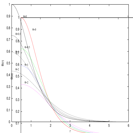
Figure 1: Magnetic field of a self-dual vortex as a function of the radial coordinate (in units of $\eta$) for different values of the anticommuting parameter $\theta$ (in units of $\eta^{2}$). The curve for $\theta=0$ coincides with that of the Nielsen-Olesen vortex in ordinary space.

In the commutative case, anti-selfdual solutions can be trivially obtained from selfdual ones by making $B\to-B$, $\phi\to\bar{\phi}$. Now, the presence of the noncommutative parameter $\theta$, breaks parity and the moduli space for positive and negative magnetic flux vortices differs drastically. One has then to carefully study this issue in all regimes, not only for $\lambda=\lambda_{BPS}$ but also for $\lambda\neq\lambda_{BPS}$, when Bogomol’nyi equations do not hold and the second order equations of motion should be analyzed. A summary of results which are obtained is (see details in (LMS1 ,LMS2 ,LMRS ):

• Positive flux

  1. There are BPS and non-BPS solutions in the whole range of $\eta^{2}\theta$. Their energy and magnetic flux are:

     For BPS solutions

     $$E_{BPS} = 2\pi\eta^{2}N\;,\;\;\;\Phi=2\pi N$$

     $$N = 1,2,\ldots$$ (59)

     For non-BPS solutions,

     $$E_{non-BPS} > 2\pi\eta^{2}N\;,\;\;\;\Phi=2\pi N$$

     $$N = 1,2,\ldots$$ (60)

  2. For $\eta^{2}\theta\to 0$ solutions become, smoothly, the known regular solutions of the commutative case.

  3. In the non-BPS case, the energy of an $N=2$ vortex compared to that of two $N=1$ vortices is a function of $\theta$.

  As in the commutative case, if one compares the energy of an $N=2$ vortex to that of two $N=1$ vortices as a function of $\lambda$ one finds that for $\lambda>\lambda_{BPS}$ $N>1$ vortices are unstable (vortices repel) while for $\lambda<\lambda_{BPS}$ they attract.

• Negative flux

  1. BPS solutions only exist in a finite range:

     $$0\leq\eta^{2}\theta\leq 1$$

     Their energy and magnetic flux are:

     $$E_{BPS} = 2\pi\eta^{2}N\;,\;\;\;\Phi=2\pi N$$

     $$N = 1,2,\ldots$$ (61)

  2. When $\eta^{2}\theta=1$ the BPS solution becomes a fluxon, a configuration which is regular only in the noncommutative case. The magnetic field of a typical fluxon solution takes the form

     $$B\sim\frac{1}{\sqrt{\theta}}{\exp(r^{2}/\theta)}_{~{}~{}~{}\overrightarrow{{\theta}\to 0}}~{}~{}\delta^{(2)}(x)~{}$$ (62)

  3. There exist non-BPS solutions in the whole range of $\theta$ but

     1. Only for $\theta<1$ they are smooth deformations of the commutative ones.

     2. For $\theta\to 1$ they tend to the fluxon BPS solution.

     3. For $\theta>1$ they coincide with the non-BPS fluxon solution.

V Noncommutative instantons

The well-honored instanton equation

$$F_{\mu\nu}=\pm\tilde{F}_{\mu\nu}$$ (63)

was studied in the noncommutative case by Nekrasov and Schwarz NS who showed that even in the $U(1)$ case one can find nontrivial instantons. The approach followed in that work was the extension of the ADHM construction, successfully applied to the systematic construction of instantons in ordinary space, to the noncommutative case. This and other approaches were discussed in i1 -in . Here we shall describe the methods developed in Cor1 ,Cor2 .

We work in four dimensional space where one can always choose

$$\theta_{12}=-\theta_{21}=\theta_{1}$$

$$\theta_{34}=-\theta_{43}=\theta_{2}$$

$${\rm all~{}other~{}}\theta^{\prime}s=0$$

We define dual tensors as

$$\tilde{F}_{\mu\nu}=\frac{1}{2}\sqrt{g}\,\varepsilon_{\mu\nu\alpha\beta}F^{\alpha\beta}$$ (64)

with $g$ the determinant of the metric.

In order to work in Fock space as we did in the case of noncommutative vortices, we now need two pairs of creation annihilation operators,

$$x^{1}\pm ix^{2}~{}~{}~{} {\Rightarrow} ~{}~{}~{}{\hat{a}}_{1},\;\;{\hat{a}}^{\;\dagger}_{1}$$

$$x^{3}\pm ix^{4}~{}~{}~{} {\Rightarrow} ~{}~{}~{}{\hat{a}}_{2},\;\;{\hat{a}}^{\;\dagger}_{2}$$

and the Fock vacuum will be denoted as $|00\rangle$. Concerning projectors the connection with configuration space takes the form

$$|n_{1}n_{2}\rangle\langle n_{1}n_{2}| {\Rightarrow} \exp\left(-r_{1}^{2}/\theta_{1}-r_{2}^{2}/\theta_{2}\right)L_{n_{1}}\left(2r_{1}^{2}/\theta_{1}\right)\times$$ (65)

$$L_{n_{2}}\left(2r_{2}^{2}/\theta_{2}\right)$$

Finally, note that the gauge group $SU(2)$ (for which ordinary instantons were originally constructed) should be replaced by $U(2)$ so that

$$A_{\mu}=A_{\mu}^{a}\frac{\sigma^{a}}{2}+A_{\mu}^{4}\frac{I}{2}$$ (66)

Let us now analyze how the different ansatz leading to ordinary instantons can be adapted to the noncommutative case.

1- (Commutative)’t Hooft multi-instanton ansatz (1976)

$$A_{\mu}(x)=\tilde{\Sigma}_{\mu\nu}j_{\nu}$$

$$\tilde{\Sigma}_{\mu\nu}=\frac{1}{2}\bar{\eta}_{a\mu\nu}\sigma^{a}\;,\;\;\;\bar{\eta}_{a\mu\nu}=\left\{\begin{array}[]{l}~{}\varepsilon_{a\mu\nu}\;,\;\;\;\mu,\nu\neq 4\\ ~{}~{}\delta_{a\mu}\;,\;\;\;\nu=4\\ -\delta_{a\nu}\;,\;\;\;\mu=4\end{array}\right.$$ (70)

$$j_{\nu}=\phi^{-1}\partial_{\nu}\phi$$

Here $\sigma^{a}$ are the Pauli matrices (’t Hooft ansatz corresponds to an $SU(2)$ gauge theory). With this ansatz, the instanton selfdual equation becomes

$$F_{\mu\nu}=\tilde{F}_{\mu\nu}~{}~{}~{}\Rightarrow~{}~{}~{}\frac{1}{\phi}\nabla\phi=0$$ (71)

with

$$\phi=1+\sum_{i=1}^{N}\frac{\lambda_{i}^{2}}{(x-c_{i})^{2}}\;,\;\;\;\nabla\phi=\sum_{i=1}^{N}\delta^{(4)}(x-c_{i})$$ (72)

The solution corresponds to a regular instanton of topological charge $Q=N$.

2- Noncommutative version of ’t Hooft ansatz

The natural way of extending ’t Hooft ansatz is to proceed with the changes

$$j_{\nu}=\phi^{-1}\partial_{\nu}\phi~{}~{}~{}\Rightarrow~{}~{}~{}j_{\nu}=\phi^{-1}*\partial_{\nu}\phi+\partial_{\nu}\phi*\phi^{-1}$$

$${A_{\mu}^{a}\frac{\sigma^{a}}{2}=\bar{\Sigma}_{\mu\nu}j_{\nu}}~{}~{}~{}\Rightarrow~{}~{}~{}A_{\mu}^{a}\frac{\sigma^{a}}{2}=\bar{\Sigma}_{\mu\nu}j_{\nu}$$ (73)

$$A_{\mu}^{4}=-i\left(\phi^{-1}*\partial_{\nu}\phi-\partial_{\nu}\phi*\phi^{-1}\right)$$ (74)

With this we see that the Poisson equation (72) for ordinary instantons changes according to

$$\frac{1}{\phi}\nabla\phi=0~{}~{}~{}\Rightarrow~{}~{}~{}\phi^{-1}*\nabla\phi*\phi^{-1}=0$$

$$\nabla\phi=\delta^{(4)}(x)\Rightarrow~{}~{}~{}\nabla\phi=\frac{\lambda^{2}}{\theta_{1}\theta_{2}}|00\rangle\langle 00|$$ (75)

One then gets, for the field strengths,

$$F=\tilde{F}+|00\rangle\langle 00|$$ (76)

We see that the self-dual equation is not exactly satisfied: the $|00\rangle\langle 00|$ term, the analogous to the delta function in the ordinary case, is not cancelled as it happened with the delta function source for the Poisson equation (71) in the commutative case.

3- Noncommutative BPST ($Q=1$) ansatz (1975)

The pioneering Belavin, Polyakov, Schwarz and Tyupkin ansatz BPST leading to the first $Q=1$ instanton solution was similar to the ’t Hooft ansatz except that $\Sigma_{\mu\nu}$ was used instead of its dual $\tilde{\Sigma}_{\mu\nu}$. Its noncommutative extension can be envisaged as

$${A_{\mu}^{a}\frac{\sigma^{a}}{2}=\Sigma_{\mu\nu}j_{\nu}}~{}~{}~{}\Rightarrow~{}~{}~{}A_{\mu}^{a}\frac{\sigma^{a}}{2}=\Sigma_{\mu\nu}j_{\nu}$$ (77)

where $j_{\nu}$ is defined as in the previous ansatz. Concerning $A_{\mu}^{4}$, the consistent ansatz changes due to the use of $\Sigma_{\mu\nu}$ instead of its dual as in the ’t Hooft ansatz. One needs now, instead of (74),

$$A_{\mu}^{4}=i\left(\phi^{-1}*\partial_{\nu}\phi+3\partial_{\nu}\phi*\phi^{-1}\right)$$ (78)

With this, one finally has

$$F_{\mu\nu}=\tilde{F}_{\mu\nu}\;,\;\;\;Q=S=1$$ (79)

but, due to the necessity of the consistent ansatz for the $A_{\mu}^{4}$ component, one can see that

$$F_{\mu\nu}\neq F_{\mu\nu}^{\dagger}$$ (80)

and hence the price one is paying in order to have a selfdual field strength is its non-hermiticity. Note however that the action and the topological charge are real.

4- (Commutative) Witten ansatz (1977)

The clue in this ansatz Witi is to reduce the four dimensional problem to a two dimensional one through an axially symmetric N-instanton ansatz. That is, one passes from 4 dimensional Euclidan space to 2 dimensional space, ($x^{1},x^{2},x^{3},x^{4}\to r,t$) but this last with a nontrivial metric $g^{ij}=r^{2}\delta^{ij},~{}i,j=1,2$.

The axially symmetric ansatz for the gauge field components is

$$\vec{A}_{r} = A_{r}(r,t)\vec{\Omega}(\vartheta,\varphi)$$

$$\vec{A}_{t} = A_{t}(r,t)\vec{\Omega}(\vartheta,\varphi)$$

$$\vec{A}_{\vartheta} = \phi_{1}(r,t)\partial_{\vartheta}\vec{\Omega}(\vartheta,\varphi)$$

$$+ \left(1+\phi_{2}(r,t)\right)\vec{\Omega}(\vartheta,\varphi)\wedge\partial_{\vartheta}\vec{\Omega}(\vartheta,\varphi)$$

$$\vec{A}_{\varphi} = \phi_{1}(r,t)\partial_{\varphi}\vec{\Omega}(\vartheta,\varphi)$$ (81)

$$+ \left(1+\phi_{2}(r,t)\right)\vec{\Omega}(\vartheta,\varphi)\wedge\partial_{\varphi}\vec{\Omega}(\vartheta,\varphi)$$

with

$$\vec{\Omega}(\vartheta,\varphi)=\left(\begin{array}[]{c}\sin\vartheta\cos\varphi\\ \sin\vartheta\sin\varphi\\ \cos\vartheta\end{array}\right)$$ (82)

With this ansatz, the selfduality instanton equation (63) becomes a pair of BPS equations for vortices in curved space

$$F_{\mu\nu}=\tilde{F}_{\mu\nu} \to \left\{\begin{array}[]{l}\frac{1}{\sqrt{g}}F_{z\bar{z}}=|\phi|^{2}-1\\ D_{z}\phi=0\end{array}\right.$$ (85)

where $\phi=\phi_{1}+i\phi_{2}$ and $z=t+ir$. Solving these BPS vortex equations then reduces to finding the solution of a Liouville equation. In this way an exact axially symmetry N-instanton solution was constructed in Witi for the (commutative)$SU(2)$ theory.

4-Noncommutative version of Witten ansatz

To proceed, one needs a noncommutative setting for curved 2-dimensional space, where $\theta$ can in principle depend on $x$,

$$[x^{i},x^{j}]=\theta^{ij}(x)$$ (86)

Now, handling such a commutator is not trivial since not all functions $\theta_{ij}(x)$ will guarantee a noncommutative but associative product.

One can see, however, that associativity can be achieved whenever

$$\nabla_{i}\theta^{ij}=0$$ (87)

In the present 2 dimensional case, these equations have as solution

$$\theta_{ij}=\theta_{0}\frac{\varepsilon_{ij}}{\sqrt{g}}$$ (88)

with $\theta_{0}$ a constant. Then, given the metric in which the instanton problem with axial symmetry reduces to a vortex problem we see that an associative noncommutative product should take the form

$$[r,t]=r^{2}\theta_{0}\;;\;\;\;all~{}other~{}[.,.]=0$$ (89)

with now $r$ and $t$ defining the two dimensional variables in curved space. A further simplification occurs after the observation that

$$r*t-t*r=r^{2}\theta_{0}~{}~{}~{}\Rightarrow~{}~{}~{}t*\frac{1}{r}-\frac{1}{r}*t=\theta_{0}$$ (90)

Then, calling $y^{1}=t$ and $y^{2}=1/r$ we have instead of (89) the usual flat space Moyal product and the Bogomol’nyi equations take the form

$$\left(1-\frac{1}{2}(z+\bar{z})^{2}\right)D_{z}\phi = \left(1+\frac{1}{2}(z+\bar{z})^{2}\right)D_{\bar{z}}\phi$$ (91)

$$iF_{z\bar{z}} = 1-\frac{1}{2}[\phi,\bar{\phi}]_{+}$$ (92)

$$iF_{z\bar{z}} = -\frac{1}{2}[\phi,\bar{\phi}]$$ (93)

with $z=y^{1}+iy^{2}$. We can at this point apply the Fock space method detailed above for constructing vortex solutions. In the present case, consistency of eqs.(91)-(93) imply

$$\bar{\phi}\phi=1$$ (94)

and hence the only kind of nontrivial ansatz should lead, in Fock space, to a scalar field of the form

$$\phi=\sum_{n=0}|n+q\rangle\langle n|$$ (95)

where $q$ is some fixed positive integer. With this, it is easy now to construct a class of solutions analogous to those previously found for vortices in flat space. It takes the form

$$\phi = \sum_{n=0}|n+q\rangle\langle n|$$

$$A_{z} = -\frac{i}{\sqrt{\theta_{0}}}\sum_{n=0}^{q-1}\left(\sqrt{n+1}\right)|n+1\rangle\langle n|+$$

$$+ \frac{i}{\sqrt{\theta_{0}}}\sum_{n=q}\left(\sqrt{n+1-q}-\sqrt{n+1}\right)|n+1\rangle\langle n|$$

One can trivially verify that configurations (LABEL:solucion) satisfy eqs.(91)-(93) provided $\theta_{0}=2$. In particular, both the l.h.s. and r.h.s of eq.(91) vanish separately. The field strength associated to our solution reads, in Fock space,

$$iF_{z\bar{z}}=-\frac{1}{2}\left(|0\rangle\langle 0|+\ldots+|q-1\rangle\langle q-1|\right)\equiv B$$ (97)

or, in the original spherical coordinates

$$\vec{F}_{tu} = B(r)\vec{\Omega}$$

$$\vec{F}_{\vartheta\varphi} = B(r)\sin\vartheta\,\vec{\Omega}$$

$$F_{tu}^{4} = B(r)$$

$$F_{\vartheta\varphi}^{4} = B(r)\sin\vartheta$$ (98)

As before, starting from (97) for $B$ in Fock space, we can obtain the explicit form of $B(r)$ in configuration space in terms of Laguerre polynomials, using eq.(65). Concerning the topological charge, it is then given by

$$Q = \frac{1}{32\pi^{2}}{\rm tr}\int d^{4}x{\varepsilon}^{\mu\nu\alpha\beta}F_{\mu\nu}F_{\alpha\beta}$$ (99)

$$= \frac{1}{\pi}\int_{-\infty}^{0}du\int_{-\infty}^{\infty}dtB^{2}=2{\rm Tr}B^{2}=\frac{q}{2}$$

We thus see that $Q$ can be in principle integer or semi-integer, and this for an ansatz which is formally the same as that proposed in Witi for ordinary space and which yielded in that case to an integer. The origin of this difference between the commutative and the noncommutative cases can be traced back to the fact that in the former case, boundary conditions were imposed on the half-plane and forced the solution to have an associated integer number. In fact, if one plots Witten’s vortex solution in ordinary space in the whole $(r,t)$ plane, the magnetic flux has two peaks and the corresponding vortex number is even. Then, in order to parallel this treatment in the noncommutative case one should impose the condition $q=2N$.

Acknowledgements: I would like to thank the organizers of the XXIV Encontro Nacional de Física de Partículas e Campos at Caxambu for inviting me to deliver a talk at such an impressive meeting and for their warm hospitality. This work is partially supported by UNLP, CICBA, ANPCYT, Argentina.

References

- (1) See Wolfgang Pauli, Scientific Correspondence, Vol II, p.15, Ed. Karl von Meyenn, Springer-Verlag, 1985.
- (2) See Wolfgang Pauli, Scientific Correspondence, Vol III, p.380, Ed. Karl von Meyenn, Springer-Verlag, 1993.
- (3) H.S. Snyder, Quantized Space-Time, Phys. Rev. 71 (1947) 38.
- (4) C. N. Yang, On Quantized Space-Time, Phys. Rev. 72 (1947) 874.
- (5) J. E. Moyal, Quantum Mechanics As A Statistical Theory, Proc. Cambridge Phil. Soc. 45 (1949) 99.
- (6) A. Connes, Noncommutative geometry, Academic Press, New York, 1994.
- (7) A. Connes, M. R. Douglas and A. Schwarz, Noncommutative geometry and matrix theory: Compactification on tori, JHEP 9802 (1998) 003.
- (8) N. Seiberg and E. Witten, String theory and noncommutative geometry, JHEP 9909 (1999) 032.
- (9) N. Nekrasov and A. Schwarz, Instantons on noncommutative R**4 and (2,0) superconformal six dimensional theory, Commun. Math. Phys. 198 (1998) 689
- (10) R. Gopakumar, S. Minwalla and A. Strominger, Noncommutative solitons, JHEP 0005 (2000) 020
- (11) H. B. Nielsen and P. Olesen, Vortex-Line Models For Dual Strings, Nucl. Phys. B 61 (1973) 45.
- (12) H. J. de Vega and F. A. Schaposnik, A Classical Vortex Solution Of The Abelian Higgs Model, Phys. Rev. D 14 (1976) 1100.
- (13) E. B. Bogomolny, Stability Of Classical Solutions, Sov. J. Nucl. Phys. 24 (1976) 449 [Yad. Fiz. 24 (1976) 861].
- (14) D. P. Jatkar, G. Mandal and S. R. Wadia, Nielsen-Olesen vortices in noncommutative Abelian Higgs model, JHEP 0009 (2000) 018
- (15) A. P. Polychronakos, Flux tube solutions in noncommutative gauge theories, Phys. Lett. B 495 (2000) 407.
- (16) J. A. Harvey, P. Kraus and F. Larsen, Exact noncommutative solitons, JHEP 0012 (2000) 024
- (17) D. Bak, Exact multi-vortex solutions in noncommutative Abelian-Higgs theory, Phys. Lett. B 495 (2000) 251
- (18) G. S. Lozano, E. F. Moreno and F. A. Schaposnik, Nielsen-Olesen vortices in noncommutative space, Phys. Lett. B 504 (2001) 117.
- (19) G. S. Lozano, E. F. Moreno and F. A. Schaposnik, Self-dual Chern-Simons solitons in noncommutative space JHEP 0102 (2001) 036.
- (20) A. Khare and M. B. Paranjape, Solitons in 2+1 dimensional non-commutative Maxwell Chern-Simons Higgs theories, JHEP 0104 (2001) 002.
- (21) D. Bak, K. M. Lee and J. H. Park, Noncommutative vortex solitons, Phys. Rev. D 63 (2001) 125010.
- (22) G. S. Lozano, E. F. Moreno, M. J. Rodriguez and F. A. Schaposnik, Non BPS noncommutative vortices, arXiv:hep-th/0309121.
- (23) K. Hashimoto and H. Ooguri, Seiberg-Witten transforms of noncommutative solitons, Phys. Rev. D 64 (2001) 106005
- (24) O. Lechtenfeld and A. D. Popov, Noncommutative multi-solitons in 2+1 dimensions, JHEP 0111 (2001) 040
- (25) R. Gopakumar, M. Headrick and M. Spradlin, On noncommutative multi-solitons, Commun. Math. Phys. 233 (2003) 355
- (26) F. Franco-Sollova and T. A. Ivanova, On noncommutative merons and instantons, J. Phys. A 36 (2003) 4207
- (27) D. Tong, The moduli space of noncommutative vortices, J. Math. Phys. 44 (2003) 3509
- (28) A. Hanany and D. Tong, Vortices, instantons and branes JHEP 0307 (2003) 037
- (29) K. Furuuchi, Instantons on noncommutative R**4 and projection operators, Prog. Theor. Phys. 103 (2000) 1043.
- (30) A. Schwarz, Noncommutative instantons: A new approach Commun. Math. Phys. 221 (2001) 433.
- (31) D. H. Correa, G. S. Lozano, E. F. Moreno and F. A. Schaposnik, Comments on the U(2) noncommutative instanton, Phys. Lett. B 515 (2001) 206
- (32) S. Parvizi, Non-commutative instantons and the information metric Mod. Phys. Lett. A 17 (2002) 341.
- (33) K. Y. Kim, B. H. Lee and H. S. Yang, Noncommutative instantons on R**2(NC) x R**2(C) Phys. Lett. B 523 (2001) 357.
- (34) O. Lechtenfeld and A. D. Popov, Noncommutative ’t Hooft instantons, JHEP 0203 (2002) 040.
- (35) D. H. Correa, E. F. Moreno and F. A. Schaposnik, Some noncommutative multi-instantons from vortices in curved space, Phys. Lett. B 543 (2002) 235
- (36) F. Franco-Sollova and T. A. Ivanova, On noncommutative merons and instantons J. Phys. A 36 (2003) 4207.
- (37) Z. Horvath, O. Lechtenfeld and M. Wolf, Noncommutative instantons via dressing and splitting approaches, JHEP 0212 (2002) 060.
- (38) T. A. Ivanova and O. Lechtenfeld, Noncommutative multi-instantons on R**2n x S**2, Phys. Lett. B 567 (2003) 107.
- (39) A. A. Belavin, A. M. Polyakov, A. S. Shvarts and Y. S. Tyupkin, Pseudoparticle Solutions Of The Yang-Mills Equations, Phys. Lett. B 59 (1975) 85.
- (40) E. Witten, Some Exact Multipseudoparticle Solutions Of Classical Yang-Mills Theory, Phys. Rev. Lett. 38 (1977) 121.