UAB-FT-522

Scherk-Schwarz Supersymmetry Breaking
with Radion Stabilization

G. v. Gersdorff , M. Quirós , A. Riotto 

^1, 2 Theoretical Physics Group, IFAE
E-08193 Bellaterra (Barcelona), Spain

² Institució Catalana de Recerca i Estudis Avançats (ICREA)

³ Department of Physics and INFN,
Sezione di Padova, via Marzolo 8, I-35131 Padova, Italy

Abstract

We study the issue of radion stabilization within five-dimensional supersymmetric theories compactified on the orbifold $S^{1}/\mathbb{Z}_{2}$. We break supersymmetry by the Scherk-Schwarz mechanism and explain its implementation in the off-shell formulation of five dimensional supergravity in terms of the tensor and linear compensator multiplets. We show that radion stabilization may be achieved by radiative corrections in the presence of five-dimensional fields which are quasi-localized on the boundaries through the presence of $\mathbb{Z}_{2}$ odd mass terms. For the mechanism to work the number of quasi-localized fields should be greater than $2+N_{V}-N_{h}$ where $N_{V}$ and $N_{h}$ are the number of massless gauge- and hypermultiplets in the bulk. The radion is stabilized in a metastable Minkowski vacuum with a lifetime much larger than cosmological time-scales. The radion mass is in the meV range making it interesting for present and future measurements of deviations from the gravitational inverse-square law in the submillimeter range.

1 Introduction

Supersymmetry plays a crucial role in constructing consistent high-energy physics theories and an important issue is to explain how supersymmetry is spontaneously broken in the low-energy world. Recent ideas on extra dimensions and the speculation that our visible universe coincides with a four-dimensional (4D) brane living in the bulk of the extra dimensions – the so-called brane-world scenarios – have given rise to new appealing possibilities regarding how to realize supersymmetry breaking [1, 2, 3, 4, 5, 6, 7, 8, 9, 10]. In particular, non-trivial boundary conditions imposed on fields can affect the supersymmetries of the theory. This mechanism was proposed long ago by Scherk and Schwarz (SS) [11] and can be interpreted as spontaneous breaking of local supersymmetry through a Wilson line in the supergravity completion of the theory [12].

In this paper we want to address the issue of stabilization of the radius of the extra dimension within five-dimensional (5D) supersymmetric theories compactified on the orbifold $S^{1}/\mathbb{Z}_{2}$ where supersymmetry is broken by the Scherk-Schwarz mechanism. These models generically exhibit a structure with a vanishing (flat) potential for the radion, the field whose vacuum expectation value (VEV) determines the size $R$ of the extra dimension. Our goal is to show that the size of the fifth dimension can be fixed in the presence of five-dimensional fields which are quasi-localized on the boundaries of the 5D bulk.

The wave functions of zero-modes of matter fields can be localized towards the boundaries by adding a bulk mass-term with a non-trivial profile in the fifth dimension [13]. In particular we will be interested in 5D hypermultiplets with common odd-parity bulk masses $M$. Such mass terms can also appear from localized Fayet-Iliopoulos (FI) terms corresponding to a $U(1)$ gauge group under which hypermultiplets are charged. These FI terms, even when absent at tree-level, can be generated radiatively [14, 15]. However the existence of supersymmetric odd mass terms for hypermultiplets is more general and can even happen irrespective of possible $U(1)$ factors in the gauge group. Since we are interested in an extra dimension of size $\sim$ TeV^-1, we will take $M$ to be in the TeV range. The potential of the radion, the Casimir energy, gets a contribution from the quasi-localized fields and the radion is stabilized with a mass in the meV range. In order to ensure vanishing 4D cosmological constant we introduce bulk cosmological constant and brane tensions as counterterms, which renders the Minkowski vacuum metastable with a stable AdS vacuum. We show that the Minkowski vacuum turns out to be stable on cosmological times.

The paper is organized as follows. In section 2 we comment on the Scherk-Schwarz supersymmetry breaking mechanism and its implementation in off-shell 5D supergravity. Section 3 is devoted to the issue of radion stabilization and the computation of the lifetime of the metastable Minkowski vacuum. Finally, we present our conclusions and discussion of open problems in section 4.

2 Scherk-Schwarz supersymmetry breaking

Scherk-Schwarz (SS) supersymmetry breaking [11] of a 5D supersymmetric theory compactified on $S^{1}/\mathbb{Z}_{2}$ can be interpreted as spontaneous breaking of 5D local supersymmetry [12]. It requires the off-shell version of 5D supergravity where an auxiliary field $\vec{V}_{M}$ gauges the $SU(2)_{R}$ symmetry. This theory has been worked out in Refs. [16, 17] where it was shown that on top of the minimal irreducible $40_{B}+40_{F}$ supergravity multiplet containing the graviton ($e_{M}^{A}$), gravitino ($\psi_{M}$), graviphoton ($A_{M}$) and auxiliary fields, an aditional $8_{B}+8_{F}$ supermultiplet is needed which plays the role of a compensator multiplet and is purely auxiliary. The most convenient choice for the compensator multiplet in order to discuss SS supersymmetry breaking is the so-called tensor multiplet consisting of an $SU(2)_{R}$ triplet $\vec{Y}$, a fermionic $SU(2)_{R}$ doublet $\rho$, a three-form tensor field $B_{MNP}$ and a real scalar $N$. The minimal multiplet contains a real auxiliary scalar $C$ which enters in the action only through the term

$$C\left(1-(\vec{Y}\vec{Y})^{\frac{1}{2}}\right).$$ (2.1)

The field $\vec{Y}$ is then constrained to obey $\vec{Y}\vec{Y}=1$ which breaks $SU(2)_{R}$ spontaneously down to $U(1)_{R}$. A convenient gauge fixing is provided by

$$\vec{Y}=\left(0,1,0\right),$$ (2.2)

such that the surviving $U(1)_{R}$ is generated by $\sigma_{2}$. After this gauge fixing the gravitino kinetic term is only covariant with respect to $U(1)_{R}$ according to 

$$\mathcal{D}_{M}=D_{M}-i\frac{\sigma_{2}}{2}V_{M},$$ (2.3)

where $D_{M}$ is the usual covariant derivative containg spin- and other possible gauge connections. In the background $V_{5}$ the gravitino receives a mass and supersymmetry is spontaneously broken. The same holds true for other $SU(2)_{R}$ non-singlets such as hyperscalars and gauginos which are doublets and possible matter in tensor-multiplets which contain bosonic $SU(2)_{R}$-triplets. SS supersymmetry breaking has also been studied in the context of gauged (AdS-) supergravity [18, 19]. In the off-shell version we are using one can gauge the remaining $U(1)_{R}$-symmetry straightforwardly [17]. The equations of motion then yield that $V_{M}$ is proportional to $gA_{M}$ where $g$ is the AdS gauge coupling. A non-zero VEV for the fifth component of the graviphoton $A_{5}$ thus induces a VEV for the auxiliary field $V_{5}$. Our (tree-level) supergravity action corresponds to ungauged supergravity with $g=0$.

Let us see under which circumstances the VEV of $V_{5}$ is either undetermined at tree-level or fixed by an explicit source. The former case is realized by integrating out the three-form-field of the compensator tensor multiplet [20] (section 2.1), while supersymmetry-breaking can be realized at tree level by switching to a dual theory in terms of the so-called linear multiplet [21] (section 2.2). Both theories are equivalent locally and only differ by their global properties although we will also show that there exists a linear-multiplet formulation which is globally equivalent to the tensor one.

2.1 Tensor multiplet formalism

It turns out that after integrating out all auxiliary fields except $V_{M}$ and $B_{MNP}$, the Lagrangian containing the latter fields is

$$\mathcal{L}=-V_{M}W^{M}+W^{M}W_{M},$$ (2.4)

where the field strength of the three-form tensor field is given by

$$W^{M}=\frac{1}{12}\epsilon^{MNPQR}\partial_{N}B_{PQR}-J^{M}$$ (2.5)

and the gravitino current $J^{M}$ is defined to be

$$J^{M}=-\frac{1}{4}\overline{\psi}_{P}\gamma^{PMQ}\sigma^{2}\psi_{Q}.$$ (2.6)

Note that Eq. (2.4) is covariant with respect to $U(1)_{R}$ transformations once the full Lagrangian is considered, since the first term makes part of the covariant gravitino derivative. In order to perform the integral over $B$ properly  we linearize the $B$-dependent terms by introducing an auxiliary field $X_{M}$

$$\mathcal{L}=-V_{M}W^{M}+W^{M}X_{M}-\frac{1}{4}X_{M}X^{M}.$$ (2.7)

Varying with respect to $B$ we find the equation

$$C_{MN}\equiv 2\partial_{[M}(V-X)_{N]}=0.$$ (2.8)

We implement this condition by a functional delta in the path-integral

$$\delta[C_{MN}]=\lim_{\xi\to 0}\exp\left(-i\frac{1}{2\xi}C_{MN}C^{MN}\right)$$ (2.9)

where we have omitted a $\xi$-dependent but irrelevant normalization factor . We thus get the Lagrangian

$$\mathcal{L}=-\frac{1}{2\xi}C_{MN}C^{MN}+(V_{M}-X_{M})J^{M}-\frac{1}{4}X_{M}X^{M}$$ (2.10)

where the theory is understood in the limit $\xi\to 0$. We now make a shift of variables in the path integral $V_{M}\to V_{M}+X_{M}$ and finally integrate over $X_{M}$ to obtain:

$$-\frac{1}{2\xi}V_{MN}V^{MN}+V_{M}J^{M}$$ (2.11)

where $V_{MN}=2\partial_{[M}V_{N]}$ is the field strength of $V$. Eq. (2.11) fixes $V_{M}$ to be a closed form in the limit $\xi\to 0$ and thus it can have a non-zero flux:

$$\frac{1}{2\pi}\oint dx^{5}\langle V_{5}\rangle\equiv 2\omega.$$ (2.12)

This nontrivial flux can be removed by a nonperiodic gauge-transformation thereby transmuting the explicit mass terms for $SU(2)_{R}$ non-singlets into Scherk-Schwarz boundary conditions for those fields.

In short in the tensor multiplet formalism, after integrating out all auxiliary fields at the tree-level, one gets that $V$ is a closed but not necessarily an exact form. In spaces which allow for a non-trivial cohomology this means that $V$ can have a non-vanishing but (at tree-level) undetermined Wilson flux as in Eq. (2.12). Fixing $\langle V_{5}\rangle$ (i.e. the Wilson flux) should then be done by higher-loop corrections. It is important to realize that this procedure does not violate non-renormalization theorems: these imply that if there is a classical supersymmetric minimum for an auxiliary field its energy remains zero after including quantum corrections. Furthermore any other dynamically generated minimum should have negative energy and would be outside the validity regime of perturbation theory. One concludes that a classical supersymmetric minimum is not renormalized. The fundamental difference in our case is that there is no such classical minimum and the tree-level potential for $V_{5}$ is exactly flat. We therefore conclude that our perturbative analysis should be valid .

To conclude we will comment on the Lagrangian (2.11) that is singular in the limit $\xi\to 0$. The general strategy is then to first compute physical observables as functions of $\xi$ and then take the $\xi\to 0$ limit. In particular any observables obtained by exchanging $V_{M}$ as internal lines will vanish in that limit. Moreover quantities where $V_{M}$ are external lines, as the effective potential $V_{\rm eff}(V_{5})$, will be insensitive to that limit.

2.2 Linear multiplet formalism

In this section we will present a formulation which uses the so-called linear multiplet as the compensator for the $SU(2)_{R}$ symmetry. It consists of the fields $(\vec{Y},\rho,N,W_{A})$ where $W$ obeys the constraint $\partial_{M}(W^{M}+J^{M})=0$ or in the language of differential forms

$$d\!*\!(W+J)=0$$ (2.13)

in order to ensure closure of the supersymmetry algebra. Of course the tensor multiplet is a special case of the linear multiplet where the constraint is explicitely solved by a three-form potential for $W$. The difference of the tensor multiplet and the linear multiplet lies in the additional global constraint on the former

$$\intop\!*(W+J)=0.$$ (2.14)

where the integral goes over any four-cycle. This constraint must be implemented if we insist on a completely equivalent description of the tensor multiplet in terms of the linear multiplet. A caveat of the linear multiplet formalism is that the full gauge invariant off-shell action cannot be written in terms of the linear multiplet (see the analogous result in 4D $N=2$ supergravity [22]). However, after gauge-fixing the action for the tensor-multiplet only depends on $dB$ and consequently one can consider the field strength as the independent variable and ensure constraints (2.13) and (2.14) by introducing a Lagrange multiplier.

Before doing so let us study an intriguing possible interaction of the linear multiplet. Consider a generic vector field $E_{M}$ with vanishing field strength $dE=0$. Then we can define a Maxwell-multiplet

$$\mathbb{E}\equiv(E_{M},M=0,\Omega=0,\vec{X}=0).$$ (2.15)

where all other components except $E_{M}$ (i.e. the scalar $M$, the gaugino $\Omega$ and the auxiliary triplet $\vec{X}$) are set to zero. This configuration is left invariant under local supersymmetry transformations with parameter $\epsilon(x^{M})$, since $\delta_{\epsilon}\mathbb{E}$ only depends on $E_{M}$ through its field strength $dE$. This multiplet has no physical degrees of freedom, however on non-simply connected spaces it can have a flux $\int E_{M}dx^{M}$ which might have some physical impact. Let us therefore refer to $\mathbb{E}$ as the flux multiplet. Under the $\mathbb{Z}_{2}$ compactification with $E_{5}$ even, the flux-multiplet reduces to the constant multiplet $(\int E_{5}dx^{5},0,\dots)$ which is known to be locally supersymmetric . Using the locally supersymmetric coupling of a tensor- to a Maxwell-multiplet [17] we find the Lagrangian

$$\left(W^{M}+J^{M}\right)E_{M}-\frac{1}{2\xi}\left(E_{MN}\right)^{2}$$ (2.16)

where we already performed the gauge-fixing (2.2). The last term is again the functional delta already encountered in Eq. (2.9). It ensures the constraint $dE=0$ in the limit $\xi\to 0$. Let us stress that this term is needed to ensure supersymmetry since for $dE\neq 0$ the multiplet Eq. (2.15) is not supersymmetric. However we expect a violation of supersymmetry to $\mathcal{O}(\xi)$.

We will use the interaction Eq. (2.16) to enforce the local and global constraints (2.13) and (2.14). Indeed, varying Eq. (2.16) with respect to $E$ we find (in the language of differential forms)

$$*(W+J)=\frac{1}{\xi}d\!*\!dE.$$ (2.17)

We see that now the local and global constraints on $W$ are implemented. We expect therefore that the theory defined by the Lagrangian

$$\mathcal{L}=-V_{M}W^{M}+W_{M}W^{M}+\left(W^{M}+J^{M}\right)E_{M}-\frac{1}{2\xi}\left(E_{MN}\right)^{2}$$ (2.18)

is equivalent to the one described in section 2.1. Indeed, after integrating out $W_{M}$ the Lagrangian coincides with that obtained in the tensor multiplet formalism, Eq. (2.10), after the identification $X_{M}=V_{M}-E_{M}$. From there on we would get a non-zero (tree-level undetermined) flux for $\langle V_{5}\rangle$. This exhibits the global equivalence of both linear and tensor formalisms.

If one does not insist on global equivalence of the linear and tensor multiplet formalisms, it is possible to fix the VEV of $V_{5}$ at tree level using an independent source of supersymmetry breaking that will play the role of the superpotential $W$ in the low energy effective theory. In Refs. [23, 21] this was achieved by attaching this superpotential to the branes at $y=0,\pi L$. In our formalism we thus choose the flux multiplet with $E_{M}=\delta_{M}+\partial_{M}\Lambda$ where $\Lambda$ is a scalar Lagrange multiplier field, $\delta_{\mu}=0$ and

$$\delta_{5}=\omega_{0}\delta(x^{5})+\omega_{\pi}\delta(x^{5}-\pi R).$$ (2.19)

Obviously $dE\equiv 0$, so we can write Eq. (2.16) without the $\xi$-terms:

$$\left(W^{M}+J^{M}\right)(\delta_{M}+\partial_{M}\Lambda)$$ (2.20)

Varying with respect to $\Lambda$ enforces only the local constraint Eq. (2.13) but not the global one Eq. (2.14). We can even generalize the source term by substituting $\delta$ by any closed but fixed one-form such as the constant one $\omega dx^{5}$. According to our general analysis such a term is supersymmetric, so we conclude that there is nothing special about the orbifold and we can use this particular formalism to implement supersymmetry breaking on the circle . Our final off-shell Lagrangian is thus the sum of Eqs. (2.4) and (2.20):

$$\mathcal{L}=-V_{M}W^{M}+W^{M}W_{M}+\left(W^{M}+J^{M}\right)(\delta_{M}+\partial_{M}\Lambda)$$ (2.21)

This leads immediately to the on-shell Lagrangian

$$J^{M}(\delta_{M}+\partial_{M}\Lambda).$$ (2.22)

We conclude that it is now the flux of $\delta$ which triggers supersymmetry breaking .

Notice that the gravitino mass term from Eq. (2.22), $\delta_{5}J^{5}$, where $\delta_{5}$ is defined in Eq. (2.19) does not quite agree with the similar one $\delta_{5}J^{5}_{\rm RSS}$, with $J^{5}_{\rm RSS}=\frac{1}{4}\overline{\psi}_{\mu}\gamma^{\mu\nu}\sigma^{1}\psi_{\nu}$, used in Eq. (5.6) of Ref. [21]. In fact using 4D Majorana notation ($\psi_{\mu}^{1}$ even and $\psi_{\mu}^{2}$ odd) it is easy to see that the difference $J^{5}-J^{5}_{\rm RSS}$ is proportional to $\overline{\psi^{2}}_{\mu}\gamma^{\mu\nu}\psi_{\nu}^{2}$, i.e. to an odd$\times$odd term. These terms can not be disregarded since odd fermion fields may be discontinous across the brane and behave like the step function $\epsilon(y)$ close to $y=0$. In fact it is easy to show that $\epsilon^{2n}(y)\delta(y)=\frac{1}{2n+1}\delta(y)$ and thus even powers of odd fields may couple to the brane [24, 25, 26, 27, 28]. Consequently the mass eigenvalues and eigenfunctions deduced from the different mass terms are not the same: the term $\delta_{5}J^{5}$ results in a shift $\frac{1}{\pi R}(\omega_{0}+\omega_{\pi})$ with respect to the KK masses $n/R$, while in the case of the mass term $\delta_{5}J^{5}_{\rm RSS}$ this shift is given by $\frac{1}{\pi R}(\arctan\tanh\omega_{o}+\arctan\tanh\omega_{\pi})$ [26, 28].

Note that an additional explicit mass term $\delta_{M}(W^{M}+J^{M})$ in Eq. (2.18) would not have any effect since it can be absorbed into $E_{M}$ by a shift. In any case, whether we fix the flux radiatively or at tree level, the breaking corresponds to the Scherk-Schwarz mechanism since the Wilson line can be removed in all cases by means of a non-periodic gauge transformation yielding non-trivial boundary conditions for $SU(2)_{R}$ non-singlets.

Let us finally comment on the low energy effective theory. A straightforward compactification maintaining only zero modes of the Lagrangian (2.21) gives rise to a no-scale model with constant superpotential $\omega_{0}+\omega_{\pi}$. However at one-loop heavy KK modes need to be properly integrated out and the Casimir energy that will be necessary to fix the radion VEV spoils the no-scale structure. These corrections give rise to modifications of the Kähler potential as calculated in Refs. [29, 21] and in general also to terms which involve higher superspace derivatives of the radion superfield and are not contained in the standard parametrization of 4D supergravity in terms of Kähler- and superpotential. These terms become especially important if supersymmetry breaking is not fixed at tree level and therefore have to be included in order to get a consistent low energy effective theory.

3 Radion stabilization

In this section we will consider radion stabilization using the Casimir energy. We parametrize the 5D metric in the Einstein frame as [31]

$$ds^{2}=G_{MN}dx^{M}dx^{N}\equiv\phi^{-\frac{1}{3}}g_{\mu\nu}dx^{\mu}dx^{\nu}+\phi^{\frac{2}{3}}dy^{2}.$$ (3.1)

where $y=x^{5}$ goes from $0$ to $L$. The radion field, whose VEV determines the size of the extra dimension is $\phi^{\frac{1}{3}}$ and the physical radius is given by

$$R=\frac{1}{2\pi}\oint dy\sqrt{\langle G_{55}\rangle}=\langle\phi\rangle^{\frac{1}{3}}L.$$ (3.2)

The length scale $L$ is unphysical and completely arbitrary. It will drop out once the VEV of the radion is fixed and the effective 4D theory will only depend on $R$.

In order to achieve zero four-dimensional cosmological constant we will introduce bulk cosmological constant and brane tensions as possible counterterms. This corresponds to AdS₅ supergravity, although the AdS gauge coupling $g$ (as well as the brane tensions) are really one loop counterterms and there is no tree level warping . The relevant counterterms are given by

$$S_{\text{c.t.}}=\int d^{5}x\left(\sqrt{\det G_{MN}}~{}g^{2}-\sqrt{\det G_{\mu\nu}}~{}[T_{0}\,\delta(y)+T_{\pi}\,\delta(y-\pi L)]\right).$$ (3.3)

The four-dimensional effective Lagrangian including the radion one-loop effective potential is then

$$\mathcal{L}=-V+\pi Lg^{2}\phi^{-\frac{1}{3}}+\frac{1}{2}(T_{0}+T_{\pi})\phi^{-\frac{2}{3}},$$ (3.4)

where $V$ is the Casimir energy. By considering $N_{V}$ vector multiplets and $N_{h}$ hypermultiplets propagating in the bulk, the Casimir energy is [20]

$$V\propto(2+N_{V}-N_{h})\frac{1}{L^{4}\phi^{2}}.$$ (3.5)

For $2+N_{V}-N_{h}>0$ this gives a repulsive force. Since $V^{\prime}<0$ and $V^{\prime\prime}>0$ one can generate a minimum at any desired value $\phi_{0}^{1/3}$ by choosing counterterms $g^{2}<0$ and $T_{0}+T_{\pi}<0$. This corresponds to 5D de Sitter spacetime which is not consistent with supersymmetry. For $2+N_{V}-N_{h}<0$ Eq. (3.5) gives an attractive force and no stable minimum can be created by adding counterterms. The way out is introducing an explicit mass scale in the problem [32]. We will do this by introducing a supersymmetric (odd) mass for some hypermultiplets that produces an exponential localization of their lightest eigenstate on orbifold fixed points.

If we consider $N_{H}$ hypermultiplets “quasi-localized” on one brane by a common odd mass $M$, the effective potential can be cast as [33]

$$V_{\text{eff}}=M^{6}L^{2}\frac{2+N_{V}-N_{h}}{64}\left(\frac{1}{x^{6}}f(\omega,x)+\frac{a}{x}+\frac{b}{x^{2}}\right),$$ (3.6)

where $x=ML\pi\phi^{1/3}$ and $V_{\rm eff}$ depends on $V_{5}$ only through the flux $\omega$ as defined in Eq. (2.12). The dimensionless counterterms $a$ and $b$ are related to the dimensionful ones of Eq. (3.3) as

$$a=-\frac{64\pi^{2}g^{2}}{(2+N_{V}-N_{h})M^{5}},\qquad b=\frac{32(T_{0}+T_{\pi})\pi^{2}}{(2+N_{V}-N_{h})M^{4}}.$$ (3.7)

The function $f(\omega,x)$ has been computed in Ref. [33] to be

$$f(\omega,x) = -12\sum_{k>0}\frac{\sin^{2}(\pi\omega k)}{k^{5}}+8\delta\!\intop_{0}^{\infty}dz\,z^{3}\log\left[1+\frac{(z^{2}+x^{2})\sin^{2}(\pi\omega)}{z^{2}\sinh^{2}(\sqrt{z^{2}+x^{2}})}\right]$$ (3.8)

$$\approx -12\sum_{k>0}\frac{\sin^{2}(\pi\omega k)}{k^{5}}+4\delta\sin^{2}(\omega\pi)F(x),$$

where we have also defined $\delta=N_{H}/(2+N_{V}-N_{h})$ and

$$F(x)=e^{-2x}[3+6x+6x^{2}+4x^{3}].$$ (3.9)

Eq. (3.8) is a good approximation for $x\apprge 1$. We are now looking for solutions $\omega=\omega(x)$ of the equations of motion determined by (3.6). The solution(s) are plotted in Fig. 1 for $\delta=1.5$ which clearly corresponds to $2+N_{V}-N_{h}>0$ and $2+N_{V}-N_{h}-N_{H}<0$. We thus expect the following behavior as a function of $M$: for $M=0$ ($x=0$) there is a minimum at $\omega=0$ and a maximum at $\omega=\frac{1}{2}$ while for $M\to\infty$ ($x\to\infty$) there is a minimum at $\omega=\frac{1}{2}$ and a maximum at $\omega=0$ (simply because the contributions from the massive hypermultiplets decouple as they become more and more localized towards the branes). For intermediate values of $M$, e.g. $x_{0}\leq x\leq x_{1}$, there is a region where $\omega(x)\neq 0,\frac{1}{2}$ which corresponds to a minimum.

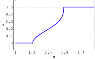
Figure 1: Solutions to the equation of motion for $\omega$. The blue (solid) line corresponds to a minimum while the red (dashed) one is a maximum.

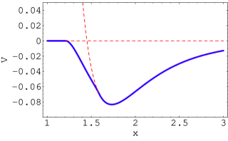
Figure 2: The Casimir energy for the different solutions of Fig. 1.

The precise values of $x_{0}$ and $x_{1}$ can be determined in the approximation (3.8) from

$$\delta F(x_{0})=3\zeta(3),$$ (3.10)

$$\delta F(x_{1})=\frac{9}{4}\zeta(3).$$ (3.11)

Furthermore we can approximate the sum in Eq. (3.8) by e.g. its first three terms which allows an analytic determination of $\omega(x)$ in the region $x_{0}\leq x\leq x_{1}$

$$\omega(x)=\frac{1}{2\pi}\arccos\left\{-\frac{81}{64}+\left[\left(\frac{81}{64}\right)^{2}-20+\frac{27}{4}\delta F(x)\right]^{\scriptstyle 1/2}\right\}.$$ (3.12)

The resulting Casimir energy $V(\omega(x),x)$ is plotted in Fig. 2. Notice that the minimum corresponds to $x>x_{1}$, i.e. to $\omega=\frac{1}{2}$. Also note that for $\delta\to 1$ the minimum disappears: this is easily seen from the exact behaviour of $f(1/2,x)$ for $x\to 0$, $x\to\infty$ which is given by

$$\lim_{x\to 0}f(1/2,x)=-12(1-\delta)\zeta(5),\qquad\lim_{x\to\infty}f(1/2,x)=-12\zeta(5).$$ (3.13)

This indicates that the function $x^{-6}f(1/2,x)$ only has a minimum for $\delta>1$.

In the presence of supersymmetry breaking brane effects the value of $\omega$ is fixed at tree level and the potential Eq. (3.6) (for $a=0$, $b=0$) has a minimum for any value of $\omega$. In Fig. 3 the Casimir energy is plotted for $\delta=1.5$ and several values of $\omega$. Similar arguments to those following Eq. (3.13) also lead, for arbitrary $\omega$, to radion stabilization only for $\delta>1$. Notice that for $x\geq x_{1}$, i.e. in the region of the minimum, the potential of Fig. 2 coincides with that of Fig. 3 for $\omega=\frac{1}{2}$. This means that for all practical purposes we can consider the potential Eq. (3.6) with $\omega$ constant (i.e. not depending on $x$) and the case of no supersymmetry breaking brane effects just corresponds to $\omega=\frac{1}{2}$.

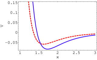
Figure 3: The Casimir energy for fixed $\omega=1/4$ (red/dashed line) and $\omega=1/2$ (blue/full line).

The potential corresponding to the Casimir energy should then be completed with the counterterm Lagrangian with $g^{2}>0$ and $T_{0},\,T_{\pi}>0$ to fine-tune to zero the 4D cosmological constant. In particular, the condition for supersymmetric AdS₅ space is [25]

$$T_{0,\pi}\leq\sqrt{6}gM_{5}^{3/2},$$ (3.14)

which translates in our case to

$$\frac{1}{4\pi}\frac{M}{M_{5}}\leq\left[\frac{6|a|}{(2+N_{V}-N_{h})\pi b^{2}}\right]^{1/3}.$$ (3.15)

When we include the counterterms $a<0$ and $b>0$ (fine-tuned to have a zero cosmological constant) the effective potential develops an extra AdS₄ minimum and goes to zero from below for $x\to\infty$. An example is shown in Fig. 4 where the effective potential corresponding to $\omega=1/2$ and $a=-0.05$ is presented.

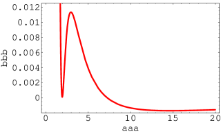
Figure 4: The effective potential corresponding to the $\omega=1/2$ case with fine-tuned counterterms.

In any case we should be concerned for the tunneling from the Minkowski to the AdS vacuum. In the rest of this section we will estimate the tunneling rate and find it to be exceedingly small so that our vacuum with zero cosmological constant is stable.

A priori, the quantum mechanical stability of the false Minkowski vacuum state is not guaranteed since the decay of the false vacuum into the AdS vacuum may proceed by quantum tunneling in a finite sized bubble. In order to estimate the tunneling probability, we use a dimensional argument . The kinetic term for the field $\phi$ assumes the form

$${\cal L}_{\rm kin}=\frac{1}{6}M_{4}^{2}\frac{\partial_{\mu}\phi\partial^{\mu}\phi}{\phi^{2}},$$ (3.16)

where $M_{4}$ is the four-dimensional Planck scale. The potential for the field $\phi$ can be generically written in the form $M^{4}{\cal V}(\phi)$, where ${\cal V}(\phi)$ is a dimensionless quantity. The equation for the flat space instanton which controls the tunneling rate from the false to the true vacuum is given by

$$\partial_{\rho}^{2}\phi_{\rm inst}+\frac{3}{\rho}\partial_{\rho}\phi_{\rm inst}-2\frac{\left(\partial_{\rho}\phi_{\rm inst}\right)^{2}}{\phi_{\rm inst}}=6\phi_{\rm inst}^{2}\frac{M^{4}}{M_{4}^{2}}\left.\frac{d{\cal V}}{d\phi}\right|_{\phi=\phi_{\rm inst}},$$ (3.17)

where $\phi_{\rm inst}=\phi_{\rm inst}(\rho)$ is the instanton solution. It is a function of the variable $\rho=\sqrt{\vec{x}^{2}+t^{2}}$ which makes the $SO(4)$ symmetry of instanton solutions at zero temperature manifest. The solution to Eq. (3.17) will have the form

$$\phi_{\rm inst}=f\left(z\frac{M_{4}}{M^{2}}\right),$$ (3.18)

where $z$ is a dimensionless variable. Eq. (3.18) tells us that the critical size $\rho_{c}$ of the bubble by which tunneling may proceed is of the order of

$$\rho_{c}\sim\frac{M_{4}}{M^{2}}.$$ (3.19)

As a consequence it is easy to see that the instanton action is of the order of

$$S_{\rm inst}\sim\rho_{c}^{4}\,M^{4}{\cal V}\sim\left(\frac{M_{4}}{M}\right)^{4}.$$ (3.20)

The corresponding vacuum tunneling probability per unit space-time volume is of the order of

$${\cal P}\sim e^{-S_{\rm inst}}\sim e^{-10^{60}},$$ (3.21)

where in the last passage we have chosen $M\sim$ 1 TeV. This is so small that the false vacuum is essentially stable on cosmological times.

At this stage the reader might wonder why the tunneling probability is so small and be puzzled by the fact that decreasing the size of the barrier separating the false from the true vacuum by lowering $M$, the tunneling probability drops exponentially. The reason is the following: in terms of the field $\sigma=\frac{M_{4}}{\sqrt{3}}\,{\rm ln}\,\phi$ which canonically normalizes the kinetic term (3.16), the height of the barrier separating the two vacua is of the order of $M^{4}$, while the two vacua are far from each other at a distance $\sim M_{4}\gg M$ in field space. Despite the small barrier between the two vacua, in order to tunnel a macroscopic bubble has to be nucleated. Indeed, the smaller the barrier the bigger the size of the bubble, $\rho_{c}\sim\frac{M_{4}}{M^{2}}$. This amounts to saying that, despite the small energy-density $\sim M^{4}$ inside the bubble, its radius is so large that the total energy cost is measured by $M^{4}\rho_{c}^{4}$ which is precisely of the order of $S_{\rm inst}$ in Eq. (3.20).

4 Conclusion and Outlook

In this paper we have addressed the issue of radion stabilization in supersymmetric five-dimensional theories compactified on the orbifold $S^{1}/\mathbb{Z}_{2}$ where supersymmetry is broken by the Scherk-Schwarz mechanism. SS supersymmetry breaking can be straightforwardly implemented in the off-shell version of 5D supergravity using tensor- or linear multiplets as compensators. We have shown in detail that both formulations are equivalent both locally and globally and that a one loop analysis is needed to fix the supersymmetry breaking flux for the auxiliary gauge field of the $U(1)_{R}$ automorphism symmetry. In a globally inequivalent version, the linear multiplet formulation allows for a tree level breaking of supersymmetry [21]. We have shown that the bulk radius may be stabilized in the presence of a number $N_{H}$ of quasi-localized bulk fields whose contribution to the one-loop Casimir energy is such that, once introduced a bulk cosmological constant and brane tensions to achieve zero four-dimensional cosmological constant, the radion field is stabilized in a metastable Minkowski vacuum. For the mechanism to work we have found a lower bound on $N_{H}$ given by $2+N_{V}+N_{h}$ where $N_{V}$ $(N_{h})$ is the number of massless gauge multiplets (hypermultiplets) propagating in the bulk. We have shown that the probability of decaying from such a vacuum to the true one with negative cosmological constant is completely negligible.

In the metastable vacuum the squared mass of the canonically normalized radion field is given by $\sim$ (one-loop factor)$\times\frac{M^{4}}{M_{4}^{2}}$. Since the size of the odd-mass term $M$ may be taken to be of the order of 10 TeV, we conclude that the radion field acquires in the metastable vacuum a mass around $(10^{-3}-10^{-2})$ eV. This range of masses is interesting for present and future measureaments of deviations from the gravitational inverse-square law in the millimeter range [35].

We should also comment at this point about the relationship of radion stabilization with the hierarchy problem. Unlike in those approaches where a warped geometry solves the hierarchy problem, in flat space we must invoke supersymmetry for solving it. Therefore even if solving the hierarchy problem by the radion stabilization in warped geometries was a real issue, here it is not such. Our only concern was to obtain a physical radius $\stackrel{{\scriptstyle<}}{{{}_{\sim}}}1/$TeV. However this range is technically natural since we are introducing bulk masses in the TeV range. A different (not unrelated) issue is the origin of the weakness of gravitational interactions in the 4D theory and its relation with radion fixing. Here we have been working in a 5D gravity theory, with a 1/TeV length radius, and therefore the presence of submillimeter dimensions is not consistent with our mechanism for radion stabilization. On the other hand the relation between the Planck scales in the 4D and 5D theories, $M_{4}^{2}=M_{5}^{3}R$, with $R\sim 1/$TeV implies that the scale where gravity becomes strong in the 5D theory is much higher than $1/R$. This means that gauge interactions of the 5D theory become non-perturbative at a scale $M_{s}\ll M_{5}$ in the multi-TeV range. The theory should then have a cutoff at the scale $M_{s}$ where a more fundamental theory should be valid. An example of such behaviour is provided by Little String Theories (LST) at the TeV [36, 37] where the string coupling $g_{s}\ll 1$ and $M_{s}$ and $M_{5}$ are related by $M_{5}^{3}=M_{s}^{3}/g_{s}^{2}$. In other words $M_{5}$ does no longer play the role of a fundamental field theoretical cutoff scale. In these theories the weakness of the gravitational interactions is provided by the smallness of the string coupling. Moreover a class of LST has been found [37] where the Yang-Mills coupling is not provided by the string coupling but by the geometry of the compactified space where gauge interactions are localized, e.g. $g_{YM}\sim\ell_{s}/R$. Since the field theory has a cutoff at $M_{s}$ the consistency of the whole picture relies on the assumption that there is a wide enough range where the 5D field theory description is valid.

Finally, we should also be concerned about the backreaction of the Casimir energy and the counterterms on the originally flat 5D gravitational background. A dimensional analysis shows that the effect of the counterterms by themselves would result in a warp factor with a functional dependence on the extra coordinate as $a(\epsilon My)$, where $\epsilon=\mathcal{O}(M/M_{5})^{3/2}\equiv\mathcal{O}(M/M_{4})\sim 10^{-15}$ for $M\sim$ TeV. Such a warping is competely negligible. One can also show that the size of the gravitino bulk and brane masses generated by the counterterms are of the order of the radion mass and thus negligible as compared to the size of supersymmetry breaking contributions.

Acknowledgments

This work was supported in part by the RTN European Programs HPRN-CT-2000-00148 and HPRN-CT-2000-00152, and by CICYT, Spain, under contracts FPA 2001-1806 and FPA 2002-00748. The work of one of us (G.v.G.) is supported by the DAAD. Another of us (A.R.) would like to thank the Theory Department of IFAE, where part of this work has been done, for hospitality. We would like to thank J. Garriga and O. Pujolas for discussions.

References

- [1] I. Antoniadis, Phys. Lett. B246 (1990) 377; I. Antoniadis, C. Muñoz and M. Quirós, Nucl. Phys. B397 (1993) 515; I. Antoniadis and K. Benakli, Phys. Lett. B326 (1994) 69; I. Antoniadis, K. Benakli and M. Quirós, Phys. Lett. B331 (1994) 313; I. Antoniadis and M. Quirós, Phys. Lett. B392 (1997) 61.
- [2] P. Horava and E. Witten, Nucl. Phys. B460 (1996) 506 [hep-th/9510209]; P. Horava and E. Witten, Nucl. Phys. B475 (1996) 94 [hep-th/9603142]; P. Horava, Phys. Rev. D54 (1996) 7561 [hep-th/9608019].
- [3] I. Antoniadis and M. Quiros, Nucl. Phys. B505 (1997) 109 [hep-th/9705037]; I. Antoniadis and M. Quiros, Phys. Lett. B416 (1998) 327 [hep-th/9707208]; I. Antoniadis and M. Quiros, Nucl. Phys. Proc. Suppl. 62 (1998) 312 [hep-th/9709023].
- [4] H. P. Nilles, M. Olechowski and M. Yamaguchi, Phys. Lett. B415 (1997) 24 [hep-th/9707143]; H. P. Nilles, M. Olechowski and M. Yamaguchi, Nucl. Phys. B530, 43 (1998) [hep-th/9801030]; H. P. Nilles, hep-ph/0004064.
- [5] E. A. Mirabelli and M. E. Peskin, Phys. Rev. D58 (1998) 065002 [hep-th/9712214].
- [6] J. R. Ellis, Z. Lalak, S. Pokorski and W. Pokorski, Nucl. Phys. B540 (1999) 149 [hep-ph/9805377].
- [7] L. Randall and R. Sundrum, Nucl. Phys. B557 (1999) 79 [hep-th/9810155].
- [8] A. Pomarol and M. Quirós, Phys. Lett. B438 (1998) 255; I. Antoniadis, S. Dimopoulos, A. Pomarol and M. Quiros, Nucl. Phys. B544 (1999) 503 [hep-ph/9810410]; A. Delgado, A. Pomarol and M. Quiros, Phys. Rev. D60 (1999) 095008 [hep-ph/9812489].
- [9] D. E. Kaplan, G. D. Kribs and M. Schmaltz, Phys. Rev. D62 (2000) 035010 [hep-ph/9911293]; Z. Chacko, M. A. Luty, A. E. Nelson and E. Ponton, JHEP 0001 (2000) 003 [hep-ph/9911323].
- [10] T. Gherghetta and A. Pomarol, Nucl. Phys. B602 (2001) 3 [hep-ph/0012378].
- [11] J. Scherk and J. H. Schwarz, Phys. Lett. B82 (1979) 60; ibidem, Nucl. Phys. B153 (1979) 61.
- [12] G. von Gersdorff and M. Quiros, Phys. Rev. D65 (2002) 064016 [hep-th/0110132].
- [13] H. Georgi, A. K. Grant and G. Hailu, Phys. Rev. D63 (2001) 064027 [hep-ph/0007350]; N. Arkani-Hamed, A. G. Cohen and H. Georgi, Phys. Lett. B516 (2001) 395 [hep-th/0103135].
- [14] D. M. Ghilencea, S. Groot Nibbelink and H. P. Nilles, Nucl. Phys. B619 (2001) 385 [hep-th/0108184].
- [15] R. Barbieri, R. Contino, R. Creminelli, R. Rattazzi and C. A. Scrucca Phys. Rev. D66 (2002) 024025 [hep-th/0203039]; D. Marti and A. Pomarol, Phys. Rev. D66 (2002) 125005 [hep-ph/0205034].
- [16] M. Zucker, Nucl. Phys. B570 (2000) 267 [hep-th/9907082]; JHEP 0008 (2000) 016 [hep-th/9909144]; Phys. Rev. D64 (2001) 024024 [hep-th/0009083].
- [17] M. Zucker, Fortsch. Phys. 51 (2003) 899.
- [18] Z. Lalak and R. Matyszkiewicz, Nucl. Phys. B649 (2003) 389 [hep-th/0210053].
- [19] J. Bagger and M. Redi, hep-th/0310086.
- [20] G. von Gersdorff, M. Quiros and A. Riotto, Nucl. Phys. B634 (2002) 90 [hep-th/0204041].
- [21] R. Rattazzi, C. A. Scrucca and A. Strumia, hep-th/0305184.
- [22] B. de Wit, R. Philippe and A. Van Proeyen, Nucl. Phys. B219 (1983) 143.
- [23] J. Bagger, F. Feruglio and F. Zwirner, JHEP 0202 (2002) 010 [hep-th/0108010].
- [24] K. A. Meissner, H. P. Nilles and M. Olechowski, Acta Phys. Polon. B33 (2002) 2435 [hep-th/0205166].
- [25] J. Bagger and D. V. Belyaev, Phys. Rev. D67 (2003) 025004 [hep-th/0206024].
- [26] A. Delgado, G. von Gersdorff and M. Quiros, JHEP 0212 (2002) 002 [hep-th/0210181].
- [27] Z. Lalak and R. Matyszkiewicz, Phys. Lett. B562 (2003) 347 [hep-th/0303227].
- [28] K. Y. Choi and H. M. Lee, hep-th/0306232.
- [29] I. L. Buchbinder, S. J. Gates, H. S. Goh, W. D. Linch, M. A. Luty, S. P. Ng and J. Phillips, hep-th/0305169.
- [30] J. Bagger and D. Belyaev, JHEP 0306 (2003) 013 [hep-th/0306063].
- [31] T. Appelquist and A. Chodos, Phys. Rev. Lett. 50 (1983) 141. T. Appelquist and A. Chodos, Phys. Rev. D28 (1983) 772.
- [32] E. Ponton and E. Poppitz, JHEP 0106 (2001) 019 [hep-ph/0105021].
- [33] G. von Gersdorff, L. Pilo, M. Quiros, D. A. Rayner and A. Riotto, [hep-ph/0305218].
- [34] S. R. Coleman and F. De Luccia, Phys. Rev. D21, 3305 (1980).
- [35] E. G. Adelberger, B. R. Heckel and A. E. Nelson, hep-ph/0307284.
- [36] O. Aharony, Class. Quant. Grav. 17 (2000) 929 [hep-th/9911147].
- [37] I. Antoniadis, S. Dimopoulos and A. Giveon, JHEP 0105 (2001) 055 [hep-th/0103033].