hep-th/0310173

FSU-TPI-08/03


Effective Supergravity Actions for Flop Transitions 111Work supported by the ‘Schwerpunktprogramm Stringtheorie’ of the DFG.


Laur Järv, Thomas Mohaupt and Frank Saueressig

Institute of Theoretical Physics, Friedrich-Schiller-University Jena,
Max-Wien-Platz 1, D-07743 Jena, Germany
L.Jaerv, T.Mohaupt, F.Saueressig@tpi.uni-jena.de


ABSTRACT

We construct a family of five-dimensional gauged supergravity actions which describe flop transitions of M-theory compactified on Calabi-Yau threefolds. While the vector multiplet sector can be treated exactly, we use the Wolf spaces $X(1+N)=\frac{U(1+N,2)}{U(1+N)\times U(2)}$ to model the universal hypermultiplet together with $N$ charged hypermultiplets corresponding to winding states of the M2-brane. The metric, the Killing vectors and the moment maps of these spaces are obtained explicitly by using the superconformal quotient construction of quaternion-Kähler manifolds. The inclusion of the extra hypermultiplets gives rise to a non-trivial scalar potential which is uniquely fixed by M-theory physics.

1 Introduction

Supergravity actions provide a powerful tool for studying the low energy dynamics of string and M-theory compactified on special holonomy manifolds. In this case one usually has a moduli space of vacua, corresponding to the deformations of the internal manifold $X$ and the background fields. For theories with eight or less supercharges this moduli space includes special points where $X$ becomes singular, leading to a discontinuous or singular low energy effective action (LEEA). However, within the full string or M-theory these singularities are believed to be artifacts, which result from ignoring some relevant modes of the theory, namely the winding states of strings or branes around the cycles of $X$. Singularities of $X$ arise when such cycles are contracted to zero volume, which leads to additional massless states. It was the crucial insight of [1] that the singularities occurring in the LEEA of type II strings compactified on a Calabi-Yau (CY) threefold with a conifold singularity can be interpreted as arising from illegitimately integrating out such massless states. This has been generalized to many other situations, including M-theory compactifications on CY threefolds [2]. In some cases it is possible to resolve the singularity of $X$ in two or more topologically different ways. This gives rise to so-called topological phase transitions. Such transitions have been studied intensively in literature [3, 4, 5, 2].222We refer to [6] for a review and more references. They can be realized as parametric deformations of vacua, but also dynamically [7, 8, 9, 10, 11].

The usual LEEA only include those states which are generically massless, while the extra light modes occurring in a topological phase transition are left out. We refer to this description as the ‘Out-picture’. For the complete description of the low energy physics, however, one also needs to include the additional light modes. Following [10], we will call these additional light modes ‘transition states’. The low energy description which explicitly includes the transition states will be referred to as the ‘In-picture’.

There are various reasons why it is important to know the In-picture description of topological phase transitions. The compactification of type II string theory or M-theory on smooth spaces gives rise to a massless spectrum which only contains neutral states. However, in the vicinity of special points one can get non-abelian gauge groups and charged chiral matter, which makes such compactifications viable for particle physics model building. Since in these models all charged particles are transition states, it is clear that one needs the extended LEEA corresponding to the In-picture to describe their dynamics. It has also been shown that in compactifications with background flux the scalar potential has its minima at special points in moduli space, where additional light states occur [12, 13]. Conversely, it has been noticed in [10] that even in the absence of flux the potential generated by the transition states has the effect that the region in the vicinity of a topological phase transition is dynamically preferred. Finally, there is some evidence that the interplay between singularities and background flux generates a small scale, which could help to solve the gauge hierarchy and the cosmological constant problem [14, 15, 16].

Although it is clear in principle that one should be able to “integrate in” the additional states, not much effort has been devoted towards working out the corresponding LEEA explicitly. A systematic investigation was started in [17] and continued in [18], by deriving the explicit LEEA which describe $SU(2)$ gauge symmetry enhancement through string or brane winding states in five and four dimensions. For compactifications with ${\cal N}=4$ supersymmetry (16 supercharges) non-abelian gauge symmetry enhancement of the LEEA has been considered in [19].

The first step to obtain analogous results for flop transitions occurring in M-theory compactified on CY threefolds has been made in [10]. In this case the transition states are given by charged hypermultiplets which combine with the neutral hypermultiplets arising from the smooth CY compactification. Local supersymmetry requires that these fields parametrize a non-flat quaternion-Kähler manifold [20]. In [10] the difficulties in working with these rather complicated manifolds were avoided by taking the hypermultiplet manifold to be flat. This, however, is only compatible with global supersymmetry and does not give rise to a consistent supergravity description of the transition.

In this paper we construct In-picture LEEA for flop transitions which are $\mathcal{N}=2$ locally supersymmetric. The strategy is to combine information about the transition states coming from M-theory with knowledge about the general $\mathcal{N}=2,D=5$ gauged supergravity action [21, 22, 23, 24].333Here ${\cal N}$ counts real supercharges in multiples of 4. Thus ${\cal N}=2$ refers to the smallest supersymmetry algebra in five dimensions.

As long as the CY threefold $X$ is smooth, the LEEA can be obtained by dimensional reduction [25]. Besides the five-dimensional supergravity multiplet, it contains vector and hypermultiplets whose couplings are determined by $X$. The LEEA is an ungauged supergravity action: all fields are neutral, the gauge group is abelian, and there is no scalar potential. In a flop transition the Kähler moduli are varied such that $X$ becomes singular through the contraction of $N$ isolated holomorphic curves [2]. The winding states of M2-branes around these curves give rise to $N$ charged hypermultiplets, which become massless at the transition locus. These are the transition states that we want to integrate in. Since they are charged, the resulting action is a gauged supergravity action, which has a non-trivial scalar potential.

The vector multiplet sector of the LEEA contains the Kähler moduli which control the sizes of the $N$ holomorphic curves and, hence, the phase transition. These parametrize a so-called very special real manifold which is completely determined by a cubic polynomial, the prepotential. In the Out-picture the prepotential can be computed exactly and the threshold corrections arising from integrating out the transition states have been derived in [2]. As a result, we can determine the vector multiplet part of the In-picture LEEA exactly.

The situation is much more complicated in the hypermultiplet sector, and this is the main point we have to address in this paper. Local supersymmetry requires that the hypermultiplet manifold is a quaternion-Kähler manifold with non-trivial Ricci curvature [20]. The latter constraint excludes hyper-Kähler and in particular flat manifolds. The main difference between (generic) quaternion-Kähler manifolds and other geometries familiar from supersymmetric theories, such as hyper-Kähler and special Kähler manifolds, is that there are no simple, globally defined holomorphic objects which encode the information one needs to construct the LEEA. There is no Kähler potential and in general a quaternion-Kähler manifold is not even a complex manifold. Moreover, for the study of gaugings it would be convenient to take the hypermultiplet manifold to be a direct product, with the neutral fields in one factor and the charged fields in the other. But this is also not an option, because the product of two (generic) quaternion-Kähler manifolds is not quaternion-Kähler.

Due to these complications, this type of geometry is much less understood than the other geometries occurring in supergravity. In particular, only very limited results exist on how to explicitly compute the hypermultiplet metric in string or M-theory. The best studied subsector is the universal hypermultiplet, which at tree level is described by the coset $\frac{U(1,2)}{U(1)\times U(2)}$, but receives a non-trivial loop correction [26]. The tree level result for the neutral hypermultiplets can be obtained through the c-map [27, 28], but only little is known about quantum corrections (see [29] for a review). Charged multiplets have not been studied at all.

Therefore we take the approach of using a toy model: to describe a flop transition we use a particular family of symmetric quaternion-Kähler spaces, the non-compact versions of the unitary Wolf spaces

$$X(1+N)=\frac{U(1+N,2)}{U(1+N)\times U(2)}\,,$$ (1.1)

containing $N+1$ hypermultiplets. One of these hypermultiplets will be identified with the universal hypermultiplet while the $N$ other hypermultiplets will correspond to the transition states. Their charges are determined by the geometry of the flop transition. The remaining neutral hypermultiplets present in a generic LEEA will be ignored. This is a reasonable approximation, because these hypermultiplets parametrize the complex structure of $X$, which is kept fixed in a flop transition. As we will show, this input suffices to uniquely determine the gauging and, hence, the remaining freedom in the LEEA which then indeed has all the properties required to model a flop. Only the transition states acquire a mass away from the transition locus, and the potential has a family of degenerate supersymmetric Minkowski ground states, which is parametrized by the moduli of $X$.

In order to cope with the technical problems arising in the hypermultiplet sector it is extremely useful that every quaternion-Kähler manifold can be obtained from a so-called hyper-Kähler cone by a superconformal quotient [30]. As indicated by the name, this construction is intimately related to the construction of hypermultiplet actions using the superconformal tensor calculus [31, 32, 33]. This treatment does not utilize the fact that the spaces $X(1+N)$ happen to be Kähler, but only relies on techniques which apply to any quaternion-Kähler manifold. Moreover, working on the level of the hyper-Kähler cone has the advantage that the product of two hyper-Kähler cones is again a hyper-Kähler cone. Thus one can put all the neutral fields in a separate factor. The isometries of $X(1+N)$ are also obtained from the isometries of the corresponding hyper-Kähler cone. We find the resulting parametrization very useful for discussing the gauging of the LEEA, as it is straightforward to see which Killing vector corresponds to the gauging describing a flop transition. The standard parametrization of $X(1+N)$ [28], which relies on its Kähler structure, is much less useful for this.

The remaining sections of this paper are organized as follows. In section 2 we review the general $\mathcal{N}=2,D=5$ gauged supergravity action and its relation to CY compactifications of M-theory. We explain how the vector multiplet sector can be determined exactly and introduce an explicit model for a flop transition. In section 3 we use the superconformal quotient construction to derive the metric and all isometries of the unitary Wolf spaces $X(1+N)$. In section 4 we construct an LEEA for the specific flop model introduced in subsection 2.3, which explicitly includes the transition states. In section 5 we generalize this setup to a generic flop transition and show that our input uniquely fixes the hypermultiplet sector of the In-picture Lagrangian. In section 6 we discuss our results and give an outlook on future research.

2 Five-dimensional Supergravity and Calabi-Yau compactifications

First we will review the relevant properties of $\mathcal{N}=2$, $D=5$ gauged supergravity [21, 22, 23, 24] and its relation to M-theory compactified on CY threefolds. For smooth CY compactifications this relation was worked out in [25]. Our conventions for the five-dimensional gauged supergravity action follow [34]. We refer to these papers for further details.

2.1 Five-dimensional gauged supergravity

The LEEA of eleven-dimensional supergravity compactified on a smooth CY threefold $X$ with Hodge numbers $h^{p,q}$ is given by five-dimensional supergravity coupled to $n_{V}=h^{1,1}-1$ abelian vector and $n_{N}=h^{2,1}+1$ neutral hypermultiplets. By explicitly including the transition states arising in a flop transition we additionally obtain $\delta n_{H}$ charged hypermultiplets.

The natural starting point for the construction of a LEEA which includes these states is given by the general $\mathcal{N}=2,D=5$ gauged supergravity action with $n_{V}$ vector, $n_{H}=n_{N}+\delta n_{H}$ hyper and no tensor multiplets. Anticipating the results of sections 4 and 5, we limit ourselves to the case of abelian gaugings. The bosonic matter content of this theory consists of the graviton $e_{\mu}^{~{}a}$, $n_{V}+1$ vector fields $A^{I}_{\mu}$ with field strength $F_{\mu\nu}^{I}=\partial_{\mu}A^{I}_{\nu}-\partial_{\nu}A^{I}_{\mu}$, $n_{V}$ real vector multiplet scalars $\phi^{x}$, and $4n_{H}$ real hypermultiplet scalars $q^{X}$. The bosonic part of the Lagrangian reads:

$\displaystyle\sqrt{-g}^{-1}\mathcal{L}^{\mathcal{N}=2}_{\rm bosonic}$ $\displaystyle=$ $\displaystyle-\frac{1}{2}R-\frac{1}{4}a_{IJ}F^{I}_{\mu\nu}F^{J~{}\mu\nu}$
$\displaystyle-\frac{1}{2}g_{XY}\mathcal{D}_{\mu}q^{X}\mathcal{D}^{\mu}q^{Y}-\frac{1}{2}g_{xy}\mathcal{D}_{\mu}\phi^{x}\mathcal{D}^{\mu}\phi^{y}$
$\displaystyle+\frac{1}{6\sqrt{6}}C_{IJK}\sqrt{-g}^{-1}\epsilon^{\mu\nu\rho\sigma\tau}F^{I}_{\mu\nu}F^{J}_{\rho\sigma}A^{K}_{\tau}-{\rm g}^{2}\mathbbm{V}(\phi,q)\,.$

The scalars $\phi^{x}$ and $q^{X}$ parametrize a very special real manifold $\mathcal{M}_{\mbox{\scriptsize VM}}$ [21] and a quaternion-Kähler444In parts of the physical literature, including [20], these manifolds are called ‘quaternionic’. However, in the mathematical literature quaternionic is a weaker condition than ‘quaternion(ic)-Kähler’. Definitions for both kinds of manifolds are given later in the main text. manifold $\mathcal{M}_{\mbox{\scriptsize HM}}$ with Ricci scalar ${\cal R}=-8n_{H}(n_{H}+2)$ [20], respectively.

The vector multiplet sector is determined by the completely symmetric tensor $C_{IJK}$, appearing in the Chern-Simons term. This tensor is used to define a real homogeneous cubic polynomial

$${\cal V}(h)=C_{IJK}\,h^{I}\,h^{J}\,h^{K}\,$$ (2.2)

in $n_{V}+1$ real variables $h^{I}$. The $n_{V}$-dimensional manifold ${\cal M}_{\mbox{\scriptsize VM}}$ is obtained by restricting this polynomial to the hypersurface

$${\cal V}(\phi)=C_{IJK}\,h^{I}(\phi)\,h^{J}(\phi)\,h^{K}(\phi)=1\,.$$ (2.3)

The coefficients $a_{IJ}$ appearing in the kinetic term of the vector field strength are given by

$$\begin{split}a_{IJ}(h)&:=-\,\left.\frac{1}{3}\,\frac{\partial}{\partial h^{I}}\,\frac{\partial}{\partial h^{J}}\,\ln{\cal V}(h)\right|_{{\cal V}=1}\\ &=-2\,C_{IJK}\,h^{K}+3\,C_{IKL}\,C_{JMN}\,h^{K}h^{L}h^{M}h^{N}\,.\end{split}$$ (2.4)

Defining

$$h^{I}_{x}:=-\,\sqrt{\frac{3}{2}}\,\frac{\partial}{\partial\phi^{x}}\,h^{I}(\phi)\,,\quad h_{I}:=C_{IJK}h^{J}h^{K}\,,$$ (2.5)

the metric on $\mathcal{M}_{\mbox{\scriptsize VM}}$ is proportional to the pullback555The $a_{IJ}$ can be interpreted as a metric on the space into which ${\cal M}_{\mbox{\scriptsize VM}}$ is immersed by (2.3). of $a_{IJ}$,

$$g_{xy}(\phi):=h^{I}_{x}\,h^{J}_{y}\,a_{IJ}\,.$$ (2.6)

The hypermultiplet scalars $q^{X}$ parametrize a quaternion-Kähler manifold of dimension $\dim_{\mathbbm{R}}(\mathcal{M}_{\mbox{\scriptsize HM}})=4n_{H}$. For $n_{H}>1$ such manifolds are characterized by their holonomy group,

$$Hol(\mathcal{M}_{\mbox{\scriptsize HM}})=SU(2)\cdot USp(2n_{H})\,,$$ (2.7)

while in the case $n_{H}=1$ they are defined as Einstein spaces with self-dual Weyl curvature. The restricted holonomy group implies that the curvature tensor decomposes into an $SU(2)$ and $USp(2n_{H})$ part

$$R_{XYWZ}\,f^{W}_{iA}\,f^{Z}_{jB}=\epsilon_{ij}\,R_{XYAB}+C_{AB}\,R_{XYij}\,.$$ (2.8)

Here $i=1,2$ is an $SU(2)$ index and $A=1,\ldots,2n_{H}$ is a $USp(2n_{H})$ index. These are raised and lowered by the symplectic metrics $\epsilon_{ij}$ and $C_{AB}$, respectively. The $4n_{H}$-bein $f^{iA}_{X}$ is related to the metric on $\mathcal{M}_{\mbox{\scriptsize HM}}$ by

$$g_{XY}=f_{X}^{iA}f^{jB}_{Y}\epsilon_{ij}C_{AB}=f^{iA}_{X}\,f_{YiA}\,,$$ (2.9)

and satisfies:

$$f^{X}_{iA}\,f^{iA}_{Y}=\delta^{~{}X}_{Y}\,,\quad f^{X}_{iA}f^{jB}_{X}=\delta_{i}^{~{}j}\delta_{A}^{~{}B}\,.$$ (2.10)

Local supersymmetry requires the $SU(2)$ part of the curvature to be non-vanishing [20]. This feature excludes hyper-Kähler manifolds as target manifolds, since these have trivial $SU(2)$ curvature.

The superconformal quotient construction [31, 32] employed in the next section provides a method to obtain all the quantities of interest in the hypermultiplet sector. In this approach the metric $g_{XY}$ and all its isometries are computed from the corresponding quantities of the associated hyper-Kähler cone, without the need to introduce the vielbein $f^{iA}_{X}$. However, to be able to relate our results to the mayor part of the literature on hypermultiplets, we review the properties of quaternion-Kähler manifolds using the vielbein $f^{iA}_{X}$.

We first introduce the Levi-Civita connection $\Gamma_{YZ}^{~{}~{}~{}X}$, a $USp(2n_{H})$ connection $\omega_{XB}^{~{}~{}~{}A}$, and an $SU(2)$ connection $\omega_{Xk}^{~{}~{}~{}i}$. The vielbein is covariantly constant with respect to these connections,

$$\partial_{X}f^{iA}_{Y}-\Gamma_{XY}^{~{}~{}~{}Z}f^{iA}_{Z}+f^{iB}_{Y}\omega_{XB}^{~{}~{}~{}A}+\omega_{Xk}^{~{}~{}~{}i}f^{kA}_{Y}=0\,.$$ (2.11)

The $SU(2)$ curvature can be expressed in terms of the vielbein as

$$\mathcal{R}_{XYij}=f_{XC(i}\,f^{C}_{j)Y}\,.$$ (2.12)

Raising the index $j$ with $\epsilon^{ij}$, we can expand the $SU(2)$ curvature in terms of the standard Pauli matrices,

$$\mathcal{R}_{XYi}^{~{}~{}~{}~{}~{}j}=i\,\mathcal{R}^{r}_{XY}\,\left(\sigma_{r}\right)_{i}^{~{}j}\,,$$ (2.13)

where $r=1,2,3$ enumerates the Pauli matrices. The $\mathcal{R}^{r}_{XY}$ defined in this way are real and satisfy

$$\mathcal{R}^{r}_{XY}\,\mathcal{R}^{sYZ}=-\,\frac{1}{4}\delta^{rs}\delta_{X}^{~{}Z}-\frac{1}{2}\,\epsilon^{rst}\mathcal{R}_{X}^{t~{}Z}\,.$$ (2.14)

It is no accident that the above formula resembles the quaternionic algebra. A quaternion-Kähler manifold is in particular quaternionic, i.e., there locally exists a triplet of almost complex structures, which satisfy the quaternionic algebra. The curvatures $\mathcal{R}^{r}_{XY}$ are proportional to these almost complex structures. However, since in general none of these almost complex structures is integrable, a quaternion-Kähler manifold does not need to be Kähler, or, in fact, not even complex.

We now turn to the isometries of ${\cal M}_{\mbox{\scriptsize HM}}$ which are relevant for the gauging. These must be compatible with the three locally defined almost complex structures, i.e., they leave the almost complex structures invariant up to an $SU(2)$ rotation. Such isometries are called tri-holomorphic. Given a tri-holomorphic Killing vector $K^{X}_{I}(q)$ on the quaternion-Kähler manifold, the $\mathcal{R}^{r}_{XY}$ can be used to construct an $SU(2)$ triplet of real prepotentials $P^{r}_{I}(q)$, the so-called moment maps [35]:666Up to a rescaling, these are identical to the $\hat{\mu}^{r}$ constructed in the next section.

$$\mathcal{R}^{r}_{XY}K^{Y}_{I}=D_{X}\,P^{r}_{I}\,,\quad D_{X}P^{r}_{I}:=\partial_{x}P^{r}_{I}+2\epsilon^{rst}\omega^{s}_{X}P^{t}_{I}\,.$$ (2.15)

Here $\omega^{s}_{X}$ is defined by $\omega_{Xi}^{~{}~{}~{}j}=:i\,\omega^{r}_{X}(\sigma_{r})^{~{}j}_{i}$. Using eq. (2.14) this relation can be solved for the Killing vector $K^{Y}_{I}(q)$:

$$K^{Z}_{I}=-\frac{4}{3}\mathcal{R}^{r~{}ZX}D_{X}P^{r}_{I}\,.$$ (2.16)

Hence the moment map $P^{r}_{I}$ provides a triplet of functions from which the Killing vectors of $\mathcal{M}_{\mbox{\scriptsize HM}}$ can be obtained. Additionally, one can show that eq. (2.15) determines the prepotentials uniquely. In particular, covariantly constant shifts $P^{r(0)}_{I}$ are excluded. This is shown by first contracting eq. (2.15) with $D_{X}$ and then using the harmonicity property of the prepotentials [36]:

$$P^{r}_{I}=\frac{1}{2n_{H}}D_{X}\left(K_{IY}\mathcal{R}^{r~{}XY}\right)\,.$$ (2.17)

By virtue of eq. (2.15), this relation implies $P^{r(0)}_{I}=0$ as $\mathcal{R}^{r}_{XY}K^{Y}_{I}=0$ for a covariantly constant shift. Hence there is no analog of $D=4$, $\mathcal{N}=1$ Fayet-Iliopoulos terms in $D=5$, $\mathcal{N}=2$ supergravity with a non-trivial hypermultiplet sector.

We now discuss the gauging of the Lagrangian (2.1). The scalars take values in a Riemannian manifold, and the gauge group must operate on them as a subgroup of the isometry group in order to keep the action invariant. The procedure which allows one to construct the gauge couplings is known as ‘gauging isometries of the scalar manifold’ [21, 22, 23, 24]. This procedure includes the covariantization of the derivatives appearing in the scalar kinetic terms with respect to isometries of the vector or hypermultiplet target manifolds,

$$\mathcal{D}_{\mu}q^{X}:=\partial_{\mu}q^{X}+{\rm g}A^{I}_{\mu}K^{X}_{I}(q)\,,\quad\mathcal{D}_{\mu}\phi^{x}:=\partial_{\mu}\phi^{x}+{\rm g}A^{I}_{\mu}K^{x}_{I}(\phi)\,.$$ (2.18)

Here the $K^{X}_{I}(q)$ and $K^{x}_{I}(\phi)$ are the Killing vectors of the gauged isometries in the hypermultiplet and vector multiplet scalar manifold, respectively. An important consequence of the gauging is that we now have a non-trivial scalar potential $\mathbbm{V}(\phi,q)$. Since we have both vector and hypermultiplets but no tensor multiplets, this potential is determined by the gauging of hypermultiplet isometries. In order to write down $\mathbbm{V}$ explicitly, we define:

$$P^{r}:=h^{I}(\phi)P^{r}_{I}\,,\quad P^{r}_{x}:=h^{I}_{x}P^{r}_{I}\,,\quad K^{X}:=h^{I}(\phi)K^{X}_{I}\,.$$ (2.19)

Here $h^{I}(\phi)$ are the scalars (2.2) associated to the gauge field $A^{I}_{\mu}$, $K_{I}^{X}(q)$ denotes the Killing vector of the hypermultiplet isometry for which $A^{I}_{\mu}$ serves as a gauge connection, and $P^{r}_{I}$ is its associated $SU(2)$ triplet of moment maps. The scalar potential takes the form

$$\mathbbm{V}(\phi,q)=-4P^{r}P^{r}+2g^{xy}P^{r}_{x}P^{r}_{y}+\frac{3}{4}g_{XY}K^{X}K^{Y}\;.$$ (2.20)

Under some conditions [34], this potential can be rewritten in terms of a real function ${\cal W}$. This ‘stability form’ is useful, because it is sufficient to guarantee the gravitational stability of the theory [37]. In five dimensions the relation between ${\cal W}$ and $\mathbbm{V}$ is:

$$\mathbbm{V}(\phi,q)=-6\mathcal{W}^{2}+\frac{9}{2}g^{\Lambda\Sigma}\partial_{\Lambda}\mathcal{W}\partial_{\Sigma}\mathcal{W}\,.$$ (2.21)

Here $\phi^{\Lambda}$, $\Lambda,\Sigma=1,\ldots n_{V}+4n_{H}$ denotes the combined set of vector and hypermultiplet scalar fields, $g^{\Lambda\Sigma}$ is the direct sum of the vector and hypermultiplet inverse metrics,

$$g^{\Lambda\Sigma}(\phi,q):=g^{XY}(q)\oplus g^{xy}(\phi)\,,$$ (2.22)

and $\mathcal{W}$ is given by

$$\mathcal{W}:=\sqrt{\frac{2}{3}\,P^{r}\,P^{r}}\,.$$ (2.23)

The equivalence of eqs. (2.20) and (2.21) requires that when splitting $P^{r}$ into its norm and phase,

$$P^{r}=\sqrt{\frac{3}{2}}\,\mathcal{W}\,Q^{r}\,,\quad Q^{r}\,Q^{r}=1\,,$$ (2.24)

the phase $Q^{r}$ is independent of the vector multiplet scalars, $\partial_{x}Q^{r}=0$. As we will show, the scalar potentials of our models indeed satisfy this condition, thereby guaranteeing that the vacua of the theory are stable.

2.2 Calabi-Yau compactifications

When compactifying eleven-dimensional supergravity on a smooth CY threefold $X$ [25], one obtains a five-dimensional ungauged supergravity action, i.e, all fields are neutral under the gauge group $U(1)^{n_{V}+1}$ and there is no scalar potential. In this case the objects introduced above acquire a geometrical interpretation: the vector multiplet scalars encode the deformations of the Kähler class of $X$ at fixed total volume, while the hypermultiplet scalars parametrize the volume of $X$, deformations of its complex structure, and deformations of the three-form gauge field. The hypermultiplet containing the volume is called the universal hypermultiplet, because it is insensitive to the complex structure of $X$. Further, the $C_{IJK}$ determining the vector multiplet sector of the LEEA are given by the triple intersection numbers of $X$,

$$C_{IJK}=D_{I}\cdot D_{J}\cdot D_{K}\;,$$ (2.25)

where the $D_{I}$, $I=0,\ldots,n_{V}$ are a basis of the homological four-cycles $H_{4}(X,\mathbbm{Z})$. The dual basis $C^{I}$ for the two-cycles is defined by

$$C^{I}\cdot D_{J}=\delta^{I}_{~{}J}\,.$$ (2.26)

By integrating the Kähler form over the two-cycles $C^{I}$ we obtain the quantities

$$\hat{h}^{I}=\int_{C^{I}}\,J\,,$$ (2.27)

which control the volumes of even-dimensional cycles of $X$. In particular, the overall volume of $X$ is given by

$$vol(X)=\frac{1}{3!}\int_{X}\,J\wedge J\wedge J={\textstyle\frac{1}{6}}C_{IJK}\hat{h}^{I}\hat{h}^{J}\hat{h}^{K}\,.$$ (2.28)

Since the modulus corresponding to the total volume belongs to the universal hypermultiplet, one needs to introduce rescaled fields

$$h^{I}=(6\,vol(X))^{-1/3}\,\hat{h}^{I}\,,$$ (2.29)

in order to separate the vector and hypermultiplet moduli [25, 10]. These rescaled moduli appear in the cubic polynomial (2.3). Moreover, one needs to split the volume into the volume modulus ${\rm V}$, which is a dynamical field, and a fixed reference volume ${\rm v}$, which relates the eleven-dimensional and the five-dimensional gravitational couplings,

$$vol(X)={\rm v\cdot V}\;,\;\;\;\mbox{where}\;\;\;{\textstyle\frac{{\rm v}}{\kappa_{(11)}^{2}}}={\textstyle\frac{1}{\kappa_{(5)}^{2}}}\;.$$ (2.30)

2.3 Flop transitions

We now review the geometry and M-theory physics of flop transitions. The discussion follows [2], but uses the terminology of [38]. Useful references for background information are [39, 6, 4].

The Kähler moduli space of a CY threefold $X$ is a cone, called the Kähler cone. The vector multiplet moduli space is the projectivization of this cone, or, equivalently, a hypersurface corresponding to fixed total volume. At the boundaries of the Kähler cone some submanifolds of $X$ contract to zero volume and $X$ becomes a singular CY space $\hat{X}$. If there is a second, inequivalent, way to resolve the singularities of $\hat{X}$, leading to a smooth but topologically different CY manifold $\tilde{X}$, then $X$ and $\tilde{X}$ are said to be related by a topological phase transition.

We will consider type I contractions, which lead to flop transitions. In this case the Kähler cones of $X$ and $\tilde{X}$ can be glued together along their common boundary $h^{\star}=0$. By joining the Kähler cones of all CY threefolds related by flops, one obtains the extended Kähler cone.

In a flop transition $N$ isolated holomorphic curves ${\cal C}_{i}$, $i=1,\ldots,N$, which belong to the same homology class $C^{\star}=q_{I}C^{I}$ and have volume $h^{\star}=q_{I}h^{I}$, are contracted to zero volume. By wrapping M2-branes around these holomorphic cycles, one obtains BPS states which carry the charges $\pm(q_{I})$, $I=0,\ldots,n_{V}$ under the gauge fields $A^{I}_{\mu}$. This means that these states are charged under the gauge group $U(1)\subset U(1)^{n_{V}+1}$, which corresponds to the gauge field $A_{\mu}^{\star}=q_{I}A^{I}_{\mu}$. Their masses are proportional to the volume of the holomorphic curves. By dimensional reduction of the M2-brane action one computes the mass [10]

$$M=T_{(2)}(6{\rm v})^{1/3}q_{I}h^{I}\;,$$ (2.31)

where $T_{(2)}$ is the tension of the M2-brane. Since $Z=\pm q_{I}h^{I}$ is the central charge of the charged states with respect to the five-dimensional supersymmetry algebra, we recognize the five-dimensional BPS mass formula $M_{(\mbox{\scriptsize BPS})}=\mbox{const}\cdot|Z|$.777 From the eleven-dimensional point of view the mass of a wrapped M2-brane is given by $M_{(11)}=T_{(2)}vol({\cal C})=T_{(2)}(6{\rm vV})^{1/3}q_{I}h^{I}$. However, the relation between the eleven-dimensional and five-dimensional metrics involves a conformal rescaling by the volume modulus ${\rm V}$.

For a flop transition these BPS-states are charged hypermultiplets, i.e., one obtains $N$ massless charged hypermultiplets at the boundary $h^{\star}=0$ of the Kähler cone of $X$. As long as the charged hypermultiplets have finite mass, $h^{\star}>0$, physics at scales below this mass can be described by the effective action $S$ derived from dimensional reduction on $X$. We call this the Out-picture LEEA, because it does not contain the transition states. Its vector multiplet sector is completely determined by the triple intersection numbers $C_{IJK}$. In the flop transition the curves ${\cal C}_{i}$ are contracted to zero volume and then re-expanded to holomorphic curves $\tilde{C}_{i}$ in the homology class $\tilde{C}^{\star}=-C^{\star}$. The triple intersection numbers $\tilde{C}_{IJK}$ of $\tilde{X}$ are related to those of $X$ by

$$\tilde{C}_{IJK}=C_{IJK}-\frac{N}{6}(D_{I}\cdot C^{\star})(D_{J}\cdot C^{\star})(D_{K}\cdot C^{\star})\;.$$ (2.32)

As long as the curves $\tilde{\cal C}_{i}$ have positive volume, they support $N$ charged hypermultiplets with finite mass proportional to $\tilde{h}^{\star}=-h^{\star}>0$. For energy scales below this mass we can use the standard LEEA $\tilde{S}$, obtained by dimensional reduction on $\tilde{X}$, whose vector multiplet sector is determined by the $\tilde{C}_{IJK}$. The actions $S$ and $\tilde{S}$ do not become singular in the limit $h^{\star}\rightarrow 0$.888 This is different in four dimensions, where the gauge couplings receive threshold corrections which depend logarithmically on the mass of the charged states which are integrated out. Therefore the actions $S$ and $\tilde{S}$ become singular at the transition locus and the use of an extended action $\hat{S}$ is indispensable. See [18] for an explicit example. Therefore one can in principle avoid to include the extra light modes and instead consider the coefficients $C_{IJK}$ as piecewise constant functions, which are discontinuous at the transition locus.

However, a complete low energy description in the vicinity of the boundary requires that we work with an extended LEEA, $\hat{S}$, which contains the transition states explicitly. The vector multiplet sector of $\hat{S}$ is completely determined by the coefficients $\hat{C}_{IJK}$ of its prepotential, which we would like to determine in terms of the $C_{IJK}$. To find this relation one notes that there is an intermediate regime, where the transition states have small, but non-vanishing masses. Here both the actions $\hat{S}$ and $S$ (or $\tilde{S}$) are valid. Therefore one can relate $\hat{S}$ to $S$ (or $\tilde{S}$) by integrating out the transition states. In the vector multiplet sector this can be done exactly. This result of [2] can be brought to a suggestive form by writing the $\hat{C}_{IJK}$ as ‘averaged triple intersection numbers’ [17],

$$\hat{C}_{IJK}={\textstyle\frac{1}{2}}\left(C_{IJK}+\tilde{C}_{IJK}\right)\;,$$ (2.33)

where $C_{IJK}$ and $\tilde{C}_{IJK}$ are related by (2.32). The change $C_{IJK}\rightarrow\tilde{C}_{IJK}$ can be viewed as a threshold effect resulting from integrating in the extra hypermultiplets at $h^{\star}>0$, continuing to $h^{\star}<0$ and then integrating them out again. We remark that it does not make sense to use the extended action $\hat{S}$ far away from the flop line, where the transition states have a considerable mass, because the full M-theory contains many other massive states which are not included in $\hat{S}$. Moreover, there are additional boundaries of the Kähler cones of $X$ and $\tilde{X}$, where some other states become massless.

So far we have seen that the vector multiplet sector of $\hat{S}$ can be determined exactly. In the hypermultiplet sector, however, one has the problem that it is very hard to compute the quaternion-Kähler metric on ${\cal M}_{\mbox{\scriptsize HM}}$ using string or M-theory. The main result of this paper is that one can find a gauged supergravity action with $N$ charged hypermultiplets which at least has all the qualitative properties required of $\hat{S}$. This derivation will be the subject of the sections 3 – 5.

Let us conclude with some remarks. For CY threefolds constructed using toric methods, the basic two-cycles $C^{I}$ can be chosen such that the Kähler cone of $X$ is given by $h^{I}>0$ [40]. We will call this the ‘adapted parametrization’. Then the collapse of a curve at the boundary $h^{J}=0$ is described by setting $q_{I}=\delta_{IJ}$ in the above formulae. This leads to some simplifications, as we have $h^{\star}=h^{J}$, $C^{\star}=C^{J}$, $A^{\star}_{\mu}=A^{J}_{\mu}$, etc. We will not assume the existence of such a parametrization in our general discussions, and only use it in the particular example introduced in the next subsection.

There are also other types of singularities which can occur at the boundaries of the Kähler cone. The only other cases involving finitely many transition states are the type III contractions, which lead to $SU(2)$ gauge symmetry enhancement. In this case one also finds a relation of the form (2.33) between the vector multiplet sectors of the effective actions $S,\hat{S}$ and $\tilde{S}$ [17]. Since for both type I and type III contractions there is an underlying $\mathbbm{Z}_{2}$-action on the Kähler cone, we will refer to (2.33) as the ‘orbit sum rule’. Type II contractions give rise to tensionless strings, which implies that there are infinitely many additional light states. The so-called cubic cone corresponds to situations where the volume of $X$ goes to zero. In these two cases there are no analogues of $\hat{S}$ in the framework of five-dimensional gauged supergravity. Note, however, that when considering type II string theory on the same CY threefold, these boundaries correspond to the non-geometric phases.

2.4 The $\mathbbm{F}_{1}$-model

We will now consider an explicit example of a CY threefold $X$ with a flop transition involving a single isolated holomorphic curve. In this case one charged hypermultiplet becomes massless at the transition locus. The corresponding CY space is known as the ‘elliptic fibration over the first Hirzebruch surface’, or $\mathbbm{F}_{1}$-model for short, and all its relevant properties can be found in [41, 42]. The extended Kähler cone of $X$ consists of two Kähler cones which were called regions II and III in [42]. In terms of adapted parametrizations, $h^{I}>0$ and $\tilde{h}^{I}>0$, the prepotentials (2.3) of these regions are given by [41]999Note that the $t^{I}$ appearing in [41, 42] are related to the $h^{I}$ by $h^{I}=6^{-1/3}t^{I+1}$.

$$\begin{split}{\cal V}_{II}=&6(h^{0})^{3}+9(h^{1})^{3}+27(h^{0})^{2}h^{1}+27h^{0}(h^{1})^{2}+9(h^{0})^{2}h^{2}+9(h^{1})^{2}h^{2}\\ &+3h^{0}(h^{2})^{2}+3h^{1}(h^{2})^{2}+18h^{0}h^{1}h^{2}=1\,,\end{split}$$ (2.34)

and

$${\cal V}_{III}=8(\tilde{h}^{0})^{3}+9(\tilde{h}^{0})^{2}\tilde{h}^{1}+3\tilde{h}^{0}(\tilde{h}^{1})^{2}+6(\tilde{h}^{0})^{2}\tilde{h}^{2}+6\tilde{h}^{0}\tilde{h}^{1}\tilde{h}^{2}=1\,,$$ (2.35)

respectively. The transition locus is given by $h^{1}\rightarrow 0$ and $\tilde{h}^{2}\rightarrow 0$, respectively.

To analyze the transition it is convenient to introduce variables $T,U,W$, which can be used in both regions. They are given by

$$\begin{array}[]{lll}6^{1/3}h^{0}=W\,,&6^{1/3}h^{1}=U-W\,,&6^{1/3}h^{2}=T-\frac{3}{2}U\,,\\ 6^{1/3}\tilde{h}^{0}=U\,,&6^{1/3}\tilde{h}^{1}=T-\frac{1}{2}U-W\,,&6^{1/3}\tilde{h}^{2}=W-U\,.\end{array}$$ (2.36)

These formulae also encode the mutual relation between the adapted variables $h^{I}$ and $\tilde{h}^{I}$. In terms of $T,U,W$, the prepotentials (2.34) and (2.35) become

$$\begin{split}{\cal V}_{II}=&\frac{3}{8}U^{3}+\frac{1}{2}UT^{2}-\frac{1}{6}W^{3}=1\,,\\ {\cal V}_{III}=&\frac{5}{24}U^{3}+\frac{1}{2}U^{2}W-\frac{1}{2}UW^{2}+\frac{1}{2}T^{2}U=1\,.\end{split}$$ (2.37)

The flop line is located at $U=W$. Comparing these prepotentials, we find that they differ by

$${\cal V}_{II}-{\cal V}_{III}=\frac{1}{6}(U-W)^{3}\,.$$ (2.38)

This discontinuity in the triple intersection numbers $C_{IJK}$ exactly matches the contribution arising from integrating out one charged hypermultiplet [2].

We now describe the vector multiplet moduli space corresponding to these regions. For this purpose we solve the constraints (2.37) for $T$, taking $U$ and $W$ as independent scalar fields which parametrize the vector multiplet scalar manifolds of the regions II and III. These regions are shown in the first diagram of Fig. 1.

Refer to caption
Refer to caption
Figure 1: Comparison between the vector multiplet scalar manifolds in the Out- (LHS) and In-picture (RHS). The gray line labeled “flop” indicates the locus of the flop transition, $U=W$. The “$b_{1}$”, “$b_{2}$”, “$b_{3}$” and “$b_{4}$” denote the other boundaries of the scalar manifolds. The location of these boundaries is different in the Out- and In-picture.

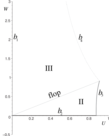
Besides the flop line, this diagram displays additional boundaries labeled “$b_{1}$”, “$b_{2}$”, “$b_{3}$” and “$b_{4}$”, which have the following meaning:

  • The boundary $b_{1}$ corresponds to $\tilde{h}^{0}\rightarrow 0$. The metric on the Kähler cone has an infinite eigenvalue. In the full Kähler cone this limit corresponds to the CY volume becoming zero. However, the vector multiplet manifold of the five-dimensional supergravity theory corresponds to a hypersurface of the Kähler cone, obtained by keeping the total volume constant. In this subspace the singularity takes a different form: while some two-cycles collapse, others diverge, such that the total volume remains at a fixed finite value [9].

  • The boundaries $b_{2}$ and $b_{3}$ correspond to $h^{0}\rightarrow 0$ and $h^{2}\rightarrow 0$, respectively. Here the metric on the Kähler cone degenerates and has a zero eigenvalue. In the microscopic picture a surface is contracted to a point and one obtains tensionless strings. Furthermore, the line $h^{0}\rightarrow 0$ is the fixed volume section of the Kähler cone arising from the elliptic fibration over $\mathbbm{CP}^{2}$. Since one divisor has been blown down, this space has one Kähler modulus less. This boundary component has been called region I in [42].

  • The $b_{4}$ boundary corresponds to $\tilde{h}^{1}\rightarrow 0$. The metric on the Kähler cone is regular. At this boundary one obtains $SU(2)$-enhancement.101010This boundary is one of the models where the corresponding In-picture Lagrangian has been worked out in [17].

We now construct the vector multiplet scalar manifold for the In-picture Lagrangian. The corresponding prepotential is determined by the orbit sum rule (2.33). Taking the average of the prepotentials ${\cal V}_{II}$ and ${\cal V}_{III}$, one finds

$$\begin{split}\hat{\cal V}=&\frac{1}{2}\left({\cal V}_{II}+{\cal V}_{III}\right)\\ =&\frac{7}{24}U^{3}+\frac{1}{2}UT^{2}-\frac{1}{12}W^{3}+\frac{1}{4}U^{2}W-\frac{1}{4}UW^{2}=1\,.\end{split}$$ (2.39)

In order to get the metric $g_{xy}$ on the vector multiplet scalar manifold we take $U$ and $W$ as the vector multiplet scalar fields: $\phi^{x}=U,W$. Solving the constraint for $T$, we obtain

$$T(U,W)=\frac{1}{2}\,\left(\frac{24-7U^{3}+2W^{3}-6U^{2}W+6UW^{2}}{3U}\right)^{1/2}\,.$$ (2.40)

Using the definitions (2.4) and (2.6) it is straightforward to compute the metric $g_{xy}$ in the In-picture,

$$g_{xy}=\left[\begin{array}[]{cc}g_{UU}&g_{WU}\\ g_{WU}&g_{WW}\end{array}\right]\,.$$ (2.41)

Abbreviating

$$K:=24-7U^{3}+2W^{3}-6U^{2}W+6UW^{2}\,,$$ (2.42)

the entries of this matrix are given by

$\displaystyle g_{UU}$ $\displaystyle=$ $\displaystyle\frac{1}{8U^{2}\,K}\,\bigg{(}144-6W^{4}U^{2}+48UW^{2}+4W^{5}U-72U^{2}W\,$
$\displaystyle\qquad\qquad-14U^{3}W^{3}-17U^{4}W^{2}-168U^{3}+24W^{3}+W^{6}\bigg{)}\,,$
$\displaystyle g_{WU}$ $\displaystyle=$ $\displaystyle\frac{1}{8U\,K}\,\bigg{(}24UW-36U^{2}-12W^{2}-W^{5}-4W^{4}U$
$\displaystyle\qquad\qquad+6U^{2}W^{3}+14U^{3}W^{2}+17U^{4}W\bigg{)}\,,$
$\displaystyle g_{WW}$ $\displaystyle=$ $\displaystyle\frac{1}{8\,K}\,\left(48(U+W)+4UW^{3}-6U^{2}W^{2}-14U^{3}W+W^{4}-17U^{4}\right)\,.$

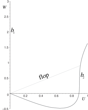
The corresponding vector multiplet scalar manifold is shown in the second diagram of Fig. 1. Besides the flop line at $U=W$ where the metric is regular, this diagram shows two additional boundaries, labeled “$b_{1}$” and “$b_{2}$”. These have the following meaning:

  • The boundary $b_{1}$ corresponds to $U\rightarrow 0$. Here the metric (2.41) has an infinite eigenvalue.

  • At the boundary $b_{2}$ the metric $g_{xy}$ degenerates and has a zero eigenvalue.

Comparing the two diagrams shown in Fig. 1, we find that the boundaries of the vector multiplet scalar manifolds in the Out- and the In-picture are not precisely the same. As explained above, the In-picture LEEA can only be expected to capture the low energy dynamics of M-theory in the vicinity of the flop line $U=W$. In particular, the dynamics near the other boundaries of the Kähler cone is dominated by other states which become light. Therefore it is not clear how to interpret the behavior of the In-picture LEEA far away from the flop line and especially at the boundaries in terms of M-theory physics. Nevertheless, the scalar manifold characterized by (2.41) and depicted in Fig. 1 defines a consistent supergravity action which can be studied in its own right.

3 The hypermultiplet target manifolds

Let us now come to our main issue, the construction of a family of hypermultiplet target manifolds, which can be used to describe the transition states occurring in a flop transition. In this course we will not attempt to derive these manifolds directly from M-theory, but use the Wolf spaces (1.1). In order to find the explicit LEEA we need to know the metrics, the Killing vectors, and the moment maps of these spaces explicitly. As already mentioned, the Wolf spaces also happen to be Kähler, so that one can derive the metric and the Killing vectors from the corresponding Kähler potential. However, the structure relevant for the gauging of isometries is the quaternionic structure, as the scalar potential depends on the moment maps of the Killing vectors, which form a triplet under the $SU(2)$ related to the quaternionic structure. Therefore we will construct these objects from the corresponding quantities on the associated hyper-Kähler cone using the superconformal quotient construction [31, 32, 33]. This method can be applied to any quaternion-Kähler space.

The construction of the Wolf spaces (1.1) has been described in [31] but explicit formulae for the metric have only been given for $X(1)$. The general form of the Killing vectors of $X(N+1)$ has been obtained in [32]. In this section we will derive explicit formulae for the metrics, Killing vectors, and moment maps of all these spaces, while in the next sections we demonstrate that the resulting parametrization is extremely useful for including the transition states in the LEEA.

Before considering the particular family (1.1) of quaternion-Kähler spaces, let us briefly explain the underlying method. From the physical point of view the basic idea is to construct theories with Poincaré supersymmetry as gauge-fixed versions of superconformal theories. In the case at hand one starts with a theory of $n=N+2$ hypermultiplets111111For notational convenience we have set $N+1=n-1$. invariant under rigid superconformal transformations. The corresponding hypermultiplet manifold ${\cal M}_{\mbox{\scriptsize HM}}^{\mbox{\scriptsize SC}}$ is a hyper-Kähler cone, i.e., it is hyper-Kähler and, in addition, possesses a homothetic Killing vector $\chi^{a}$ satisfying $D_{a}\chi^{b}=\delta_{a}^{~{}b}$. This implies that the hyper-Kähler metric $g_{ab}$ of ${\cal M}_{\mbox{\scriptsize HM}}^{\mbox{\scriptsize SC}}$ has a hyper-Kähler potential $\chi$, with $\chi_{a}=D_{a}\chi$ and $g_{ab}=D_{a}D_{b}\chi$. Moreover, ${\cal M}_{\mbox{\scriptsize HM}}^{\mbox{\scriptsize SC}}$ is a cone over a so-called tri-Sasakian manifold with radial coordinate $r=\sqrt{2\chi}$. Superconformal invariance also implies that by multiplying the homothety $\chi^{a}$ with the $SU(2)$ triplet of complex structures $\vec{J}=\left[J^{+},J^{-},J^{3}\right]$ of ${\cal M}_{\mbox{\scriptsize HM}}^{\mbox{\scriptsize SC}}$ one obtains an $SU(2)$ triplet of Killing vectors,

$$\vec{k}^{a}=\vec{J}^{a}_{~{}b}\chi^{b}\,.$$ (3.1)

Using the superconformal calculus, the rigid superconformal theory can be coupled to conformal supergravity and thus be promoted to a locally superconformal theory. This theory is gauge-equivalent to a theory of $n-1$ hypermultiplets coupled to Poincaré supergravity. In this reinterpretation one of the hypermultiplets becomes dependent on the other fields and acts as a compensator. Geometrically this gauging corresponds to performing a superconformal quotient of ${\cal M}_{\mbox{\scriptsize HM}}^{\mbox{\scriptsize SC}}$ with respect to the four conformal Killing vector fields $\chi^{a},\vec{k}^{a}$. The resulting hypermultiplet manifold ${\cal M}_{\mbox{\scriptsize HM}}$ of the Poincaré supergravity theory is quaternion-Kähler. In fact every quaternion-Kähler manifold can be obtained by this construction from its associated hyper-Kähler cone [30].

The construction of the Wolf spaces $X(n-1)$ which have dimension $\dim_{\mathbbm{R}}(X(n-1))=4(n-1)$ proceeds in several steps. First one needs to obtain the hyper-Kähler cone $\mathcal{H}^{(2n)}$ associated with the space $X(n-1)$. In [31] this cone has been constructed as the hyper-Kähler quotient [43] of flat $\mathbbm{C}^{(2n+2)}$ with respect to a particular tri-holomorphic $U(1)$ isometry. Then the superconformal quotient is taken in two steps. First one quotients $\mathcal{H}^{(2n)}$ by the homothetic Killing vector $\chi^{a}$ and the Killing vector $k^{3}=[k^{3a}]$ corresponding to the Cartan direction of the $SU(2)$ isometry group. This quotient is a standard Kähler quotient [44]. The resulting space is the twistor space $\mathcal{Z}^{(2n-2)}$ over $X(n-1)$. In the second step one quotients $\mathcal{Z}^{(2n-2)}$ by the remaining Killing vectors $k^{+}$ and $k^{-}$. The isometry (3.1), however, is only holomorphic and not tri-holomorphic. This implies that at the level of the twistor space, $k^{+}$ and $k^{-}$ are isometries up to $SU(2)$ rotations. In order to obtain well defined quantities on the quaternion-Kähler manifold one has to include a compensating $SU(2)$ transformation. For convenience we have summarized all spaces appearing in this construction in Table 1.

symbol space $\dim_{\mathbbm{R}}$ coordinates
$\mathbbm{C}^{(2n+2)}$ flat complex space $4n+4$ $\left\{z_{+}^{I},\bar{z}_{+}^{I},z_{-I},\bar{z}_{-I}\right\}$
$\mathcal{H}^{(2n)}$ HKC over $X(n-1)$ $4n$ $\left\{z_{+}^{\prime~{}a},\bar{z}_{+}^{\prime~{}a},z_{-a}^{\prime},\bar{z}_{-a}^{\prime}\right\}$
$\mathcal{Z}^{(2n-1)}$ twistor space $4n-2$ $\left\{v^{i},\bar{v}^{i},u_{i},\bar{u}_{i},\zeta,\bar{\zeta}\right\}$
$X(n-1)$ Wolf space $4n-4$ $\left\{v^{i},\bar{v}^{i},u_{i},\bar{u}_{i}\right\}$
Table 1: Summary of the spaces appearing in the quotient construction of the unitary Wolf spaces $X(n-1)$. The index ranges are given by $I=1,\ldots,n+1$ , $a=1,\ldots,n$ and $i=1,\ldots,n-1$.

The rest of this section is organized as follows. In subsection 3.1 we start with flat $\mathbbm{C}^{(2n+2)}$ and construct the metric on $X(n-1)$. The result is given in eqs. (3.45) and (3.1). In subsection 3.2 we construct the Killing vectors of this metric and their tri-holomorphic moment maps. These are given in eq. (3.2) and (3.2), respectively. In subsection 3.3 we use these general results to explicitly construct the Cartan subgroup of the isometry group of $X(2)$. This is needed to construct the gauged LEEA for the model introduced in subsection 2.3. In subsection 3.4 we establish the relation between the quantities constructed in this section and the conventions of the gauged supergravity Lagrangian (2.1). A reader not interested in the technical details of this section may adopt the main results and directly proceed to section 4.

3.1 The metrics of the Wolf spaces $X(n-1)$

The starting point: flat complex space $\mathbbm{C}^{(2n+2)}$

We start our construction by considering $\mathbbm{C}^{(2n+2)}$ with complex coordinates $z^{I}_{+},z_{-I}$, where $I=1,\ldots,n+1$. The metric is taken to be Kähler with the Kähler potential

$$\chi_{(2n+2)}:=\eta_{I\bar{J}}\,z_{+}^{I}\,\bar{z}_{+}^{\bar{J}}+\eta^{I\bar{J}}\,z_{-I}\,\bar{z}_{-\bar{J}}\,.$$ (3.2)

Here $\eta_{I\bar{J}}=\mbox{diag}\left[-,\ldots,-,+,+\right]$ has indefinite signature $(p,q)$ with $p=n-1$ negative and $q=2$ positive eigenvalues, and $\eta^{I\bar{J}}$ is its inverse. This signature of $\eta$ ensures that the space obtained from the quotient construction is of non-compact type, as required by supergravity. Later on the coordinates associated with the negative eigenvalues of $\eta$ will play the role of the hypermultiplet scalars, while the coordinates with the positive eigenvalues act as gauge compensators.

We now promote $\mathbbm{C}^{(2n+2)}$ to a hyper-Kähler manifold. For this purpose we introduce the coordinates $x^{\tilde{I}}:=\left\{z_{+}^{I},\bar{z}_{+}^{\bar{I}},z_{-I},\bar{z}_{-\bar{I}}\right\}$, with $\tilde{I}=1,\ldots,4n+4$. With respect to these coordinates, the $SU(2)$ triplet of complex structures is taken to be:

$\displaystyle J^{1\tilde{I}}_{~{}~{}\tilde{J}}$ $\displaystyle=$ $\displaystyle\left[\begin{array}[]{cccc}0&0&0&{\mathbbm{1}}\\ 0&0&{\mathbbm{1}}&0\\ 0&-{\mathbbm{1}}&0&0\\ -{\mathbbm{1}}&0&0&0\end{array}\right]\,,\quad J^{2\tilde{I}}_{~{}~{}\tilde{J}}=\left[\begin{array}[]{cccc}0&0&0&i{\mathbbm{1}}\\ 0&0&-i{\mathbbm{1}}&0\\ 0&-i{\mathbbm{1}}&0&0\\ i{\mathbbm{1}}&0&0&0\end{array}\right],$ (3.11)
$\displaystyle J^{3\tilde{I}}_{~{}~{}\tilde{J}}$ $\displaystyle=$ $\displaystyle\left[\begin{array}[]{cccc}i{\mathbbm{1}}&0&0&0\\ 0&-i{\mathbbm{1}}&0&0\\ 0&0&i{\mathbbm{1}}&0\\ 0&0&0&-i{\mathbbm{1}}\end{array}\right].$ (3.16)

Here the entries are $(n+1)\times(n+1)$ dimensional block matrices and ${\mathbbm{1}}$ denotes the corresponding unit matrix. These complex structures satisfy the quaternionic algebra $J^{r}J^{s}=-{\mathbbm{1}}\delta^{rs}+\epsilon^{rst}J^{t}$, with $r,s,t=1,2,3$ being the $SU(2)$ index. The complex coordinates $z_{+}^{I},\bar{z}_{+}^{\bar{I}},z_{-I}$ and $\bar{z}_{-\bar{I}}$ are defined with respect to the canonical complex structure $J^{3}$. The Kähler metric $g_{\tilde{I}\tilde{J}}$ derived from (3.2) is hermitian with respect to all three complex structures, $g(J^{r}\,\cdot,J^{r}\,\cdot)=g(\cdot\,,\,\cdot)$.

Instead of working with the basis (3.11), it is more convenient to use $J^{\pm}:=\frac{1}{2}\left(J^{1}\pm iJ^{2}\right)$, since quantities defined with respect to this basis will turn out to be (anti-)holomorphic with respect to $J^{3}$. From these complex structures we obtain the following $SU(2)$ triplet of Kähler forms:

$\displaystyle\omega^{3}$ $\displaystyle=$ $\displaystyle-i\,\eta_{I\bar{J}}\,\mbox{\rm{d}}z_{+}^{I}\,\wedge\,\mbox{\rm{d}}\bar{z}_{+}^{\bar{J}}-i\,\eta^{I\bar{J}}\,\mbox{\rm{d}}z_{-I}\,\wedge\,\mbox{\rm{d}}\bar{z}_{-\bar{J}}\,,$
$\displaystyle\omega^{+}$ $\displaystyle=$ $\displaystyle\mbox{\rm{d}}z_{+}^{I}\,\wedge\,\mbox{\rm{d}}z_{-I}\,,\qquad\omega^{-}=\bar{\omega}^{+}\,.$ (3.17)

Their components are given by

$$\Omega^{3}_{\tilde{I}\tilde{J}}=g_{\tilde{I}\tilde{K}}\,J^{3\tilde{K}}_{~{}~{}~{}\tilde{J}}\,,\quad\Omega^{+}_{\tilde{I}\tilde{J}}=g_{\tilde{I}\tilde{K}}\,J^{+\tilde{K}}_{~{}~{}~{}\tilde{J}}\quad\mbox{and}\quad\Omega^{-}_{\tilde{I}\tilde{K}}=\bar{\Omega}^{+}_{\tilde{I}\tilde{K}}\,,$$ (3.18)

respectively. Here the “bar” denotes complex conjugation with respect to $J^{3}$.

Let us now consider the linear action of the $U(n-1,2)$ isometry subgroup:

$$z^{I}_{+}\rightarrow U^{I}_{~{}J}\,z^{J}_{+}\,,\qquad z_{-I}\rightarrow\left(U^{-1}\right)^{J}_{~{}I}\,z_{-J}\,.$$ (3.19)

With respect to this isometry, the $z_{+}^{I}$ coordinates transform in the fundamental representation of $U(n-1,2)$, while the $z_{-I}$ transform in the complex conjugate representation. Using $\bar{U}^{\bar{I}}_{~{}\bar{J}}=\eta^{\bar{I}K}\left(U^{-1}\right)^{N}_{~{}K}\,\eta_{N\bar{J}}$ one finds that the Kähler potential (3.2) is invariant under this transformation. In principle the isometry group of (3.2) contains additional generators. But since these do not descend to tri-holomorphic isometries of the hyper-Kähler cone $\mathcal{H}^{(2n)}$ they do not give rise to isometries of $X(n-1)$,121212The coset formulation of $X(n-1)$ indicates that the full isometry group of $X(n-1)$ is given by $SU(n-1,2)$. In our approach this $SU(n-1,2)$ arises from the $U(n-1,2)$ above modulo the $U(1)$ gauged in the hyper-Kähler quotient. and will not be considered here.131313The fact that only tri-holomorphic isometries give rise to isometries of the quaternion-Kähler space has been observed in [31].

The Killing vectors of the linearized isometries are given by

$$k_{+\alpha}^{I}=i\,t^{~{}I}_{\alpha~{}J}\,z_{+}^{J}\,,\qquad k_{-\alpha I}=-i\,t^{~{}J}_{\alpha~{}I}\,z_{-J}\,.$$ (3.20)

Here $\alpha$ numerates the $n(n+2)+1$ generators of $U(n-1,2)$, $t^{~{}I}_{\alpha~{}J}$. To simplify our notation we will drop the index $\alpha$ in the following. The action of these Killing vectors is tri-holomorphic, i.e., the Lie derivative with respect to $k$ satisfies $\mathcal{L}_{k}J^{r}=0$ for all three complex structures (3.11). This implies in particular that the Killing vectors are holomorphic with respect to $J^{3}$. Hence we can obtain their components with respect to $\bar{z}_{+}^{\bar{I}}$ and $\bar{z}_{-\bar{I}}$ by complex conjugation of $k^{I}_{+}$ and $k_{-I}$, respectively.

The condition that the vectors $k$ are Killing, $\mathcal{L}_{k}g=0$, as well as tri-holomorphic implies that they are Hamiltonian, $\mathcal{L}_{k}\omega^{r}=0$. The last statement provides the integrability condition for the moment maps associated with these isometries. They are obtained as the solution of the equation

$$\frac{\partial\mu^{r}}{\partial x^{\tilde{I}}}:=\Omega^{r}_{\tilde{I}\tilde{J}}\,k^{\tilde{J}}\,,$$ (3.21)

where $r=+,-,3$. Substituting the Killing vectors (3.20) and the Kähler forms (3.18), these equations are easily integrated and yield:

$\displaystyle\mu^{3}$ $\displaystyle=$ $\displaystyle-\bar{z}^{\bar{J}}_{+}\,\eta_{\bar{J}I}\,t^{I}_{~{}K}\,z^{K}_{+}\,+\,z_{-I}\,t^{I}_{~{}J}\,\eta^{J\bar{K}}\,\bar{z}_{-\bar{K}}\,,$
$\displaystyle\mu^{+}$ $\displaystyle=$ $\displaystyle-i\,z_{-I}\,t^{I}_{~{}J}\,z^{J}_{+}\,,\qquad\,\mu^{-}=\bar{\mu}^{+}\,.$ (3.22)

Here we omitted the constants of integration, which, in principle, could give rise to Fayet-Iliopoulous terms. Since these terms appear in neither the superconformal theory defined on the level of the hyper-Kähler cone nor in the $D=5$ supergravity action reviewed in subsection 2.1, the moment maps (3.1) will give rise to the most general moment maps compatible with the action (2.1).

The hyper-Kähler quotient construction of $\mathcal{H}^{(2n)}$

We now perform the hyper-Kähler quotient construction of $\mathcal{H}^{(2n)}$ by taking the quotient of $\mathbbm{C}^{(2n+2)}$ with respect to the $U(1)$ isometry which acts on $z_{+}^{I}$ and $z_{-I}$ by opposite phase transformations. The infinitesimal generator of this isometry is given by $t^{I}_{~{}J}=\delta^{I}_{~{}J}$. Substituting this generator into (3.1) we find:

$$\mu^{3}=-\eta_{I\bar{J}}\,z^{I}_{+}\,\bar{z}^{\bar{J}}_{+}\,+\,\eta^{I\bar{J}}\,z_{-I}\,\bar{z}_{-\bar{J}}\,,\quad\mu^{+}=-i\,z^{I}_{+}\,z_{-I}\,,\quad\mu^{-}=\bar{\mu}^{+}\,.$$ (3.23)

The quotient is performed by first introducing $U(1)$ invariant coordinates $z^{\prime~{}I}_{+}$, $z^{\prime}_{-~{}I}$ on $\mathbbm{C}^{(2n+2)}$ and substituting these into the moment maps (3.23). We then set the resulting moment maps to zero and solve these constraints in terms of $z^{\prime~{}n+1}_{+}$, $z_{-n+1}^{\prime}$ and their complex conjugates. The remaining unconstrained coordinates $z^{\prime~{}a}_{+}$, $z_{-a}^{\prime}$ with $a=1,\ldots,n$ provide coordinates on $\mathcal{H}^{(2n)}$. In practice, we choose the primed coordinates as

$$z^{\prime I}_{+}:=\frac{z^{I}_{+}}{z^{n+1}_{+}},\qquad\qquad z^{\prime}_{-I}:=z_{-I}\,z_{+}^{n+1}\,.$$ (3.24)

In terms of these coordinates the moment maps (3.23) become

$\displaystyle\mu^{3}$ $\displaystyle=$ $\displaystyle-\eta_{I\bar{J}}\,z^{\prime I}_{+}\,\bar{z}^{\prime\bar{J}}_{+}\,\left(\bar{z}^{n+1}_{+}\,z^{n+1}_{+}\right)+\,\eta^{I\bar{J}}\,z_{-I}^{\prime}\,\bar{z}_{-\bar{J}}^{\prime}\,\left(\bar{z}^{n+1}_{+}\,z^{n+1}_{+}\right)^{-1}\,,$
$\displaystyle\mu^{+}$ $\displaystyle=$ $\displaystyle-i\,z^{\prime I}_{+}\,z_{-I}^{\prime}\,,\,\qquad\,\mu^{-}=\bar{\mu}^{+}\,.$ (3.25)

Setting the moment maps to zero and solving the resulting constraints in terms of $z^{\prime~{}n+1}_{+}$, $z_{-n+1}^{\prime}$ and their complex conjugates yields

$$\left(\bar{z}^{n+1}_{+}\,z^{n+1}_{+}\right)=\left(\frac{\eta^{I\bar{J}}\,z_{-I}^{\prime}\,\bar{z}_{-\bar{J}}^{\prime}}{\eta_{I\bar{J}}\,z^{\prime I}_{+}\,\bar{z}^{\prime\bar{J}}_{+}}\right)^{1/2}\,,\quad z^{\prime~{}n+1}_{+}=1\,,\quad z^{\prime}_{-n+1}=-\,z^{\prime~{}a}_{+}\,z^{\prime}_{-a}\,.$$ (3.26)

Substituting the new coordinates (3.24) into the Kähler potential (3.2) and performing the gauge fixing gives the Kähler potential for the metric on $\mathcal{H}^{(2n)}$:

$$\chi_{\mathcal{H}}(z^{a}_{+},\bar{z}_{+}^{a},z_{-a},z_{-a})=2\,\chi_{+}\,\chi_{-}\,.$$ (3.27)

Here we introduced

$$\chi_{+}:=\left(\eta_{I\bar{J}}\,z^{\prime~{}I}_{+}\,\bar{z}^{\prime~{}\bar{J}}_{+}\right)^{1/2}\,,\qquad\,\chi_{-}:=\left(\eta^{I\bar{J}}\,z_{-I}^{\prime}\,\bar{z}_{-\bar{J}}^{\prime}\right)^{1/2}\,,$$ (3.28)

where it is understood that we have performed the gauge fixing (3.26).

In view of the later steps in the construction we also calculate $\omega^{+}_{\mathcal{H}}$. Substituting the primed coordinates into (3.1) and performing the gauge fixing gives

$$\omega^{+}_{\mathcal{H}}=\mbox{\rm{d}}z^{\prime~{}a}_{+}\,\wedge\,\mbox{\rm{d}}z^{\prime}_{-a}\,.$$ (3.29)

The superconformal quotient: Going to twistor space $\mathcal{Z}^{(2n-1)}$

We now descend to the twistor space $\mathcal{Z}^{(2n-1)}$. Here we follow [31] and introduce the coordinates

$$z^{\prime}_{-i}=\mbox{\rm{e}}^{2z}\,u_{i}\,,\qquad z_{-n}^{\prime}=\mbox{\rm{e}}^{2z}\,,\qquad i=1,\ldots,n-1\,.$$ (3.30)

We next single out another coordinate, $\zeta$, which will be gauged when going to $X(n-1)$. To this end, we substitute the coordinates (3.30) into $\omega^{+}_{\mathcal{H}}$ given in eq. (3.29):

$$\omega^{+}_{\mathcal{Z}}=\mbox{\rm{e}}^{2z}\left(2\,\mbox{\rm{d}}z^{\prime~{}n}_{+}+2\,u_{i}\,\mbox{\rm{d}}z^{\prime~{}i}_{+}\right)\wedge\,\mbox{\rm{d}}z+\mbox{\rm{e}}^{2z}\,\mbox{\rm{d}}z^{\prime~{}i}_{+}\,\wedge\,\mbox{\rm{d}}u_{i}\,.$$ (3.31)

Following the general construction of the superconformal quotient, the components of this 2-form should be compared to

$$\Omega_{\tilde{a}\tilde{b}}^{+}\left(u,z,z^{\prime}_{+}\right)=\mbox{\rm{e}}^{2z}\,\left[\begin{array}[]{cc}\omega_{\tilde{\imath}\tilde{\jmath}}(u,z^{\prime}_{+})&X_{\tilde{\imath}}(u,z^{\prime}_{+})\\ -X_{\tilde{\jmath}}(u,z^{\prime}_{+})&0\end{array}\right]\,.$$ (3.32)

From this comparison, we obtain the explicit form of $X_{\tilde{\imath}}$:

$$X_{\tilde{\imath}}=\left[\underbrace{0\,,\,\ldots\,,\,0}_{(n-1)\mbox{times}},\,2\,u_{1}\,,\,\ldots\,,\,2\,u_{n-1}\,,\,2\,\right]^{\rm T}\,.$$ (3.33)

We then determine $\zeta$ by first finding a $Y^{\tilde{\imath}}$, subject to $X_{{\tilde{\imath}}}Y^{{\tilde{\imath}}}=1$ and independent of the coordinates $z^{\prime~{}a}_{+},u_{i},z$. The coordinate $\zeta$ is obtained as the solution of the differential equation

$$Y^{\tilde{\imath}}\,\frac{\partial}{\partial z^{\tilde{\imath}}}=\frac{\partial}{\partial\zeta}\,.$$ (3.34)

Choosing $Y^{\tilde{\imath}}=\left[0,\ldots,0,1/2\right]$, which is natural but not unique, we find $\zeta=2z^{\prime~{}n}_{+}$. This motivates to introduce

$$z^{\prime~{}i}_{+}=v^{i}\,,\qquad z^{\prime~{}n}_{+}=\frac{1}{2}\,\zeta\,.$$ (3.35)

The $v^{i},u_{i},\zeta$ and their complex conjugates then provide coordinates on the twistor space $\mathcal{Z}^{(2n-1)}$. In order to obtain the Kähler potential of $\mathcal{Z}^{(2n-1)}$ we first substitute these new coordinates into $\chi_{+}$ and $\chi_{-}$:

$\displaystyle\chi_{+}$ $\displaystyle=$ $\displaystyle\left(1+\eta_{i\bar{\jmath}}\,v^{i}\bar{v}^{\bar{\jmath}}+\frac{1}{4}\,\zeta\,\bar{\zeta}\right)^{1/2}\,,$
$\displaystyle\chi_{-}$ $\displaystyle=$ $\displaystyle\mbox{\rm{e}}^{z+\bar{z}}\left(1+\eta^{i\bar{\jmath}}\,u_{i}\bar{u}_{\bar{\jmath}}+\left(v^{i}u_{i}+\frac{1}{2}\zeta\right)\left(\bar{v}^{\bar{\imath}}\,\bar{u}_{\bar{\imath}}+\frac{1}{2}\bar{\zeta}\right)\right)^{1/2}\,.$ (3.36)

The Kähler potential of $\mathcal{Z}^{(2n-1)}$, $K(v,u,\zeta,\bar{v},\bar{u},\bar{\zeta})$, can be deduced by comparing $\chi_{\mathcal{H}}$ given in (3.27) to the following expression:

$$\chi_{\mathcal{H}}=\mbox{\rm{e}}^{z+\bar{z}+K(v,u,\zeta,\bar{v},\bar{u},\bar{\zeta})}\,.$$ (3.37)

From this we read off

$$K(v,u,\zeta,\bar{v},\bar{u},\bar{\zeta})=\ln\left(\chi_{+}\right)+\ln\left(\chi_{-}\right)+\ln\left(2\right)\,,$$ (3.38)

where $\chi_{+}$ and $\chi_{-}$ are taken at $z=0$.

In order to calculate the $SU(2)$ compensators appearing in the construction of the metric of $X(n-1)$, we also need $\omega_{\mathcal{Z}}^{+}$ in terms of the coordinates $v^{i},u_{i},z,\zeta$. By substituting these coordinates into (3.31) we obtain

$$\omega^{+}_{\mathcal{Z}}=\mbox{\rm{e}}^{2z}\left(\mbox{\rm{d}}\zeta+2\,u_{i}\,\mbox{\rm{d}}v^{i}\right)\wedge\mbox{\rm{d}}z+\mbox{\rm{e}}^{2z}\,\mbox{\rm{d}}v^{i}\,\wedge\,\mbox{\rm{d}}u_{i}\,.$$ (3.39)

The superconformal quotient: The metric on $X(n-1)$

We now descend to the quaternion-Kähler space $X(n-1)$ by setting $\zeta=0$. The Kähler potential $K$ becomes

$$K(u,v,0,\bar{u},\bar{v},0)=\frac{1}{2}\,\ln\left(\phi_{+}\right)+\frac{1}{2}\,\ln\left(\phi_{-}\right)+\ln\left(2\right)\,,$$ (3.40)

where we introduced

$$\phi_{+}:=1+\eta_{i\bar{\jmath}}\,v^{i}\bar{v}^{\bar{\jmath}}\,,\quad\phi_{-}:=1+\eta^{i\bar{\jmath}}\,u_{i}\bar{u}_{\bar{\jmath}}+\left(v^{i}u_{i}\right)\left(\bar{v}^{\bar{\imath}}\,\bar{u}_{\bar{\imath}}\right)\,.$$ (3.41)

However, since $\zeta$ is not parallel to the Killing vector $k^{+}$ given in (3.1), the condition $\zeta=0$ is not preserved. In order to obtain the metric $G_{\alpha\bar{\beta}}$ on $X(n-1)$ we need to include an additional compensating transformation. Explicitly we have

$$G_{\alpha\bar{\beta}}=K_{\alpha\bar{\beta}}-\mbox{\rm{e}}^{-2K}\,X_{\alpha}\,\bar{X}_{\bar{\beta}}\,,$$ (3.42)

where $K_{\alpha\bar{\beta}}$ is the Kähler metric obtained from (3.40) and $\alpha=1,\ldots,2n-2$ enumerates the coordinates $\{v^{1},\ldots,v^{n-1},u_{1},\ldots,u_{n-1}\}$. In order to determine the explicit from of the $X_{\alpha}$ appearing in the compensating transformation, we compare the components of $\omega^{+}_{\mathcal{Z}}$ given in (3.39) to the general form of $\omega^{+}_{\mathcal{Z}}$ given in [31]:

$$\Omega^{+}_{ab}=\mbox{\rm{e}}^{2z}\left[\begin{array}[]{ccc}\omega_{\alpha\beta}(v,u)&0&X_{\alpha}(v,u)\\ 0&0&1\\ -X_{\beta}(v,u)&-1&0\end{array}\right]\,.$$ (3.43)

From this we read off

$$X_{\alpha}=\left[\,2\,u_{1}\,,\,\ldots\,,\,2\,u_{n-1}\,,\underbrace{\,0\,,\,\ldots\,,0\,}_{(n-1)\mbox{ times}}\right]^{\rm T}\,.$$ (3.44)

Having all these ingredients at hand, we can now write down the metric (3.42) explicitly. Arranging our indices as $X,Y=\left\{v^{i},\bar{v}^{\bar{\imath}},u_{i},\bar{u}_{\bar{\imath}}\right\}$ the components of $G_{\alpha\bar{\beta}}$ can be read off from the following matrix:

$$G_{XY}=\left[\begin{array}[]{cccc}0&G_{v\bar{v}}&0&G_{v\bar{u}}\\ G_{\bar{v}v}&0&G_{\bar{v}u}&0\\ 0&G_{u\bar{v}}&0&G_{u\bar{u}}\\ G_{\bar{u}v}&0&G_{\bar{u}u}&0\\ \end{array}\right]\,.$$ (3.45)

The entries of this matrix are given by

$\displaystyle G_{u_{i}\bar{u}_{\bar{\jmath}}}$ $\displaystyle=$ $\displaystyle\frac{1}{2\phi_{-}}\left(\eta^{i\bar{\jmath}}+\bar{v}^{\bar{\jmath}}\,v^{i}\right)-\frac{1}{2\phi_{-}^{2}}\left(\eta^{\bar{\jmath}l}u_{l}+\bar{v}^{\bar{\jmath}}\left(v^{l}u_{l}\right)\right)\big{(}\eta^{i\bar{l}}\bar{u}_{\bar{l}}+v^{i}\big{(}\bar{v}^{\bar{l}}\bar{u}_{\bar{l}}\big{)}\big{)}\,,$
$\displaystyle G_{\bar{v}^{\bar{\imath}}u_{j}}$ $\displaystyle=$ $\displaystyle\frac{1}{2\phi_{-}^{2}}\,\left(\bar{u}_{\bar{\imath}}v^{j}\,\left(1+\eta^{k\bar{l}}u_{k}\bar{u}_{\bar{l}}\right)-\bar{u}_{\bar{\imath}}\eta^{j\bar{l}}\bar{u}_{\bar{l}}\left(v^{l}u_{l}\right)\right)\,,$ (3.46)
$\displaystyle G_{v^{i}\bar{v}^{\bar{\jmath}}}$ $\displaystyle=$ $\displaystyle\frac{1}{2\phi_{+}}\,\eta_{i\bar{\jmath}}-\frac{1}{2\phi_{+}^{2}}\,\big{(}\eta_{i\bar{l}}\,\bar{v}^{\bar{l}}\big{)}\,\big{(}\eta_{\bar{\jmath}l}\,v^{l}\big{)}\,-\,\frac{1}{\phi_{+}\phi_{-}}\,u_{i}\bar{u}_{\bar{\jmath}}$
$\displaystyle+\,\frac{1}{2\phi_{-}}\,u_{i}\,\bar{u}_{\bar{\jmath}}\,-\,\frac{1}{2\phi_{-}^{2}}\,u_{i}\,\bar{u}_{\bar{\jmath}}\,\big{(}v^{l}\,u_{l}\big{)}\big{(}\bar{v}^{\bar{l}}\bar{u}_{\bar{l}}\big{)}\,.$

The other non-vanishing entries of the matrix can be obtained from the relations $G_{v^{i}\bar{v}^{\bar{\jmath}}}=G_{\bar{v}^{\bar{\jmath}}v^{i}}$, $G_{u_{i}\bar{u}_{\bar{\jmath}}}=G_{\bar{u}_{\bar{\jmath}}u_{i}}$, $G_{v^{i}\bar{u}_{\bar{\jmath}}}=G_{\bar{u}_{\bar{\jmath}}v^{i}}$ and $G_{v^{i}\bar{u}_{\bar{\jmath}}}=\left(G_{\bar{v}^{\bar{\imath}}u_{j}}\right)^{*}$, where “” denotes complex conjugation.

These results provide metrics of $X(n-1)$, which obviously are hermitian but not Kähler with respect to $J^{3}$. In fact the holomorphic assignments in (3.1) are adapted to the quaternionic structure, which cannot be used to define a Kähler potential. However, there must be a non-holomorphic coordinate transformation which brings the metric given above into its standard Kähler form [28].

To conclude this subsection, let us comment on the special case $n=2$, which corresponds to the universal hypermultiplet. In this case the index $i$ has only a single value and may be omitted. Setting $\eta_{i\bar{\jmath}}=\eta_{1\bar{1}}=-1$ the general metric (3.1) simplifies to

$\displaystyle G_{u\bar{u}}$ $\displaystyle=$ $\displaystyle-\,\frac{1}{2\phi_{-}^{2}}\,\left(1-v\bar{v}\right)\,,$
$\displaystyle G_{u\bar{v}}$ $\displaystyle=$ $\displaystyle\frac{1}{2\phi_{-}^{2}}\,\bar{u}v\,,$ (3.47)
$\displaystyle G_{v\bar{v}}$ $\displaystyle=$ $\displaystyle-\,\frac{1}{2\,\phi_{+}^{2}\,\phi_{-}^{2}}\,\left(1-u\bar{u}\left(1-v\bar{v}\right)^{2}\right)\,.$

This is exactly the metric for the universal hypermultiplet derived in [31].

3.2 The isometries of the Wolf spaces $X(n-1)$

After obtaining the metric on $X(n-1)$, we will now derive the second ingredient needed in the construction of the LEEA and derive the Killing vectors and moment maps of the unitary Wolf spaces. We follow the calculation of [32] and extend these results.

The Killing vectors of flat $\mathbbm{C}^{(2n+2)}$ are given in (3.20). In order to find the Killing vectors on the hyper-Kähler cone $\mathcal{H}^{(2n)}$ we perform a coordinate transformation to the primed coordinates (3.24). The resulting Killing vectors read:

$$k^{\prime a}_{+}=i\,t^{a}_{~{}I}\,z^{\prime I}_{+}-\,i\,z^{\prime a}_{+}\,t^{n+1}_{~{}~{}I}\,z^{\prime I}_{+}\,,\quad k^{\prime}_{-a}=\,i\,z_{-a}^{\prime}\,t^{n+1}_{~{}~{}~{}I}\,z^{\prime~{}I}_{+}-\,i\,t^{I}_{~{}a}\,z^{\prime}_{-I}\,.$$ (3.48)

Here we have implicitly performed the gauge fixing (3.26).

To obtain the Killing vectors on $X(n-1)$ we first transform (3.48) into the coordinates $v^{i},u_{i},z,\zeta$ given by

$$z^{\prime~{}i}_{+}=v^{i}\,,\qquad z^{\prime~{}n}_{+}=\frac{1}{2}\,\zeta\,,\qquad z_{-i}^{\prime}=\mbox{\rm{e}}^{2z}\,u_{i}\,,\qquad z_{-n}^{\prime}=\mbox{\rm{e}}^{2z}\,.$$ (3.49)

Fixing $\zeta=0$, the resulting vectors $k^{\alpha}$ read:

$$\begin{split}k^{v^{i}}&=\,i\,t^{i}_{~{}j}\,v^{j}+i\,t^{i}_{~{}n+1}-i\,v^{i}\,t^{n+1}_{~{}~{}~{}j}\,v^{j}-i\,v^{i}\,t^{n+1}_{~{}~{}~{}n+1}\,,\\ k^{\zeta}&=2\,i\,\left(t^{n}_{~{}i}\,v^{i}+t^{n}_{~{}n+1}\right)\,,\\ k_{z}&=\frac{i}{2}\left(t^{n+1}_{~{}~{}~{}i}v^{i}+t^{n+1}_{~{}~{}~{}n+1}-t^{i}_{~{}n}\,u_{i}-t^{n}_{~{}n}+t^{n+1}_{~{}~{}~{}n}\,v^{i}\,u_{i}\right)\,,\\ k_{u_{i}}&=i\,u_{i}\,\left(t^{n+1}_{~{}~{}~{}j}\,v^{j}+t^{n+1}_{~{}~{}~{}n+1}\right)-i\,t^{j}_{~{}i}u_{j}-i\,t^{n}_{~{}i}+i\,t^{n+1}_{~{}~{}~{}i}\,\left(v^{j}\,u_{j}\right)-2\,u_{i}\,k_{z}\,.\end{split}$$ (3.50)

However, these vectors do not preserve the gauge $\zeta=0$. In order to get the Killing vectors $\hat{k}^{\alpha}$ on $X(n-1)$ we have to implement an additional compensating transformation, which is given by [32]:

$$\hat{k}^{\alpha}=k^{\alpha}-\,\frac{X^{\alpha}}{X^{\zeta}}\,k^{\zeta}\,.$$ (3.51)

According to [31], $X^{\alpha},X^{\zeta}$ can be determined from the equations

$$X^{\alpha}=\left(\hat{\omega}^{\alpha\beta}K_{\beta}+Z^{\alpha}\,K_{\zeta}\right)\,\mbox{\rm{e}}^{2K}\,,\quad X^{\zeta}=\left(1-Z^{\alpha}K_{\alpha}\right)\mbox{\rm{e}}^{2K}\,,$$ (3.52)

with $\hat{\omega}^{\alpha\beta}$ and $Z^{\alpha}$ given by

$$\hat{\omega}^{\alpha\gamma}\omega_{\gamma\beta}=-\delta^{\alpha}_{~{}\beta}\,,\qquad Z^{\alpha}=-\,\hat{\omega}^{\alpha\beta}\,X_{\beta}\,.$$ (3.53)

Here $K$ is the Kähler potential (3.38), $K_{\alpha}$ and $K_{\zeta}$ denote its derivative with respect to $v^{i},u_{i}$ and $\zeta$, respectively, and $X_{\alpha}$ is given in (3.44). The $\omega_{\alpha\beta}$ is determined by comparing $\omega^{+}_{\mathcal{Z}}$ given in (3.39) with the general expression (3.43) and $\hat{\omega}^{\alpha\beta}$ is obtained from eq. (3.53). Explicitly, we find

$$\omega_{\alpha\beta}=\left[\begin{array}[]{cc}0&{\mathbbm{1}}\\ -{\mathbbm{1}}&0\end{array}\right]\,,\qquad\hat{\omega}^{\alpha\beta}=\left[\begin{array}[]{cc}0&{\mathbbm{1}}\\ -{\mathbbm{1}}&0\end{array}\right]\,,$$ (3.54)

where ${\mathbbm{1}}$ denotes the $n-1$-dimensional unit matrix. Substituting $X_{\alpha}$ into (3.53) gives

$$Z^{\alpha}=\left[\underbrace{\,0\,,\ldots,\,0}_{n-1\,\mbox{times}}\,,\,2\,u_{1}\,,\,\ldots\,,\,2\,u_{n-1}\right]^{\rm T}\,.$$ (3.55)

With these results at hand, it is now straightforward to write down the explicit form of the compensating transformation appearing in (3.51):

$$\frac{X^{v^{i}}}{X^{\zeta}}=\frac{1}{2}\left(\eta^{i\bar{\jmath}}\,\bar{u}_{\bar{\jmath}}+v^{i}\left(\bar{v}^{\bar{\jmath}}\bar{u}_{\bar{\jmath}}\right)\right)\,,\qquad\frac{X^{u_{i}}}{X^{\zeta}}=\,-\,\frac{\phi_{-}}{2\phi_{+}}\,\eta_{i\bar{\jmath}}\,\bar{v}^{\bar{\jmath}}\,.$$ (3.56)

The Killing vectors of $X(n-1)$ then read:

$\displaystyle\hat{k}^{v^{i}}$ $\displaystyle=$ $\displaystyle i\,t^{i}_{~{}j}\,v^{j}+i\,t^{i}_{~{}n+1}-i\,v^{i}\,t^{n+1}_{~{}~{}~{}j}\,v^{j}-i\,v^{i}\,t^{n+1}_{~{}~{}~{}n+1}-\,\frac{k^{\zeta}}{2}\left(\eta^{i\bar{\jmath}}\bar{u}_{\bar{\jmath}}+v^{i}\,\bar{v}^{\bar{k}}\bar{u}_{\bar{k}}\right)\,,$
$\displaystyle\hat{k}^{u_{i}}$ $\displaystyle=$ $\displaystyle i\,u_{i}\,\left(t^{n+1}_{~{}~{}~{}j}v^{j}+t^{n+1}_{~{}~{}~{}n+1}\right)-i\,t^{j}_{~{}i}\,u_{j}-i\,t^{n}_{~{}i}+i\,t^{n+1}_{~{}~{}~{}i}\,\left(v^{j}\,u_{j}\right)\,$
$\displaystyle\qquad\qquad-2u_{i}\,k_{z}+\frac{\phi_{-}}{2\phi_{+}}\,k^{\zeta}\,\eta_{i\bar{\jmath}}\,\bar{v}^{\bar{\jmath}}\,.$

Here $k^{\zeta}$ and $k_{z}$ are given in (3.50).

We will now derive the moment maps associated with these Killing vectors, starting from the moment maps on flat $\mathbbm{C}^{(2n+2)}$ given in (3.1). Rewriting them in terms of the primed coordinates, the corresponding moment maps on $\mathcal{H}^{(2n)}$ are:

$$\begin{split}\mu^{3}&=-\,\frac{2}{\chi_{(2n)}}\left(\chi_{-}^{2}\,\bar{z}_{+}^{\prime\bar{I}}\,\eta_{\bar{I}J}t^{J}_{~{}K}\,z^{\prime K}_{+}-\chi_{+}^{2}\,z^{\prime}_{-K}\,t^{K}_{~{}J}\,\eta^{J\bar{I}}\bar{z}^{\prime}_{-\bar{I}}\right)\,,\\ \mu^{+}&=-\,i\,z^{\prime}_{-I}\,t^{I}_{~{}J}\,z^{\prime J}_{+}\,,\qquad\mu^{-}=\bar{\mu}^{+}\,.\end{split}$$ (3.58)

Again, it is understood that these expressions implicitly contain the gauge fixing (3.26).

In [32] it was found that the moment maps on the hyper-Kähler cone, $\mu^{r}$, and the moment maps on the underlying quaternion-Kähler manifold, $\hat{\mu}^{r}$, are related by

$$\mu^{3}=\chi_{(2n)}\,\hat{\mu}^{3}\,,\qquad\mu^{+}=\mbox{\rm{e}}^{z-\bar{z}}\,\chi_{(2n)}\,\hat{\mu}^{+}\,,\qquad\hat{\mu}^{-}=\bar{\hat{\mu}}^{+}\,.$$ (3.59)

Substituting in the coordinate transformation (3.49) and gauging $\zeta=0$, we obtain the following expression for the moment maps on $X(n-1)$:

$\displaystyle\hat{\mu}^{3}$ $\displaystyle=$ $\displaystyle-\,\frac{1}{2\phi_{+}}\left\{\bar{v}^{\bar{\imath}}\,\eta_{\bar{\imath}j}\,t^{j}_{~{}k}\,v^{k}+t^{n+1}_{~{}~{}~{}i}\,v^{i}+\bar{v}^{\bar{\jmath}}\,\eta_{\bar{\jmath}i}\,t^{i}_{~{}n+1}+t^{n+1}_{~{}~{}~{}n+1}\right\}$
$\displaystyle+\frac{1}{2\phi_{-}}\big{\{}u_{i}\,t^{i}_{~{}j}\,\eta^{j\bar{k}}\,\bar{u}_{\bar{k}}+u_{i}\,t^{i}_{~{}n}+t^{n}_{~{}i}\,\eta^{i\bar{\jmath}}\,\bar{u}_{\bar{\jmath}}+t^{n}_{~{}n}-\left(u_{i}\,t^{i}_{~{}n+1}+t^{n}_{~{}n+1}\right)\left(\bar{u}_{\bar{\imath}}\bar{v}^{\bar{\imath}}\right)$
$\displaystyle\qquad\qquad-\left(t^{n+1}_{~{}~{}~{}i}\,\eta^{i\bar{\jmath}}\,\bar{u}_{\bar{\jmath}}+t^{n+1}_{~{}~{}~{}n}\right)\,\left(u_{k}v^{k}\right)+t^{n+1}_{~{}~{}~{}n+1}\,\left(u_{i}\,v^{i}\right)\,\left(\bar{u}_{\bar{\jmath}}\bar{v}^{\bar{\jmath}}\right)\big{\}}\,,$
$\displaystyle\hat{\mu}^{+}$ $\displaystyle=$ $\displaystyle-\,\frac{i}{2\phi_{+}^{1/2}\phi_{-}^{1/2}}\,\big{\{}u_{i}\,t^{i}_{~{}j}\,v^{j}+t^{n}_{~{}j}\,v^{j}-t^{n+1}_{~{}~{}~{}i}\,v^{i}\left(u_{j}\,v^{j}\right)+u_{i}\,t^{i}_{~{}n+1}$
$\displaystyle\qquad\qquad\qquad+t^{n}_{~{}n+1}-t^{n+1}_{~{}~{}~{}n+1}\left(u_{i}\,v^{i}\right)\big{\}}\,.$

This result completes the derivation of the Killing vectors and moment maps of $X(n-1)$. Together with the metric (3.45) we now have all the ingredients for modeling the hypermultiplet sector of our In-picture LEEA.

3.3 Examples of Isometries on $X(2)$

Before we embark upon this construction, we will use our general results (3.2) and (3.2) to explicitly calculate the Killing vectors and moment maps of the Cartan subgroup of the isometry group on $X(2)$, $SU(2,2)$. As it will turn out in the next section, this information already suffices to construct the In-picture Lagrangian for the model introduced in subsection 2.3.

We choose the three Cartan generators of $SU(2,2)$ as

$\displaystyle C_{1}$ $\displaystyle=$ $\displaystyle\frac{1}{2}\,{\rm diag}\left[\,1\,,\,-1\,,\,0\,,0\,\right]\,,$
$\displaystyle C_{2}$ $\displaystyle=$ $\displaystyle\frac{1}{2}\,{\rm diag}\left[\,0\,,\,0\,,\,1\,,-1\,\right]\,,$ (3.61)
$\displaystyle C_{3}$ $\displaystyle=$ $\displaystyle\frac{1}{2\sqrt{2}}\,{\rm diag}\left[\,1\,,\,1\,,\,-1\,,-1\,\right]\,.$

Substituting these matrices into the expression for a generic Killing vector on $X(2)$ (3.2), we find:

$\displaystyle k_{1}$ $\displaystyle=$ $\displaystyle\frac{i}{2}\,\left[v^{1},-v^{2},-\bar{v}^{1},\bar{v}^{2},-u_{1},u_{2},\bar{u}_{1},-\bar{u}_{2}\right]^{\rm T}\,,$
$\displaystyle k_{2}$ $\displaystyle=$ $\displaystyle\frac{i}{2}\,\left[v^{1},v^{2},-\bar{v}^{1},-\bar{v}^{2},u_{1},u_{2},-\bar{u}_{1},-\bar{u}_{2}\right]^{\rm T}\,,$ (3.62)
$\displaystyle k_{3}$ $\displaystyle=$ $\displaystyle\frac{i}{\sqrt{2}}\,\left[v^{1},v^{2},-\bar{v}^{1},-\bar{v}^{2},-u_{1},-u_{2},\bar{u}_{1},\bar{u}_{2}\right]^{\rm T}\,.$

Here the index $\alpha$ in $k_{\alpha}$ enumerates the Cartan generators. The components of the Killing vectors are given with respect to the basis

$$\left\{\partial_{v^{1}},\partial_{v^{2}},\partial_{\bar{v}^{1}},\partial_{\bar{v}^{2}},\partial_{u_{1}},\partial_{u_{2}},\partial_{\bar{u}_{1}},\partial_{\bar{u}_{2}}\right\}\,.$$ (3.63)

When gauging these isometries, we also need the triplet of moment maps corresponding to the Killing vectors. These are obtained by evaluating eq. (3.2) for the generators (3.3). The resulting moment maps are:

$\displaystyle\hat{\mu}_{1}$ $\displaystyle=$ $\displaystyle\left[\begin{array}[]{c}-\frac{i}{4\phi_{+}^{1/2}\phi_{-}^{1/2}}\,\left(v^{1}u_{1}-v^{2}u_{2}-\bar{v}^{1}\bar{u}_{1}+\bar{v}^{2}\bar{u}_{2}\right)\\ -\,\frac{1}{4\phi_{+}^{1/2}\phi_{-}^{1/2}}\,\left(v^{1}u_{1}-v^{2}u_{2}+\bar{v}^{1}\bar{u}_{1}-\bar{v}^{2}\bar{u}_{2}\right)\\ \frac{1}{4\,\phi_{+}}\left(\bar{v}^{1}v^{1}-\bar{v}^{2}v^{2}\right)-\frac{1}{4\,\phi_{-}}\left(\bar{u}_{1}u_{1}-\bar{u}_{2}u_{2}\right)\end{array}\right]\,,$ (3.67)
$\displaystyle\hat{\mu}_{2}$ $\displaystyle=$ $\displaystyle\left[\begin{array}[]{c}-\,\frac{i}{4\phi_{+}^{1/2}\phi_{-}^{1/2}}\,\left(v^{1}u_{1}+v^{2}u_{2}-\bar{v}^{1}\bar{u}_{1}-\bar{v}^{2}\bar{u}_{2}\right)\\ -\,\frac{1}{4\phi_{+}^{1/2}\phi_{-}^{1/2}}\,\left(v^{1}u_{1}+v^{2}u_{2}+\bar{v}^{1}\bar{u}_{1}+\bar{v}^{2}\bar{u}_{2}\right)\\ \frac{1}{4\,\phi_{+}}+\frac{1}{4\,\phi_{-}}\left(1-\left(v^{1}u_{1}+v^{2}u_{2}\right)\left(\bar{v}^{1}\bar{u}_{1}+\bar{v}^{2}\bar{u}_{2}\right)\right)\end{array}\right]\,,$ (3.71)
$\displaystyle\hat{\mu}_{3}$ $\displaystyle=$ $\displaystyle\left[\begin{array}[]{c}-\,\frac{i\sqrt{2}}{4\phi_{+}^{1/2}\phi_{-}^{1/2}}\,\left(v^{1}u_{1}+v^{2}u_{2}-\bar{v}^{1}\bar{u}_{1}-\bar{v}^{2}\bar{u}_{2}\right)\\ -\,\frac{\sqrt{2}}{4\phi_{+}^{1/2}\phi_{-}^{1/2}}\left(v^{1}u_{1}+v^{2}u_{2}+\bar{v}^{1}\bar{u}_{1}+\bar{v}^{2}\bar{u}_{2}\right)\\ \frac{\sqrt{2}}{4\phi_{+}}\left(\bar{v}^{1}v^{1}+\bar{v}^{2}v^{2}\right)-\frac{\sqrt{2}}{4\phi_{-}}\left(\bar{u}_{1}u_{1}+\bar{u}_{2}u_{2}\right)\end{array}\right]\,.$ (3.75)

Here the index $\alpha$ in $\hat{\mu}_{\alpha}$ again enumerates the Cartan generators. The components of the moment maps are given with respect to the basis $\left\{\hat{\mu}^{1},\hat{\mu}^{2},\hat{\mu}^{3}\right\}$ associated with the complex structures given in (3.11). Their relation to $\hat{\mu}^{+}$ and $\hat{\mu}^{-}$ is given by

$$\hat{\mu}^{1}=\hat{\mu}^{+}+\hat{\mu}^{-}\,,\quad\hat{\mu}^{2}=-i\left(\hat{\mu}^{+}-\hat{\mu}^{-}\right)\,,\quad\hat{\mu}^{3}=\hat{\mu}^{3}\,.$$ (3.76)

The results (3.3) and (3.67) complete this section on isometries in the two hypermultiplet case.

3.4 The relation to the supergravity conventions

Matching the conventions given in [34] and [31] for the universal hypermultiplet, we find that the metric $G_{XY}$ given in (3.45) and the metric $g_{XY}$ in the Lagrangian (2.1) are related by

$$g_{XY}(q)=-G_{XY}(q)\,.$$ (3.77)

Looking at the definitions of the moment map (2.15) and the one given in [32], we further find that these differ by a factor of one half,

$$P^{r}_{I}(q)=\frac{1}{2}\hat{\mu}^{r}(q)\,.$$ (3.78)

4 The Lagrangian of the $\mathbbm{F}_{1}$-model

Now we have all the ingredients to construct the In-picture LEEA for the explicit model introduced in subsection 2.3. We proceed by first deriving the Lagrangian and then showing that the scalar masses obey the conditions arising from the microscopic picture. This example already illustrates all the key features that appear in the analysis of a generic flop transition in section 5.

4.1 Gauging the general supergravity action

According to the microscopic description of the flop transition reviewed in subsection 2.3 our In-picture Lagrangian should contain one neutral and one charged hypermultiplet. These play the roles of the universal hypermultiplet and of the transition states, respectively.141414As explained in the introduction, our model only includes the universal hypermultiplet and the transition states. The additional neutral hypermultiplets arising in the CY compactification are frozen and will not be included in the following analysis. The latter are charged with respect to the vector field $A^{\star}_{\mu}$ whose associated cycle collapses at the flop. In our particular model this implies that the transition states are charged with respect to the vector field associated with the scalar field combination $\left(U-W\right)$, as this is the modulus that vanishes at the transition locus. Taking the hypermultiplet scalar manifold $\mathcal{M}_{\mbox{\scriptsize HM}}$ to be $X(2)$ with complex coordinates $v^{1},v^{2},u_{1},u_{2}$, we choose the universal hypermultiplet as being represented by $v^{1},u_{1}$, while the transition states are given by $v^{2},u_{2}$.

Our first task is to identify the proper gauging in the hypermultiplet sector. Here we need a $U(1)$ Killing vector which acts on the second hypermultiplet only. To identify this Killing vector we use the results of section 3.3, where the $U(1)$ Killing vectors on $X(2)$ have been worked out. Looking at eq. (3.3) it turns out that there is (up to rescaling151515Any rescaling of the Killing vector can be absorbed by a rescaling of the gauge coupling ${\rm g}$. We will fix the normalization of the Killing vector and show later that ${\rm g}$ is uniquely determined by microscopic M-theory physics.) a unique linear combination of Killing vectors which is independent of $v^{1},u_{1}$ and does not act on the universal hypermultiplet:

$$\begin{split}k_{\rm gauge}:=&k_{1}-\,\frac{1}{\sqrt{2}}\,k_{3}\\ =&-\,i\left[\,0\,,\,v^{2}\,,\,0\,,\,-\bar{v}^{2}\,,\,0\,,\,-u_{2}\,,\,0,\,\bar{u}_{2}\,\right]^{\rm T}\,.\end{split}$$ (4.1)

Taking proper linear combinations of the Cartan generators (3.3) we find the generator of this isometry is

$$C_{\rm gauge}:=C_{1}-\,\frac{1}{\sqrt{2}}\,C_{3}=\frac{1}{4}\,{\rm diag}\left[\,1\,,\,-3\,,\,1\,,\,1\,\right]\,.$$ (4.2)

In order to construct the scalar potential (2.20) we also need the triplet of moment maps associated with this isometry. These can be derived by either substituting the generator (4.2) into the general formula for the moment map (3.2) or by taking appropriate linear combinations of the moment maps given in (3.67). Using the definition of $\phi_{+}$ and $\phi_{-}$ (3.41) to simplify $\hat{\mu}^{3}_{\rm gauge}$ we obtain

$$\begin{split}\hat{\mu}^{r}_{\rm gauge}:=\hat{\mu}_{1}^{r}-\,\frac{1}{\sqrt{2}}\,\hat{\mu}^{r}_{3}=\left[\begin{array}[]{c}\frac{i}{2\phi_{+}^{1/2}\phi_{-}^{1/2}}\left(v^{2}u_{2}-\bar{v}^{2}\bar{u}_{2}\right)\\ \frac{1}{2\phi_{+}^{1/2}\phi_{-}^{1/2}}\,\left(v^{2}u_{2}+\bar{v}^{2}\bar{u}_{2}\right)\\ \frac{1}{2\phi_{-}}\left(\bar{u}_{2}u_{2}\right)-\frac{1}{2\phi_{+}}\left(\bar{v}^{2}v^{2}\right)\end{array}\right]\,.\end{split}$$ (4.3)

In the next step we perform the gauging of (2.1) with respect to this isometry. In order to compare our five-dimensional supergravity action with eleven-dimensional M-theory data, it is natural to use the embedding coordinates $h^{I}$, (2.34), as these are the coordinates which are related to the volumes of the CY cycles. However, for the $\mathbbm{F}_{1}$-model it is more convenient to work with the variables $T,U,W$ given in (2.36). Further, it is useful to label the vector fields $A^{I}_{\mu}$ by their corresponding scalar field:

$$\left\{A^{I}_{\mu}\,,\quad I=0,1,2\right\}\quad\longrightarrow\quad\left\{A^{T}_{\mu}\,,\;A^{U}_{\mu}\,,\;A^{W}_{\mu}\right\}\,.$$ (4.4)

Next we consider the scalar kinetic terms of (2.1). Since we do not gauge any isometries of the vector multiplet scalar manifold, the corresponding gauge covariant derivative becomes a partial derivative,

$$\mathcal{D}_{\mu}\phi^{x}=\partial_{\mu}\phi^{x}\quad\Leftrightarrow\quad K^{x}_{I}(\phi)\quad\mbox{\rm trivial}\,.$$ (4.5)

In the hypermultiplet sector the microscopic picture fixes the $U(1)$ gauge connection of the isometry (4.1) to be $A^{U}_{\mu}-A^{W}_{\mu}$. To implement this requirement we set

$$K^{X}_{T}(q)=0\,,\quad K^{X}_{U}(q)=k_{\rm gauge}^{X}(q)\,,\qquad K^{X}_{W}(q)=-k_{\rm gauge}^{X}(q)\,,$$ (4.6)

where $k_{\rm gauge}^{X}(q)$ is given in (4.1). The covariant derivative for the hypermultiplet scalars then becomes

$$\mathcal{D}_{\mu}\,q^{X}=\partial_{\mu}\,q^{X}+{\rm g}\left(A^{U}_{\mu}-A^{W}_{\mu}\right)k_{\rm gauge}^{X}(q)\,.$$ (4.7)

This expression explicitly shows that the universal hypermultiplet parametrized by $v^{1},u_{1}$ is neutral, while the transition states $v^{2},u_{2}$ carry $U(1)$ charges $q=-1$ and $q=+1$ with respect to the gauge fields, respectively.

Next we turn to the scalar potential (2.20) where we take the independent vector multiplet scalar fields as $\phi^{x}=U,W$, while $T(U,W)$ is given in eq. (2.40). Including the rescaling (3.78) the $P^{r}_{I}$ are given by

$$P^{r}_{T}=0\,,\quad P^{r}_{U}=\frac{1}{2}\,\hat{\mu}^{r}_{\rm gauge}\,,\quad P^{r}_{W}=-\,\frac{1}{2}\hat{\mu}^{r}_{\rm gauge}\,.$$ (4.8)

Correspondingly, $P^{r}$ is obtained as

$$P^{r}=\frac{1}{2}\,h^{1}\,\hat{\mu}^{r}_{\rm gauge}=\frac{1}{2}\,6^{-1/3}\left(U-W\right)\,\hat{\mu}^{r}_{\rm gauge}\,,$$ (4.9)

where we used (2.36) in the second step.

In order to construct the scalar potential of our theory, we work out the superpotential (2.23). For the $P^{r}$ above this is given by

$$\mathcal{W}=6^{-5/6}\,\left(\frac{1}{2\phi_{-}}\,\left(\bar{u}_{2}u_{2}\right)+\frac{1}{2\phi_{+}}\left(\bar{v}^{2}v^{2}\right)\right)\,\left(U-W\right)\,.$$ (4.10)

It is now straightforward to check that the $Q^{r}$ defined in (2.24) is independent of the vector multiplet scalars,

$$Q^{r}=\sqrt{\frac{2}{3}}\,\frac{P^{r}}{\mathcal{W}}=\frac{\hat{\mu}^{r}_{\rm gauge}(q)}{\frac{1}{2\phi_{-}}\,\left(\bar{u}_{2}u_{2}\right)+\frac{1}{2\phi_{+}}\left(\bar{v}^{2}v^{2}\right)}\,.$$ (4.11)

Hence the condition $\partial_{x}Q^{r}=0$ is trivially satisfied. This implies that the scalar potential can be written as

$$\mathbbm{V}(\phi,q)=-6\mathcal{W}^{2}+\frac{9}{2}g^{\Lambda\Sigma}\partial_{\Lambda}\mathcal{W}\partial_{\Sigma}\mathcal{W}\,.$$ (4.12)

Here $g^{\Lambda\Sigma}$ is defined in (2.22) and the coordinates of the scalar manifold $\mathcal{M}_{\mbox{\scriptsize HM}}\otimes\mathcal{M}_{\mbox{\scriptsize VM}}$ are taken to be

$$\phi^{\Lambda}=\left\{\,v^{1}\,,\,v^{2}\,,\,\bar{v}^{1}\,,\,\bar{v}^{2}\,,\,u_{1}\,,\,u_{2}\,,\,\bar{u}_{1}\,,\,\bar{u}_{2}\,,\,U\,,\,W\,\right\}\,.$$ (4.13)

Alternatively, we can compute the scalar potential by substituting the quantities $K^{X}$, $P^{r}$, $P^{r}_{x}$, and the (inverse) metrics (2.41) and (3.45) directly into the scalar potential (2.20). By explicit computation one finds that the resulting expressions agree. Since the equality of (2.21) and (2.20) requires some non-trivial identities of quaternion-Kähler geometry, this result provides a non-trivial check for our derivation.

4.2 Vacua and mass matrix

After constructing the In-picture Lagrangian for our flop model, let us investigate its vacuum structure and calculate the corresponding mass matrix. From the microscopic analysis we know that the masses of the transition states must be proportional to $|U-W|$ while all other fields must be massless.

We start by investigating the critical points of the potential, which are given by the condition $\partial_{\Lambda}\mathbbm{V}=0$. The expression for the potential (4.12) reveals that all critical points of the superpotential $\mathcal{W}$ are automatically critical points of $\mathbbm{V}$ while the converse is generally not true. From the explicit form of $\mathcal{W}$, (4.10), one recognizes that $\mathcal{W}$ consists of terms proportional to $|u_{2}|^{2}$ and $|v^{2}|^{2}$. Hence taking a derivative with respect to any scalar field $\phi^{\Lambda}$ and afterwards setting $v^{2}=u_{2}=0$ satisfies the condition for $\mathcal{W}$ having a critical point:

$$\partial_{\Lambda}\,\mathcal{W}\left|{}_{v^{2}=u_{2}=0}\right.=0\,.$$ (4.14)

This implies that we have an entire manifold $\mathcal{M}_{C}$ of critical points which is parametrized by the vacuum expectation values of the universal hypermultiplet and vector multiplet scalars:

Λ𝕍|=C0,C={v2=u2=0v1,u1,U,Wnot determined by eq. (4.14).\partial_{\Lambda}\mathbbm{V}\left|{}_{\mathcal{M}_{C}}\right.=0\,,\quad\mathcal{M}_{C}=\left\{\begin{array}[]{l}v^{2}=u_{2}=0\\ v^{1},u_{1},U,W\quad\mbox{not determined by eq. (\ref{4.16})}\,.\end{array}\right. (4.15)

Corollary 3 from [45] implies that $\mathcal{M}_{C}$ actually contains all supersymmetric critical points of $\mathbbm{V}$. At first sight $\mathbbm{V}$ seems to have also some other critical points, but it turns out that these are all located outside the scalar manifolds.

To determine the type of vacuum corresponding to this set of critical points, we substitute the condition for a critical point into the potential (4.12). Since both $\mathcal{W}$ and $\partial_{\Lambda}\mathcal{W}$ vanish at $v^{2}=u_{2}=0$, we find

$$\mathbbm{V}(\phi,q)\left|{}_{\mathcal{M}_{C}}\right.=0\,.$$ (4.16)

Hence the manifold $\mathcal{M}_{C}$ corresponds to a set of Minkowski vacua with vanishing cosmological constant.

We now calculate the masses of the scalars in our model. These are given by the eigenvalues of the mass matrix

$$\mathcal{M}^{\Lambda}_{~{}~{}\Sigma}=\left.g^{\Lambda\Xi}\,\frac{\partial}{\partial\phi^{\Xi}}\,\frac{\partial}{\partial\phi^{\Sigma}}\,{\rm g}^{2}\,\mathbbm{V}(\phi,q)\right|_{\mathcal{M}_{C}}\,,$$ (4.17)

where $g^{\Lambda\Sigma}$ is given in eq. (2.22). Evaluating this expression for the potential (4.12) we find

$$\mathcal{M}^{\Lambda}_{~{}~{}\Sigma}=(m_{\rm t})^{2}\,{\rm diag}\left[0\,,\,1\,,\,0\,,\,1\,,\,0\,,\,1\,,\,0\,,\,1\,,\,0\,,\,0\,\right],\,$$ (4.18)

given with respect to the basis (4.13). This result shows that the universal hypermultiplet $v^{1},u_{1}$ and the vector multiplet scalars $U,W$ are massless and parametrize the flat directions of the potential. The masses of the transition states $v^{2},u_{2}$ are given by

$$(m_{\rm t})^{2}=\frac{3}{2}\,{\rm g}^{2}\,6^{-2/3}(U-W)^{2}=\frac{3}{2}\,{\rm g}^{2}\,(h^{1})^{2}\,.$$ (4.19)

In terms of the microscopic picture $|h^{1}|=6^{-1/3}\,|U-W|$ corresponds to the volume of the shrinking cycle. This implies (4.19) has precisely the structure expected from the eleven-dimensional point of view. By comparing with (2.31) and using (2.30) together with the value $T_{(2)}=({\textstyle\frac{8\pi}{\kappa_{(11)}^{2}}})^{1/3}$ of the M2-brane tension [10], we find that ${\rm g}$ is fixed by M-theory,

$${\rm g}=\sqrt{{\textstyle\frac{2}{3}}}(48\,\pi)^{1/3}\;.$$ (4.20)

Thus the In-picture LEEA is completely fixed once we choose the hypermultiplet manifold to be $X(2)$.

4.3 The scalar potential

One of the important features of the In-picture Lagrangian is that including the transition states gives rise to a scalar potential. We found that the critical points of this potential parametrize a submanifold $\mathcal{M}_{C}$ which is characterized by vanishing transition states. At these points the potential vanishes identically. It is then natural to ask about the properties of the potential for non-zero transition states. Especially its behavior at the boundaries of the scalar manifolds is of particular interest and will be investigated in this subsection.

We start by studying the potential in terms of the vector multiplet scalars $U$ and $W$, freezing the hypermultiplet scalars at a fixed, non-zero value.

Refer to caption
Refer to caption
Figure 2: The potential $\mathbbm{V}(\phi,q)$ at fixed values of the hypermultiplet scalars $u_{1}=u_{2}=0.2,v^{1}=v^{2}=0$.

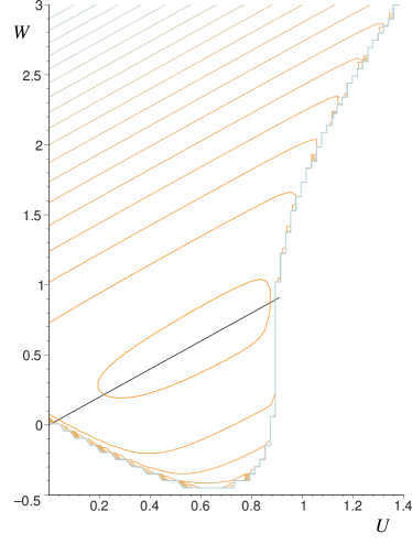
As Fig. 2 shows, the potential is positive definite and finite as long as we are inside the vector multiplet scalar manifold illustrated in Fig. 1. The potential diverges at the boundary $b_{2}$ where the vector multiplet metric $g_{xy}$ has a zero eigenvalue. At the boundary $b_{1}$, where $\det(g_{xy})$ is infinite, the potential is finite. This behavior can be traced back to the second term of the scalar potential (2.20) which contains the inverse metric $g^{xy}$.

There are, however, additional features of the potential, which cannot be inferred from Fig. 2 directly. While Fig. 2 clearly shows that the value of the potential is small in the vicinity of the flop line $U=W$, an explicit calculation reveals that its actual minimum (for these fixed values of the hypermultiplet scalars) is not located at the flop line but slightly next to it. One should also note that even though Fig. 2 suggests that this point is a critical point, this is not the case, since the derivatives of $\mathbbm{V}$ with respect to the hypermultiplet scalars do not vanish. Finally we observe that the potential diverges quadratically, $\mathbbm{V}\propto W^{2}$, in the limit $W\rightarrow\infty$.

After analyzing the behavior of the potential at the boundaries of the vector multiplet scalar manifold, we now turn to the boundaries appearing in the hypermultiplet sector. These are given by the loci where the hypermultiplet metric (3.45) has an infinite eigenvalue, due to $\phi_{+}$ or $\phi_{-}$ defined in (3.41) becoming zero. Assuming $v^{1}=u_{1}=0$ and $v^{2}=\bar{v}^{2}=p,u_{2}=\bar{u}_{2}=q$ to be real we obtain

$$\phi_{+}=1-p^{2}\,,\quad\phi_{-}=1-q^{2}+p^{2}\,q^{2}\,.$$ (4.21)

This shows that $p$ is bounded and takes values $-1<p<1$ while $q$ is unbounded. The dependence of the potential $\mathbbm{V}$ on the hypermultiplet scalars $p,q$ for frozen vector multiplet scalar fields is shown in Fig. 3.
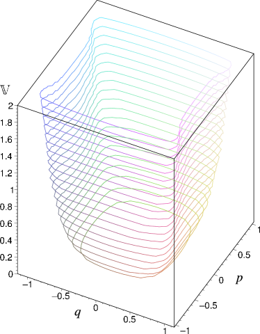
Refer to caption
Figure 3: The scalar potential restricted to the submanifold $U=W=0.6$, $v^{1}=u_{1}=0$, $v^{2}=\bar{v}^{2}=p$ and $u_{2}=\bar{u}_{2}=q$. The potential diverges at the boundaries where $\phi_{+}$ or $\phi_{-}$ become zero.

This figure illustrates that $\mathbbm{V}$ diverges at the boundaries of the hypermultiplet moduli space where $\phi_{+}$ or $\phi_{-}$ vanish. The minimum of the potential, $\mathbbm{V}_{\rm min}=0$, is located at $q=p=0$, which corresponds to the case of vanishing transition states.

Combined with the result obtained for the vector multiplet scalar manifold, this shows that the potential diverges at all boundaries of the moduli space where the scalar metrics develop a zero eigenvalue. At the boundary $U=0$, where $\det(g_{xy})$ is infinite the potential is finite.

5 General flop transitions

In the previous section we constructed the In-picture Lagrangian for a particular example of a flop transition where the transition states were given by a single charged hypermultiplet. We will now generalize this construction to a generic flop where $N$ hypermultiplets become massless at the transition locus. Our construction does not depend on the details of the vector multiplet scalar manifolds connected by the flop and can easily be adjusted to any specific transition. The relation between Out-picture and In-picture is given by the orbit sum rule (2.33). After fixing the hypermultiplet scalar manifold to be $X(N+1)$, we find that the resulting hypermultiplet sector of these In-picture Lagrangians is still uniquely determined by the microscopic theory.

5.1 Constructing the action

We will now construct the In-picture Lagrangians for a generic flop transition where the homology class $C^{\star}=q_{I}C^{I}$ contains $N$ isolated holomorphic curves. In this case the transition states are given by $N$ hypermultiplets, which are charged with respect to the vector field $A^{\star}_{\mu}=q_{I}A^{I}_{\mu}$ associated to $C^{\star}$.161616We do not assume that an adapted parametrization of the Kähler cone (where $h^{I}>0$) has been chosen. Generalizing our construction from the previous section, we take the hypermultiplet scalar manifold to be $X(N+1)$, which will contain the universal hypermultiplet $v^{1},u_{1}$ and $N$ charged hypermultiplets $v^{\alpha},u_{\alpha}$. Here the index $\alpha=2,\ldots,N+1$ enumerates the charged hypermultiplets which correspond to the transition states. We further use $h^{\star}=q_{I}h^{I}$ to denote the volume of the shrinking cycle $C^{\star}$.

The microscopic theory imposes that the transition states are charged with respect to $A^{\star}_{\mu}$, while the universal hypermultiplet remains neutral. This condition requires the existence of a holomorphic Killing vector of the form:

$$k^{v^{i}}_{\rm gauge}=-i\left[\,0\,,\,v^{2}\,,\,\ldots\,,v^{N+1}\,\right]^{\rm T}\,,\quad k^{u_{i}}_{\rm gauge}=i\left[\,0\,,\,u_{2}\,,\,\ldots\,,u_{N+1}\,\right]^{\rm T}\,.$$ (5.1)

Since this Killing vector is holomorphic, its components $k^{\bar{v}^{i}}_{\rm gauge}$ and $k^{\bar{u}_{i}}_{\rm gauge}$ can be obtained from $k^{v^{i}}_{\rm gauge}$ and $k^{u_{i}}_{\rm gauge}$ by complex conjugation. The sign conventions and overall scale in (5.1) are chosen such that for $N=1$ we reproduce the results of the previous section.

The first step is to check whether there exists a generator $t$ which gives rise to this Killing vector. By inspection of (3.2) we find this generator should correspond to an element of the Cartan subgroup of $SU(N+1,2)$, the isometry group of $X(N+1)$. This implies that $t$ should be diagonal. In this case the general expression for a Killing vector on $X(N+1)$ (3.2) simplifies to

$$\begin{split}k^{\zeta}&=0\,,\\ k_{z}&=\frac{i}{2}\left(t^{n+1}_{~{}~{}~{}n+1}-t^{n}_{~{}~{}n}\right)\,,\\ \hat{k}^{v^{i}}&=i\left(t^{i}_{~{}j}v^{j}-v^{i}\,t^{n+1}_{~{}~{}~{}n+1}\right)\,,\\ \hat{k}^{u_{i}}&=i\left(t^{n+1}_{~{}~{}~{}n+1}u_{i}-t^{j}_{~{}i}u_{j}-u_{i}\left(t^{n+1}_{~{}~{}~{}n+1}-t^{n}_{~{}~{}n}\right)\right)\,.\end{split}$$ (5.2)

Here it is implicitly understood that $t^{i}_{~{}j}=a_{k}\,\delta^{i}_{~{}j}$ is diagonal. The $a_{k}$ are $N+1$ real constants. Comparing coefficients between the eqs. (5.1) and (5.2), we find the following relations for the entries of $t$:

$$\begin{split}a_{1}=t^{n+1}_{~{}~{}~{}n+1}\quad,\quad-a_{\alpha}+t^{n+1}_{~{}~{}~{}n+1}=1\,&,\quad t^{n+1}_{~{}~{}~{}n+1}=t^{n}_{~{}n}\,,\\ a_{1}+\sum_{\alpha=2}^{N+1}a_{\alpha}+t^{n}_{~{}n}+t^{n+1}_{~{}~{}~{}n+1}=0\,.&\end{split}$$ (5.3)

The last equation arises from the condition that $t$ should be traceless. This set of equations has the unique solution:

$$t^{1}_{~{}1}=t^{n}_{~{}n}=t^{n+1}_{~{}~{}~{}n+1}=\frac{N}{N+3}\,,\quad t^{2}_{~{}2}=\ldots=t^{N+1}_{~{}~{}~{}~{}N+1}=-\,\frac{3}{N+3}\,.$$ (5.4)

Hence the gauge generator $t_{\rm gauge}$ is uniquely determined,

$$t_{\rm gauge}={\rm diag}\left[\frac{N}{N+3}\,,\underbrace{-\,\frac{3}{N+3}\,,\,\ldots\,,\,-\frac{3}{N+3}}_{N{\rm times}}\,,\,\frac{N}{N+3}\,,\,\frac{N}{N+3}\,\right]\,.$$ (5.5)

Observe that in the case $N=1$, this is exactly the generator (4.2) of our example.

In the next step we calculate the moment map for this isometry by substituting $t_{\rm gauge}$ into eq. (3.2). Taking linear combinations $\hat{\mu}^{1}=\hat{\mu}^{+}+\hat{\mu}^{-}$, $\hat{\mu}^{-}=-i\left(\hat{\mu}^{+}-\hat{\mu}^{-}\right)$ and using the definition (3.41) to simplify the resulting expressions, we obtain the following $SU(2)$ triplet of moment maps:

$$\hat{\mu}^{r}_{\rm gauge}=\left[\begin{array}[]{c}\frac{i}{2\phi_{+}^{1/2}\phi_{-}^{1/2}}\left(v^{\alpha}\,u_{\alpha}-\bar{v}^{\alpha}\bar{u}_{\alpha}\right)\\ \frac{1}{2\phi_{+}^{1/2}\phi_{-}^{1/2}}\left(v^{\alpha}\,u_{\alpha}+\bar{v}^{\alpha}\bar{u}_{\alpha}\right)\\ \frac{1}{2\phi_{-}}\left(\bar{u}_{\alpha}u_{\alpha}\right)-\frac{1}{2\phi_{+}}\left(\bar{v}^{\alpha}v^{\alpha}\right)\end{array}\right]\,.$$ (5.6)

The gauging of this isometry exactly proceeds as in the example of the previous section.

In order to complete the construction of our In-picture Lagrangians we still have to calculate the scalar potential. For this purpose we first derive the superpotential $\mathcal{W}$ (2.23). The moment map $P^{r}$ is given by

$$P^{r}=\frac{1}{2}\,h^{\star}\,\hat{\mu}^{r}_{\rm gauge}(q)\,.$$ (5.7)

Substituting in the explicit form of $\hat{\mu}^{r}_{\rm gauge}$, the superpotential $\mathcal{W}$ becomes

$$\mathcal{W}=\frac{1}{\sqrt{6}}\,h^{\star}\,\left(\left(\frac{1}{2\phi_{-}}\left(\bar{u}_{\alpha}u_{\alpha}\right)-\frac{1}{2\phi_{+}}(\bar{v}^{\alpha}v^{\alpha})\right)^{2}+\frac{1}{\phi_{+}\phi_{-}}\left(\bar{v}^{\alpha}\bar{u}_{\alpha}\right)\left(v^{\alpha}u_{\alpha}\right)\right)^{1/2}\,.$$ (5.8)

Looking at $Q^{r}$ defined in (2.24), we see that

$$Q^{r}=\sqrt{\frac{2}{3}}\,\frac{P^{r}}{\mathcal{W}}=\frac{\hat{\mu}^{r}_{\rm gauge}(q)}{\left(\hat{\mu}^{s}_{\rm gauge}(q)\hat{\mu}^{s}_{\rm gauge}(q)\right)^{1/2}}$$ (5.9)

is independent of the vector multiplet scalar fields and satisfies the condition $\partial_{x}Q^{r}=0$. Hence the scalar potential can be expressed in terms of the superpotential and takes the form (2.21).

5.2 Calculating the mass matrix

After constructing the effective Lagrangian which includes the transition states for a generic flop transition, we will now check that the masses of the scalar fields satisfy the conditions arising from the microscopic theory. We start by determining the vacuum of our theory. As in the $\mathbbm{F}_{1}$-model the equation

$$\partial_{\Lambda}\mathcal{W}=0$$ (5.10)

is solved by setting all transition states to zero. Corollary 3 of [45] assures that these are all critical points of the superpotential and therefore all supersymmetric critical points of $\mathbbm{V}$.171717The existence of further critical points of $\mathbbm{V}$ depends on the explicit choice of vector multiplet scalar manifold and is therefore not addressed here. The vacuum expectation values of the vector multiplet scalars and the universal hypermultiplet are not determined. With this observation we find the vacuum manifold $\mathcal{M}_{C}$ of our theory:

C={vα=uα=0,α=2,,N+1v1,u1,ϕx,not determined by eq. (5.10).subscript𝐶casessuperscript𝑣𝛼subscript𝑢𝛼0𝛼2𝑁1superscript𝑣1subscript𝑢1superscriptitalic-ϕ𝑥not determined by eq. (5.10).\mathcal{M}_{C}=\left\{\begin{array}[]{ll}\,v^{\alpha}\,=\,u_{\alpha}\,=0\,,&\alpha=2,\ldots,N+1\\ \,v^{1}\,,\,u_{1}\,,\,\phi^{x}\,,&\mbox{not determined by eq. (\ref{6.11}).}\end{array}\right. (5.11)

Substituting $\mathcal{M}_{C}$ into the superpotential, we find that $\mathcal{W}$ vanishes identically. Hence we have $\mathbbm{V}(\phi,q)|_{\mathcal{M}_{C}}=0$ and the vacuum is Minkowski. This is in complete analogy to our analysis in subsection 4.2.

We will now calculate the mass matrix (4.17) for our Lagrangian. In this case it is more convenient to start from the scalar potential in the form (2.20):

$$\mathbbm{V}(\phi,q)=-4P^{r}P^{r}+2g^{xy}P^{r}_{x}P^{r}_{y}+\frac{3}{4}g_{XY}K^{X}K^{Y}\,.$$ (5.12)

Here the first observation is that for the $P^{r}$ given in (5.7) the terms $P^{r}P^{r}$ and $g^{xy}P^{r}_{x}P^{r}_{y}$ are of fourth order in the transition states. This implies that these terms do not contribute to the mass matrix of our model since they vanish identically when taking two derivatives with respect to any scalar field and restricting to $\mathcal{M}_{C}$ afterwards. Hence the masses of our fields are solely generated by the last term in eq. (5.12).

In the next step we show that the vector multiplet scalar fields $\phi^{x}$ are massless. The matrix

$$\mathcal{M}_{\Lambda\Sigma}:=\left.\partial_{\Lambda}\partial_{\Sigma}\left(\frac{3}{4}\,{\rm g}^{2}\,g_{XY}\,K^{X}\,K^{Y}\right)\right|_{\mathcal{M}_{C}}$$ (5.13)

has non-trivial entries iff both $\Lambda$ and $\Sigma$ take values in the hypermultiplet sector. To see this, we expand $K^{X}=h^{\star}(\phi)k^{X}_{\rm gauge}(q)$ and note that $k^{X}_{\rm gauge}(q)$ vanishes when restricted to $\mathcal{M}_{C}$. This implies $\mathcal{M}_{\Lambda\Sigma}$ is only non-trivial if there is one derivative acting on each of the Killing vectors $k^{X}_{\rm gauge}(q)$. Since $g^{\Xi\Lambda}=g^{XY}\oplus g^{xy}$ is the direct sum of the hypermultiplet and vector multiplet inverse metrics, we find that non-trivial entries of the mass matrix (4.17) may occur in hypermultiplet sector only. This establishes that the vector multiplet scalars $\phi^{x}$ are massless.

Thus we restrict our analysis to the case where both $\Lambda$ and $\Sigma$ take values in the hypermultiplet sector and calculate the masses of the hypermultiplets. Only terms where each Killing vector is acted on by a derivative contribute to $\mathcal{M}_{XY}$:

$$\mathcal{M}_{WZ}=\left.\frac{3}{2}\,{\rm g}^{2}\,(h^{\star})^{2}\,g_{XY}\,\partial_{W}\,k^{X}_{\rm gauge}\,\partial_{Z}\,k^{Y}_{\rm gauge}\,\right|_{\mathcal{M}_{C}}\,.$$ (5.14)

The actual calculation of $\mathcal{M}_{XY}$ proceeds in two steps. We first calculate the matrix $K^{Y}_{~{}X}:=\partial_{X}k^{Y}_{\rm gauge}(q)|_{\mathcal{M}_{C}}$. With respect to the basis

$$q^{X}=\left\{\,v^{1}\,,\ldots,v^{N+1}\,,\,\bar{v}^{1}\,,\ldots,\,\bar{v}^{N+1}\,,\,u_{1}\,,\ldots,\,u_{N+1}\,,\,\bar{u}_{1}\,,\ldots,\,\bar{u}_{N+1}\,\right\}$$ (5.15)

$K^{Y}_{~{}X}$ is diagonal and has the following form:

$$K_{Y}^{~{}X}={\rm diag}\left[0,\underbrace{-i,\ldots,-i}_{N\,{\rm times}},0,\underbrace{i,\ldots,i}_{N\,{\rm times}},0,\underbrace{i,\ldots,i}_{N\,{\rm times}},0,\underbrace{-i,\ldots,-i}_{N\,{\rm times}}\right]\,.$$ (5.16)

In the second step we calculate $g_{XY}(q)|_{\mathcal{M}_{C}}$ by restricting the general expression for $g_{XY}(q)$ given in eq. (3.1) to $\mathcal{M}_{C}$. We find that all blocks appearing in (3.45) become diagonal. Taking into account the relation (3.77), their non-vanishing entries are given by

$$\begin{array}[]{ll}g_{v_{1}\bar{v}_{1}}=\frac{1}{2\phi_{+}^{2}\phi_{-}^{2}}\left(1-\bar{u}_{1}u_{1}\left(1-\bar{v}^{1}v^{1}\right)^{2}\right)\,,&g_{v^{\alpha}\bar{v}^{\beta}}=\frac{1}{2\phi_{+}}\,\delta_{\alpha\beta}\,,\\ g_{u_{1}\bar{u}_{1}}=\frac{1}{2\phi_{-}^{2}}\left(1-\bar{v}^{1}v^{1}\right)\,,&g_{u_{\alpha}\bar{u}_{\beta}}=\frac{1}{2\phi_{-}}\,\delta^{\alpha\beta}\,,\\ g_{\bar{v}^{1}u_{1}}=-\,\frac{1}{2\phi_{-}^{2}}\left(\bar{u}_{1}v^{1}\right)\,.&\end{array}$$ (5.17)

Here and in the following $\phi_{+}$ and $\phi_{-}$ are understood to be restricted to $\mathcal{M}_{C}$. The matrix $\mathcal{M}_{XY}$ can now be computed from

$$\mathcal{M}_{XY}=\,\frac{3}{2}{\rm g}^{2}\,(h^{\star})^{2}\left[K\,g\,K^{\rm T}\right]\,.$$ (5.18)

Explicitly, we find

$$\mathcal{M}_{XY}=\,\left[\begin{array}[]{cccc}0&A&0&0\\ A&0&0&0\\ 0&0&0&B\\ 0&0&B&0\\ \end{array}\right]\,,$$ (5.19)

with $A$ and $B$ being the following $(N+1)\times(N+1)$-dimensional block matrices:

$$A=\frac{3}{4\phi_{+}}{\rm g}^{2}(h^{\star})^{2}\;{\rm diag}\left[0,\underbrace{1,\ldots,1}_{N\,{\rm times}}\right]\,,\quad B=\frac{3}{4\phi_{-}}{\rm g}^{2}(h^{\star})^{2}\;{\rm diag}\left[0,\underbrace{1,\ldots,1}_{N\,{\rm times}}\right]\,.$$ (5.20)

Finally we need to calculate the inverse metric $g^{XY}$, restricted to $\mathcal{M}_{C}$, by inverting $g_{XY}|_{\mathcal{M}_{C}}$ given in (5.17). The resulting inverse metric is again of the structure (3.45) with block diagonal entries. The only non-zero components are given by

$$\begin{array}[]{ll}g^{v^{1}\bar{v}^{1}}=2\,\phi_{+}^{2}\,\phi_{-}\,,&g^{v^{\alpha}\bar{v}^{\beta}}=2\phi_{+}\delta^{\alpha\beta}\,,\\ g^{u_{1}\bar{u}_{1}}=2\,\frac{\phi_{-}}{\phi_{+}}\left(1-\bar{u}_{1}u_{1}\left(1-\bar{v}^{1}v^{1}\right)^{2}\right)\,,&g^{u_{\alpha}\bar{u}_{\beta}}=2\,\phi_{-}\,\delta^{\alpha\beta}\,,\\ g^{v^{1}\bar{u}_{1}}=2\phi_{+}\,\phi_{-}\left(\bar{u}_{1}v^{1}\right)\,.&\end{array}$$ (5.21)

The hypermultiplet masses are given by the eigenvalues of the mass matrix

$$\mathcal{M}^{X}_{~{}~{}Y}=\left.g^{XZ}\,\mathcal{M}_{ZY}\right|_{\mathcal{M}_{C}}\,.$$ (5.22)

Using the results (5.19) and (5.21), we find that the resulting matrix is diagonal

$$\mathcal{M}^{X}_{~{}Y}=(m_{t})^{2}\,\left[0,\underbrace{1,\ldots,1}_{N\,{\rm times}},0,\underbrace{1,\ldots,1}_{N\,{\rm times}},0,\underbrace{1,\ldots,1}_{N\,{\rm times}},0,\underbrace{1,\ldots,1}_{N\,{\rm times}}\right]^{X}_{~{}Y}\,,$$ (5.23)

where $(m_{t})^{2}=\frac{3}{2}\,(h^{\star})^{2}\,{\rm g}^{2}$. This result explicitly shows that our Lagrangian contains one massless hypermultiplet, given by the complex fields $v^{1},u_{1}$. This multiplet corresponds to the universal hypermultiplet. The transition states $v^{\alpha},u_{\alpha}$ all acquire the same mass

$$m_{t}=\sqrt{\frac{3}{2}}\,{\rm g}\,h^{\star}\,.$$ (5.24)

It is proportional to the volume of the flopped cycle, $h^{\star}$, as required by the underlying microscopic theory. Comparing (5.24) to eq. (2.31) we find that the gauge coupling constant ${\rm g}$ is again set by (4.20).

This result concludes the construction of the In-picture Lagrangian for a generic flop transition. We find that after fixing the hypermultiplet scalar manifold to be $X(N+1)$, the hypermultiplet sector of the resulting action is uniquely determined in terms of the microscopic theory. We further note that in order to calculate the mass matrix, we did not need to specify the details of the vector multiplet sector. Hence the analysis in this section can be used to model any flop transition where $N$ charged hypermultiplets become massless. In the case where $N=1$ these results exactly match the ones found in the explicit example given in section 4.

6 Discussion and Outlook

In this paper we have constructed a family of five-dimensional gauged supergravity actions which can be used to describe flop transitions in M-theory compactifications on Calabi-Yau threefolds. The new feature of these actions is that they explicitly include the extra light modes occurring in the transition region. The masses of these modes are encoded in the scalar potential. While the vector multiplet sector could be treated exactly, we used a toy model based on the Wolf spaces $X(1+N)=\frac{U(1+N,2)}{U(1+N)\times U(2)}$ to describe the hypermultiplets. In this context we worked out the metrics, the Killing vectors, and the moment maps using the superconformal quotient construction [31, 32, 33]. This geometrical data suffices to determine any hypermultiplet sector based on $X(1+N)$ in $\mathcal{N}=2$ supergravity in dimensions $d\leq 6$. Furthermore, this approach considerably simplifies the investigation of gaugings, as the Killing vectors and moment maps are directly given in terms of the generators of the isometry group of the underlying Wolf space.

Our low energy effective actions have all the properties required to model a flop transition. Only the transition states acquire a mass away from the flop and the potential has a family of degenerate supersymmetric Minkowski ground states, which is parametrized by the moduli of $X$. Therefore none of the flat directions is lifted, and there are no additional flat directions corresponding to Higgs branches. Note that this is not implied by the charge assignment alone. The scalar potential which encodes the masses of the scalar fields is a complicated function determined by the gauging. Here it was not obvious a priori that there exists a gauging which does not lift some of the flat directions or create new ones. The latter effect could arise through hypermultiplets combining with vector multiplets into long vector multiplets, giving rise to a Higgs branch. Thus it is non-trivial that we can model a flop transition with our quaternion-Kähler manifolds.

However, it is clear that a LEEA based on $X(1+N)$ can only be a toy model, as the hypermultiplet manifolds which actually occur in string and M-theory compactifications are unlikely to be symmetric spaces. Moreover, it is conceivable that integrating out the charged hypermultiplets modifies the couplings of the neutral hypermultiplets, so that the manifolds of the In-picture and the Out-picture are not related by the simple truncation $X(1+N)\rightarrow X(1)$. Yet, the very fact that we find a consistent description of a flop transition shows that while such threshold corrections might modify the couplings, they cannot play an essential role. This is different in the vector multiplet sector, where the threshold corrections play an essential role in determining the In-picture LEEA, because the Out-picture LEEA are discontinuous.181818 In the related case of $SU(2)$ enhancement it was proven in [17] that the Out-picture LEEA cannot be extended to an $SU(2)$ invariant action without taking into account the threshold corrections.

In summary, our model is a reasonable approximation of M-theory physics because it (i) defines a consistent gauged supergravity action, (ii) has, for arbitrary $N$, the correct properties to model a flop, (iii) is unique (once the hypermultiplet metric is fixed) and (iv) is simple enough to allow for explicit calculations. The last point will be illustrated in a separate paper [11], where we consider cosmological solutions.

One interesting direction of future research would be to take a complementary approach and ask for the constraints imposed on a general quaternion-Kähler manifold by the existence of a flop transition. This could also be helpful for deriving such metrics from M-theory calculations. Here we expect that again the description of quaternion-Kähler manifolds in terms of hyper-Kähler cones is useful.

Concerning the project [17, 18] of deriving LEEA for topological phase transitions and other situations with additional light states, the next step would be to consider conifold singularities in type II compactifications on Calabi-Yau threefolds. As this also involves additional massless hypermultiplets, we can use the same hypermultiplet sector as in this paper. The only complication is that the vector multiplet sector is much more involved, as it is encoded in a holomorphic instead of a cubic prepotential. Nevertheless, we expect that the threshold corrections can be treated along the lines of [18]. Further steps would be to consider phase transitions which have additional flat directions, such as conifold transitions and extremal transitions, and to include fluxes. The last point is of particular interest, since gaugings induced by flux are complementary to those related to transition states, as they involve non-compact isometries.

Ultimately, we need to know what are the most general gauged supergravity actions that can be obtained by the compactification of string or M-theory including all kinds of fluxes, branes and topological transitions. Only once this point has been mastered, we will have the technical tools to fully access the dynamics of transition states and to study their impact on problems such as moduli stabilization, inflation, and the naturalness problems associated with the electroweak scale and the cosmological constant.

Acknowledgments

We would like to thank B. de Wit, S. Vandoren and A. Van Proeyen for useful discussions. This work is supported by the DFG within the ‘Schwerpunktprogramm Stringtheorie’. F.S. acknowledges a scholarship from the ‘Studienstiftung des deutschen Volkes’. L.J. was also supported by the Estonian Science Foundation Grant No 5026.

References

  • [1] A. Strominger, Nucl. Phys. B451 (1995) 96, hep-th/9504090.
  • [2] E. Witten, Nucl. Phys. B471 (1996) 195, hep-th/9603150.
  • [3] P.S. Aspinwall, B.R. Greene, D.R. Morrison, Nucl. Phys. B416 (1994) 414, hep-th/9309097.
  • [4] E. Witten, Nucl. Phys. B403 (1993) 159, hep-th/9301042.
  • [5] B.R. Greene, D.R. Morrison, A. Strominger, Nucl. Phys. B451 (1995) 109, hep-th/9504145.
  • [6] B.R. Greene, in Fields, strings and duality, Boulder (1996) 543, hep-th/9702155.
  • [7] I. Gaida, S. Mahapatra, T. Mohaupt, W. Sabra, Class. Quant. Grav. 16 (1999) 419, hep-th/9807014.
  • [8] B.R. Greene, K. Schalm, G. Shiu, J. Math. Phys. 42 (2001) 3171, hep-th/0010207.
  • [9] T. Mohaupt, Fortschr. Phys. 51 (2003) 787, hep-th/0212200.
  • [10] M. Brändle, A. Lukas, Phys. Rev. D68 (2003) 024030, hep-th/0212263.
  • [11] L. Järv, T. Mohaupt, F. Saueressig, M-theory cosmologies from singular Calabi-Yau compactifications, hep-th/0310174.
  • [12] J. Polchinski, A. Strominger, Phys. Lett. B388 (1996) 736, hep-th/9510227. T.R. Taylor, C. Vafa, Phys. Lett. B474 (2000) 130, hep-th/9912152.
  • [13] G. Curio, A. Klemm, D. Lüst, S. Theisen, Nucl. Phys. B609 (2001) 3, hep-th/0012213.
  • [14] P. Mayr, Nucl. Phys. B593 (2001) 99, hep-th/0003198.
  • [15] S. Giddings, S. Kachru, J. Polchinski, Phys. Rev. D66 (2002) 106006, hep-th/0105097.
  • [16] J.L. Feng, J. March-Russel, S. Sethi, F. Wilczek, Nucl. Phys. B602 (2001) 307, hep-th/0005276.
  • [17] T. Mohaupt, M. Zagermann, JHEP 0112 (2001) 026, hep-th/0109055.
  • [18] J. Louis, T. Mohaupt, M. Zagermann, JHEP 0302 (2003) 053, hep-th/0301125.
  • [19] M. Wijnholt, S. Zhukov, Nucl. Phys. B639 (2002) 343, hep-th/0110109.
  • [20] J. Bagger, E. Witten, Nucl. Phys. B222 (1983) 1.
  • [21] M. Günaydin, G. Sierra, P.K. Townsend, Nucl. Phys. B242 (1984) 244, Nucl. Phys. B253 (1985) 573.
  • [22] M. Günaydin, M. Zagermann, Nucl. Phys. B572 (2000) 131, hep-th/9912027.
  • [23] A. Ceresole, G. Dall’Agata, Nucl. Phys. B585 (2000) 143, hep-th/0004111.
  • [24] J. Ellis, M. Günaydin, M. Zagermann, JHEP 0111 (2001) 024, hep-th/0108094.
  • [25] A.C. Cadavid, A. Ceresole, R. D’Auria, S. Ferrara, Phys. Lett. B357 (1995) 76, hep-th/9506144. G. Papadopoulos, P.K. Townsend, Phys. Lett. B357 (1995) 300, hep-th/9511108.
  • [26] I. Antoniadis, R. Minasian, S. Theisen, P. Vanhove, String loop corrections to the universal hypermultiplet, hep-th/0307268.
  • [27] S. Cecotti, S. Ferrara, L. Girardello, Int. J. mod. Phys A4 (1989) 2475.
  • [28] S. Ferrarra, S. Sabharwal, Nucl. Phys. B332 (1990) 317.
  • [29] P. Aspinwall, in Strings, branes and gravity, Boulder (1999) 723, hep-th/0001001.
  • [30] A. Swann, Math. Ann. 289 (1991) 421.
  • [31] B. de Wit, M. Roček, S. Vandoren, JHEP 0102 (2001) 039, hep-th/0101161.
  • [32] B. de Wit, M. Roček, S. Vandoren, Phys. Lett. B511 (2001) 302, hep-th/0104215.
  • [33] L. Anguelova, M. Roček, S. Vandoren, JHEP 0205 (2002) 064, hep-th/0202149.
  • [34] A. Ceresole, G. Dall’Agata, R. Kallosh, A. Van Proeyen, Phys. Rev. D64 (2001) 104006, hep-th/0104056.
  • [35] K. Galicki, Commun. Math. Phys. 108 (1987) 117. R. D’Auria, S. Ferrara, P. Fré, Nucl. Phys. B359 (1991) 705. L. Andrianopoli, M. Bertolini, A. Ceresole, R. D’Auria, S. Ferrara, P. Fré, T. Magri, J. Geom. Phys. 23 (1997) 111, hep-th/9605032. L. Andrianopoli, M. Bertolini, A. Ceresole, R. D’Auria, S. Ferrara, P. Fré, Nucl. Phys. B475 (1996) 397, hep-th/9603004.
  • [36] R. D’Auria, S. Ferrara, JHEP 0105 (2001) 034, hep-th/0103153.
  • [37] P.K. Townsend, Phys. Lett. B148 (1984) 55.
  • [38] P.M.H. Wilson, Invent. Math. 107 (1992) 561.
  • [39] T. Hübsch, Calabi-Yau manifolds, World Scientific, 1992.
  • [40] T. Oda, Convex bodies and algebraic geometry, Springer (1987).
  • [41] J. Louis, J. Sonnenschein, S. Theisen, S. Yankielowicz, Nucl. Phys. B480 (1996) 185, hep-th/9606049.
  • [42] A. Chou, R. Kallosh, J. Rahmfeld, S. Rey, M. Shmakova, W.K. Wong, Nucl. Phys. B508 (1997) 147, hep-th/9704142.
  • [43] N. Hitchin, A. Karlhede, U. Lindström, M. Roček, Commun. Math. Phys. 108 (1987) 535.
  • [44] J. Marsden, A. Weinstein, Rep. Math. Phys. 5 (1974) 121 .
  • [45] D. Alekseevsky, V. Cortés, C. Devchand, A. Van Proeyen, Flows on quaternionic-Kähler and very special real manifolds, hep-th/0109094.