On Bouncing Brane-Worlds, S-branes and Branonium Cosmology

Abstract:

We present several higher-dimensional spacetimes for which observers living on 3-branes experience an induced metric which bounces. The classes of examples include boundary branes on generalised S-brane backgrounds and probe branes in D-brane/anti D-brane systems. The bounces we consider normally would be expected to require an energy density which violates the weak energy condition, and for our co-dimension one examples this is attributable to bulk curvature terms in the effective Friedmann equation. We examine the features of the acceleration which provides the bounce, including in some cases the existence of positive acceleration without event horizons, and we give a geometrical interpretation for it. We discuss the stability of the solutions from the point of view of both the brane and the bulk. Some of our examples appear to be stable from the bulk point of view, suggesting the possible existence of stable bouncing cosmologies within the brane-world framework.

1 Introduction

Bouncing cosmologies have been advocated as having played a role in our past, both within pre-Big Bang cosmologies [1] for which new string-motivated physics smoothes out the Big Bang singularity, and within cyclic scenarios where the universe survives the passage through a succession of earlier singularities [2]. Interest in these proposals has been further sharpened by the recent precise measurements of temperature fluctuations in the cosmic microwave background (CMB). In particular, these models provide the main alternatives to the inflationary description of these fluctuations, motivating the detailed study of the kinds of late-time cosmologies to which they give rise.

A major obstacle to understanding their predictions arises from their potential dependence on the details of the bounce, and a study of this dependence has been hindered by the absence of a well-behaved model of a bouncing universe with which to test theoretical proposals. The difficulty with making such a model hinges on the necessity of violating the weak energy condition in order to do so, since this appears to inevitably require a physical instability to arise during the bouncing epoch.

Brane-world models permit a new approach to these difficulties, since they appear to allow the possibility that brane-bound observers might experience a bouncing universe, while embedded within a stable higher-dimensional geometry [3, 4, 5, 6, 7, 8, 9, 10, 11, 12, 13]. Ref. [6] pointed out such apparent example, consisting of a four dimensional cosmology based on a brane world embedded in a 5-dimensional Reissner-Nordström background. In this case, a solution for the appropriate junction conditions can be provided explicitly, with the result that the apparent weak energy condition violation term arises from the projection of bulk curvature effects onto the brane. This construction has recently been criticized, however, as inheriting the instability to fluctuations of the underlying Reissner-Nordström geometry [13].

Our purpose in this paper is to broaden the context of the discussion, by presenting a number of new brane-world constructions for which the brane-bound observers experience bounces. In particular we do so for geometries which do not require bulk electric fields, and which may not have the same stability problems which afflict the Reissner-Nordström example. We provide two classes of examples, which differ according to whether or not the relevant brane is a probe brane moving in a bulk spacetime, or is a boundary brane subject to an appropriate set of Israel junction conditions.

We present our results in the following way. In the next section we review the usual conditions which are required in order for four-dimensional FRW cosmologies to bounce. In particular, we focus on the case of universes with negative or flat curvature, in which the bounce requires a violation of the weak energy condition, leading to non-standard acceleration. Section 3 then describes several models with bounce having boundary 3-branes moving in various five-dimensional geometries. These examples include simple $S$-brane-like geometries which are solutions to the Einstein equations, as well as examples which also involve bulk dilatons and gauge fields. The resulting background geometries typically have either time-like or space-like singularities as well as Cauchy horizons. For each model, we identify the terms that appear in the effective four dimensional Friedmann equation, which are responsible for the bouncing behavior. Section 4 presents similar models based on observers riding probe branes within bulk spaces whose dimension can be higher than 5. These move through field configurations which solve higher-dimensional supergravity equations, and which represent the field sourced by a stack of source branes. Being supersymmetric, these bulk configurations are stable. Finally, our conclusions are summarized in section 5.

2 Bouncing and Acceleration in Standard Cosmology

We start by reviewing the conditions for a bouncing behavior which arise within 4D standard cosmology (see also, for example, [14]). We express these requirements in terms of the various energy conditions which the energy density in the universe must satisfy (or violate) in order to obtain a bounce. As we shall see, the same energy conditions also turn out to be quite useful for understanding bouncing behaviors in non-standard cosmologies based on extra-dimensional models.

For our purposes, the universe bounces when it passes smoothly from a contracting to an expanding phase without encountering an intervening singularity. That is, the universal scale factor, $a(t)$, reaches a positive, minimum value $a_{0}>0$ in the past, at a time which we choose to be $t=0$. This turning point separates contraction from expansion, and a necessary condition for its existence is that the universe experiences positive acceleration, $\ddot{a}>0$, for some interval around the turning point. The conditions for bouncing are consequently intimately related to those for positive acceleration.

2.1 Basic equations and energy conditions

In standard cosmology, a metric which preserves the observed homogeneity and isotropy in the three spatial dimensions has an FRW form, and we restrict ourselves to this form from now on:

$$ds^{2}=-d\tau^{2}+a^{2}(\tau)\,d\Omega^{2}_{k,3}\,.$$ (1)

Here $d\Omega^{2}_{k,3}=dr^{2}/(1-kr^{2})+r^{2}\,d\Omega_{2}^{2}$ is the usual metric on the spatial slices, with $d\Omega^{2}_{2}$ denoting the line element on the 2-sphere. The constant $k$ takes one of the three values $k=0$ or $\pm 1$ for flat, spherical or hyperbolic spatial topologies.

Homogeneity and isotropy imply the stress-energy density of matter must have the perfect-fluid form:

$$T_{\mu}^{\,\,\nu}=\hbox{diag}\,\left(-\rho,\,p,\,p,\,p\right)\,,$$ (2)

with, as usual, $p$ and $\rho$ being the fluid’s pressure and energy density. We assume these to be related by an equation of state of the form

$$p\,=\,\omega\rho\,$$ (3)

with the parameter $\omega$ being constant.

Assuming the metric evolution to be governed by Einstein’s equations, the cosmological evolution of the the universe is then given by the usual three equations,

• The equation of conservation of energy:

  $$\dot{\rho}+3\,H\,(\rho+p)\,=\,0\,\,,$$ (4)

• The Friedmann equation

  $$H^{2}+\frac{k}{a^{2}}=\frac{8\pi G_{4}}{3}\rho$$ (5)

• The Raychaudhuri equation

  $$\frac{\ddot{a}}{a}=-\frac{4\,\pi G_{4}}{3}(\rho+3p)\,.$$ (6)

Here $G_{4}$ denotes the four-dimensional Newton’s constant and the Hubble parameter is, as usual, $H\equiv{\dot{a}}/{a}$. These equations clearly tie the cosmic acceleration of the universe to the energy and pressure of the matter it contains. We now summarize several energy conditions which have been proposed to characterize reasonable general conditions for how the pressure and energy of stable matter can behave [15, 16].

• The weak energy condition (WEC), states that $T_{\mu\nu}t^{\mu}t^{\nu}\geq 0$ for any time-like vector $t^{\mu}$. This condition states that energy density measured by any observer is non-negative. Equivalently, in terms of energy density and pressure, $\rho\geq 0$ and $\rho+p\geq 0$. The validity of WEC is in general crucial for the proof of singularity theorems.

• The dominant energy condition (DEC), requires the same constraints as does the WEC, with in addition the requirement that $T^{\mu\nu}t_{\mu}$ cannot be space-like. This translates into the condition $\rho\geq|p|$ or $1\geq\omega$. When the DEC is satisfied, the conservation theorem by Hawking and Ellis applies [15], which shows that energy cannot propagate outside the light cone (and so, in particular, energy-momentum cannot spontaneously appear from nothing).

• The strong energy condition (SEC), requires that $T_{\mu\nu}t^{\mu}t^{\nu}\geq\frac{1}{2}T_{\lambda}^{\lambda}\,t^{\sigma}t_{\sigma}$ for all time-like vectors $t^{\mu}$. Equivalently, $\rho+p\geq 0$ and $\rho+3p\geq 0$.

2.2 Conditions for Bouncing

A bounce requires $\dot{a}$ to pass smoothly from negative to positive values, and so it follows that $H$ must vanish at some (turning) point, around which $\ddot{a}>0$ and $a>0$. Eq. (6) shows that $\ddot{a}/a>0$ implies $p<-\rho/3$, and so a bounce necessarily implies a violation of the SEC.

Similarly, given the Friedmann equation, eq. (5), the vanishing of $H$ implies conditions on the energy density during the bounce. The precise condition depends on the curvature, $k$, of the three-dimensional spatial slices, as we now summarize.

Bouncing conditions when $k=1$:

This option is a textbook case, and in this instance a bounce requires the energy density to violate the strong energy condition (but not necessarily the WEC since $\rho$ need not pass through zero even if $H$ does). So in this case the condition $p<-\rho/3$ suffices, and no additional conditions need be imposed on $\rho$. (For the equation of state, (3), the condition $p<-\rho/3$ implies $\omega<-\,\frac{1}{3}$.) The classic example of this type is furnished by the de Sitter universe, for which $-p=\rho>0$.

Bouncing conditions when $k=0,-1$:

This case is more difficult to achieve and so is less well studied. It is not enough to have $p<-\rho/3$ to have a bounce, because the energy must also pass through zero (if $k=0$) or become negative (if $k=-1$). In addition to violating the SEC, a bounce also requires the energy density must violate the WEC (and consequently also the DEC). It is noteworthy that once $\rho<0$ the condition $p<-\rho/3$ becomes weaker, since it allows positive $p$. (For instance, for the equation of state, (3), $\rho<0$ and $p<-\rho/3$ implies $\omega>-\,\frac{1}{3}$ rather than $\omega<-\,\frac{1}{3}$.)

Since the kinematics of this kind of bounce is less familiar, we next examine this case in more detail, assuming an equation of state, (3), with constant $\omega$. Energy conservation, (4), for these theories gives rise to the relation

$$\rho=\rho_{0}\,\left(\frac{a(\tau)}{a_{0}}\right)^{-3(1+\omega)}=-c\cdot\,a^{-3(1+\omega)}(\tau)\,,$$ (7)

where $c=-\rho_{0}/a_{0}^{-3(1+\omega)}$. Since we imagine $\rho_{0}<0$ at the turning point, we take $c>0$.

If we assume for concreteness that $k=-1$, the Friedmann equation can be written as

$$\dot{a}^{2}=1-c\,a^{-(1+3\omega)}\,.$$ (8)

where $c$ is the parameter defined in (7). From this equality it is clear that the scale factor never becomes smaller than $a_{min}=c^{1/(1+3\omega)}$, and $\dot{a}=0$ when $a=a_{min}$. It is not difficult to see that the universe bounces at this minimum value. For example, in the special case $\omega=\frac{1}{3}$, one can solve eq. (8) analytically to find

$$a^{2}(\tau)=\tau^{2}+c\,.$$ (9)

The resulting space-time is not singular for any finite $\tau$.

The Raychaudhuri equation, for the system we are considering, takes the form

$$\frac{\ddot{a}}{a}=\frac{4\,\pi\,c\,G_{4}}{3}(1+3\omega)\cdot\,a^{-3(1+\omega)}(\tau)\,,$$ (10)

from which it is clear that $\omega>-\,\frac{1}{3}$ ensures the acceleration is always positive (although it asymptotically vanishes).

Not surprisingly, the causal structure of a bouncing universe such as this $k=-1$ example differs from the usual situation for expanding FRW cosmologies. In particular, an observer in the bouncing cosmology does not have a horizon which limits the distances from which she can receive signals. By definition, an observer has a horizon when the following integral converges:

$$\Delta\equiv\int_{t_{0}}^{+\infty}\frac{dt}{a(t)}<\infty\,,$$ (11)

since $\Delta$ represents the maximal distance that an observer at time $t_{0}$ can probe. In the above $k=-1$ example, using (5), we can write

$$\Delta=\int_{t_{0}}^{+\infty}\frac{dt}{a(t)}\\ =\int_{a_{0}}^{+\infty}da\,\frac{a^{{(-1+3\omega)}/{2}}}{\sqrt{a^{1+3\omega}+c}}\,.$$ (12)

It is simple to check that this expression diverges, regardless of the sign of $c$, provide $\omega>-\frac{1}{3}$. Consequently we obtain a system having eternal positive acceleration (although it vanishes asymptotically) without horizons.

This behavior is in marked contrast with the eternal positive acceleration that one meets in a de Sitter universe. The presence of horizons in the de Sitter case has been argued to mean that the total number of degrees of freedom contained in a causal patch of the universe is always finite, an observation which is regarded as having problematic consequences for field theory and string theory [17, 18]. We see that, for $k=-1$, we have acceleration without this horizon problem, and we provide in the next section, brane world examples with this characteristic.

2.3 Bouncing Brane Cosmologies

The new ingredient which branes introduce into the bouncing discussion is the potential they bring for separating the requirement for negative energies from the necessity for having an instability. They do so basically because there is more than one metric which appears in the physics of observers on a brane, and the metric which shows the bounce need not be the metric which appears in the Einstein action. We briefly summarize these issues here, before discussing several examples of bouncing branes in subsequent sections.

The distinction between the various metrics which are relevant to brane observers is most starkly highlighted in the situation where a brane moves through a static bulk spacetime — the so-called ‘mirage cosmology’ [19, 20]. In this case the induced metric, $\gamma_{\mu\nu}$, on the brane is typically time-dependent, because of its dependence on the time-dependent brane position, $y^{M}(t)$:

$$\gamma_{\mu\nu}=g_{MN}\,\partial_{\mu}y^{M}\,\partial_{\nu}y^{N}\,.$$ (13)

Since it is the induced metric which governs the propagation of particles living on the brane (like photons), for all observations performed by brane observers using these particles this time dependence would be indistinguishable from what would be seen from a stationary brane sitting in a time-dependent bulk spacetime.

On the other hand, the metric which appears in the low-energy effective 4D Einstein equation is the lowest Kaluza-Klein mode of the bulk metric, $g_{\mu\nu}$, and this in general differs from $\gamma_{\mu\nu}$. A brane observer can detect the difference between these two metrics since this difference generates a host of preferred-frame effects, which can be constrained even within the gravitational sector [21].

In this situation a new interpretation of the Friedmann equation becomes possible, and this is what allows the presence of negative-energy terms in it to be potentially benign. To this end consider the interpretation of a brane observer who is unaware of the difference between the two metrics, and who (like us) simply sees particles like photons propagating within a time-dependent metric. For isotropic and homogeneous spacetimes, the resulting blue/redshifts of the photons would be interpreted as being due to an FRW cosmology whose Hubble parameter, $H$, could be computed. Not knowing the distinction between $\gamma_{\mu\nu}$ and $g_{\mu\nu}$, this observer would interpret any dependence of $H^{2}$ on the scale factor, $a$, as being due to the presence of various forms of energy density, through the Friedmann-like formula (79). In particular, if the induced metric for this observer bounces, the observer would believe there must be negative energy present, as discussed above. The brane observer could similarly deduce the pressure of the various cosmological fluids using either conservation of energy or the Raychaudhuri equation [19].

The bulk observer would recognize that there is no real negative-energy field associated with the apparent bounce as seen by the brane observer, and so there also need not be any instability associated with it. Recognizing that there are two metrics in the problem, the bulk observer would see that these permit the definition of two scale factors, $a_{g}$ and $a_{\gamma}$. Although the bulk Einstein-Hilbert action implies the Friedmann equation in the usual way for $a_{g}$, it is only an ‘effective’ Friedmann equation for $a_{\gamma}$ which the brane observer determines from photon observations. (We call the Friedmann equation for $a_{\gamma}$ ‘effective’ because the kinetic term for $\gamma_{\mu\nu}$ comes partially from the brane kinetic energy, rather than purely from the Einstein-Hilbert action.) What the brane observer would say is a strange type of dark energy which does not couple to the visible fields on the brane, the bulk observer understands to be an artifact of the brane observer’s making observations using particles which are confined to a moving brane universe; on the other hand, the bulk observer is able to interpret these brane terms as due to particular properties of the higher dimensional system, that is not possible to realize at the level of projected lower dimensional physics.

It is this loop-hole which we wish to explore with the examples we provide in this paper. We also believe that the analogy between the misguided brane observer and the present-day evidence for dark energy is sufficiently uncomfortable to warrant a more systematic study of preferred-frame and gravity-wave effects in post-BBN cosmology.

3 Bouncing Boundary Branes

We have seen that for $k=0,-1$ cosmologies — which are often the ones of current interest — bouncing requires a violation of WEC and of DEC (which is to say vanishing or negative energy density for some observers). In the recent literature, systems that violate the DEC have been considered (see for example [22]), but they often result, in instabilities [16].

The new feature of brane-world models is the possibility which they raise of allowing bounces without necessarily paying the price of instability. Although observers on the brane do see a cosmological ‘fluid’ which violates DEC, this fluid is the projection of bulk curvature onto the brane. And so long as the full bulk theory is stable, it may be that this 4D DEC violation need not necessarily imply an instability of the full theory. Our goal in the remainder of this paper is to provide examples of brane-world models using spacetimes which appear to be stable.

The original proposal along these lines argues that an observer confined on a brane embedded into a five dimensional Reissner-Nordström geometry experiences a $k=0,\pm 1$ bounce for some brane trajectories [6, 10]. This observer finds source terms in her effective 4D Friedmann equation which appears to have negative energy, in agreement with the arguments of the previous section. Seen from the 5-dimensional perspective, these terms arise as bulk curvature contributions which are projected onto the brane. For the Reissner-Nordström example they are nonzero when the 5D black hole carries nonzero charge, and are zero otherwise. For vanishing charge the WEC-violating terms disappear, and the model has an initial singularity (at least when $k=0$ or $-1$).

The purpose of presenting these examples is to broaden the discussion of the connections between bounces, singularities and instabilities. For instance, bulk stability has been partially studied for some of the $S$-brane-like examples we provide in this section, with some indications that they may not share the bulk instabilities of the Reissner-Nordström geometry. The examples we provide also show that boundary-brane bounces are possible for pure gravity (with a cosmological constant) and so the presence of an electric charge in the background is not required. Instead, a feature which all of the examples of this section share with the Reissner-Nordström example is the presence of naked (time or space-like) singularities in the bulk spacetime, and this makes it difficult to rule out instabilities which arise due to fluctuations which propagate out of these singularities and reach the brane. This is likely related to the violation of the dominant energy condition (DEC) which the 4D observer sees, since this energy condition is used in the proof that energy and momentum cannot appear acausally, from outside the observer’s light cone.

In the remainder of this section we first review the origin of these WEC-violating contributions to the effective Friedmann equation, and then use the results to examine several new co-dimension one brane-world scenarios.

3.1 Boundary Branes and the Effective Friedmann Equation

Consider a five-dimensional bulk space time, $M$, that contains ($3+1)$-dimensional branes, $B$, on which 4-dimensional observers may be forced to live. We further imagine that these branes are boundary branes, $B=\partial M$, which we realize by imagining taking two copies of $M$ on one side of $B$, and gluing these together at $B$ to define a covering space for which the two sides of the brane are identified by a ${\mathbb{Z}}_{2}$ symmetry.

The back-reaction of the brane onto the geometry of the spacetime is obtained by requiring the system to satisfy appropriate matching conditions which relate the stress energy on the brane to the discontinuity of the geometry across the brane. The relevant discontinuity is in the extrinsic curvature, ${\mathcal{K}}_{MN}=\nabla_{M}\eta_{N}$, where $\eta_{N}$ is the unit normal to the brane. The discontinuity condition states [23]

$$\Delta{\mathcal{K}}_{\mu\nu}\equiv{\mathcal{K}}_{\mu\nu}^{+}-{\mathcal{K}}_{\mu\nu}^{-}=-\kappa_{5}^{2}\,\left(\tilde{T}_{\mu\nu}-\frac{1}{3}\tilde{T}^{\lambda}_{{}\lambda}\gamma_{\mu\nu}\right)\,,$$ (14)

where $\tilde{T}_{\mu\nu}$ denotes the stress energy of matter on the brane, and $\gamma_{\mu\nu}$ is the induced metric on the brane.

Explicitly, consider the following ansatz for the five-dimensional metric

$$ds_{5}^{2}=-h(r)\,dt^{2}+\frac{dr^{2}}{g(r)}+r^{2}d\,\Omega_{k,3}^{2}\,,$$ (15)

where as before $d\,\Omega_{k,3}^{2}$ represents the measure of a maximally symmetric three-dimensional subspace of constant curvature $k$. Different kinds of horizons for this metric correspond to null surfaces, $r=r_{h_{i}}$, along which $g(r)$ vanishes (provided these are not also curvature singularities). When such horizons exist $h$ and $g$ typically change sign, and this can change the geometry’s Killing vectors from being spacelike to being timelike (or vice-versa). In particular the metric is static (with $t$ as the time coordinate) if $h$ and $g$ are both positive, but it is explicitly time-dependent (with $r$ as the time coordinate) if $h$ and $g$ are both negative.

A simple choice for a 3-brane position is along a surface $r=r_{b}(t)$. Given this choice the induced four-dimensional metric is then completely specified to be

$$ds^{2}_{induced} = -\left[h(r_{b})-\frac{1}{g(r_{b})}\left(\frac{dr_{b}}{dt}\right)^{2}\right]\,dt^{2}+r_{b}^{2}\Omega_{k,3}^{2}$$ (16)

$$= -d\tau^{2}+a(\tau)^{2}d\,\Omega_{k,3}^{2}\,,$$

from which we see the brane’s proper time is given by $d\tau/dt=\left[h-({r^{\prime}}_{b}^{2}/g)\right]^{1/2}$, the induced scale factor is $a(\tau)=r_{b}[t(\tau)]$ and so the resulting Hubble parameter is $H=\dot{a}/a=(r^{\prime}_{b}/r_{b})\left[h-({r^{\prime}}_{b}^{2}/g)\right]^{-1/2}$. Notice that the derivative ${r^{\prime}}_{b}={dr_{b}}/{dt}$ vanishes if the brane sits at a fixed coordinate position, $r=r_{b}$, in a static geometry and so $H$ vanishes in this limit. On the other hand, $r^{\prime}_{b}\to\infty$ if the brane sits at a fixed coordinate (spacelike) position, $t=t_{b}$, in a time-dependent geometry, and in this case $H\to|g|^{1/2}/r_{b}$.

Since ${r^{\prime}}_{b}$ determines the brane’s extrinsic curvature, the trajectory, $r_{b}(t)$, is fixed in terms of the stress energy on the brane by the junction conditions, (14). Thus, the cosmological evolution in four dimensions, obtained by solving the junction conditions at the singular surface, has a clear geometrical interpretation in the motion of the brane along a time-like trajectory in the higher dimensional background [20].

Let us use the junction condition (14) to determine the form of the effective Friedmann equation as seen by an observer riding on the brane in our background. The extrinsic curvature can be written as

$${\mathcal{K}}_{\mu\nu}=\frac{1}{2}\eta^{\sigma}\ \frac{\partial\gamma_{\mu\nu}}{\partial x^{\sigma}}$$ (17)

and, in our case, we take $\eta^{\sigma}=\pm\,(\,(hg)^{-1/2}\,\dot{r}_{b},\,(hg)^{1/2}\,\dot{t},\,0,\,0,\,0)$, and $\dot{r}$ and $\dot{t}$ are derivatives with respect the proper time $\tau$. There are two nontrivial junction equations arising from the time and space components of (17). The spatial components of the extrinsic curvature can be found to be

$${\mathcal{K}}_{ij}\,=\,r_{b}\,g^{1/2}\,\sqrt{1+\frac{\dot{r}_{b}^{2}}{g}}\,\gamma_{ij}\,,$$ (18)

When the energy density on the brane has a perfect fluid form, and there is no direct coupling between bulk fields and brane matter besides gravity, the conservation of energy momentum tensor on the brane lead to the the energy conservation equation (4) for the energy density on the brane . It turns out that the time component of the extrinsic curvature, gives a third, non independent equation, so we need only to consider the spatial components as well as the energy conservation equations as evolution equations.

Assuming, again, that there is no direct coupling between bulk fields (besides gravity) and brane matter, the spatial components of the Israel junction conditions, obtained from (18), gives us the effective Friedmann equation on the brane:

$$\frac{\dot{a}^{2}}{a^{2}}=\frac{\kappa_{5}^{4}\,\rho^{2}}{36}-\frac{g(a)}{a^{2}}\,,$$ (19)

As it is clear from this formula, it is the term proportional to $g(a)$ which can give rise to negative contributions to the energy as seen by a brane observer.

It is useful to write eq. (19) in a way which is more suitable for both a numerical or qualitative approach. Writing

$$\dot{a}^{2}+W(a)=0\,,$$ (20)

where

$$W(a)\,=\,g(a)-\rho^{2}\,a^{2}\,,$$ (21)

the Friedmann equation is reduced to a Hamiltonian constraint for a particle having zero energy [13]. The potential $W(a)$ must be non-positive in order to have a solution of (20). It turns out that the solution has a bounce if $W$ vanishes for some scale factor, $a_{t}$, greater than zero, corresponding to a classical turning point of the particle motion. To decide if a cosmological model bounces, it suffices to plot the function $W$. This also provide us with constraints on the model parameters which have to be satisfied in order to get a bounce.

In the next sections, we present various new examples of brane-world models with a bouncing behavior. Our aim is mainly to describe the bouncing phase of the history of these universes; for this reason, in general we do not discuss the subsequent cosmological evolution in these models.

3.2 Pure Gravity S0-Brane Examples

In this section we provide additional examples of bouncing, co-dimension 1 brane worlds which are similar in spirit to the Reissner-Nordström proposal of ref. [6, 10]. A motivation for examining more solutions comes from the recent observation that the Reissner-Nordström brane-world model shares the instability of the underlying 5D geometry to back-reaction from fluctuations near the black-hole horizon [13]. As such it cannot decide the stability issue.

Consider first five-dimensional gravity with a negative cosmological constant,

$$S_{5}=\int d^{5}x\,\sqrt{-g}\left[\frac{1}{2\kappa_{5}^{2}}R+12\,\Lambda\right]\,+S_{4}\,,$$ (22)

where $S_{4}$ is the action of a four brane embedded in the full five-dimensional space-time and $\Lambda$ is positive. The solution of interest to Einstein’s equations in the bulk is

$$ds_{5}^{2}=-h(r)\,dt^{2}+\frac{dr^{2}}{h(r)}+r^{2}d\,\Omega_{-1,3}^{2}$$ (23)

with

$$h(r)=-1+\frac{\xi^{2}}{r^{2}}+\Lambda r^{2}\,,$$ (24)

where $\xi$ is an integration constant which is physically interpreted as measuring the tension of the time-like singularities which source the gravitational field. Notice that the surfaces of constant $t$ and $r$ are negatively curved.

If $4\Lambda\xi^{2}<1$ this geometry has two horizons, at $r=r_{\pm}$ with $2\Lambda r_{\pm}^{2}=1\pm\sqrt{1-4\Lambda\xi^{2}}$. Writing $h(r)=\Lambda(r^{2}-r_{+}^{2})(r^{2}-r_{-}^{2})/r^{2}$ shows that $h>0$ (and so the metric is static) for $r>r_{+}>r_{-}$ and $r<r_{-}<r_{+}$, but $h<0$ (and so the metric is time-dependent) if $r_{-}<r<r_{+}$. The resulting causal structure can be represented by a Penrose diagram which looks like that of an AdS-Reissner-Nordström black hole. For $\Lambda=0$, this background corresponds to an S0-brane geometry largely discussed in [24, 25, 26].

The effective Friedmann equation for an observer bound to a brane moving along a trajectory $r=r_{b}(t)$ (or $t=t_{b}(r)$) in this geometry takes the form

$$H^{2}=\rho^{2}-\frac{h(a)}{a^{2}}\,,$$ (25)

where $a(\tau)=r_{b}(\tau)$ and $\kappa_{5}^{2}=6$. Writing the energy density on the brane as $\rho=\lambda+\rho_{m}$ with $\lambda$ constant, eq. (25) becomes

$$H^{2}=2\lambda\rho_{m}+\rho_{m}^{2}+(\lambda^{2}-\Lambda)+\left[\frac{1}{a^{2}}-\frac{\xi^{2}}{a^{4}}\right]\,.$$ (26)

We identify the terms appearing in the RHS of (26) as follows. The first term has to form of the standard, linear term in $\rho_{m}$, provided we define an effective Newton’s constant in terms of the brane tension. The second is the now-familiar quadratic correction in $\rho_{m}$, the third term, between normal parenthesis, comes from the cosmological constants in the bulk and on the brane. The fourth term is the usual contribution that comes because our spatial slices have negative curvature. The final term is induced from the bulk and is the one which is most important for our discussion, since it looks like a negative contribution to the energy which scales with $a$ like radiation (i.e. with $\omega=\frac{1}{3}$). This term is precisely of the form discussed in Section (2) which is required if the brane observer is to see a bounce.

We now concentrate on two interesting special cases. The first is the simplest brane-world model that gives a bounce, consisting of a tensionless brane embedded in an empty bulk. The second is a more realistic model that contains energy density on the brane in the form of radiation. In both these two examples, an observer on the brane probes physics in a frame in which the Planck mass is constant in time.

A Simple Special Case

As our first example, consider a tensionless, empty brane embedded in a pure S-brane background. Since we seek simple examples of bounces rather than realistic descriptions of the present-day universe, we take $\Lambda=\lambda=\rho_{m}=0$ in the previous example. The absence of stress-energy on the brane ensures the brane world-sheet must embed into spacetime with vanishing extrinsic curvature, and inspection of eq. (18) shows that this is only possible if $h(r_{b})<0$ and $\dot{r}^{2}=|h(r_{b})|$. This corresponds to the brane lying in the time-dependent regions of the bulk, sweeping out a surface of constant spatial coordinate, $t_{b}$. The Penrose diagram for such a brane-world is shown in Figure 1.

In this case, eq. (25) reduces to

$$H^{2}=+\frac{1}{a^{2}}-\frac{\xi^{2}}{a^{4}}\,,$$ (27)

which can be integrated analytically, leading to

$$a^{2}(\tau)=\tau^{2}+\xi^{2}\,.$$ (28)

The acceleration of the scale factor is everywhere positive, vanishing only asymptotically:

$$\frac{\ddot{a}}{a}=\frac{\xi^{2}}{(\tau^{2}+\xi^{2})^{2}}\,.$$ (29)

The resulting cosmology has positive acceleration at any finite time, without the horizon problem as discussed after formula (12).

From these expressions it is clear that the scale factor never vanishes, so the 3-brane has a smooth bounce that crosses the intersection point between the Cauchy horizons. This bouncing geometry may be traced to the time-like singularities which source the bulk metric, since it is the non-standard term proportional to $\xi^{2}$ which is responsible. If the singularities are eliminated by sending $\xi\to 0$, the model becomes a standard negative-curvature-dominated empty universe, with the usual singularity at the origin.

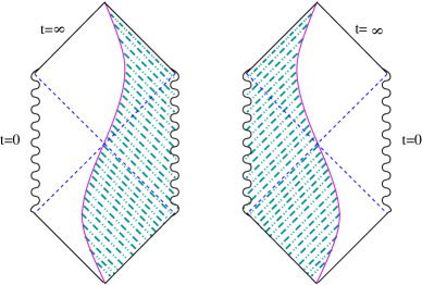
Figure 1: Graphical representation of a brane-world embedded in an S-brane background.

Stability against Perturbations

The stability of the bulk spacetime has been studied with mixed results. Although ref. [24, 26] found the geometry to be unstable to general perturbations, ref. [28] has pointed out that it is stable if fields are assigned initial conditions having compact support in the remote past. It is not yet known whether physical considerations can decide which set of boundary conditions should be used, or if instabilities may be generated by perturbations which propagate in along the horizon from the time-like singularities.

The same issues arise when the boundary brane is present, and these ensure the spacetime is stable against fluctuations which are confined to the brane (since these have compact support in the past, when viewed from the bulk). To see this explicitly let us evolve the fluctuations of a brane-bound massless, minimally-coupled scalar field, $\phi$, using the induced brane metric, whose amplitude is small enough that it does not significantly change the cosmological evolution of the background [6].

Using conformal time, the induced metric seen by the scalar field is

$$ds_{4}^{2} \equiv a^{2}(\eta)\left[-d\eta^{2}+d\Omega_{-1,3}^{2}\right]$$ (30)

$$= \xi^{2}\cosh^{2}{\eta}\left[-d\eta^{2}+d\Omega_{-1,3}^{2}\right]\,,$$

and the equation of motion for a fluctuation mode, $v_{k}=a\,\delta\phi_{k}$, with a given co-moving momentum, $k$, becomes

$$v_{k}^{\prime\prime}+\left(k^{2}-\frac{a^{\prime\prime}}{a}\right)v_{k}=0\,.$$ (31)

Here primes denote differentiation with respect to $\eta$, and for the metric under consideration $a(\eta)=\xi\,\cosh\eta$, so $a^{\prime\prime}/a=1$.

The WKB solutions for modes not near $k^{2}=1$, is

$$\delta\phi_{k}^{\pm}=\frac{v^{\pm}_{k}}{a} = \frac{e^{\pm i\eta\sqrt{k^{2}-1}}}{a(\eta)\left[2\sqrt{k^{2}-1}\right]^{1/2}}\qquad\hbox{if}\quad|k|>1\,,$$ (32)

$$= \frac{e^{\pm\eta\sqrt{1-k^{2}}}}{a(\eta)\left[2\sqrt{1-k^{2}}\right]^{1/2}}\,\qquad\hbox{if}\quad|k|<1\,.$$

Because $a(\eta)\propto e^{\eta}$ for large $\eta$, these expressions show that for all $k$, $\delta\phi^{\pm}_{k}(\eta)$ remains bounded for any $\eta$ (despite the exponential growth of $v_{k}^{+}$ for $|k|<1$, which arises because of the positive acceleration: $a^{\prime\prime}/a>0$). This is in particular true through the problematic bouncing region, $\eta\simeq 0$, during which the brane crosses the bulk-space horizon. Notice also that for large $k$ the resulting power spectrum is $k^{3}|\delta\phi_{k}|^{2}\propto k^{n-1}$ with $n=3$, as is expected for a bouncing cosmology.

Although this calculation indicates an absence of instability caused by brane-bound fluctuations, it does not address the stability of the underlying spacetime to fluctuations along the Cauchy horizon, and so cannot ultimately arbitrate the issue of stability.

Compactification

In scalar-tensor theories, it is well known that field redefinitions can change a metric which bounces into another in which the bouncing behavior is different, or even disappears [32]. Since it is a bounce in the Einstein frame (for which the Einstein-Hilbert action has the standard scalar-independent form) for which the analysis of Section 2 relies, it is important to check that the bounces we obtain are really bounces when viewed from the 4D Einstein frame. Since the example of present interest is so simple, it allows this to be checked explicitly.

In the example we are considering, the Planck mass is independent on time. Let us ask what happens, in this case, when the spatial extra dimension is compactified on a circle. Recall that (for $\Lambda=0$) tensionless branes sit at a fixed spatial coordinate, $t=t_{b}$, in the time-dependent region for which $r>\xi$ is the time coordinate and $h(r)=-1+\xi^{2}/r^{2}<0$. In this case, since the geometry is invariant under translations of $t$, we may compactify in this direction by identifying points for which $t\sim t+L$, for some $L$. Once this is done, the dimensional reduction from 5 to 4 dimensions introduces the time-dependent circumference $C\propto\sqrt{|h(r)|}\,L$ into the Einstein-Hilbert action, implying the compactification introduces a time-dependence on the effective 4D Newton’s constant. Consequently, let us transform the metric to go to the Einstein frame, in which the Planck mass is constant: we must rescale the 4D metric according to $g_{\mu\nu}\to g_{\mu\nu}/\sqrt{|h|}$, and so repeating the above arguments leads to the scale factor:

$$a_{E}(r)=\frac{r}{|h(r)|^{1/4}}=\frac{r}{\left|1-\xi^{2}/r^{2}\right|^{1/4}}\,.$$ (33)

Similarly, the proper time becomes

$$\left(\frac{d\tau_{E}}{dr}\right)^{2}=\left(\frac{1}{|h|}\right)^{3/2}=\frac{1}{\left|1-\xi^{2}/r^{2}\right|^{3/2}}\,,$$ (34)

and so $\tau_{E}$ increases monotonically with $r$ as $r$ either runs from $\xi$ to $\infty$ or from $\infty$ to $\xi$. The Hubble parameter is therefore

$$H^{2}=\left(\frac{da_{E}}{dr}\,\frac{dr}{d\tau_{E}}\right)^{2}=\frac{\left[1-3\xi^{2}/(2r^{2})\right]^{2}}{1-\xi^{2}/r^{2}}\,.$$ (35)

We see that, in the Einstein frame, a bounce again occurs, but the turning point is located at $r^{2}=\frac{3}{2}\,\xi^{2}$, and so is away from the horizon of the bulk geometry (which is situated at $r=\xi$). For instance, if $r$ increases from $\xi$ to $\infty$, $a_{E}$ initially contracts from an infinite value when $r=\xi$ until it reaches a minimum at $r^{2}=\frac{3}{2}\,\xi^{2}$ and then grows asymptotically as $r\to\infty$.

Notice that the above explicit compactification is possible for the tensionless brane because it necessarily moves only within the time-dependent regions of the bulk geometry. If the brane were to pass into the static regions, spatial compactification would necessarily have to be done in the $r$ direction along which the metric is no longer symmetric.

An example with brane matter

We next consider equation (26) in more detail. Although the general case is not amenable to analytic solution, it may be treated using the method of the effective potential, as explained in Section (3.1). The effective potential relevant to the general case (36) is

$$W(a)=-2\lambda\rho_{m}\,\,a^{2}-\rho_{m}^{2}\,\,a^{2}-1+\frac{\xi^{2}}{a^{2}}-(\lambda^{2}-\Lambda)\,\,a^{2}\,,$$ (36)

and our interest is in whether this function has zeros, which represent the locations of a bounce. Let us consider a matter energy density, $\rho_{m}$, consisting of radiation: $\omega=\frac{1}{3}$. The potential 36 becomes

$$W(a)=-\frac{c^{2}}{a^{6}}+\frac{(\xi^{2}-2\lambda\,c)}{a^{2}}-1-\lambda_{4eff}\,a^{2}\,,$$ (37)

where we define $\lambda_{4eff}=\lambda^{2}-\Lambda>0$, and we take this quantity to be positive. From the above expression it is possible to argue that in order to have a bounce on the brane, we must choose $\xi^{2}-2\lambda\,c>0$.

Figure 2: Plot of the potential $W$ of (36) and of the metric function $h$ in (24). Writing $\rho_{m}=c\,a^{-3(1+\omega)}$, we choose $\omega=1/3$, $\xi=3$, $\lambda=1$, $\Lambda=10^{-4}$, $c=1$. Notice that we have a bonce around the turning point represented by $a_{t}$, the minimum value for the scale factor, that corresponds to a zero for $W$. This point is inside the Cauchy horizon, which is labeled by $r_{C}$.

Once this condition is satisfied, there can be a bouncing turning points for certain values of the parameters. We plot in Fig. (2) the potential, $W(a)$, as well as the metric function $h(a)$ that characterize our background for some of these values, as indicated in the figure caption. As the figure makes clear, $W$ has two zeros. The left-most zero corresponds to a universe of finite lifetime with an initial and final singularity, but the zero labeled $a_{t}$ corresponds to the turning point of a bouncing universe without singularities. The corresponding brane-world necessarily crosses the Cauchy horizon of the bulk geometry, which is marked in the figure as $r_{C}$.

3.3 S0-Branes with Dilatonic Bulk Matter

In this section we consider more complex examples, where the bulk solution contains a dilaton which we endow with a non trivial Liouville-type potential, given by the sum of several exponential terms. Again, our interest is in exhibiting simple bouncing cosmologies rather than describing the present-day universe.

For this example we consider the following five-dimensional action, containing gravity and a scalar field having a bulk potential given by a sum of two Liouville terms, plus a potential on the 3-brane . The purpose of this example is to understand how the introduction of bulk matter changes the relationship between the bounce and the horizons and singularities of the bulk geometry, and how the choice of the bulk field potential is connected with the bounce properties from a lower-dimensional point of view. We find that a direct coupling between the bulk scalar and the energy density on the brane is necessary for the consistency of the model. This fact makes the brane cosmology during the bouncing phase non-standard, since there is a non-vanishing flow of energy between bulk and brane.

The action for the model is

$$S=\int d^{5}x\sqrt{-g}\left[R-\frac{1}{2}(\partial\phi)^{2}-\Lambda_{1}e^{-{2}\phi/({3\sigma})}+\Lambda_{2}e^{-\sigma\phi}\right]+\int d^{4}x\sqrt{-g_{4}}\,\rho\,U(\phi)\,,$$ (38)

where $\rho$ denotes the energy density of all of the brane-bound fields (including the tension and possible contributions from various forms of matter). For now we leave the coupling function $U(\phi)$ unspecified, although we shall later specialize to an exponential function.

A solution to the coupled dilaton-Einstein field equations for this bulk system was found in ref. [29], and is given by

$$ds_{5}^{2} = -h(r)\,dt^{2}+\frac{r^{3\sigma^{2}}}{h(r)}\,dr^{2}+r^{2}\,d\Omega_{k,3}^{2}\,,$$

$$\phi = 3\sigma\ln r\,,$$ (39)

with

$$h(r)=-\frac{8k\,r^{3\sigma^{2}}}{(3\sigma^{2}-2)(4+3\sigma^{2})}+\frac{2\Lambda_{2}\,r^{2}}{3(8-3\sigma^{2})}\,,$$ (40)

and where the constants $\sigma$, $\Lambda_{i}$ and $k=0,\pm 1$ are related by the constraint

$$\Lambda_{1}=\frac{18k\,\sigma^{2}}{3\sigma^{2}-2}\,.$$ (41)

In what follows we choose the parameters in the bulk so that both $k/(3\sigma^{2}-2)$ and $\Lambda_{2}$ are positive, which implies that $k=1$. The causal structure is very similar to that of a S-brane (see Fig. 1).

Constructing a boundary brane as before, we must satisfy a junction condition for the dilaton in addition to the metric condition already discussed. We find the scalar condition

$$4\,\,\eta\cdot\partial\phi\,\Big{|}_{r_{b}=a(\tau)}=\frac{\partial}{\partial\phi}\left[\rho\,U(\phi)\right]\,\Big{|}_{r_{b}=a(\tau)}$$ (42)

where $\eta^{\mu}=\pm r^{3\sigma^{2}/2}(\dot{r}h^{-1},h\,r^{-3\sigma^{2}}\dot{t},0,0,0)$ is the unit normal to the brane, and a dot denotes differentiation with respect to the cosmic time $\tau$. For a given bulk field configuration, this condition must be read as a condition on the interaction function $U$. This condition can be combined with the Israel junction conditions to get the energy conservation equation in this case

$$\dot{\rho}+3H(\rho+p)=-\rho\,\dot{\phi}\frac{U^{\prime}}{U}\,,$$ (43)

where ${}^{\prime}=d/d\phi$. This equation tells us that there is a nonvanishing energy flux between the bulk and the brane, which depends on the choice of the scalar coupling $U$.

The junction conditions for the metric give us the brane trajectory, $r_{b}(\tau)$, and from this we obtain the effective Friedmann equation seen by the brane-bound observer. We obtain

$$H^{2}=\frac{\left[\rho\,U(\phi)\right]^{2}}{144}+\left[\frac{8}{(3\sigma^{2}-2)(4+3\sigma^{2})\,a^{2}}-\frac{2\Lambda_{2}}{3(8-3\sigma^{2})\,a^{3\sigma^{2}}}\right]\,.$$ (44)

The first term here gives the dilatonic generalization of the energy-density contribution to the Friedmann equation. The last term is the negative-energy contribution, which scales with $a$ as would a fluid having equation of state parameter $\omega=-1+\sigma^{2}$. In order to obtain positive acceleration, we must choose $\sigma^{2}>\frac{2}{3}$. A part from this requirement, we can tune the degree of acceleration of the model by appropriately dialing $\sigma$. The necessity for the negative-energy contribution, despite having chosen $k=+1$, can be seen from the second-last term, which is what would have been expected for $k=-1$ rather than $k=1$. This difference is due to the effect of the $\Lambda_{1}$ term in the scalar potential, which generates terms which scale as $1/a^{2}$ and so which competes with the spatial-curvature term.

We now return to face the issue of determining the coupling function $U(\phi)$. For definiteness we choose the ansatz where $U$ is an exponential: $U(\phi)=e^{-\beta\phi}$. The scalar junction condition (42) can then be rewritten as:

$$12\,\frac{\sigma}{a}\sqrt{h\,a^{-3\sigma^{2}}+\dot{a}^{2}}=-\rho\beta a^{-3\sigma\beta}\,.$$ (45)

This condition is equivalent to the Friedmann equation — and so is automatically satisfied — provided we choose $\beta=\pm\sigma$. Any other value gives a constraint incompatible with the Friedmann equation, and so one which cannot be true identically for all values of $\phi$ evaluated at the brane.

Choosing this value, the system satisfies all the junction conditions, and the Friedmann equation becomes

$$H^{2}=\frac{\rho^{2}}{144}\,a^{\mp 6\sigma^{2}}+\left[\frac{8}{(3\sigma^{2}-2)(4+3\sigma^{2})}\frac{1}{a^{2}}-\frac{2\Lambda_{2}}{3(8-3\sigma^{2})}\frac{1}{a^{3\sigma^{2}}}\right]\,,$$ (46)

while the equation of conservation of energy becomes

$$\dot{\rho}+3H(\rho+p)=\pm 3H\sigma^{2}\rho\,.$$ (47)

From this equation, the dependence of the energy density on the scale factor, in the case of one form of matter, can be easily found to be:

$$\rho=\rho_{0}\,a^{-3(1+\omega\mp\sigma^{2})}\,.$$ (48)

Plugging this into (46), it is easy to see that the unconventional factor $a^{\mp 6\sigma^{2}}$ of the first term cancels away. That is, we get simply $H^{2}=a^{-6(1+\omega)}/144+$(bulk contributions), as in the nondilatonic cases.

The previous two formulae indicate that the resulting cosmology during the bouncing phase is quite non-standard, due to the flow of energy from brane to bulk. For this reason, we consider the model as suitable for describing only the very early universe, rather than the post-BBN universe which is visible through cosmological observations. In the following we concentrate on the Friedmann equation to describe the bouncing properties of this universe.

Equation (46) is not easy to solve analytically, so we use instead the effective potential method to determine if and when a bounce occurs. The effective potential in this case is given by

$$W(a)=\frac{2\Lambda_{2}}{3(8-3\sigma^{2})}\frac{1}{a^{3\sigma^{2}-2}}-\frac{8}{(3\sigma^{2}-2)(4+3\sigma^{2})}-\frac{\rho^{2}}{144\,a^{6\sigma^{2}-2}}\,,$$ (49)

where for definiteness we choose $\beta=-\sigma$. It is also convenient to choose for simplicity only tension as the matter content on the brane, $\rho=\lambda=$ constant. The dynamics of the bounce changes its dependence on the choice of the conformal factor $\sigma$. In any case, it is possible to check that the turning point lies inside the Cauchy horizon (see Fig. 3 for a specific example in which we plot the potential and the function $h$).

Figure 3: Effective potential for the dilatonic model described in eq. (49). We choose $\sigma=1$, $\Lambda_{2}=33$, $\lambda=3.8$. The metric function $h(a)$, given in (40), is also included.

A full stability analysis has not been performed for these spacetimes, but because their causal structure is similar to the pure-gravity $S$-brane considered earlier, it is likely that the stability issues are also similar. That is, we expect stability if we are free to choose only compact-support initial conditions and to ignore radiation coming out of the singularities, but not generally otherwise.

3.4 S0-Branes with a Bulk Dilaton and a Gauge Field

Our next example is a generalization of the previous one, in such a way as to change the causal structure of the bulk geometry so that it does not contain the time-like singularities of the $S$-brane geometries considered up to this point. The geometry instead contains naked space-like singularities, as well as the corresponding Cauchy horizons.

The model consists of a five-dimensional action, containing gravity, a dilaton field (with a potential), and a gauge field which couples non-minimally to the dilaton field (such as generically occurs in supergravity models). Again we construct a four-dimensional boundary brane, which in general is also coupled to the dilaton field. The total action takes the form

$$S=\int d^{5}x\sqrt{-g}\left[R-\frac{1}{2}(\partial\phi)^{2}-\frac{1}{4}\,e^{-\sigma\phi}\,F_{2}^{2}-V(\phi)\right]+\int d^{4}x\sqrt{-g_{4}}\,\rho\,U(\phi)\,,$$ (50)

where $F_{2}=dA$ is the field strength associated with the gauge field. We assume a dilaton potential of the form

$$V(\phi)=\sum_{i=1}^{3}\,\Lambda_{i}\,e^{-\lambda_{i}\,\phi}\,,$$ (51)

and, as before, $\rho$ is the energy density of any fields which are localized on the brane (including the brane tension) and $U(\phi)$ is the dilaton-brane coupling function.

A solution to the bulk field equations for this system is given in [29], and is given by

$$ds_{5}^{2}=-h(r)dt^{2}+\frac{dr^{2}}{g(r)}+r^{2}d\Omega_{k,3}^{2}\,,$$

$$\phi=\sqrt{3}\,\xi\ln r\,,$$

$$F^{tr}=Qr^{\sigma\xi\,\sqrt{3}-3-\xi^{2}/2}\,\epsilon^{t\,r}\,,$$ (52)

with $g(r)=r^{-\xi^{2}}\,h(r)$, and

$$h(r)=-2Mr^{\xi^{2}/2-2}-\frac{2\lambda_{1}\Lambda_{1}\,r^{\xi^{2}}}{\xi\sqrt{3}(4+\xi^{2})}-\frac{2\Lambda_{3}\,r^{2}}{3(8-\xi^{2})}+\frac{[\sigma\,Q^{2}-2\lambda_{2}\Lambda_{2}]\,r^{\xi^{2}+2-\xi\,\lambda_{2}\,\sqrt{3}}}{\xi\sqrt{3}(8+\xi^{2}-2\sqrt{3}\,\lambda_{2}\xi)}\,.$$ (53)

$\xi$ is an integration constant, and the following constraints must be satisfied:

$$\lambda_{1}=\frac{\sigma+\lambda_{2}}{n}\,,\qquad\qquad\lambda_{3}=\frac{2}{3\lambda_{1}}\,,\qquad\qquad(\sigma+\lambda_{2})\,\xi=2\sqrt{3}\,,$$

(54)

$$\hskip 28.45274pt\Lambda_{1}=\frac{6k\,\lambda_{3}}{\lambda_{3}-\lambda_{1}}\,,\qquad\qquad Q^{2}(\sigma+\lambda_{3})=2\Lambda_{2}(\lambda_{2}-\lambda_{3})\,.$$ (55)

Figure 4: Penrose diagram for solution (3.4). Notice the presence of space-like naked singularities, from which signals can affect brane physics. As a consequence of these naked singularities, Cauchy horizons are present.

In order to obtain an example with an interesting bounce, we specialize to the case where $\xi$, $\Lambda_{1}$ and $M$ are all positive, $\lambda_{2}=0$ and $\Lambda_{2}$ and $\Lambda_{3}$ are both negative. Assuming $\lambda_{1}=1/\sqrt{3}$, we find $\xi=2$, $\lambda_{3}=2/\sqrt{3}$, $\sigma=\sqrt{3}$, $\Lambda_{1}=+12$ ($k=1$) and $Q^{2}=-\frac{4}{5}\Lambda_{2}$. With these values the bulk solution becomes

$$ds_{5}^{2}=-h(r)dt^{2}+\frac{r^{4}}{h(r)}dr^{2}+r^{2}d\Omega_{1,3}^{2}\,,$$

$$\phi=2\sqrt{3}\,\ln r\,,$$

$$F^{tr}=Qr\,\epsilon^{t\,r}\,,$$

$$h(r)=-2M-\frac{r^{4}}{2}+\frac{|\Lambda_{3}|}{6}\,r^{2}+\frac{Q^{2}}{24}\,r^{6}\,\,.$$ (56)

The causal structure of this spacetime is illustrated in the Penrose diagram of Fig. (4). The diagram contains non-standard examples of Cauchy horizons, associated with the presence of naked space-like singularities. These singularities are naked since signals that follow time-(or null-)like trajectories, coming from these singularities, can influence an observer that moves in the geometry.

We now work out the implications of the junction conditions at the position of the brane. The metric condition is obtained as before, and gives rise to the following Friedmann equation

$$\frac{\dot{a}^{2}}{a^{2}}=\frac{\left[\rho\,U(\phi)\right]^{2}}{144}-\frac{h(a)}{a^{6}}\,,$$ (57)

where $a(\tau)=r(\tau)$, as before. From the dilaton junction condition eq. (42), we find

$$\frac{8\,\sqrt{3}}{a}\sqrt{ha^{-4}+\dot{a}^{2}}=-\rho\beta a^{-2\sqrt{3}\beta}\,.$$ (58)

where the normal vector to the brane is given by $\eta^{\mu}=\pm r^{2}(\dot{r}h^{-1},\,\dot{t}h\,r^{-4},0,0,0)$, and we have taken, as before, an exponential ansatz: $U(\phi)=e^{-\beta\phi}$.

The scalar junction condition is equivalent to the Friedmann equation if we choose $\beta=\pm 2/\sqrt{3}$, and with this choice the system satisfies all the junction conditions. The effective 4D Friedmann equation for brane-bound observers becomes

$$H^{2}=\frac{\rho^{2}}{144}a^{\mp 8}-\left[-\frac{2M}{a^{6}}+\frac{|\Lambda_{3}|}{6\,a^{4}}-\frac{1}{2\,a^{2}}+\frac{Q^{2}}{24}\right]\,.$$ (59)

Here again, the conservation equation implies the modified dependence

$$\rho=\rho_{0}\,a^{-3(1+\omega\mp 4/3)}\,,.$$ (60)

Plugging this into the Friedmann-like equation cancels the extra power of the scale factor in the first term, $a^{\mp 8}$. We end up then with $H^{2}\propto a^{-6(1+\omega)}$ as in the nondilatonic cases. Moreover, in the case of a cosmological constant $\omega=-1$, living on the brane, one could cancel it with the charge term in the Friedmann equation, as in the Randall-Sundrum-like scenarios.

Notice that we do not have to impose additional junction conditions for the gauge field, since we choose it with opposite charges at the two sides of the brane. Consequently, the flux lines extend continuously over the brane, which does not carry any charge.

We can now analyze if there exist a bouncing brane world, by looking at the effective potential $W(a)$. Choosing the brane matter to be pure tension, we find

$$W(a)=\,-\frac{2M}{a^{4}}-\frac{1}{2}+\frac{|\Lambda_{3}|}{6a^{2}}+\frac{Q^{2}\,a^{2}}{24}-\frac{\lambda^{2}}{144\,a^{6}}\,.$$ (61)

The resulting potential is drawn — together with the metric function $h$ — in Fig.( 5), where we choose the remaining parameters to lie in regions for which there are three independent horizons, and for a small value for the brane tension. From this figure it is clear that there are three turning points, one corresponding to a short-lived expanding-then-contracting universe, and the others corresponding to an oscillatory universe which undergoes repeated expansion and contraction. The innermost bounce occurs inside the Cauchy horizon (marked as $r_{C}$ in figures 4 and 5) but the Penrose diagram shows why this is not inconsistent with having repeated bounces.

Figure 5: Effective potential (61), for the charged dilatonic model. For the parameters, we choose $M=10^{-2}$, $\Lambda_{3}=Q=1.6$, $\lambda=0.06$. The metric function $h(a)$, given in (56), is also included.

The question of the global stability of this non-standard bulk geometry (and consequently of the brane-world model) remains open, since it has not yet been addressed in the literature. We expect the main issues to be similar to what is encountered in the simpler $S$-brane examples.

4 Bouncing Probe Branes

We next turn to a different class of bouncing models which are more closely based on string theory. In them the brane world is a probe brane rather than a boundary brane, which we take to move in the background fields of a stack of source branes, which solve the field equations of a higher-dimensional supergravity. For the present purposes such probe-brane systems have both advantages and disadvantages relative to the codimension-one boundary branes of the previous section. Their main advantages are that they allow the discussion of bounces to be moved to a broader context than purely 5-dimensional examples. In particular, they allow the use of supersymmetric backgrounds for which the bulk is known to be stable. Their main disadvantage is that the observer’s brane is just a probe, and so the analysis does not allow one to follow how the brane stress-energy back-reacts onto the bulk spacetime. Other examples of probe brane cosmologies in various string theory backgrounds have been discussed recently in [19, 32, 33].

By taking a background that preserves some of the supersymmetries of the bulk action we can be sure the background geometry is stable. This leaves only instabilities associated with the branes themselves as potential threats to the stability of the bouncing brane-world. When the back-reaction of the probe branes is taken into account new instabilities can appear, but these types of instabilities can be controlled if the system is close to a supersymmetric limit. One easy example of this type consists of a probe $D$-brane moving in the fields of a stack of parallel $D$-branes having the same dimension. When the probe brane is at rest this system is supersymmetric, but small relative velocities break the supersymmetry very softly, allowing a time-dependent metric to appear on the probe brane. Within the non-relativistic approximation there is no interaction potential, and the probe brane trajectories can be made arbitrarily close to straight lines. In such a situation there is a bounce in the probe-brane induced metric as the branes pass through their point of closest approach to one another.

4.1 The Branonium System

Figure 6: Branonium is the bound state of an anti-brane orbiting a set of source branes.

We briefly review here the analysis of [31], who consider the motion of a straight probe anti-brane as it moves within the fields set up by a stack of $N$ parallel source branes (see figure 6). The source and probe branes are imagined to be parallel and to have the same dimension, $d=p+1$. It is argued in [31] that a probe brane which is initially parallel to the source branes — and which starts sufficiently far away — tends to move rigidly, without bending or rotating relative to the source branes. Because of this the probe-brane dynamics is described by the motion of its center of mass, which behaves much as would a point particle moving through the dimensions transverse to the branes.

Since the branes are flat their internal dimensions are easily compactified using toroidal compactifications, and although more care is required the same can also be done for the dimensions transverse to the brane. We imagine that once this is done there are $d_{T}$ dimensions transverse to the brane which are relatively large and within which the probe brane moves.

Dynamics and Orbits

Following [31] we take the bulk fields to be governed by the bosonic supergravity action

$$S_{s}=-\int d^{D}x\,\sqrt{-g}\left[\frac{1}{2}\,g^{MN}\Bigl{(}R_{MN}+\partial_{M}\,\phi\,\partial_{N}\,\phi\Bigr{)}+{1\over 2\,n!}\;e^{\alpha\phi}\,F_{M_{1}...M_{n}}\,F^{M_{1}...M_{n}}\right]\,,$$ (62)

where the $n$-form field strength is related to its $(n-1)$-form gauge potential in the usual way $F_{[n]}=dA_{[n-1]}$. $n$ is related to the spacetime dimension $d$ of the source branes by $d=n-1$.

The solution describing the fields sourced by a stack of source branes is given in the Einstein frame by

$$ds^{2}=h^{-\tilde{\gamma}}dx^{2}+h^{\gamma}dy^{2}\,,\qquad e^{\phi}=h^{\kappa}\,,\qquad A_{01...p}=(1-h^{-1})\,,$$ (63)

where all the other components of the $(n-1)$-form field vanish. The constants $\gamma$, $\tilde{\gamma}$ and $\kappa$ are given by

$$\gamma={d\over(D-2)}\,,\qquad\tilde{\gamma}={{\tilde{d}}\over(D-2)}\,,\qquad\kappa={\alpha\over 2}\,,$$ (64)

where ${\tilde{d}}=D-d-2$ and for $d=p+1$ dimensional branes $\alpha=\frac{1}{2}(3-p)$. We denote the $d$ coordinates parallel to the branes by $x^{\mu}$ and the $d_{T}=D-d$ transverse coordinates by $y^{m}$. The harmonic function, $h$, is given by $h=1+k/r^{\tilde{d}}$ with $k>0$ and $r^{2}=y^{m}y_{m}$.

The Lagrangian describing the probe brane motion through these fields is obtained by evaluating the Dirac-Born-Infeld (DBI) and Wess-Zumino (WZ) action at the position of the probe brane, using the fields — dilaton, $\phi$, metric $g_{MN}$ and Ramond-Ramond $d$-form gauge potential $A_{M_{1}...M_{d}}$ — sourced by the stack of source branes. For some choices of parameters this leads to the simple lagrangian for the motion of the probe brane’s center of mass

$${\mathcal{L}}=-\frac{m}{h}\left(\sqrt{1-h\,v^{2}}-{{q}}\right)\,.$$ (65)

Here $v^{2}=\dot{y}^{m}\dot{y}_{m}$ denotes the squared speed of the probe brane’s center of mass. The mass, $m$, is related to the brane tension, ${\cal T}_{p}$ and spatial world volume, $V_{p}$, by $m={\cal T}_{p}V_{p}$, and we imagine the dimensions parallel to the branes to be compactified so that $V_{p}$ is very large, but finite. The first term of eq. (65) represents the probe-brane coupling to the dilaton and metric through the DBI action, while the second term gives its coupling to Ramond-Ramond potential through the WZ term. The probe brane’s charge for this gauge potential is denoted ${q}$, and is $+1$ for a probe brane or $-1$ for an antibrane.

Conservation of angular momentum in the transverse dimensions ensures that the brane motion is confined to the plane spanned by the particle’s initial position and momentum vectors. Denoting polar coordinates on this plane by $r$ and $\theta$, and specializing to D$p$-branes in 10 dimensions (or their dimensionally-reduced counterparts) the Lagrangian for the resulting motion becomes

$${\mathcal{L}}=-\,\frac{m}{h}\left[\sqrt{1-h\,(\dot{r}^{2}+r^{2}\dot{\theta}^{2})}-q\right]\,,$$ (66)

Remarkably, the orbits for this fully relativistic branonium Lagrangian can be found by quadrature [31] simply by following the standard steps used for nonrelativistic central-force problems, and are given by:

$$\theta-\theta_{0}=\int_{1/r_{0}}^{1/r}\frac{dx}{\sqrt{A+B\,x^{\tilde{d}}-x^{2}}}$$ (67)

where $A=(\varepsilon^{2}+2\,q\,\varepsilon)/\ell^{2}$ and $B=k\,\varepsilon^{2}/\ell^{2}$. Here $\varepsilon=E/m$ is the energy per unit mass and $\ell=p_{\theta}/m$ is the angular momentum per unit mass, which are given explicitly by

$$\ell=\frac{p_{\theta}}{m}=\frac{r^{2}\dot{\theta}}{\sqrt{1-h\,(\dot{r}^{2}+r^{2}\dot{\theta}^{2})}}$$ (68)

and

$$\varepsilon=\frac{E}{m}=\frac{1}{h}\left[1+h\,\left(\frac{\ell^{2}}{r^{2}}+\rho_{r}^{2}\right)\right]^{1/2}-\frac{{q}}{h}\,,$$ (69)

both of which are conserved during the motion (up to Hubble-damping effects). Here $\rho_{r}$ is the canonical momentum in the radial direction, given by

$$\rho_{r}=\frac{p_{r}}{m} = \frac{\dot{r}}{\sqrt{1-h\,(\dot{r}^{2}+r^{2}\dot{\theta}^{2})}}\,,$$ (70)

$$= \dot{r}\;\left(\frac{1+\ell^{2}\,h/r^{2}}{1-h\,\dot{r}^{2}}\right)^{1/2}\,.$$

The turning points of the motion may be found by examining the effective potential, which is obtained by evaluating the energy at $\rho_{r}=0$, since this is an absolute lower bound for the energy. The result is

$$V_{\rm eff}(r)=\frac{1}{h}\left\{\left[1+h\,\left(\frac{\ell^{2}}{r^{2}}\right)\right]^{1/2}-{{q}}\right\}\,,$$ (71)

where $\ell$ is the orbital angular momentum. We plot this potential for the choice ${\tilde{d}}=1$ (3 large transverse dimensions) in Fig. (7). Classically allowed motion occurs for any energy, $\varepsilon$, which lies above this curve, and turning points occur for $r=r_{t}$ satisfying $\varepsilon=V_{\rm eff}(r_{t})$. Clearly if $\ell\neq 0$ at least one turning point exists for any energy, corresponding to the point of closest approach due to the centrifugal barrier of a probe brane having a nonzero initial impact parameter. A second turning point occurs when bound orbits exist, such as happens for the brane-antibrane example ($q=-1$) with ${\tilde{d}}=1$.

Figure 7: The effective potential for the radial motion of the brane centre-of-mass.

4.2 Branonium Bounces

Degrees of freedom trapped on the probe brane ‘feel’ the following induced metric

$$d\hat{s}^{2}=h^{-\beta}\left[\left(-1+hv^{2}\right)dt^{2}+(d\xi^{i})^{2}\right]\,,$$ (72)

where $i=1,\dots,p$, and

$$\beta=\left\{\begin{array}[]{ll}\frac{8-d}{8}&{\rm in\,\,\,the\,\,\,Einstein\,\,\,frame}\\ \\ \frac{1}{2}&{\rm in\,\,\,the\,\,\,string\,\,\,frame}\end{array}\right.$$ (76)

To go to the string frame one must multiply the Einstein-frame metric by $e^{\lambda\phi}$, where $\lambda=1/2$. Notice that for the (interesting) case $d=4$ the value of $\beta$ in the two frames coincide. The metric (72) is explicitly time-dependent, despite the static nature of the bulk geometry, due to the brane’s motion through the bulk. The time dependence appears through the dependence of the harmonic function, $h=1+k/r^{\tilde{d}}$, on the probe brane position as well as through the explicit dependence on the brane speed if the brane accelerates.

The induced metric on the brane has the FRW form, with flat spatial slices, $k=0$, as may be seen by transforming to the FRW time coordinate, $\tau$, defined by

$$\frac{d\tau}{dt}=\sqrt{h^{-\beta}(1-hv^{2})}\,,$$ (77)

in terms of which the metric takes the form

$$ds^{2}=-d\tau^{2}+a^{2}(\tau)(d\xi^{i})^{2}$$ (78)

with scale factor $a(\tau)=h^{-\beta/2}$.

Since $\beta>0$ the scale factor increases when $h$ decreases, and so when the distance between the branes increases. For circular orbits there is no time-dependence to the scale factor at all, but this is no longer true for elliptic orbits for which the scale factor oscillates, making distances on the brane appear to contract when the branes approach one another and expand when they recede. Clearly we expect bounces to occur since classical trajectories exist for which the radial motion is not monotonic.

The Hubble parameter for this geometry has the form

$$H=\frac{1}{a}\frac{da}{d\tau}=\frac{1}{a}\frac{da}{dt}\frac{dt}{d\tau}=\frac{{\tilde{d}}\beta k}{2\,r^{{\tilde{d}}+1}}\frac{h^{\beta/2-1}}{\sqrt{1-hv^{2}}}\,\frac{dr}{dt}\,.$$ (79)

Notice that the sign of $H$ depends only on the sign of the radial velocity, as advertised. $dr/dt$ can be eliminated in favor of the energy $\varepsilon$ and angular momentum $\ell$ using

$$\frac{\dot{r}^{2}}{1-h\,v^{2}}=\rho_{r}^{2}=\frac{(\varepsilon\,h+q)^{2}-1}{h}-\frac{\ell^{2}}{r^{2}}\,,$$ (80)

to write the effective 4D Friedmann equation (using $q^{2}=1$)

$$H^{2}=\left(\frac{{\tilde{d}}\beta k}{2\,r^{{\tilde{d}}+1}}\right)^{2}h^{(\beta-2)}\,\left[\varepsilon(\varepsilon\,h+2\,q)-\frac{\ell^{2}}{r^{2}}\right]\,.$$ (81)

As expected, for probe branes ($q=+1$) it is the angular momentum term which plays the role of the negative contribution which is responsible for the bounce. Notice that there is no $\rho_{r}$ dependence in the Friedmann equation because our probe-brane assumption implies the energy on the brane is so small that its back reaction on the metric is negligible. The scaling with $a$ of the various terms on the right-hand-side takes a complicated form, obtained by inverting $a=h^{-\beta/2}(r)$ to obtain $r(a)$.

A bounce is present when the right-hand side of the previous formula vanishes for a finite value of $r$ (and, consequently, of $a$). For the particular and interesting case $p=3$ (corresponding to a four dimensional cosmology) one finds a solvable equation, that furnishes the following two turning points, $r_{12}$

$$r_{12}^{2}\,=\,\frac{1}{2\varepsilon(\varepsilon+2q)}\left[\ell^{2}\pm\sqrt{\ell^{4}-4k\varepsilon^{3}(\varepsilon+2q)}\right]\,.$$ (82)

There are two turning points, and so we have a cyclic model, when the following inequalities are satisfied

$$\varepsilon +2q\,>\,0\,$$ (83)

$$\ell^{4} \,>\,4\varepsilon^{3}k(\varepsilon+2q)\,.$$

Also notice that in the non-relativistic limit we have $\ell^{2}/r^{2}\ll 1$, $k/r^{\tilde{d}}\ll 1$ and $\varepsilon\approx 1-q+\delta\varepsilon$ with $|\delta\varepsilon|\ll 1$, and so to leading order in $k/r^{\tilde{d}}$ and $v^{2}$ we may take $h\to 1$ in the above expression for $H^{2}$ (because of the overall pre-factor of $(k/r^{{\tilde{d}}+1})^{2}$). This gives the approximate result

$$H^{2}\approx\left(\frac{{\tilde{d}}\beta k}{2\,r^{{\tilde{d}}+1}}\right)^{2}\,\left[2\delta\varepsilon\left[(1-q)h+2q\right]+2(1-q)(h-1)-\frac{\ell^{2}}{r^{2}}\right]\,.$$ (84)

For branes ($q=1$) the potential vanishes and the only thing that remains is the angular momentum term and the variation of the energy, consistent with the supersymmetry of the brane-brane system, which has no interaction at leading order. Trajectories are, at this level, straight lines. The Hubble constant becomes zero when $r$ has the smallest value, which is the same as the initial impact parameter. For antibranes ($q=-1$) we have a potential $2(1-q)k/r^{\tilde{d}}$, which is attractive as expected. Notice that the term in the brackets vanish at $4k/r^{\tilde{d}}-\ell^{2}/r^{2}=0$

4.3 Compactification

As before, it is important to ask in the present instance whether or not the probe brane of the previous discussion experiences a bounce in the 4D Einstein frame. For systems of parallel branes and antibranes it is relatively straightforward to compactify the dimensions along the brane dimensions, because translation invariance in these directions allows this to be done on a torus. Such a compactification does not alter the discussion of the orbits given above.

Because the branes involved are BPS, toroidal compactification of the dimensions transverse to the branes is also possible. This is because the BPS condition allows a general solution for the bulk supergravity fields to be found for arbitrary collections of parallel and static source branes, and toroidal compactification may be achieved by supplementing the original source branes with appropriate images. If the transverse dimensions are large compared with size of the probe brane orbits, the image charges should not appreciably perturb the motion, leaving the above analysis unchanged (just taking into account the cancellation of Ramond-Ramond charges in the compact space).

If we start, as we have assumed until now, in the higher-dimensional Einstein frame, any dimensional reduction introduces a factor of the volume of the compact dimensions into the effective 4D Planck mass, but this volume is independent of time for our purposes because the bulk fields are static and the volume does not depend on the probe-brane position. It follows that the bounce we describe in this section also occurs in the 4D Einstein frame.

Notice that, however, an observer on the brane that measures the Newtonian law between two bodies discovers that the force depends on time. This is due to the fact that the brane, moving through the bulk, probes different values of the warp factor at each position of the brane. This fact reflects on a time dependence of the mass of the bodies, and this implies a time dependence on the gravitational force [32].

4.4 Stability

As mentioned earlier, stability issues should be easier to understand in the branonium setup, given the stability of the bulk field configurations. Although the brane-antibrane system is certainly unstable to mutual annihilation, this is only effective once the branes pass to within of order the string length of one another, $r\mathrel{\raise 1.29167pt\hbox{$<$\kern-9.49997pt\lower 4.30554pt\hbox{$\sim$}}}l_{s}$. Ref. [31] investigated other stability issues, including the possibility of the probe brane rotating or bending as it moves in the background fields, and found that they were stable.

In particular, stability against probe-brane bending in response to tidal forces from the source branes was found not to be a problem for branes separated by distances much larger than the string scale because the brane tension acted as a restoring force which overwhelmed the disrupting tidal forces. One might worry that to the extent that the brane is at a classical turning point, its effective tension vanishes as its classical kinetic energy does.

We do not believe such a tidal instability to occur because the above analysis shows that for branonium the bounce is tied to a vanishing radial velocity, and this is independent of the tension. In particular, we have seen that bounces are possible in the nonrelativistic limit, and in this limit the tension becomes a large additive constant in the probe brane energy, which is completely independent of the radial motion.

5 Conclusions

In this paper we construct several new brane-world models for which brane observers experience a bouncing cosmology. We present two classes of examples: those having a boundary 3-brane in a curved 5-dimensional spacetime, and those involving probe branes in potentially more than one higher dimension.

Our boundary-brane models came in several variants, depending on whether the bulk fields consisted of pure gravity, dilaton gravity, or dilaton-gravity plus a gauge field. In all cases we used explicit solutions to the bulk equations, and built the boundary brane by cutting and pasting along the brane’s position in the usual way. The various junction conditions were implemented and determined the brane’s trajectory through the bulk space. In all cases where the brane geometry bounced, induced bulk-curvature effects provided the negative-energy contributions to the effective 4D Friedmann equation which are required on general grounds.

The bulk geometries obtained had horizons and singularities, which played an important role in achieving the brane-world bounce, by providing the required negative-energy terms in the effective 4D Friedmann equation. We have consequently a higher dimensional, geometrical picture of the source of DEC violating terms, the presence of the source singularities for the bulk fields produce the necessary acceleration. For the simplest geometries these singularities were time-like, but for more complicated examples they were space-like.

The presence of singularities in the bulk is worrisome from the point of view of stability since it signals the lack of full control of the system. In particular, there can be uncontrollable signals coming from the singularity which could crucially affect the physics on the observer’s brane. This is likely related to the violation of the dominant energy condition (DEC) which the 4D observer sees, since this energy condition is used in the proof that energy and momentum cannot appear acausally, from outside the observer’s light cone.

Although we show that scalar-field perturbations on the 3-brane are not unstable, this does not preclude the existence of instabilities in the bulk theory, such as has been considered for some of the spacetimes considered in [24] and [28]. In the examples which have been examined the existence of intrinsic bulk instabilities appears to be tied to assumptions about initial conditions, and to the properties of the timelike singularities. According to [28] these geometries could also be free of bulk instabilities. A similar study of the stability of the models having spacelike singularities has not been done, and we believe would be worthwhile. If the bulk theory is unstable, it undermines the use of these models as constructions of brane-world bounces without instabilities.

Our second class of models consisted of probe branes moving through the supergravity field configuration set up by a stack of source branes. Bounces occur for observers riding on branes which move through these geometries, since the induced scale factor depends monotonically on the brane’s radial position. Bounces therefore occur for any classical trajectory that changes its radial direction.

Stability is under better control in these latter models, because the bulk space is supersymmetric and so is stable. We did not find any further instabilities associated with the brane motion, and to the extent that these are really absent they provide examples of bouncing brane-world cosmologies within a completely stable extra-dimensional theory. We expect that a similar behaviour will occur for the more general D$p$-D$p$’ systems discussed in [35].

We believe our models present interesting examples where the smooth bouncing from contracting to expanding universes could occur. The problems found in [13] for previous proposals do not directly apply to ours and it is an interesting challenge to establish whether or not these are fully stable bouncing universes in the 4D Einstein frame.

6 Acknowledgments

We would like to acknowledge interesting discussions with Nemanja Kaloper, Rob Myers and Eric Poisson, as well as partial research funding from NSERC (Canada), FCAR (Québec) and McGill University. C.B. and F.Q. thank the KITP in Santa Barbara for their hospitality while this work was being completed (as such, this research was supported in part by the National Science Foundation under Grant No. PHY99-07949). G. T. is supported by the European TMR Networks HPRN-CT-2000-00131, HPRN-CT-2000-00148 and HPRN-CT-2000-00152. I. Z. was partially supported by CONACyT, Mexico and by the United States Department of Energy under grant DE-FG02-91-ER-40672.

References

- [1] M. Gasperini and G. Veneziano, Pre - big bang in string cosmology, Astropart. Phys. 1 (1993) 317 [hep-th/9211021].
- [2] J. Khoury, B. A. Ovrut, N. Seiberg, P. J. Steinhardt and N. Turok, From big crunch to big bang, Phys. Rev. D 65 (2002) 086007 [hep-th/0108187]; P. J. Steinhardt and N. Turok, Cosmic evolution in a cyclic universe, Phys. Rev. D 65 (2002) 126003 [hep-th/0111098].
- [3] E. M. Prodanov, Bouncing branes, Phys. Lett. B 530 (2002) 210 [hep-th/0103151].
- [4] D. H. Coule, Is anti-de Sitter a realistic bulk in brane cosmology?, gr-qc/0104016.
- [5] J. P. Gregory and A. Padilla, Exact braneworld cosmology induced from bulk black holes, Class. Quant. Grav. 19 (2002) 4071 [hep-th/0204218].
- [6] S. Mukherji and M. Peloso, Bouncing and cyclic universes from brane models, Phys. Lett. B 547 (2002) 297 [hep-th/0205180].
- [7] Y. Shtanov and V. Sahni, Bouncing braneworlds, Phys. Lett. B 557 (2003) 1 [gr-qc/0208047].
- [8] Y. S. Myung, Bouncing and cyclic universes in the charged AdS bulk background, Class. Quant. Grav. 20 (2003) 935 [hep-th/0208086].
- [9] A. Biswas, S. Mukherji and S. S. Pal, Nonsingular cosmologies from branes, hep-th/0301144.
- [10] P. Kanti and K. Tamvakis, Challenges and obstacles for a bouncing universe in brane models, Phys. Rev. D 68 (2003) 024014 [hep-th/0303073].
- [11] S. S. Seahra, H. R. Sepangi and J. Ponce de Leon, Brane classical and quantum cosmology from an effective action, Phys. Rev. D 68 (2003) 066009 [gr-qc/0303115].
- [12] L. Xu, H. Liu and B. Wang, On the big bounce singularity of a simple 5D cosmological model, gr-qc/0304049; B. l. Wang, H. y. Liu and L. x. Xu, Accelerating universe in a big bounce model, gr-qc/0304093; H. y. Liu, Bounce Models in Brane Cosmology and a Stability Condition, gr-qc/0310025.
- [13] J. L. Hovdebo and R. C. Myers, Bouncing braneworlds go crunch!, [hep-th/0308088].
- [14] C. Molina-Paris and M. Visser, Minimal conditions for the creation of a Friedmann-Robertson-Walker universe from a ’bounce’, Phys. Lett. B 455 (1999) 90 [gr-qc/9810023].
- [15] S. Hawking and G.F.R. Ellis, The Large Scale Structure of Spacetime, Cambridge University Press.
- [16] S. M. Carroll, M. Hoffman and M. Trodden, Can the dark energy equation-of-state parameter w be less than -1?, [astro-ph/0301273].
- [17] W. Fischler, A. Kashani-Poor, R. McNees and S. Paban, The acceleration of the universe, a challenge for string theory, JHEP 0107 (2001) 003 [hep-th/0104181]. S. Hellerman, N. Kaloper and L. Susskind, String theory and quintessence, JHEP 0106 (2001) 003 [hep-th/0104180].
- [18] L. Susskind, The anthropic landscape of string theory, [hep-th/0302219].
- [19] A. Kehagias and E. Kiritsis, Mirage cosmology, JHEP 9911 (1999) 022 [hep-th/9910174]; E. Kiritsis, D-branes in standard model building, gravity and cosmology, hep-th/0310001.
-
[20]
P. Kraus,
Dynamics of anti-de Sitter domain walls,
JHEP 9912 (1999) 011
[hep-th/9910149];
D. Ida, Brane-world cosmology, JHEP 0009, 014 (2000) [gr-qc/9912002];
S. Mukohyama, T. Shiromizu and K. Maeda, Global structure of exact cosmological solutions in the brane world, Phys. Rev. D 62, 024028 (2000) [Erratum-ibid. D 63, 029901 (2000)] [hep-th/9912287]
P. Bowcock, C. Charmousis and R. Gregory, General brane cosmologies and their global spacetime structure, Class. Quant. Grav. 17 (2000) 4745 [hep-th/0007177]. - [21] C.P. Burgess, J.M. Cline, E. Filotas, J. Matias and G.D. Moore, Loop-Generated Bounds on Changes to the Graviton Dispersion Relation JHEP 0203 (2002) 043 [hep-ph/0201082].
- [22] R. R. Caldwell, A Phantom Menace?, Phys. Lett. B 545 (2002) 23 [astro-ph/9908168].
- [23] W. Israel, Singular Hypersurfaces And Thin Shells In General Relativity, Nuovo Cim. B 44S10 (1966) 1 [Erratum-ibid. B 48 (1967 NUCIA,B44,1.1966) 463].
- [24] C. P. Burgess, F. Quevedo, S. J. Rey, G. Tasinato and I. Zavala, Cosmological spacetimes from negative tension brane backgrounds, JHEP 0210 (2002) 028 [hep-th/0207104].
- [25] F. Quevedo, G. Tasinato and I. Zavala, S-branes, negative tension branes and cosmology, [hep-th/0211031].
- [26] C. P. Burgess, P. Martineau, F. Quevedo, G. Tasinato and I. Zavala, Instabilities and particle production in S-brane geometries, JHEP 0303 (2003) 050 [hep-th/0301122].
- [27] C. Grojean, F. Quevedo, G. Tasinato and I. Zavala, Branes on charged dilatonic backgrounds: Self-tuning, Lorentz violations and cosmology, JHEP 0108 (2001) 005 [hep-th/0106120].
- [28] L. Cornalba and M. S. Costa, On the classical stability of orientifold cosmologies, Class. Quant. Grav. 20 (2003) 3969 [hep-th/0302137].
- [29] C. P. Burgess, C. Núñez, F. Quevedo, G. Tasinato and I. Zavala, General brane geometries from scalar potentials: Gauged supergravities and accelerating universes, [hep-th/0305211].
- [30] S. Foffa, Bouncing pre-big bang on the brane, Phys. Rev. D 68 (2003) 043511 [hep-th/0304004].
- [31] C.P. Burgess, P. Martineau, F. Quevedo and R. Rabadán, Branonium, JHEP 0503 (2003) 047, [hep-th/0303170].
- [32] S. Kachru and L. McAllister, Bouncing brane cosmologies from warped string compactifications, JHEP 0303 (2003) 018 [hep-th/0205209].
- [33] P. Brax and D. A. Steer, Remark on bouncing and cyclic branes in more than one extra dimension, Phys. Rev. D 66 (2002) 061501; A comment on bouncing and cyclic branes in more than one extra-dimension,, hep-th/0207280.
- [34] L. Cornalba, M. S. Costa and C. Kounnas, A resolution of the cosmological singularity with orientifolds, Nucl. Phys. B 637 (2002) 378 [hep-th/0204261].
- [35] C. P. Burgess, N. E. Grandi, F. Quevedo and R. Rabadan, D-brane chemistry, [hep-th/0310010].