The Plane-Wave/Super Yang-Mills Duality

Abstract

We present a self-contained review of the Plane-wave/super-Yang-Mills duality, which states that strings on a plane-wave background are dual to a particular large R-charge sector of ${\cal N}=4,\ D=4$ superconformal $U(N)$ gauge theory. This duality is a specification of the usual AdS/CFT correspondence in the “Penrose limit”. The Penrose limit of $AdS_{5}\times S^{5}$ leads to the maximally supersymmetric ten dimensional plane-wave (henceforth “the” plane-wave) and corresponds to restricting to the large R-charge sector, the BMN sector, of the dual superconformal field theory. After assembling the necessary background knowledge, we state the duality and review some of its supporting evidence. We review the suggestion by ’t Hooft that Yang-Mills theories with gauge groups of large rank might be dual to string theories and the realization of this conjecture in the form of the AdS/CFT duality. We discuss plane-waves as exact solutions of supergravity and their appearance as Penrose limits of other backgrounds, then present an overview of string theory on the plane-wave background, discussing the symmetries and spectrum. We then make precise the statement of the proposed duality, classify the BMN operators, and mention some extensions of the proposal. We move on to study the gauge theory side of the duality, studying both quantum and non-planar corrections to correlation functions of BMN operators, and their operator product expansion. The important issue of operator mixing and the resultant need for re-diagonalization is stressed. Finally, we study strings on the plane-wave via light-cone string field theory, and demonstrate agreement on the one-loop correction to the string mass spectrum and the corresponding quantity in the gauge theory. A new presentation of the relevant superalgebra is given.

Extended version of the article to be published in Reviews of Modern Physics.

I Introduction

In the late 1960’s a theory of strings was first proposed as a model for the strong interactions describing the dynamics of hadrons. However, in the early 1970’s, results from deep inelastic scattering experiments led to the acceptance of the “parton” picture of hadrons, and this led to the development of the theory of quarks as basic constituents carrying color quantum numbers, and whose dynamics are described by Quantum Chromo-Dynamics (QCD), which is an $SU(N_{c})$ Yang-Mills gauge theory with $N_{f}$ flavor of quarks. According to the standard model of particle physics, $N_{c}=3,\ N_{f}=6$. With the acceptance of QCD as the theory of strong interactions the old string theory became obsolete. However, in 1974 ’t Hooft ’t Hooft (1974a, b) observed a property of $SU(N_{c})$ gauge theories which was very suggestive of a correspondence or “duality” between the gauge dynamics and string theory.

To study any field theory we usually adopt a perturbative expansion, generally in powers of the coupling constant of the theory. The first remarkable observation of ’t Hooft was that the true expansion parameter for an $SU(N)$ gauge theory (with or without quarks) is not the Yang-Mills coupling $g^{2}_{YM}$, but rather $g^{2}_{YM}$ dressed by $N$, in the combination $\lambda$, now known as the ’t Hooft coupling:

$$\lambda=g^{2}_{YM}N\ .$$ (I.1)

The second remarkable observation ’t Hooft made was that in addition to the expansion in powers of $\lambda$ one may also classify the Feynman graphs appearing in the correlation function of generic gauge theory operators in powers of ${1}/{N^{2}}$. This observation is based on the fact that the operators of this gauge theory are built from simple $N\times N$ matrices. One is then led to expand any correlation function in a double expansion, in power of $\lambda$ as well as ${1}/{N^{2}}$. In the ${1}/{N^{2}}$ expansion, which is a useful one for large $N$, the terms of lowest order in powers of ${1}/{N^{2}}$ arise from the subclass of Feynman diagrams which can be drawn on a sphere (a one-point compactification of the plane), once the ’t Hooft double line notation is used. These are called planar graphs. In the same spirit one can classify all Feynman graphs according to the lowest genus surface that they may be placed on without any crossings. For genus $h$ surfaces, with $h>0$, such diagrams are called non-planar. The lowest genus non-planar surface is the torus with $h=1$. The genus $h$ graphs are suppressed by a factor of $\left({1}/{N^{2}}\right)^{h}$ with respect to the planar diagrams. According to this $1/N$ expansion, at large $N$, but finite ’t Hooft coupling $\lambda$, the correlators are dominated by planar graphs.

The genus expansion of Feynman diagrams in a gauge theory resembles a similar pattern in string theory: stringy loop diagrams are suppressed by $g_{s}^{h}$ where $h$ is now the genus of the string worldsheet and $g_{s}$ is the string coupling constant. The Feynman graphs in the large $N$ limit form a continuum surface which may be (loosely) interpreted as the string worldsheet. In section I.1 of the introduction, we will very briefly sketch the mechanics of the ’t Hooft large $N$ expansion.

In the mid 1970’s, string theory was promoted from an effective theory of strong dynamics to a theory of fundamental strings and put forward as a candidate for a quantum theory of gravity Scherk and Schwarz (1974). Much has been learned since then about the five different ten dimensional string theories. In particular, by 1997, a web of various dualities relating these string theories, their compactifications to lower dimensions, and an as yet unknown, though more fundamental theory known as M-theory, had been proposed and compelling pieces of evidence in support of these dualities uncovered Witten (1995); Hull and Townsend (1995). We do not intend to delve into the details of these dualities, for such matters the reader is referred to the various books and reviews, e.g. Polchinski (1998a, b); Johnson (2003).

Although our understanding of string and M-theory had been much improved through the discovery of these various dualities, before 1997, the observation of ’t Hooft had not been realized in the context of string theory. In other words the ’t Hooft strings and the “fundamental” strings seemed to be different objects. Amazingly, in 1997 a study of the near horizon geometry of D3-branes Maldacena (1998) led to the conjecture that Strings of type IIB string theory on the $AdS_{5}\times S^{5}$ background are the ’t Hooft strings of an ${\cal N}=4$, $D=4$ supersymmetric Yang-Mills theory.

According to this conjecture any physical object or process in the type IIB theory on $AdS_{5}\times S^{5}$ background can be equivalently described by ${\cal N}=4$, $D=4$ super Yang-Mills (SYM) theory Gubser et al. (1998); Witten (1998); Aharony et al. (2000). In particular, the ’t Hooft coupling (I.1) is related to the $AdS$ radius $R$ as

$$\left(\frac{R}{l_{s}}\right)^{4}=g^{2}_{YM}N$$ (I.2)

where $l_{s}$ is the string scale. On the string theory side of the duality, ${l_{s}}/{R}$ appears as the worldsheet coupling; hence when the gauge theory is weakly coupled the two dimensional worldsheet theory is strongly coupled and non-perturbative, and vice-versa. In this sense the $AdS/CFT$ duality Witten (1998); Aharony et al. (2000) is a weak/strong duality. Due to the (mainly technical) difficulties of solving the worldsheet theory on the $AdS_{5}\times S^{5}$ background, our understanding of the string theory side of the duality has been mainly limited to the low energy supergravity limit, and in order for the supergravity expansion about the $AdS$ background to be trustworthy, we generally need to keep the $AdS$ radius large. At the same time we must also ensure the suppression of string loops. As a result, most of the development and checks of the duality from the string theory side have been limited to the regime of large ’t Hooft coupling and the $N\to\infty$ limit on the gauge theory side. A more detailed discussion of this conjecture, the $AdS/CFT$ duality, will be presented in section I.2.

One might wonder if it is possible to go beyond the supergravity limit and perform real string theory calculations from the gauge theory side. We would then need to have similar results from the string theory side to compare with, and this seems notoriously difficult, at least at the moment.

The $\sigma$-model for strings on $AdS_{5}\times S^{5}$ is difficult to solve. However, there is a specific limit in which $AdS_{5}\times S^{5}$ reduces to a plane wave Gueven (2000); Blau et al. (2002a, b, c); Blau and O’Loughlin (2003); Blau et al. (2003), and in this limit the string theory $\sigma$-model becomes solvable Metsaev (2002); Metsaev and Tseytlin (2002). In this special limit we then know the string spectrum, at least for non-interacting strings, and one might ask if we can find the same spectrum from the gauge theory side. For that we first need to understand how this specific limit translates to the gauge theory side. We then need a definite proposal for mapping the operators of the gauge theory to (single) string states. This proposal, following the work of Berenstein-Maldacena-Nastase Berenstein et al. (2002b), is known as the BMN conjecture. It will be introduced in section I.3 of the introduction and is discussed in more depth in section V. The BMN conjecture is supported by some explicit and detailed calculations on the gauge theory side. Spelling out different elements of this conjecture is the main subject of this review.

In section II we review plane-waves as solutions of supergravities which have a globally defined null Killing vector field, and emphasize an important property of these backgrounds: they are exact solutions without $\alpha^{\prime}$ corrections. Also in this section, we discuss Penrose diagrams and some general properties of plane-waves. We will focus mainly on the ten dimensional maximally supersymmetric plane-wave background. This maximally supersymmetric plane-wave will be referred to as “the” plane-wave to distinguish it from other plane-wave backgrounds. We study the isometries of this backgrounds as well as the corresponding supersymmetric extension, and we show that this background possesses a $PSU(2|2)\times PSU(2|2)\times U(1)_{-}\times U(1)_{+}$ superalgebra. We also discuss the spectrum of type IIB supergravity on the plane-wave background.

In section III we review the procedure for taking the Penrose limit of any given geometry. We then argue that this procedure can be extended to solutions of supergravities to generate new solutions. As examples we work out the Penrose limit of some $AdS_{p}\times S^{q}$ spaces, the $AdS$ orbifolds, and conifold geometry. For the case of orbifolds we argue that one may naturally obtain “compactified” plane-waves, where the compact direction is either light-like or space-like. Moreover, we discuss how taking the Penrose limit manifests itself as a contraction at the level of the superalgebra. In particular, we show how to obtain the superalgebra of the plane-wave, discussed in section II, as a (Penrose) contraction of $PSU(2,2|4)$ which is the superalgebra of the $AdS_{5}\times S^{5}$ background.

Having established the fact that plane-wave backgrounds form $\alpha^{\prime}$-exact solution of supergravities, they form a particularly simple backgrounds for string theory. In section IV we work out the $\sigma$-model action for type IIB strings on the plane-wave background in the light-cone gauge. Formulating a theory in the light-cone gauge has the advantage that only physical (on-shell) degrees of freedom appear and ghosts are decoupled Polchinski (1998a). For the particular case of strings on plane-waves, due to the existence of the globally defined null Killing vector field, fixing the light-cone gauge has an additional advantage: the energies (frequencies) are conserved in this gauge and as a result the well known problem associated with non-flat spaces, namely particle (string) production is absent. Adding fermions is done using the Green-Schwarz formulation, and as usual redundant fermionic degrees freedom arise from $\kappa$ symmetry. After fixing the $\kappa$-symmetry, we obtain the fully gauge fixed action from which one can easily read off the spectrum of (free) strings on this background. We also present the representation of the plane-wave superalgebra in terms of stringy modes.

In sections V, VI and VII, we return to the ’t Hooft expansion, though in the BMN sector of the gauge theory, and deduce the spectrum of strings on the plane-wave obtained in section IV, from gauge theory calculations. In this sense these sections are the core of this review. In section V we present the BMN or plane-wave/ SYM duality conjecture, and in section V.4 we discuss some variants, e.g. how one may analyze strings on a $Z_{K}$-orbifold of the plane-wave geometry from ${\cal N}=2$, $D=4$ $U(N)^{K}$ quiver theory.

In section VI we present the first piece of supporting evidence for the duality, where we focus on the planar graphs. Reviewing the results of Kristjansen et al. (2002); Gross et al. (2002); Constable et al. (2002) we show that the ’t Hooft expansion is modified for the BMN sector of the gauge theory, and we are led to a new type of “’t Hooft expansion” with a different effective coupling. In section VI.2 we argue how and why anomalous dimensions of operators in the BMN sector correspond to the free string spectrum obtained in section IV. In fact, through a calculation to all orders in the ’t Hooft coupling, but in the planar limit, we recover from a purely gauge theoretic analysis exactly the same spectrum we found in section IV. In section VI.5 we discuss the operator product expansion (OPE) of two BMN operators and the fact that this OPE only involves the BMN operators. In other words, the BMN sector of the gauge theory is closed under the OPE.

In section VII, we move beyond the planar limit and consider the contributions arising from non-planar graphs to the spectrum, which correspond on the string theory side to inclusion of loops. We will see that the genus counting parameter should also be modified in the BMN limit. Moreover, as we will see, the suppression of higher genus graphs with respect to the planar ones is not universal, and in fact depends on the sector of the operators we are interested in. One of the intriguing consequences of the non-vanishing higher genus contributions is the possible mixing between the original single trace BMN operators with double and in general multi trace operators. The mixing effects will force us to modify the original BMN dictionary. After making the appropriate modifications, we present the results of the one-loop (genus one) corrections to the string spectrum.

After discussing the string spectrum on the plane-wave at both planar and non-planar order from the gauge theory side of the duality, we tackle the question of string interactions on the plane-wave background in section VIII, with the aim of obtaining one-loop corrections to string spectrum from the string theory side. This provides us with a non-trivial check of the plane-wave/SYM duality. From the string theory point of view, the presence of the non-trivial background, in particular the RR form, makes using the usual machinery for computing string scattering amplitude via vertex operators cumbersome, and one is led to to develop the string field theory formulation. From the gauge theory side, as we will discuss in section VII, the nature of difficulties is different: it is not a trivial task to distinguish single, double and in general multi-string states. We work out light-cone string field theory on this background and use this setup to calculate one-loop corrections to the string spectrum. We will show that the data extracted from non-planar gauge theory correlation functions is in agreement with their string theoretic counterparts. In section VIII.1 we present some basic facts and necessary background regarding light-cone string field theory. In section VIII.2 we work out the three-string vertex in the light-cone string field theory on the plane-wave background. Then in section VIII.3 we consider higher order string interactions and calculate one-loop corrections to the string mass spectrum.

Finally, in section IX, we conclude by summarizing the main points of the review, and mention some interesting related ideas and developments in the literature. We also discuss some of the open questions in the formulation of strings on general plane-wave backgrounds and the related issues on the gauge theory side of the conjectured duality.

I.1 ’t Hooft’s large $N$ expansion

Attempts at understanding strong dynamics in gauge theories led ’t Hooft to introduce a remarkable expansion for gauge theories with large gauge groups, with the rank of the gauge group $\sim N$ ’t Hooft (1974a, b). He suggested treating the rank of the gauge group as a parameter of the theory, and expanding in $1/N^{2}$, which turns out to correspond to the genus of the surface onto which the Feynman diagrams can be mapped without overlap, yielding a topological expansion analogous to the genus expansion in string theory, with the gauge theory Feynman graphs viewed as “string theory” worldsheets. In this correspondence, the planar (non-planar) Feynman graphs may be thought of as tree (loop) diagrams of the corresponding “string theory”.

Asymptotically free theories, like $SU(N)$ gauge theory with sufficiently few matter fields, exhibit dimensional transmutation, in which the scale dependent coupling gives rise to a fundamental scale in the theory. For QCD, this is the confinement scale $\Lambda_{QCD}$. Since this is a scale associated with physical effects, it is natural to keep this scale fixed in any expansion. This scale appears as a constant of integration when solving the $\beta$ function equation, and it can be held fixed for large $N$ if we also keep fixed the product $g^{2}_{YM}N$ while taking $N\rightarrow\infty$. This defines the new expansion parameter of the theory, the ’t Hooft coupling constant $\lambda\equiv g^{2}_{YM}N$.

To see how the expansion works in practice, we can consider the action for a gauge theory, for example the ${\cal N}=4$ super-Yang-Mills theory written down in component form in (A.9). All the fields in this action are in the adjoint representation. We have scaled our fields so that an overall factor of $1/g^{2}_{YM}$ appears in front. We write this in terms of $N$ and the ’t Hooft coupling $\lambda$, using $1/g^{2}_{YM}=N/\lambda$. The perturbation series for this theory can be constructed in terms of Feynman diagrams built from propagators and vertices in the usual way. With our normalization, each propagator contributes a factor of $\lambda/N$, and each vertex a factor of $N/\lambda$. Loops in diagrams appear with group theory factors coming from summing over the group indices of the adjoint generators. These give rise to an extra factor of $N$ for each loop. A typical Feynman diagram will be associated with a factor

$$\lambda^{P-V}N^{V-P+(L+1)}$$ (I.3)

if the diagram contains $V$ vertices, $P$ propagators and $L$ loops. These diagrams can be interpreted as simplical complexes if we choose to draw them using the ’t Hooft double line notation. For $U(N)$, the group index structure of adjoint fields is that of a direct product of a fundamental and an anti-fundamental. The propagators can be drawn with two lines showing the flow of each index, and the arrows point in opposite directions (see FIG. 1).

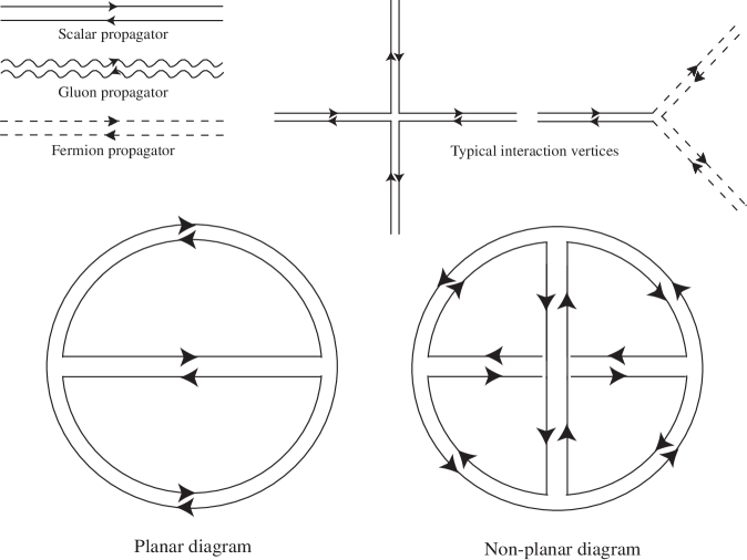
Figure 1: Typical Feynman rules for adjoint fields and sample planar and non-planar diagrams.

The vertices are drawn in a similar way, with directions of arrows indicating the fundamental or anti-fundamental indices of the generators. In this diagrammatic presentation, the propagators form the edges and the insides of loops are considered the faces. The one point compactification of the plane then means that the diagrams give rise to closed, compact and orientable surfaces, with Euler characteristic $\chi=V-P+F=2-2h$, where $h$ is the genus of the surface. The number of faces is one more than the number of loops, since the group theory always gives rise to an extra factor of $N$ for the last trace. In the simplical decomposition, with the one-point compactification, the outside of the diagram becomes another face, and can be interpreted as the last trace.

The perturbative expansion of the vacuum persistence amplitude takes the form of a double expansion

$$\sum_{h=0}^{\infty}N^{2-2h}P_{h}(\lambda)$$ (I.4)

with $h$ the genus and $P_{h}$ some polynomial in $\lambda$, which itself admits a power series expansion

$$P_{h}(\lambda)=\sum_{n=0}^{\infty}C_{h,n}\lambda^{n}$$ (I.5)

The simple idea is that all the diagrams generated for the vacuum correlation function can be grouped in classes based on their genera, and all the diagrams in each class will have varying dependences on the ’t Hooft coupling $\lambda$. Collecting together all the diagrams in a given class again into groups sharing the same dependence on $\lambda$, we can extract the $h$ and $n$ dependent constant $C_{h,n}$. It is clear from (I.4) that for large $N$, the dominant contributions come from diagrams of the lowest genus, the planar (or spherical) diagrams.

The double expansion (I.4) and (I.5) looks remarkably similar to the perturbative expansion for a string theory with coupling constant $1/N$ and with the expansion in powers of $\lambda$ playing the role of the worldsheet expansion. The analogy extends to the genus expansion, with the Feynman diagrams loosely forming a sort of discretized string worldsheet. At large $N$, such a string theory would be weakly coupled. The string coupling measures the difference in the Euler character for worldsheet diagrams of different topology. This has long suggested the existence of a duality between gauge and string theory. We of course also have to account for the mapping of non-perturbative effects on the two sides of the duality.

So far we have considered only the vacuum diagrams, though the same arguments go through when considering correlation functions with insertions of the fields. The action appearing in the generating functional of connected diagrams must be supplemented with terms coupling the fundamental fields to currents, and these terms will enter with a factor of $N$. The planar (leading) contributions to such correlation functions with $j$ insertions of the fields will be suppressed by an extra factor of $N^{-j}$ relative to the vacuum diagrams. The one particle irreducible three and four point functions then come with factors of $1/N$ and $1/N^{2}$ relative to the propagator, suggesting that $1/N$ is the correct expansion parameter. The expansion (I.4) for these more general correlation functions still holds if we account for the extra factors of $N$ coming from the insertions of the fields. The extra factor depends on the number of fields in the correlation function, but is fixed for the perturbative expansion of a given correlator.

The picture we have formed is of an oriented closed string theory. Adding matter in the fundamental representation would correspond to including propagators with a single line, and these could then form the edges of the worldsheets, and so would correspond to a dual theory with open strings (with the added possibility of D-branes). Generalizations to other gauge groups such as $O(N)$ and $Sp(N)$ would lead to unorientable worldsheets, since their adjoint representations (which are real) appear like products of fundamentals with fundamentals. This viewpoint has been applied to other types of theories, for example, non-linear sigma models with a large number of fundamental degrees of freedom.

The new ingredient relevant to our discussion will be the following: for a conformally invariant theory such as ${\cal N}=4$ SYM, the $\beta$ function vanishes for all values of the coupling $g_{YM}$ (it has a continuum of fixed points). There is no natural scale in this theory that should be held fixed. This makes limits different from the ’t Hooft limit possible, and we take advantage of such an opening via the so called BMN limit, which we discuss at length in what follows. Not all such limits are well-defined. In the BMN limit, we will consider operators with large numbers of fields. If the number of fields is scaled with $N$, generically, higher genus diagrams will dominate lower genus ones, and the genus expansion will break down. The novel feature of the BMN limit is that the combinatorics of these large numbers of fields conspire in a way that makes it possible for diagrams of all genera to contribute without the relative suppression typical in the ’t Hooft limit. In this sense, the BMN limit is the balancing point between two regions, one where the diagrams of higher genus are suppressed and don’t contribute in the limit, and the other where the limit is meaningless.

A concise introduction to the basic ideas underlying the large $N$ expansion can be found in ’t Hooft (2002), with a more detailed review presented in ’t Hooft (1994). Applications to QCD are given in Manohar (1998). A review of the large $N$ limit in field theories and the relation to string theory can also be found in Aharony et al. (2000), which discusses many issues related to $AdS$ spaces, conformal field theories and the celebrated $AdS/CFT$ correspondence.

I.2 String/gauge theory duality

’t Hooft’s original demonstration that the large $N$ limit of $U(N)$ gauge theory, as we have already discussed, is dual to a string theory, has sparked many attempts to construct such a duality explicitly. One such attempt Gross (1993); Gross and Taylor (1993) was to construct the dual to two-dimensional pure $QCD$ as a map from two-dimensional worldsheets of a given genus into a two-dimensional target space. $QCD_{2}$ is almost a topological theory, with the correlation functions depending only on the topology and area of the manifold on which the theory is formulated, making the theory exactly solvable. The partition function of this string theory sums over all branched coverings of the target space, and can be evaluated by discretizing the target using a two-dimensional simplical complex with an $N\times N$ matrix placed at each link. The partition function thus constructed can be evaluated exactly via an expansion in terms of group characters, giving rise to a matrix model, whose solution has been given in Kazakov et al. (1996); Kostov and Staudacher (1997); Kostov et al. (1998). Zero dimensional $QCD$ was considered in Brezin et al. (1978), as a toy model which retains all the diagrammatic but with trivial propagators, allowing the investigation of combinatorial counting in matrix models.

Another realization of ’t Hooft’s observation, this time via conventional string theory, is the celebrated AdS/CFT correspondence. The duality is suggested by the two viewpoints presented by D-branes. The low energy effective action of a stack of $N$ coincident D3-branes is given by ${\cal N}=4$ super-Yang-Mills theory with gauge group $U(N)$. While away from the brane the theory is type IIB closed string theory, there exists a decoupling limit where the closed strings of the bulk are decoupled from the gauge theory living on the brane Maldacena (1998). D3-branes are $1/2$ BPS, breaking $16$ of the supercharges of the type IIB vacuum, which in the decoupling limit will be non-linearly realized as the superconformal supercharges in the ${\cal N}=4$ worldvolume theory of the branes which exhibits superconformal invariance. For large $N$, the stack of D-branes will back-react, modifying the geometry seen by the type IIB strings. In the low energy description given by supergravity, the presence of the D-brane is seen in the form of the vacuum for the background fields like the metric and the Ramond-Ramond fields. These are two different descriptions of the physics of the stack of D-branes, and the ability to take these different viewpoints is the essence of the AdS/CFT duality according which type IIB superstring theory on the $AdS_{5}\times S^{5}$ background is dual to (or can be equivalently described by) ${\cal N}=4,\ D=4$ $U(N)$ supersymmetric Yang-Mills theory with a prescribed mapping between string theory and gauge theory objects.

The specific prescription for the correspondence is suggested by the matching of the global symmetry groups and their representations on the two sides of the duality. The matching extends to the partition function of the ${\cal N}=4$ SYM on the boundary of $AdS_{5}$ ($R\times S^{3}$) and the partition function of IIB string theory on $AdS_{5}\times S^{5}$ Witten (1998)

$$\Big{\langle}e^{\int d^{4}x\;\phi_{0}(x){\cal O}(x)}\Big{\rangle}_{\rm CFT}={\cal Z}_{string}\left[\phi|_{boundary}=\phi_{0}(x)\right]\ ,$$ (I.6)

where the left-hand-side is the generating function of correlation functions of gauge invariant operators ${\cal O}$ in the gauge theory (such correlation functions are obtained by taking derivatives with respect to $\phi_{0}$ and setting $\phi_{0}=0$) and the right-hand-side is the full partition function of (type IIB) string theory on the $AdS_{5}\times S^{5}$ background with the boundary condition that the field $\phi=\phi_{0}$ on the $AdS$ boundary Aharony et al. (2000). The dimensions of the operators ${\cal O}$ (i.e. the charge associated with the behavior of the operator under rigid coordinate scalings) correspond to the free-field masses of the bulk excitations. Every operator in the gauge theory can be put in one to one correspondence with a field propagating in the bulk of the $AdS$ space, e.g. the gauge invariant chiral primary operators and their descendents on the Yang-Mills side can be put in a one to one correspondence with the the supergravity modes of the type IIB theory. In the low energy approximation to the string theory, we have type IIB supergravity, with higher order $\alpha^{\prime}$ corrections from the massive string modes. (Note, however, that the $AdS_{5}\times S^{5}$  background itself is an exact solution to supergravity with all $\alpha^{\prime}$-corrections included.) The relation (I.2) between the radius of $AdS_{5}$ (and also $S^{5}$) shows that when the gauge theory is weakly coupled, the radius of $AdS_{5}$ is small in string units. In this regime, the supergravity approximation breaks down. Of course, to make the duality complete, we have to find the mapping for the non-perturbative objects and effects on the two sides of the duality.

This conjecture has been generalized and restated for string theories on many deformations of the $AdS_{5}\times S^{5}$ background, such as $AdS_{5}\times T^{1,1}$ Klebanov and Witten (1998), the orbifolds of $AdS_{5}\times S^{5}$ space Gukov (1998); Lawrence et al. (1998); Kachru and Silverstein (1998), and even non-conformal cases Klebanov and Strassler (2000); Polchinski and Strassler (2000) and $AdS_{3}\times S^{3}\times M_{4}$ Giveon et al. (1998); Kutasov and Seiberg (1999). For example in the Klebanov-Witten case, the statement is that type IIB strings on $AdS_{5}\times T^{1,1}$ background are the ’t Hooft strings of an ${\cal N}=1$ super-conformal field theory and for the $AdS_{3}\times S^{3}$ case, ’t Hooft strings of the ${\cal N}=(4,4)$ $D=2$ super-conformal field theory are dual to strings on $AdS_{3}\times S^{3}\times T^{4}$. The latter have been made explicit by the Kutasov-Seiberg construction Giveon et al. (1998); Kutasov and Seiberg (1999). In general it is a non-trivial task to determine the ’t Hooft string picture of a given gauge theory.

I.3 Moving away from supergravity limit, strings on plane-waves

Although Witten’s formula (I.6) is precise, from a practical point of view, our calculational ability does not go beyond the large $N$ limit which corresponds to the supergravity limit on the string theory side (except for quantities which are protected by supersymmetry, the calculations on both sides of the duality beyond the large $N$ limit exhibit the same level of difficulty). However, one may still hope to go beyond the supergravity limit which corresponds to restricting to some particular sector of the gauge theory.

In this section we recall some basic observations and facts which led BMN to their conjecture Berenstein et al. (2002b) as well as a brief summary of the results obtained based on and in support of the conjecture. These observations and results will be discussed in some detail in the main part of this review.

• Although so far we have not been able to solve the string $\sigma$-model in the $AdS_{5}\times S^{5}$ background and obtain the spectrum of (free) strings, the Penrose limit Penrose (1976); Gueven (2000) of $AdS_{5}\times S^{5}$ geometry results in another maximally supersymmetric background of type IIB which is the plane-wave geometry. The corresponding $\sigma$-model (in the light-cone gauge) is solvable, allowing us to deduce the spectrum of (free) strings on this plane-wave background.

• Taking the Penrose limit on the gravity side corresponds to restricting the gauge theory to operators with a large charge under one of its global symmetries (more precisely the R-symmetry charge associated with a $U(1)\subset SO(6)_{R}$) $J$, the BMN sector, and simultaneously taking the large $N$ limit.

• The BMN sector of ${\cal N}=4,\ D=4$ $U(N)$ SYM theory is comprised of operators with large conformal dimension $\Delta$ and large R-charge $J$, such that

  $$\frac{1}{\mu}p^{-} \equiv\Delta-J={\rm fixed}\,,$$ (I.7a)

  $$\alpha^{\prime}\mu p^{+} \equiv\frac{1}{2\sqrt{g^{2}_{YM}N}}(\Delta+J)={\rm fixed}\,,$$ (I.7b)

  together with

  $$g_{YM}={\rm fixed}\ ,\ \ \ \ \ \frac{J^{2}}{N}={\rm fixed},\ \ \ N\to\infty\ ,\ \ \ J\to\infty\ .$$ (I.8)

  In the above $\frac{1}{\mu}p^{-}$ and $\alpha^{\prime}\mu p^{+}$ are the corresponding string light-cone Hamiltonian and light-cone momentum, respectively. The parameter $\mu$ is a convenient but auxiliary parameter, the role of which will become clear in the following sections.

• In (I.7a), $p^{-}$ should be understood as the full plane-wave light-cone string (field) theory Hamiltonian. Explicitly, one can interpret (I.7a) as an equality between two operators, the plane-wave light-cone string field theory Hamiltonian, $H_{SFT}$, on one side and the difference between the dilatation and the R-charge operators on the other side, i.e.

  $$\frac{1}{\mu}H_{SFT}={\cal D}-{\cal J}\ ,$$ (I.9)

  where ${\cal D}$ is the dilatation operator and ${\cal J}$ is the R-charge generator. Therefore according to the identification (I.9) which is the (improved form of the original) BMN conjecture, the spectrum of strings, which are the eigenvalues of the light-cone Hamiltonian $p^{-}=H_{SFT}$, should be equal to the spectrum of the dialtation operator, which is the Hamiltonain of the ${\cal N}=4,$ gauge theory on $\mathbb{R}\times S^{3}$, restricted to the operators in the BMN sector of the gauge theory (defined through (I.7) and (I.8)).

• As stated above, equation (I.9) sets an equivalence between two operators. However, the second part of the BMN conjecture is about the correspondence between the Hilbert spaces that these operators act on; on the string theory side, it is the string (field) theory Hilbert space which is comprised of direct sum of the zero string, single string, double string and … string states, quite similarly to the flat space case Polchinski (1998a). On the gauge theory side it is the so-called BMN operators, the set of $U(N)$ invariant operators of large R-charge $J$ and large dimension in the free gauge theory, subject to (I.7) and (I.8).

• According to the BMN proposal Berenstein et al. (2002b), single string states map to certain single trace operators in the gauge theory. In particular, the single string vacuum state in the sector with light-cone momentum $p^{+}$, $(\alpha^{\prime}\mu p^{+})^{2}=\frac{J^{2}}{g^{2}_{YM}N}$, is identified with the chiral-primary BPS operator

  $$|0,p^{+}\rangle\longleftrightarrow{\cal N}_{J}{\rm Tr}(Z^{J})|vac\rangle\ ,$$ (I.10)

  where ${\cal N}_{J}$ is a normalization constant that will be fixed later in section VI. In the above, $Z=\frac{1}{\sqrt{2}}(\phi^{5}+i\phi^{6})$, where $\phi^{5}$ and $\phi^{6}$ are two of the six scalars of the ${\cal N}=4,\ D=4$ gauge multiplet. The R-charge we want to consider, $J$, is the eigenvalue for a $U(1)$ generator, $U(1)\subset SU(4)_{R}$, so that $Z$ carries unit charge and all the other bosonic modes in the vector multiplet, four scalars and four gauge fields, have zero R-charge. Since all scalars have $\Delta=1$ (classically), for $Z$ and hence $Z^{J}$, $\Delta-J=0$. The advantage of identifying string vacuum states with the chiral-primary operators is two-fold: i) they have $\frac{1}{\mu}p^{-}=\Delta-J=0$, and ii) their anomalous dimension is zero and hence the corresponding $p^{-}$ remains zero to all orders in the ’t Hooft coupling and even non-perturbatively, see for example D’Hoker and Freedman (2002).

• As for stringy excitations above the vacuum, BMN conjectured that we need to work with certain “almost” BPS operators, i.e. certain operators with large $J$ charge and with $\Delta-J\neq 0$, but $\Delta-J\ll J$. In particular, single closed string states were (originally) proposed to be dual to single trace operators with $\Delta-J=2$. The exact form of these operators and a more detailed discussion regarding them will be presented in section V. As we will see in sections VII.2.2 and VII.3, however, this identification of the single string Hilbert space with the single trace operators, because of the mixing between single trace and multi trace operators, should be modified. Note that this mixing is present both for chiral primaries and “almost” primaries.

• As is clear from (I.8), in the BMN limit the ’t Hooft coupling goes to infinity and naively any perturbative calculation in the gauge theory (of course except for chiral-primary two and three point functions) is not trustworthy. However, the fact that we are working with “almost” BPS operators motivates the hope that, although the anomalous dimensions for such operators are non-vanishing, being close to primary, nearly saturating the BPS bound, some of the nice properties of primary operators might be inherited by the “almost” primary operators.

• We will see in section VII, as a result of explicit gauge theory calculations with the BMN operators, that the ’t Hooft coupling in the BMN sector is dressed with powers of $1/J^{2}$. More explicitly, the effective coupling in the BMN sector is $\lambda^{\prime}$, rather than the ’t Hooft coupling $\lambda$, where

  $$\lambda^{\prime}\equiv\frac{\lambda}{J^{2}}=g^{2}_{YM}\frac{N}{J^{2}}=(\alpha^{\prime}\mu p^{+})^{-2}\,.$$ (I.11)

  The last equality is obtained using (I.7) and (I.8).

• Moreover, we will see that the ratio of non-planar to planar graphs is controlled by powers of the genus counting parameter

  $$g_{2}\equiv\frac{J^{2}}{N}=4\pi g_{s}(\alpha^{\prime}\mu p^{+})^{2}\,,$$ (I.12)

  which also remains finite in the BMN limit (I.8). Note that in (I.12) $g_{s}=e^{\phi}$, where $\phi$ is the value of the dilaton field, is not the coupling for strings on the plane-wave, although it is related to it.

• One can do better than simply finding the free string mass spectrum; we can study real interacting strings, their splitting and joining amplitudes and one loop corrections to the mass spectrum. As we will discuss in sections VII and VIII, the one-loop mass corrections compared to the tree level results are suppressed by powers of the “effective one-loop string coupling” (cf. (VII.34))

  $$g^{eff}_{one-loop}=\sqrt{\lambda^{\prime}g_{2}^{2}}=g_{YM}\frac{J}{\sqrt{N}}=4\pi g_{s}\ \alpha^{\prime}\mu p^{+}.$$ (I.13)

  It has been argued that all higher genus (higher loop) results replicate the same pattern, i.e. $g_{2}$ always appears in the combination $\lambda^{\prime}g_{2}^{2}$. This has been built into a quantum mechanical model for strings on plane-waves, the string bit model Vaman and Verlinde (2002); Verlinde (2002). However, a priori there is no reason why such a structure should exist and in principle $g_{2}$ and $\lambda^{\prime}$ can appear in any combination. Using another quantum mechanical model constructed to capture some features of the BMN operator dynamics, it has been argued that at $g_{2}^{4}$ level there are indeed $\lambda^{\prime}g_{2}^{4}$ corrections to the mass spectrum Beisert et al. (2003c); Plefka (2003).

• The above observations revive the hope that we might be able to do a full-fledged interacting string theory computation using perturbative gauge theory with (modified) BMN operators.

We should note that the BMN proposal has, since its inception, undergone many refinements and corrections. However, a full and complete understanding of the dictionary of strings on plane-waves and the (modified) BMN operators is not yet at our disposal, and the field is still dynamic. Some of the open issues will be discussed in the main text and in particular in section IX.

Finally, we would like to remind the reader that in this review we have tried to avoid many detailed and lengthy calculations, specifically in sections VI, VII and VIII. In fact, we found the original papers on these calculations quite clear and useful and for more details the reader is encouraged to consult with the references provided.

II Plane-waves as solutions of supergravity

Plane-fronted gravitational waves with parallel rays, pp-waves, are a general class of spacetimes and are defined as spacetimes which support a covariantly constant null Killing vector field $v^{\mu}$,

$$\nabla_{\mu}v_{\nu}\>=\>0\ ,\ \ \ \ \ \ v^{\mu}v_{\mu}\>=\>0\,.$$ (II.1)

In the most general form, they have metrics which can be written as

$$ds^{2}\>=\>-2dudv-F(u,x^{I})du^{2}+2A_{J}(u,x^{I})dudx^{J}+g_{JK}(u,x^{I})dx^{J}dx^{K}\,,$$ (II.2)

where $g_{JK}(u,x^{I})$ is the metric on the space transverse to a pair of light-cone directions given by $u,v$ and the coefficients $F(u,x^{I})$, $A_{J}(u,x^{I})$ and $g_{JK}(u,x^{I})$ are constrained by (super-)gravity equations of motion. The pp-wave metric (II.2) has a null Killing vector given by $\frac{\partial}{\partial v}$ which is in fact covariantly constant by virtue of the vanishing of the $\Gamma^{v}_{vu}$ component of the Christoffel symbol.

The most useful pp-waves, and the ones generally considered in the literature, have $A_{J}=0$ and are flat in the transverse directions, i.e. $g_{IJ}=\delta_{IJ}$, for which the metric becomes

$$ds^{2}\>=\>-2dudv-F(u,x^{I})du^{2}+\delta_{IJ}dx^{I}dx^{J}\ .$$ (II.3)

As we will discuss in the next subsection, existence of a covariantly constant null Killing vector field guarantees the $\alpha^{\prime}$-exactness of these supergravity solutions Horowitz and Steif (1990).

A more restricted class of pp-waves, plane-waves, are those admitting a globally defined covariantly constant null Killing vector field. One can show that for plane-waves $F(u,x^{I})$ is quadratic in the $x^{I}$ coordinates of the transverse space, but still can depend on the coordinate $u$, $F(u,x^{I})=f_{IJ}(u)x^{I}x^{J}$, so that the metric takes the form

$$ds^{2}\>=\>-2dudv-f_{IJ}(u)x^{I}x^{J}du^{2}+\delta_{IJ}dx^{I}dx^{J}\ .$$ (II.4)

Here $f_{IJ}$ is symmetric and by virtue of the only non-trivial condition coming form the equations of motion, its trace is related to the other field strengths present. For the case of vacuum Einstein equations, it is traceless.

There is yet a more restricted class of plane-waves, homogeneous plane-waves, for which $f_{IJ}(u)$ is a constant, hence their metric is of the form

$$ds^{2}\>=\>-2dudv-\mu^{2}_{IJ}x^{I}x^{J}du^{2}+dx^{I}dx^{I}\ ,$$ (II.5)

with $\mu^{2}_{IJ}$ being a constant.

II.1 Penrose diagrams for plane-waves

Penrose diagrams Penrose (1963) are useful tools which capture the causal structure of spacetimes. The idea is based on the observation that metrics which are conformally equivalent share the same light-like geodesics, and hence such spacetimes have the same causal structure (for a more detailed discussion see Townsend (1997)). Generically, if there is enough symmetry, it is possible to bring a given metric into a conformally flat form or to the form conformal to Einstein static universe (a $d+1$ dimensional cylinder with the metric $ds^{2}=-dt^{2}+d\Omega^{2}_{d}$), where usually coordinates have a finite range. One can then use this coordinate system to draw Penrose diagrams. Therefore, Penrose diagrams are constructed so that the light rays always move on $45^{\circ}$ lines Misner et al. (1970) and in which one can visualize the whole causal structure, singularities, horizons and boundaries of spacetimes. It may happen that a given coordinate system does not cover the entire spacetime, or it may be possible to (analytically) extend them. A Penrose diagram is a very useful way to see if there is a possibility of extending the spacetime and provides us with a specific prescription for doing so. In the conformally flat coordinates (or coordinate system in which the metric is Einstein static universe up to a conformal factor) all the information characterizing the spacetime is embedded in the conformal factor. It may happen that, within the range of the coordinates, this conformal factor is regular and finite. In such cases we can simply extend the range of coordinates to the largest possible range. However, if the conformal factor blows up (or vanishes), we have a boundary or singularity. For example in a $d+1$ dimensional flat space, the conformal factor blows up and hence we have a ($d$ dimensional) light-like boundary with no possibility for further extension Misner et al. (1970).

Let us consider the plane-waves and analyze their Penrose diagrams. Since in this review we will only be interested in a special homogeneous plane-wave of the form (II.5) with $\mu^{2}_{IJ}=\mu^{2}\delta_{IJ},\ I,J=1,2,\cdots,d-1$, we will narrow our focus to this special case. First we note that with the coordinate transformation Berenstein and Nastase (2002)

$$y^{0}=\frac{1}{2\mu}(1+\mu^{2}x^{2})\tan\mu u+v\ ,\ \ y^{d}=\frac{1}{2\mu}(1-\mu^{2}x^{2})\tan\mu u-v\ ,\ \ y^{I}=\frac{x^{I}}{\cos\mu u}\ ,$$ (II.6)

the metric becomes

$$ds^{2}=\frac{1}{1+\mu^{2}(y^{0}+y^{D})^{2}}(\eta_{\check{\alpha}\check{\beta}}dy^{\check{\alpha}}dy^{\check{\beta}})\ ,$$ (II.7)

where $\check{\alpha},\check{\beta}=0,1,\cdots,d$ and $\eta_{\check{\alpha}\check{\beta}}=diag(-,+,\cdots,+)$. Note that $y^{+}\equiv y^{0}+y^{d}\in(-\frac{\pi}{2\mu},\frac{\pi}{2\mu})$. To study the possibility of analytic extension of the spacetime, particularly over the range of $y^{+}$, and to draw the Penrose diagram, we make another coordinate transformation

$$r^{2}=y_{i}y_{i}\ ,\ \ i=1,\cdots,d\ ,\ \ \ \ y^{d}=r\cos\theta\,,$$ (II.8a)

$$y^{0}\pm r =\frac{1}{\mu}\tan\frac{\psi\pm\xi}{2}\ ,\ \ \ \ \psi,\xi,\theta\in[0,\pi]\ ,$$ (II.8b)

in which all the coordinates have a finite range. In these coordinates (II.7) is conformal to Einstein static universe

$$ds^{2}=\frac{1}{\mu^{2}}\frac{1}{(\cos\psi+\cos\xi)^{2}+(\sin\psi+\sin\xi\cos\theta)^{2}}[-d\psi^{2}+d\xi^{2}+\sin^{2}\xi^{2}d\Omega^{2}_{d-1}]\,.$$ (II.9)

To simplify the conformal factor we perform another coordinate transformation

$$-\tan\alpha\sin\beta=\cot\theta,\ \ \ \ -\sin\alpha\cos\beta=\cos\xi,\ \ \ \ \alpha\in[0,\frac{\pi}{2}],\ \beta\in[0,2\pi]\ ,$$

yielding

$$ds^{2}=\frac{1}{\mu^{2}}\frac{1}{|e^{i\psi}-\sin\alpha e^{i\beta}|^{2}}\left(-d\psi^{2}+d\alpha^{2}+\sin^{2}\alpha d\beta^{2}+\cos^{2}\alpha d\Omega^{2}_{d-2}\right)\,.$$ (II.10)

The metric (II.10) is conformal to the Einstein space $-d\psi^{2}+d\Omega^{2}_{d}$ and we have already made all the possible analytic extensions (after relaxing the range of $\psi$). This manifold, however, does not cover the whole Einstein manifold, because the conformal factor vanishes at (and only at) $\alpha=\frac{\pi}{2},\ \psi=\beta$, and this light-like direction is not part of the analytically continued plane-wave spacetime. Note that at $\alpha=\frac{\pi}{2}$ the $d-2$ sphere shrinks to zero and the metric essentially reduces to the $\psi,\beta$ plane.

The boundary of a spacetime is a locus which does not belong to the spacetime but is in causal contact with the points in the bulk of the spacetime; we can send and receive light rays from the bulk to the boundary in a finite time. It is straightforward to see that in fact the light-like direction $\alpha=\frac{\pi}{2},\ \psi=\beta$ is the boundary of the analytically continued plane-wave geometry.

In sum, we have shown that the plane-wave has a one dimensional light-like boundary. All the information about the (analytically continued) plane-wave geometry has been depicted in the Penrose diagram FIG. 2.

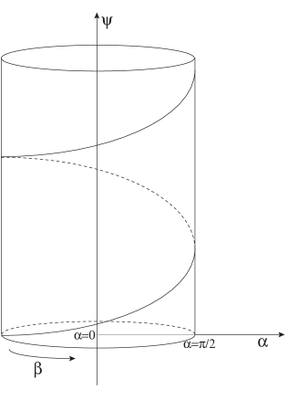
Figure 2: Penrose diagram of the plane-wave. The analytically continued plane-wave fills the whole Einstein static universe except for the light-like direction $\alpha=\frac{\pi}{2},\ \psi=\beta$, which is its boundary. Note that at each point (except for $\alpha=\frac{\pi}{2}$) there is an $S^{d-2}$ of finite radius, which is suppressed in the figure.

In the metric (II.10), we have chosen our coordinate system so that the entire $\mu$-dependence is gathered in an overall $1/\mu^{2}$ factor. Although in the original coordinate system the plane-wave metric has a smooth $\mu\to 0$ limit (which is flat space), for the analytically continued version (II.10) this is no longer the case. The reason is that some of our analytic extensions do not have a smooth $\mu\to 0$ limit. In particular, note that our arguments about boundary and causal structure of the plane-wave cannot be smoothly extended to the $\mu=0$ case. Finally we would like to note that the technique detailed here cannot be directly applied to a generic plane or pp-wave of the form (II.3). For these cases one needs to use the method of “Ideal asymptotic Points”, due to Geroch, Kronheimer and Penrose Geroch et al. (1972), application of which to pp-waves can be found in Hubeny and Rangamani (2002a); Marolf and Ross (2002).

II.2 Plane-waves as $\alpha^{\prime}$-exact solutions of supergravity

In this subsection we discuss a property of pp-waves of the form (II.3) which makes them specially interesting from the string theory point of view: they are $\alpha^{\prime}$-exact solutions of supergravity Horowitz and Steif (1990); Amati and Klimcik (1988). Supergravities arise as low energy effective theories of strings, and can receive $\alpha^{\prime}$-corrections. Such corrections generically involve higher powers of curvature and form fields Green et al. (1987a). The basic observation made by G. Horowitz and A. Steif Horowitz and Steif (1990) is that pp-wave metrics of the form (II.3) have a covariantly constant null Killing vector, $n_{\mu}=\frac{\partial}{\partial v}$, and their curvature is null (the only non-zero components of their curvature are $R_{uIuJ}$). Higher $\alpha^{\prime}$-corrections to the supergravity equations of motion are in general comprised of all second rank tensors constructed from powers of the Riemann tensor and its derivatives. (The only possible term involving only one Riemann tensor should be of the form $R^{\mu\alpha\nu\beta}_{\ \ \ \ \ \ ;\mu\nu}$, which is zero by virtue of the Bianchi identity.) On the other hand, any power of the Riemann tensor and its covariant derivatives with only two free indices is also zero, because $n_{\mu}$ is null and $\nabla_{\mu}n_{\nu}=0$ (II.1). The same argument can be repeated for the form fields, noting that for pp-waves which are solutions of supergravity these form fields should have zero divergence and be null. As a result, all the $\alpha^{\prime}$-corrections for supergravity solutions with metric of the form (II.3) vanish, i.e. they also solve $\alpha^{\prime}$-corrected supergravity equations of motion. This argument about $\alpha^{\prime}$-exactness does not hold for a generic pp-wave of the form (II.2) with $g_{IJ}(u,x^{I})\neq\delta_{IJ}$. The transverse metric, $g_{IJ}$, may itself receive $\alpha^{\prime}$-corrections, however, there are no extra corrections due to the wave part of the metric Fabinger and Hellerman (2003).We would like to comment that pp-waves are generically singular solutions with no (event) horizons Hubeny and Rangamani (2002b), however, plane-waves of the form (II.4) for which $f_{IJ}(u)$ is a smooth function of $u$, are not singular.

II.3 Maximally supersymmetric plane-wave and its symmetries

Hereafter in this review we shall only focus on a very special plane-wave solution of ten dimensional type IIB supergravity which admits 32 supersymmetries and by “the plane-wave” we will mean this maximally supersymmetric solution. In fact, demanding a solution of 10 or eleven dimensional supergravity to be maximally supersymmetric  is very restrictive; flat space, $AdS_{5}\times S^{5}$ and a special plane-wave in type IIB theory in ten dimensions and flat space, $AdS_{4,7}\times S^{7,4}$ and a special plane-wave in eleven dimensions are the only possibilities Figueroa-O’Farrill and Papadopoulos (2003). Note that type IIA does not admit any maximally supersymmetric solutions other than flat space.

Here, we only focus on the ten dimensional plane-wave which is a special case of (II.5) with $\mu^{2}_{IJ}=\mu^{2}\delta_{IJ}$. This metric, however, is not a solution to source-free type IIB supergravity equations of motion and we need to add form fluxes. It is not hard to see that with $\mu^{2}_{IJ}=\mu^{2}\delta_{IJ}$ the only possibility is turning on a constant self-dual RR five-form flux; moreover, the dilaton should also be a constant. As we will see in section III, this plane-wave is closely related to the $AdS_{5}\times S^{5}$ solution. The (bosonic) part of this plane-wave solution is then

$$ds^{2}=-2dx^{+}dx^{-}-\mu^{2}(x^{i}x^{i}+ x^{a}x^{a}){(dx^{+})}^{2}+dx^{i}dx^{i}+dx^{a}dx^{a},$$ (II.11a)

$$F_{+ijkl}=\frac{4}{g_{s}}\mu\ \epsilon_{ijkl}\ ,\ \ \ \ \ \ F_{+abcd}=\frac{4}{g_{s}}\mu\ \epsilon_{abcd}\ ,$$ (II.11b)

$$e^{\phi}=g_{s}={\rm constant}\ ,\ \ i,j =1,2,3,4\ ,\ \ a,b=5,6,7,8\ ,\ \$$ (II.11c)

In the above, $\mu$ is an auxiliary but convenient parameter, and can be easily removed by taking $x^{+}\to x^{+}/\mu$ and $x^{-}\to\mu x^{-}$ (which is in fact a light-cone boost).

Let us first check that the background (II.11) is really maximally supersymmetric. Note that this will ensure it is also a supergravity solution, because supergravity equations of motion are nothing but the commutators of the supersymmetry variations. For this we need to show that the gravitino and dilatino variations vanish for 32 independent (Killing) spinors, i.e.

$$\delta_{\epsilon}\psi^{\alpha}_{\mu}\equiv(\hat{\cal D}_{\mu})^{\alpha}_{\ \beta}\ \epsilon^{\beta}=0\ ,\ \ \ \delta_{\epsilon}\lambda^{\alpha}\equiv(\tilde{\cal D})^{\alpha}_{\ \beta}\ \epsilon^{\beta}=0\ ,\ \mu=0,1,\cdots,9,\ \alpha=1,2\ ,$$ (II.12)

have 32 solutions, where the dilatino $\lambda^{\alpha}$, gravitinos $\psi_{\mu}^{\alpha}$ and Killing spinors $\epsilon^{\alpha}$ are all 32 component ten dimensional Weyl-Majorana fermions of the same chirality (for our notations and conventions see Appendix B.1), and the supercovariant derivative $\hat{\cal D}_{\mu}$ in string frame is defined as (see for example Cvetic et al. (2003); Bena and Roiban (2003); Sadri and Sheikh-Jabbari (2003))

$$(\hat{{\cal D}}_{\mu})^{\alpha}_{\ \beta}=\delta^{\alpha}_{\ \beta}\ \nabla_{\mu}+\frac{1}{8}(\sigma^{3})^{\alpha}_{\ \beta}\ \Gamma^{\nu\rho}H_{\mu\nu\rho}+\frac{ie^{\phi}}{8}\left[(\sigma^{2})^{\alpha}_{\ \beta}\ \Gamma^{\nu}\partial_{\nu}\chi-\frac{i}{3!}(\sigma^{1})^{\alpha}_{\ \beta}\ \Gamma^{\nu\rho\lambda}F_{\nu\rho\lambda}+\frac{1}{2\cdot 5!}(\sigma^{2})^{\alpha}_{\ \beta}\ \Gamma^{\nu\rho\lambda\sigma\delta}F_{\nu\rho\lambda\sigma\delta}\right]\Gamma_{\mu},$$ (II.13)

$$(\tilde{\cal D})^{\alpha}_{\ \beta}=\frac{1}{2}\delta^{\alpha}_{\ \beta}\ \Gamma^{\nu}\partial_{\nu}\phi-\frac{1}{4\cdot 3!}(\sigma^{3})^{\alpha}_{\ \beta}\ \Gamma^{\mu\nu\rho}H_{\mu\nu\rho}-\frac{i}{2}e^{\phi}\left[(\sigma^{2})^{\alpha}_{\ \beta}\ \Gamma^{\nu}\partial_{\nu}\chi-\frac{i}{2\cdot 3!}(\sigma^{1})^{\alpha}_{\ \beta}\ \Gamma^{\nu\rho\lambda}F_{\nu\rho\lambda}\right]\ ,$$ (II.14)

with the spin connection $\omega_{\mu}^{\hat{a}\hat{b}}$ appearing in the covariant derivative $\nabla_{\mu}=(\partial_{\mu}+\frac{1}{4}\omega_{\mu}^{\hat{a}\hat{b}}\Gamma_{\hat{a}\hat{b}})$ and the hatted Latin indices used for the tangent space. In these expressions $\phi$ is the dilaton, $\chi$ the axion, $H$ the three-form field strength of the NSNS sector, and the $F$’s represent the appropriate RR field strengths.

For the background (II.11) $(\tilde{\cal D})^{\alpha}_{\ \beta}$ is identically zero and $(\hat{\cal D})^{\alpha}_{\ \beta}$ take a simple form

$$(\hat{{\cal D}}_{\mu})^{\alpha}_{\ \beta}=\delta^{\alpha}_{\ \beta}\ (\partial_{\mu}+\frac{1}{4}\omega_{\mu}^{ab}\Gamma_{ab})+\frac{ig_{s}}{16\cdot 5!}(\sigma^{2})^{\alpha}_{\ \beta}\ \Gamma^{\nu\rho\lambda\sigma\delta}F_{\nu\rho\lambda\sigma\delta}\ .$$ (II.15)

In order to work out the spin connection $\omega_{\mu}^{\hat{a}\hat{b}}$ we need the vierbeins $e_{\mu}^{\hat{a}}$ which are

$$e_{+}^{\ +}=e_{-}^{\ -}=1\ ,\ e_{i}^{\ j}=\delta_{i}^{\ j}\ ,e_{{a}}^{\ {b}}=\delta_{a}^{\ b}\ ,\ e_{+}^{\ -}=\frac{1}{2}\mu^{2}(x_{i}x_{i}+x_{a}x_{a})\ ,$$ (II.16)

and therefore

$$\omega_{+}^{\ -i}=\mu^{2}x_{i}\ ,\ \omega_{+}^{\ -a}=\mu^{2}x_{a}\ ,\$$ (II.17)

are the only non-vanishing components of $\omega_{\mu}^{\hat{a}\hat{b}}$.

The Killing spinor equation can now be written as

$$({\bf 1}\cdot\partial_{\mu}+\Omega_{\mu})^{\alpha}_{\ \beta}\ \epsilon^{\beta}=0\,,$$ (II.18)

with

$$\Omega_{-}=0\,,\ \ (\Omega_{I})^{\alpha}_{\ \beta}=\frac{i\mu}{4}\Gamma^{+}(\Pi+\Pi^{\prime})\Gamma^{I}(\sigma^{2})^{\alpha}_{\ \beta}\,,\ \ (\Omega_{+})^{\alpha}_{\ \beta}=-\frac{1}{2}\mu^{2}x^{I}\Gamma^{+I}\ \delta^{\alpha}_{\ \beta}+\frac{i\mu}{4}(\Pi+\Pi^{\prime})\Gamma^{+}\Gamma_{+}\ (\sigma^{2})^{\alpha}_{\ \beta}\,.$$ (II.19)

In the above $I=\{i,a\}=1,2,\cdots 8,\ \Pi=\Gamma^{1234}$ and $\Pi^{\prime}=\Gamma^{5678}$. The $\Omega$’s satisfy a number of useful identities such as

$$\Gamma^{+}\Omega_{I}=\Omega_{I}\Gamma^{+}=\Gamma^{+}\Omega_{+}=0\ \ \ \Omega_{I}\Omega_{J}=\Omega_{I}\Omega_{+}=0\ ,$$ , (II.20)

$$\Omega_{+}\Omega_{I}=-\frac{\mu^{2}}{4}(1+\Pi\Pi^{\prime})\Gamma^{+I}\cdot{\bf 1}\ \ \ \Omega_{+}\Gamma^{+}=\frac{i\mu}{2}(\Pi+\Pi^{\prime})\Gamma^{+}\cdot{(\sigma^{2})^{\alpha}_{\ \beta}}\ .$$ , (II.21)

We first note that the ($\mu=-$) component of (II.18) is simply $\partial_{-}\epsilon=0$, so all Killing spinors should be $x^{-}$-independent. The $\mu=I$ component can be easily solved by taking

$$\epsilon^{\alpha}=({\bf 1}-x^{I}{\Omega_{I}})^{\alpha}_{\ \beta}\chi^{\beta}\,,$$ (II.22)

where $\chi^{\beta}$ is an arbitrary $x^{I}$-independent fermion of positive ten dimensional chirality. Plugging (II.22) into (II.18), using the identity $\Omega_{I}\Omega_{+}=0$ and the fact that $({\bf 1}+x^{I}{\Omega_{I}})({\bf 1}-x^{I}{\Omega_{I}})={\bf 1}$ the ($\mu=+$) component of the Killing spinor equation takes the form

$$\left({\bf 1}\cdot\partial_{+}+\Omega_{+}({\bf 1}-x^{I}\Omega_{I})\right)^{\alpha}_{\ \beta}\chi^{\beta}=0\ .$$ (II.23)

Equation (II.23) has an $x^{I}$ independent piece and a part which is linear in $x^{I}$. These two should vanish separately. Using the identities given in Appendix B.1 and after some straightforward Dirac matrix algebra, one can show that if $\Gamma^{-}\chi=0$, (II.23) simply reduces to $\partial_{+}\chi=0$. That is, any constant $\chi$ with $\Gamma^{-}\chi=0$ is a Killing spinor. These provide us with $2\times 8=16$ solutions. Now let us assume that $\Gamma^{-}\chi\neq 0$. Without loss of generality, all such spinors can be chosen to satisfy $\Gamma^{+}\chi=0$. For these choices of $\chi$’s the $x^{I}$-dependent part of (II.23) vanishes identically and the $x^{I}$-independent part becomes

$$\left({\bf 1}\cdot\partial_{+}+{i\mu}\Pi\ (\sigma^{2})^{\alpha}_{\ \beta}\right)\chi^{\beta}=0\,,$$

where we have used the fact that $\Gamma^{+}\chi=0$ implies $\Pi\chi=\Pi^{\prime}\chi$. This equation can be easily solved with Blau et al. (2002a)

$$\chi^{\alpha}=\left(\delta^{\alpha}_{\ \beta}\ \cos{\mu x^{+}}-i\Pi\ (\sigma^{2})^{\alpha}_{\ \beta}\ \sin{\mu x^{+}}\right)\chi_{0}^{\beta}\ ,$$ (II.24)

where $\chi_{0}^{\beta}$ is an arbitrary constant spinor of positive ten dimensional chirality. We have shown that equations (II.12) have 32 linearly independent solutions and hence the background (II.11) is maximally supersymmetric. We would like to note that (II.24) clearly shows the “wave” nature of our background (note the periodicity in $x^{+}$, the light-cone time), a fact which is not manifest in the coordinates we have chosen. This wave nature can be made explicit in the so-called Rosen coordinates (cf. section III.1).

II.3.1 Isometries of the background

The background (II.11) has a number of isometries, some of which are manifest. In particular, the solution is invariant under translations in the $x^{+}$ and $x^{-}$ directions. These translations can be thought of as two (non-compact) $U(1)$’s with the generators

$$i\frac{\partial}{\partial x^{+}}\equiv P_{+}=-P^{-}\ ,\ \ \ i\frac{\partial}{\partial x^{-}}\equiv P_{-}=-P^{+}\ .$$ (II.25)

Due to the presence of the $(dx^{+})^{2}$ term, a boost in the ($x^{+},x^{-}$) plane is not a symmetry of the metric. However, the combined boost and $\mu$ scaling:

$$x^{-}\to\sqrt{\frac{1-v}{1+v}}x^{-}\ ,\ \ x^{+}\to\sqrt{\frac{1+v}{1-v}}x^{+}\ ,\ \ \mu\to\sqrt{\frac{1-v}{1+v}}\mu\ ,$$ (II.26)

is still a symmetry.

Obviously, the solution is also invariant under two $SO(4)$’s which act on the $x^{i}$ and $x^{a}$ directions. The generators of these $SO(4)$’s will be denoted by $J_{ij}$ and $J_{ab}$ where

$$J_{ij}=-i(x_{i}\frac{\partial}{\partial x^{j}}-x_{j}\frac{\partial}{\partial x^{i}})\ ,\ \ \ J_{ab}=-i(x_{a}\frac{\partial}{\partial x^{b}}-x_{b}\frac{\partial}{\partial x^{a}})\ .$$ (II.27)

Note that although the metric possesses $SO(8)$ symmetry, because of the five-form flux this symmetry is broken to $SO(4)\times SO(4)$. There is also a $\mathbb{Z}_{2}$ symmetry which exchanges these two $SO(4)$’s, acting as

$$\{x^{i}\}{\overset{\mathbb{Z}_{2}}{\longleftrightarrow}}\{x^{a}\}\ .$$ (II.28)

So far we have identified 14 isometries which are generators of a $U(1)\times U(1)\times SO(4)\times SO(4)\rtimes\mathbb{Z}_{2}$ symmetry group. One can easily see that translations along the $x^{I}=(x^{i},\ x^{a})$ directions are not symmetries of the metric. However, we can show that if along with translation in $x^{I}$ we also shift $x^{-}$ appropriately, i.e.

$$\left\{\begin{array}[]{cc}x^{I}\to x^{I}+\epsilon_{1}^{I}\ \cos\mu x^{+}\cr x^{-}\to x^{-}-\epsilon_{1}^{I}\ \mu x^{I}\sin\mu x^{+}\end{array}\right.\ ,\ \ \ \ \ \left\{\begin{array}[]{cc}x^{I}\to x^{I}+\epsilon_{2}^{I}\ \sin\mu x^{+}\cr x^{-}\to x^{-}+\epsilon_{2}^{I}\ \mu x^{I}\cos\mu x^{+}\end{array}\right.\ ,$$ (II.29)

where $\epsilon_{1}^{I}$ and $\epsilon_{2}^{I}$ are arbitrary but small parameters, the metric and the five-form remain unchanged. These 16 isometries are generated by the Killing vectors

$$L_{I}=-i\left(\cos\mu x^{+}\frac{\partial}{\partial x^{I}}-\mu x^{I}\ \sin\mu x^{+}\frac{\partial}{\partial x^{-}}\right)\ ,\ \ \ K_{I}=-i\left(\sin\mu x^{+}\frac{\partial}{\partial x^{I}}+\mu x^{I}\ \cos\mu x^{+}\frac{\partial}{\partial x^{-}}\right)\ ,$$ (II.30)

satisfying the following algebra

$$[L_{I},L_{J}]=0\ ,\ \ \ \ [L_{I},K_{J}]=\mu\delta_{IJ}\frac{\partial}{\partial x^{-}}=i\mu P^{+}\ \delta_{IJ}\ ,\ \ \ \ [K_{I},K_{J}]=0\ ,$$ (II.31)

$$[P^{-},L_{I}]=i\mu\ K_{I}\ ,\ \ \ \ [P^{-},K_{I}]=-i\mu\ L_{I}\ .$$ (II.32)

Equations (II.31) are in fact an eight (or a pair of four) dimensional Heisenberg-type algebra(s) with “$\hbar$” being equal to $\mu P^{+}$ Das et al. (2002). Note that $P^{+}$ commutes with the generators of the two $SO(4)$’s as well as $K_{I}$ and $L_{I}$. In other words $P^{+}$ is in the center of the isometry algebra which has 30 generators $(J_{ij},\ J_{ab},\ P^{+},\ P^{-},\ K_{i},\ K_{a},\ L_{i},\ L_{a})$. It is also easy to check that $K_{i},\ L_{j}$ and $K_{a},\ L_{b}$ transform as vectors (or singlets) under the corresponding $SO(4)$ rotations. Altogether, the algebra of Killing vectors is $[h(4)\oplus h(4)]\oplus so(4)\oplus so(4)\oplus u(1)_{+}\oplus u(1)_{-}$, where $h(4)$ is the four dimensional Heisenberg algebra.

In addition to the above 30 Killing vectors generating continuous symmetries, there are some discrete symmetries, one of which is the $\mathbb{Z}_{2}$ discussed earlier. There is also the CPT symmetry Schwarz (2002)

$$x^{I}\to-x^{I}\ ,\ \ \ \ \ x^{\pm}\to\ -x^{\pm}\ ,\ \ \ \ \ \ \mu\to\ -\mu\ ,$$ (II.33)

(note that we also need to change $\mu$).

Finally, it is useful to compare the plane-wave isometries to that of flat space, the ten dimensional Poincare algebra consisting of $P^{+},\ P^{-},\ P^{I}=-i\frac{\partial}{\partial x^{I}}$ and $J^{+-}$ (light-cone boost), $J^{+I},\ J^{-I}$ and $J^{IJ}$ (the $SO(8)$ rotations). Among these 55 generators, $P^{+},\ P^{-}$ and $J^{ij},\ J^{ab}$ are also present in the set of plane-wave isometries. However, as we have discussed, $J^{+-}$ and $J^{-I}$ are absent. As for rotations generated by $J^{ia}$, only a particular rotation, namely the $\mathbb{Z}_{2}$ defined in (II.28), is present. From (II.30) it is readily seen that $K_{I}$ and $L_{I}$ are a linear combination of $P_{I}$ and $J^{+I}$,

$$P_{I}=-i\frac{\partial}{\partial x^{I}}\ ,\ \ \ J^{+I}=x^{+}P^{I}-x^{I}P^{+}\ ,$$ (II.34)

and it is easy to show that $[P^{-},J^{+I}]=-iP^{I}\ ,\ [P^{I},J^{+J}]=-i\delta_{IJ}P^{+}$. In summary, $J^{+-},\ J^{-I}$ and $J^{ia}$ (which are altogether 25 generators) are not present among the Killing vectors of the plane-wave and therefore the number of isometries of the plane-wave is $55-25=30$, agreeing with our earlier results.

II.3.2 Superalgebra of the background

As we have shown, the plane-wave background (II.11) possesses 32 Killing spinors and in section II.3.1 we worked out all the isometries of the background. In this subsection we combine these two results and present the superalgebra of the plane-wave geometry (II.11). Noting the Killing spinor equations and its solutions it is straightforward to work out the supercharges and their superalgebra (e.g. see Green et al. (1987a)).

As discussed earlier, the solutions to the Killing spinor equations are all $x^{-}$-independent. This implies that supercharges should commute with $P^{+}$. However, as discussed in II.3.1, $P^{+}$ commutes with all the bosonic isometries, and so is in the center of the whole superalgebra. Then, we noted that Killing spinors fall into two classes, either $\Gamma^{+}\chi=0$ or $\Gamma^{-}\chi=0$. The former lead to kinematical supercharges, $Q^{+\alpha}$ with the property that $\Gamma^{+}Q^{+\alpha}=0$, while the latter lead to dynamical supercharges $Q^{-\alpha}$, which satisfy $\Gamma^{-}Q^{-\alpha}=0$. Since both sets of dynamical and kinematical supercharges have the same (positive) ten dimensional chirality, the $Q^{+\alpha}$ are in the ${\bf 8_{s}}$ and $Q^{-\alpha}$ in the ${\bf 8_{c}}$ representation of the $SO(8)$ fermions (for details of the conventions see Appendix B.1).

For the plane-wave background, however, it is more convenient to use the $SO(4)\times SO(4)$ decomposition instead of $SO(8)$. The relation between these two has been worked out and summarized in Appendix B.2. We will use $q_{\alpha\beta}$ and $q_{\dot{\alpha}\dot{\beta}}$ for the kinematical supercharges and $Q_{\dot{\alpha}\beta}$ and $Q_{\alpha\dot{\beta}}$ for the dynamical ones. Note that all $q$ and $Q$ are complex fermions.

The superalgebra in the $SO(8)$ basis can be found in Blau et al. (2002b); Metsaev (2002). Here we present it in the $SO(4)\times SO(4)$ basis:

• Commutators of bosonic generators with kinematical supercharges:

$$[J^{ij},q_{\alpha\beta}]=\frac{1}{2}\ (i\sigma^{ij})_{\alpha}^{\ \rho}\ q_{\rho\beta}\ \ \ [J^{ij},q_{\dot{\alpha}\dot{\beta}}]=\frac{1}{2}\ (i\sigma^{ij})_{\dot{\alpha}}^{\ \dot{\rho}}\ q_{\dot{\rho}\dot{\beta}}\ ,$$ , (II.35)

$$[J^{ab},q_{\alpha\beta}]=\frac{1}{2}\ (i\sigma^{ab})_{\beta}^{\ \rho}\ q_{\alpha\rho}\ \ \ [J^{ab},q_{\dot{\alpha}\dot{\beta}}]=\frac{1}{2}\ (i\sigma^{ab})_{\dot{\beta}}^{\ \dot{\rho}}\ q_{\dot{\alpha}\dot{\rho}}\ ,\$$ , (II.36)

$$[K^{I},q_{\alpha\beta}]=[L^{I},q_{\alpha\beta}]=0\ ,\ \ [K^{I},q_{\dot{\alpha}\dot{\beta}}]=[L^{I},q_{\dot{\alpha}\dot{\beta}}]=0\ ,\ \$$ (II.37)

$$[P^{+},q_{\alpha\beta}]=[P^{+},q_{\dot{\alpha}\dot{\beta}}]=0\ ,\ \$$ (II.38)

$$[P^{-},q_{\alpha\beta}]=+i\mu q_{\alpha\beta}\ ,\ \ [P^{-},q_{\dot{\alpha}\dot{\beta}}]=-i\mu q_{\dot{\alpha}\dot{\beta}}\ .$$ (II.39)

• Commutators of bosonic generators with dynamical supercharges:

$$[J^{ij},Q_{\alpha\dot{\beta}}]=\frac{1}{2}\ (i\sigma^{ij})_{\alpha}^{\ \rho}\ Q_{\rho\dot{\beta}}\ \ \ [J^{ij},Q_{\dot{\alpha}\beta}]=\frac{1}{2}\ (i\sigma^{ij})_{\dot{\alpha}}^{\ \dot{\rho}}\ Q_{\dot{\rho}\beta}\ ,$$ , (II.40)

$$[J^{ab},Q_{\dot{\alpha}\beta}]=\frac{1}{2}\ (i\sigma^{ab})_{\beta}^{\ \rho}\ Q_{\dot{\alpha}\rho}\ \ \ [J^{ab},Q_{\alpha\dot{\beta}}]=\frac{1}{2}\ (i\sigma^{ab})_{\dot{\beta}}^{\ \dot{\rho}}\ Q_{\alpha\dot{\rho}}\ ,\$$ , (II.41)

$$[K^{i},Q_{\alpha\dot{\beta}}]=\frac{\mu}{2}\ (\sigma^{i})_{\alpha}^{\ \dot{\rho}}q_{\dot{\rho}\dot{\beta}} \ \ \ [K^{a},Q_{\alpha\dot{\beta}}]=-\frac{\mu}{2}\ (\sigma^{a})_{\dot{\beta}}^{\ \rho}q_{\alpha\rho}\ ,$$ , (II.42)

$$[K^{i},Q_{\dot{\alpha}\beta}]=\frac{\mu}{2}\ (\sigma^{i})_{\dot{\alpha}}^{\ \rho}q_{\rho\beta}\ \ \ \ [K^{a},Q_{\dot{\alpha}\beta}]=\frac{\mu}{2}\ (\sigma^{a})_{\beta}^{\ \dot{\rho}}q_{\dot{\alpha}\dot{\rho}}\ ,$$ , (II.43)

$$[L^{i},Q_{\alpha\dot{\beta}}]=-\frac{\mu}{2}\ (\sigma^{i})_{\alpha}^{\ \dot{\rho}}q_{\dot{\rho}\dot{\beta}}\ \ \ [L^{a},Q_{\alpha\dot{\beta}}]=\frac{\mu}{2}\ (\sigma^{a})_{\dot{\beta}}^{\ \rho}q_{\alpha\rho},$$ , (II.44)

$$[L^{i},Q_{\dot{\alpha}\beta}]=\frac{\mu}{2}\ (\sigma^{i})_{\dot{\alpha}}^{\ \rho}q_{\rho\beta}\ \ \ [L^{a},Q_{\dot{\alpha}\beta}]=\frac{\mu}{2}\ (\sigma^{a})_{\beta}^{\ \dot{\rho}}q_{\dot{\alpha}\dot{\rho}},$$ , (II.45)

$$[P^{+},Q_{\alpha\dot{\beta}}]=0\ ,\ \ [P^{+},Q_{\dot{\alpha}\beta}]=0\ ,$$ (II.46)

$$[P^{-},Q_{\alpha\dot{\beta}}]=0\ ,\ \ [P^{-},Q_{\dot{\alpha}\beta}]=0\ .$$ (II.47)

• Anticommutators of supercharges:

$$\{q_{\alpha\beta},q^{\dagger\rho\lambda}\}=2P^{+}\delta_{\alpha}^{\ \rho}\delta_{\beta}^{\ \lambda}\ ,\ \ \ \{q_{\alpha\beta},q^{\dagger\dot{\alpha}\dot{\beta}}\}=0\ ,\ \ \{q_{\dot{\alpha}\dot{\beta}},q^{\dagger\dot{\rho}\dot{\lambda}}\}=2P^{+}\delta_{\dot{\alpha}}^{\ \dot{\rho}}\delta_{\dot{\beta}}^{\ \dot{\lambda}}\ ,$$ (II.48)

$$\{q_{\alpha\beta},Q^{\dagger\dot{\rho}\lambda}\}=i(\sigma^{i})_{\alpha}^{\ \dot{\rho}}\delta_{\beta}^{\ \lambda}(L^{i}+K^{i})\ \ \ \ \{q_{\alpha\beta},Q^{\dagger\rho\dot{\lambda}}\}=i(\sigma^{a})_{\beta}^{\ \dot{\lambda}}\delta_{\alpha}^{\ \rho}(L^{a}+K^{a})\ ,$$ , (II.49)

$$\{q_{\dot{\alpha}\dot{\beta}},Q^{\dagger\dot{\rho}\lambda}\}=i(\sigma^{a})_{\dot{\beta}}^{\ \lambda}\delta_{\dot{\alpha}}^{\ \dot{\rho}}(L^{a}-K^{a})\ \ \ \ \{q_{\dot{\alpha}\dot{\beta}},Q^{\dagger\rho\dot{\lambda}}\}=i(\sigma^{i})_{\dot{\alpha}}^{\ \rho}\delta_{\dot{\beta}}^{\ \dot{\lambda}}(L^{i}-K^{i})\ ,$$ , (II.50)

$$\{Q_{\alpha\dot{\beta}},Q^{\dagger\rho\dot{\lambda}}\} = 2\ \delta_{\alpha}^{\ \rho}\delta_{\dot{\beta}}^{\ \dot{\lambda}}\ P^{-}+\mu(i\sigma^{ij})_{\alpha}^{\ \rho}\delta_{\dot{\beta}}^{\ \dot{\lambda}}\ J^{ij}+\mu(i\sigma^{ab})_{\dot{\beta}}^{\ \dot{\lambda}}\delta_{\alpha}^{\ \rho}J^{ab}\ ,$$ (II.51)

$$\{Q_{\alpha\dot{\beta}},Q^{\dagger\dot{\rho}\lambda}\} = 0\ ,$$ (II.52)

$$\{Q_{\dot{\alpha}\beta},Q^{\dagger\dot{\rho}\lambda}\} = 2\ \delta_{\dot{\alpha}}^{\ \dot{\rho}}\delta_{\beta}^{\ \lambda}\ P^{-}+\mu(i\sigma^{ij})_{\dot{\alpha}}^{\ \dot{\rho}}\delta_{\beta}^{\ \lambda}\ J^{ij}+\mu(i\sigma^{ab})_{\beta}^{\ \lambda}\delta_{\dot{\alpha}}^{\ \dot{\rho}}J^{ab}\ .$$

Let us now focus on the part of the superalgebra containing only dynamical supercharges and $SO(4)$ generators, i.e. equations (II.40), (II.46), (II.47) and (II.51). Adding the two $so(4)$ algebras to these, we obtain a superalgebra, which is of course a subalgebra of the full superalgebra discussed above. (We have another sub-superalgebra which only contains kinematical supercharges, $P^{\pm}$ and $J$’s, but we do not consider it here.) The bosonic part of this sub-superalgebra is $U(1)_{+}\times U(1)_{-}\times SO(4)\times SO(4)\rtimes\mathbb{Z}_{2}$, where $U(1)_{\pm}$ is generated by $P^{\pm}$ and $U(1)_{+}$ is in the center of the algebra. Next we note that the algebra does not mix $Q_{\alpha\dot{\beta}}$ and $Q_{\dot{\alpha}\beta}$. This sub-superalgebra is not a simple superalgebra and it can be written as a (semi)-direct product of two simple superalgebras. Noting that $Spin(4)=SU(2)\times SU(2)$, we have four $SU(2)$ factors and $Q_{\alpha\dot{\beta}}$ and $Q_{\dot{\alpha}\beta}$ transform as doublets of two of the $SU(2)$’s, each coming from different $SO(4)$ factors. In other words the two $SO(4)$’s mix to give two $SU(2)\times SU(2)$’s. This superalgebra falls into Kac’s classification of superalgebras Kac (1977) and can be identified as $PSU(2|2)\times PSU(2|2)\times U(1)_{-}\times U(1)_{+}$. (The bosonic part of the $PSU(n|n)$ supergroup is $SU(n)\times SU(n)$ while that of $SU(m|n)$ for $m\neq n$ is $SU(n)\times SU(m)\times U(1)$.) As mentioned earlier the two $PSU(2|2)$ supergroups share the same $U(1)$, $U(1)_{-}$, which is generated by $P^{-}$. The $\mathbb{Z}_{2}$ symmetry defined through (II.28) is still present and at the level of superalgebra exchanges the two $PSU(2|2)$ factors. It is interesting to compare the ten dimensional maximally supersymmetric plane-wave superalgebra with that of the eleven dimensional one which is $SU(4|2)$ Dasgupta et al. (2002b). One of the main differences is that in our case the light-cone Hamiltonian, $P^{-}$ commutes with the supercharges (cf. (II.47)), and as a result, as opposed to the eleven dimensional case, all states in the same $PSU(2|2)\times PSU(2|2)\times U(1)_{-}$ supermultiplet have the same mass. Here we do not intend to study this superalgebra and its representations in detail, however, this is definitely an important question which so far has not been addressed in the literature. For a more detailed discussion on $SU(m|n)$ supergroups and their unitary representations the reader is encouraged to look at Baha Balantekin and Bars (1981); Dasgupta et al. (2002b); Motl et al. (2003) and for the $PSU(n|n)$ case Berkovits et al. (1999).

II.4 Spectrum of supergravity  on the plane-wave background

The low energy dynamics of string theory can be understood in terms of an effective field theory in the form of supergravity Green et al. (1987a). In particular, the lowest lying states of string theory on the maximally supersymmetric plane-wave background (II.11) should correspond to the states of (type IIB) supergravity on this background. We are thus led to analyze the spectrum of modes in such a theory.

As in the flat space, the kinematical supercharges acting on different states would generate different “polarizations” of the same state, while dynamical supercharges would lead to various fields in the same supermultiplet. In the plane-wave superalgebra we discussed in the previous section, as it is seen from (II.39) kinematical supercharges do not commute with the light-cone Hamiltonian and hence we expect different “polarizations” of the same multiplet to have different masses (their masses, however, should differ by an integer multiple of $\mu$), the fact that will be explicitly shown in this section. This should be contrasted with the flat space case, where light-cone Hamiltonian commutes with all supercharges, kinematical and dynamical. For the same reason different states in the Clifford vacuum (which are related by the action of kinematical supercharges) will carry different energies, and so this vacuum is non-degenerate. However, chosen a Clifford vacuum, the other states of the same multiplet are related by the action of dynamical supercharges and hence should have the same (light-cone) mass (cf. (II.47)).

As a warm up, let us first consider a scalar (or any bosonic) field $\phi$ with mass $m$ propagating on such a background, with classical equation of motion

$$\left(\Box-m^{2}\right)\>\phi\>=\>0\,,$$ (II.53)

with the d’Alembertian acting on a scalar given as

$$\Box\>=\>\frac{1}{\sqrt{|g|}}\partial_{\mu}\left(\sqrt{|g|}g^{\mu\nu}\partial_{\nu}\right)\>=\>-2\partial_{+}\partial_{-}+\mu^{2}x^{I}x^{I}\partial_{-}\partial_{-}+\partial_{I}\partial_{I}\,.$$ (II.54)

Here, the index $I$ corresponds to the eight transverse directions, and the repeated indices are summed. Then, (II.53) for the fields with $\partial_{\pm}\phi=ip^{\mp}\phi$ reduces to

$$\left(2p^{+}p^{-}-(\mu p^{+})^{2}x^{I}x^{I}+\partial_{I}\partial_{I}\right)\phi=0\,,$$ (II.55)

which is nothing but a Schrodinger equation for an eight dimensional harmonic oscillator, with frequency equal to $\mu p^{+}$. Therefore, choosing the $x^{I}$ dependence of $\phi$ through Gaussians times Hermite polynomials (the precise form of which can be found in Bak and Sheikh-Jabbari (2003)) the spectrum of the light-cone Hamiltonian, $p^{-}$, is obtained to be as

$$p^{-}\>=\>\mu\left(\sum_{i=1}^{8}n_{i}+4\right)+\frac{m^{2}}{2p^{+}}$$ (II.56)

for some set of positive or zero integers ${n_{i}}$. The spectrum is discrete for massless fields ($m=0$), in which case it is also independent of the light-cone momentum $p^{+}$. This means that for massless fields, we can not form wave-packets with non-zero group velocity ($\sim\partial p^{-}/\partial p^{+}$), and hence scattering of such massless states can not take place. The discreteness of the spectrum arises from the requirement that the wave-function be normalizable in the transverse directions, and this is translated through a coupling of the transverse and light-cone directions in the equation of motion into the discreteness of the light-cone energy. The flat space limit ($\mu\to 0$) is not well-defined for these modes, but could be restored if we add the non-normalizable solutions to the equation of motion, in which case the flat space limit would allow a continuum of light-cone energies. The case of vanishing light-cone momentum is not easily treated in light-cone frame. For the massive case ($m\neq 0$) the light-cone energy does pick up a $p^{+}$ dependence allowing us to construct proper wave-packets for scattering.

These considerations can be applied to the various bosonic fields in supergravity. The low energy effective theory relevant here is type IIB supergravity, whose action (in string frame) is Polchinski (1998b)

$$S =S_{NS}+S_{R}+S_{CS}\ ,$$ (II.57a)

$$S_{NS} =\frac{1}{2k_{10}^{2}}\int d^{10}x\ \sqrt{-\det g}\ e^{-2\phi}\left(R+4\partial_{\mu}\phi\partial^{\mu}\phi-\frac{1}{2}|H_{3}|^{2}\right)\ ,$$ (II.57b)

$$S_{R} =-\frac{1}{4k_{10}^{2}}\int d^{10}x\ \sqrt{-\det g}\left(|F_{1}|^{2}+|\tilde{F}_{3}|^{2}+\frac{1}{2}|\tilde{F}_{5}|^{2}\right)\ ,$$ (II.57c)

$$S_{CS} =-\frac{1}{4k_{10}^{2}}\int d^{10}x\ C_{4}\wedge H_{3}\wedge F_{3}\ ,$$ (II.57d)

where $H_{3}=dB^{NS}$ and $F_{1}=d\chi$ are the NSNS three-form and the RR scalar field strengths, respectively and

$$\tilde{F}_{3}=F_{3}-\chi\wedge H_{3}\ ,\ \ \ \ \tilde{F}_{5}=F_{5}-\frac{1}{2}B^{RR}_{2}\wedge H_{3}\ +\frac{1}{2}B_{2}^{NS}\wedge F_{3}\ ,$$

and $F_{3}=dB^{RR}$ and $F_{5}=df_{4}$. The equation of motion for $F_{5}$, which is nothing but the self-duality condition ($\tilde{F}_{5}=^{*}\!\!\!\tilde{F}_{5}$), should be imposed by hand. We note here that the NSNS and RR terminology in the supergravity action is motivated by the flat space results of string theory, which as we point out later in section IV.3.1, does not correspond to our $SO(4)\times SO(4)$ decomposition of states (see footnote 10). The mapping of the fields presented in this section and the string states will be clarified in section IV.3.

To study the physical on-shell spectrum of supergravity on the plane-wave background with non-trivial five-form flux (II.11), we linearize the supergravity equations of motion around this background, and work in light-cone gauge, by setting $\xi_{\mu\ldots\nu-}=0$, with $\xi_{\mu\ldots\nu-}$ generically any of the bosonic (other than scalar) tensor fields, considered as perturbations around the background. Then, the $\xi_{\mu\ldots\nu+}$ components are not dynamical and are completely fixed in terms of the other physical modes, after imposing the constraints coming from the equations of motion for the gauge fixed components $\xi_{\mu\ldots\nu-}$. Therefore, in this gauge we only deal with $\xi_{I\ldots J}$ modes, where $I,\cdots,J=1,2,\cdots,8$. Setting light-cone gauge for fermions is accomplished by projecting out spinor components by the action of an appropriate combination of Dirac matrices Metsaev and Tseytlin (2002). The advantage of using the light-cone gauge is that in this gauge only the physical modes appear.

It will prove useful to first decompose the physical fluctuations of the supergravity fields in terms of $SO(8)\rightarrow SO(4)\times SO(4)$ representations Metsaev and Tseytlin (2002); Das et al. (2002). In the bosonic sector we have a complex scalar, combining the NSNS dilaton and RR scalar, a complex two-form (again a combination of NSNS and RR fields), a real four-form, and a graviton. Using the notation of section II.3, we can decompose these into $SO(4)\times SO(4)$ representations. We label $SO(8)$ indices by $I,J,K,L$, and indices in the first $SO(4)$ by $i,j,k,l$ and those of the second with $a,b,c,d$. The decomposition of the bosonic fields is given in TABLE 1.

Field	Components	$SO(4)\times SO(4)$	Real degrees of freedom
Complex scalar	$\Phi$	$({\bf 1},{\bf 1})$	2
	$b_{ij}$	$({\bf 3^{+}},{\bf 1})\oplus({\bf 3^{-}},{\bf 1})$	12
Complex two-form	$b_{ab}$	$({\bf 1},{\bf 3^{+}})\oplus({\bf 1},{\bf 3^{-}})$	12
	$b_{ia}$	$({\bf 4},{\bf 4})$	32
	$f_{ia}$	$({\bf 4},{\bf 4})$	16
Real four-form	$f_{ijab}$	$({\bf 3^{+}},{\bf 3^{+}})\oplus({\bf 3^{-}},{\bf 3^{-}})$	18
	$f$	$({\bf 1},{\bf 1})$	1
	$\tilde{h}_{ij}$	$({\bf 9},{\bf 1})$	9
Graviton	$\tilde{h}_{ab}$	$({\bf 1},{\bf 9})$	9
	$h_{ia}$	$({\bf 4},{\bf 4})$	16
	$h$	$({\bf 1},{\bf 1})$	1

Table 1: $SO(4)\times SO(4)$ decomposition of bosonic supergravity fields. ${\bf 3^{+}}$ and ${\bf 3^{-}}$ are the self-dual and anti-self-dual projections of the ${\bf 6}$ of $SO(4)$. The complex scalar and two-form are defined as $\Phi=\chi+ie^{\phi}$ and $b=B^{NS}+iB^{RR}$, and we have also defined the pseudo-scalar “trace” piece of the four-form potential $f=\epsilon^{ijkl}f_{ijkl}/6$, and $f_{ia}=\frac{1}{3}\epsilon_{i}^{\ jkl}f_{ajkl}$. The graviton $h_{IJ}$ and four-form $f_{IJKL}$ are fluctuations around a non-trivial plane-wave background. $h=h_{ii}=-h_{aa}$ is the trace of the $SO(4)$ “gravitons”, and $\tilde{h}_{ij}=h_{ij}-\frac{1}{4}\delta_{ij}h_{kk}$.

The fermionic spectrum consists of a complex spin $1/2$ dilatino of negative chirality and a complex spin $3/2$ gravitino with positive chirality. For the dilatino, $16$ degrees of freedom survive the light-cone projection. For the gravitino, we note that removing the spin $1/2$ component by projecting out the $\gamma$-transverse components leaves $112$ degrees of freedom. The details of the decomposition of $SO(8)$ fermions into representations of $SO(4)\times SO(4)$ can be found in appendix B.2. Using the notation of the appendix, the dilatino is in the ${\bf 8_{c}}$ and the gravitino in ${\bf 8_{s}}$. Fermions can be decomposed along the same lines, using the result of appendix B.2.

The dilaton is decoupled, in the linear regime, from the four-form, and is the simplest field to deal with. Its equation of motion is simply that of a complex massless scalar field (II.53). Its lowest energy state has $p^{-}=4\mu$, with a discretum of energies above it.

The graviton and four-form field are coupled in this background, leading to coupled equations of motion. The coupled Einstein and four-form potential equations of motion, after linearizing and going to light-cone gauge, and using the self-duality of the five-form field strength, imply the equation

$$\Box h_{ij}-2\mu\delta_{ij}\partial_{-}f=0\,,$$ (II.58)

There is a similar expression for the other $SO(4)$ projections of the metric and four-form. We see that the trace (which we have yet to separate out) of the $SO(4)$ metric and four-form projections mix with each other. The equation of motion for the four-form, coupled to the metric through the covariant derivative, implies

$$\Box f+8\mu\partial_{-}h=0\,,$$ (II.59)

These are a pair of coupled equations which can be diagonalized by the field redefinition and using $h$ defined above

$$c=h_{ii}+if\,.$$ (II.60)

The equations governing the new fields are

$$\Box\tilde{h}_{ij}=0\,,\ \ \ \ \ \ \ \ \ \ \left(\Box+i8\mu\partial_{-}\right)c=0\,,$$ (II.61)

together with the complex conjugate of the second. These are equations of motion for massive scalar fields. Fourier transforming as before, we can compare these equations to (II.53) and (II.56), to arrive at the light-cone energy spectrum, which is

$$p^{-}(\tilde{h}_{ij})=\mu(n+4)\,,\ \ \ \ \ \ \ \ \ \ p^{-}(c)=\mu(n+8)\,,\ \ \ \ \ \ \ \ \ \ p^{-}(c^{\dagger})=0\ ,\ \ \ \ \ n\in\mathbb{Z}^{+}\ ,$$ (II.62)

and obviously similar results for the components along the other $SO(4)$. Note that $c^{\dagger}$ is the only combination of fields whose light-cone energy is allowed to vanish. Similar reasoning leads, for the mixed (in terms of $SO(4)\times SO(4)$) components of the metric and four-form, to

$$\left(\Box+4i\mu\partial_{-}\right)\mathfrak{h}_{ia}=0\,,$$ (II.63)

and its conjugate, where we have diagonalized the equations by defining

$$\mathfrak{h}_{ia}=h_{ia}+if_{ia}\,,$$ (II.64)

These lead to the light-cone energy for $\mathfrak{h}_{ia}$

$$p^{-}(\mathfrak{h}_{ia})=\mu(n+6)\,,\ \ \ \ \ \ \ \ \ \ p^{-}(\mathfrak{h}^{\dagger}_{ia})=\mu(n+2)\,.$$ (II.65)

Finally, for $f_{ijab}$, we can show that $p^{-}=\mu(n+4)$.

The complex two-form can be studied in the same way as the four-form and graviton, resulting in similar equations, but with different masses. The two-form can be decomposed into representations that transform as two-forms of each of the $SO(4)$’s, each of which can be further decomposed into self-dual and anti-self-dual components, with respect to the Levi-Cevita tensor of each $SO(4)$. The self-dual part will carry opposite mass from the anti-self-dual projection. The decomposition will also include a second rank tensor with one leg in each $SO(4)$, which will obey a massless equation of motion (for the $SO(4)\times SO(4)$ decomposition see TABLE 1. The lowest light-cone energy for the physical modes of the two-form take the values $p^{-}/\mu=2,4,6$, with the middle value associated with the mixed tensor and the difference of energies between the self-dual and anti-self-dual forms equal to four.

The analysis of the fermion spectrum follows along essentially the same lines, with minor technical complications having to do with the spin structure of the fields (inclusion of spin connection and some straight-forward Dirac algebra). These technicalities are not illuminating, and we merely quote the results. The interested reader is directed to Metsaev and Tseytlin (2002). For the spin $1/2$ dilatino the lowest light-cone energies for the physical modes can take the values $p^{-}/\mu=3,5$, while for the spin $3/2$ gravitino the range is $p^{-}/\mu=1,3,5,7$. It is worth noting that the lowest states of fermions/bosons are odd/even integers in $\mu$ units. This is compatible with what we expect from the superalgebra.

III Penrose limits and plane-waves

As discussed in the previous section plane-waves are particularly nice geometries with the important property of having globally defined null Killing vector field. They are also special from the supergravity point of view because they are $\alpha^{\prime}$-exact (cf. section II.2). In this section we discuss a general limiting procedure, known as Penrose limit Penrose (1976) which generates a plane-wave geometry out of any given space-time. This procedure has also been extended to supergravity by Gueven Gueven (2000), hence applied to supergravity this limit is usually called Penrose-Gueven limit e.g. see Blau et al. (2002b, a). Although the Penrose limit can be applied to any space-time, if we start with solutions of Einstein’s equations (or more generally the supergravity equations of motion) we end up with a plane-wave which is still a (super)gravity solution. In other words Penrose-Gueven limit is a tool to generate new supergravity solutions out of any given solution. In this section first we summarize three steps of taking Penrose limits and then apply that to some interesting examples such as $AdS$ spaces and their variations and finally in section III.2 we study contraction of the supersymmetry algebra corresponding to $AdS_{5}\times S^{5}$, $PSU(2,2|4)$ Aharony et al. (2000), under the Penrose limit.

III.1 Taking Penrose limits

The procedure of taking the Penrose limit can be summarized as follows:
i) Find a light-like (null) geodesic in the given space-time metric.
ii) Choose the proper coordinate system so that the metric looks like

$$ds^{2}=R^{2}\left[-2dud\tilde{v}+d\tilde{v}\left(d\tilde{v}+A_{I}(u,\tilde{v},\tilde{x}^{I})d\tilde{x}^{I}\right)+g_{JK}(u,\tilde{v},\tilde{x}^{I})d\tilde{x}^{J}d\tilde{x}^{K}\ \right].$$ (III.1)

In the above $R$ is a constant introduced to facilitate the limiting procedure, the null geodesic is parametrized by the affine parameter $u$, $\tilde{v}$ determines the distance between such null geodesics and $\tilde{x}^{I}$ parametrize the rest of coordinates. Note that any given metric can be brought to the form (III.1).
iii) Take $R\to\infty$ limit together with the scalings

$$\tilde{v}=\frac{v}{R^{2}}\ ,\ \ \ \tilde{x}^{I}=\frac{x^{I}}{R}\ ;\ \ \ u,v,x^{I}={\rm fixed}.$$ (III.2)

In this limit $A_{I}$ term drops out and $g_{IJ}(u,d\tilde{v},\tilde{x}^{I})$ now becomes only a function of $u$, therefore

$$ds^{2}=-2dud{v}+g_{IJ}(u)dx^{I}dx^{J}\ .$$ (III.3)

This metric is a plane-wave, though in the Rosen coordinates Rosen (1937). Under the coordinate transformation

$$x^{I}\to h_{IJ}(u)x^{J}\ ,\ \ \ \ v\to v+\frac{1}{2}g_{IJ}h^{\prime}_{IK}h_{JL}x^{K}x^{L}\ ,$$

with $h_{IK}g_{IJ}h_{JL}=\delta_{KL}$ and $h^{\prime}_{IJ}=\frac{d}{du}h_{IJ}$ the metric takes the more standard form of (II.4), the Brinkmann coordinates Brinkmann (1923); Hubeny et al. (2002). The only non-zero component of the Riemann curvature of plane-wave (II.4) is $R_{uIuJ}=f_{IJ}(u)$ and the Weyl tensor of any plane-wave is either null or vanishes.

The above steps can be understood more intuitively. Let us start with an observer which boosts up to the speed of light. Typically such a limit in the (general) relativity is singular, however, these singularities may be avoided by “zooming” onto a region infinitesimally close to the (light-like) geodesic the observer is moving on, in the particular way given in (III.2), so that at the end of the day from the original space-time point of view we remove all parts, except a very narrow strip close to the geodesic. And then scale up the strip to fill the whole space-time, which is nothing but a plane-wave. The covariantly constant null Killing vector field of plane-waves correspond to the null direction of the original space-time along which the observer has boosted. To demonstrate how the procedure works here we work out some explicit examples.

III.1.1 Penrose limit of $AdS_{p}\times S^{q}$ spaces

Let us start with a $AdS_{p}\times S^{q}$ metric in the global $AdS$ coordinate system Aharony et al. (2000)

$$ds^{2}=R_{a}^{2}(-\cosh^{2}\rho d\tau^{2}+d\rho^{2}+\sinh^{2}\rho\ d\Omega^{2}_{p-2})+R_{s}^{2}(\cos^{2}\theta d\phi^{2}+d\theta^{2}+\sin^{2}\theta\ d\Omega^{2}_{q-2})\ .$$ (III.4)

We then boost along a circle of radius $R_{s}$ in $S^{q}$ directions, i.e. we choose the light-like geodesic along $\tau-\frac{R_{s}}{R_{a}}\phi$ direction at $\rho=\theta=0$. Next, we send $R_{a},\ R_{s}\to\infty$ in the same rate, so that

$$\frac{R^{2}_{s}}{R^{2}_{a}}=k^{2}={\rm fixed}$$ (III.5)

and scale the coordinates as

$$x^{+}=\frac{1}{2}(\tau+\frac{R_{s}}{R_{a}}\phi)\ , \ \ \ x^{-}={R^{2}_{a}}(\tau-\frac{R_{s}}{R_{a}}\phi)\ ,$$ (III.6a)

$$\rho=\frac{x}{R_{a}}\ ,\ \ \ \theta=\frac{y}{R_{s}}\ ,$$ (III.6b)

keeping $x^{+},x^{-},x,y$ and all the other coordinates fixed. Inserting (III.5) and (III.6) into (III.4) and dropping ${\cal O}(\frac{1}{R^{2}_{a}})$ terms we obtain

$$ds^{2}=-2dx^{+}dx^{-}-(x^{i}x^{i}+k^{2}y^{a}y^{a}){(dx^{+})}^{2}+dx^{i}dx^{i}+dy^{a}dy^{a},$$ (III.7)

where $i=1,2,\cdots,p-1$ and $a=1,2,\cdots,q-1$. For the case of $(p,q)=(5,5)$ and $(3,3)$ $k=\frac{R_{s}}{R_{a}}=1$, $(4,7)$ $k=\frac{R_{s}}{R_{a}}=1/2$ and $(7,4)$ $k=\frac{R_{s}}{R_{a}}=2$ Maldacena (1998).

Since $AdS_{p}$ and $S^{q}$ are not Ricci flat, $AdS_{p}\times S^{q}$ geometries can be supergravity solution only if they are accompanied with the appropriate fluxes; for the case of $AdS_{5}\times S^{5}$ that is a (self-dual) five-form flux of type IIB, for $AdS_{4}\times S^{7}$ and $AdS_{7}\times S^{4}$ four-form flux of eleven dimensional supergravity and for $AdS_{3}\times S^{3}$ that is three-form RR or NSNS flux Maldacena (1998). Let us now focus on the $AdS_{5}\times S^{5}$ case and study the behaviour of the five-form flux under the Penrose limit. The self-dual five-form flux on $S^{5}$ is proportional to $N={R^{4}_{s}}/{g_{s}}$, explicitly Aharony et al. (2000)

$$F_{S^{5}}={4}Nd\Omega_{5},\ \ \ F_{AdS_{5}}=^{*}\!\!F_{S^{5}}\ ,$$ (III.8)

where $d\Omega_{5}$ is the volume form of a five-sphere of unit radius. The numeric factor ${4}$ is just a matter of supergravity conventions and we have chosen our conventions so that the ten dimensional (super)covariant derivative is given by (II.13). Taking the Penrose limit we find that

$$F=\frac{{4}}{g_{s}}dx^{+}\wedge(dx^{1}\wedge dx^{2}\wedge dx^{3}\wedge dx^{4}+dy^{1}\wedge dy^{2}\wedge dy^{3}\wedge dy^{4}).$$

Finally the metric can be brought to the form (II.11) through the coordinate transformation

$$x^{+}\to\mu x^{+}\ ,\ \ \ \ x^{-}\to\frac{1}{\mu}x^{-}.$$

We would like to note that as we see from the analysis presented here, for the $AdS_{5}\times S^{5}$ case the $x^{i}$ come from the $AdS_{5}$ and $y^{a}$ from the $S^{5}$ directions. However, after the Penrose limit there is no distinction between the $x^{i}$ or $y^{a}$ directions. This leads to the $\mathbb{Z}_{2}$ symmetry of the plane-wave (cf. (II.28)).

Starting with a maximally supersymmetric solution, e.g. $AdS_{5}\times S^{5}$, after the Penrose limit we end up with another maximally supersymmetric solution, the plane-wave. In fact that is a general statement that under the Penrose limit we never lose any supersymmetries, and as we will show in the next subsection even we may gain some. It has been shown that all plane-waves, whether coming as Penrose limit or not, at least preserve half of the maximal possible supersymmetries (i.e. 16 supercharges for the type II theories) giving rise to kinematical supercharges e.g. see Cvetic et al. (2002) and a class of them which may preserve more than 16 necessarily have a constant dilaton Figueroa-O’Farrill and Papadopoulos (2003).

III.1.2 Penrose limits of $AdS_{5}\times S^{5}$ orbifolds

As the next example we work out the two Penrose limits of half supersymmetric $AdS_{5}\times S^{5}/\mathbb{Z}_{K}$ orbifold, the metric of which can be recast to Alishahiha and Sheikh-Jabbari (2002a)

$$ds^{2}=R^{2}\left[-\cosh^{2}\rho d\tau^{2}+d\rho^{2}+\sinh^{2}\rho\ d\Omega^{2}_{3}+\cos^{2}\theta d\phi^{2}+d\theta^{2}+\sin^{2}\theta\ d\Omega^{2}_{S^{3}/\mathbb{Z}_{K}}\right],$$ (III.9)

with

$$d\Omega^{2}_{S^{3}/\mathbb{Z}_{K}}=\frac{1}{4}(\sin^{2}\gamma d\delta^{2}+d\gamma^{2})+\frac{1}{K^{2}}[d\chi-\frac{K}{2}(1-\cos\gamma)d\delta]^{2},$$ (III.10)

where $\gamma,\delta$ and $\chi$ all range from zero to $2\pi$. We now can take the limit (III.6). Readily it is seen that we end up with the half supersymmetric $\mathbb{Z}_{K}$ orbifold of the maximally supersymmetric plane-wave (II.11). All the above arguments can be repeated for $AdS_{5}/\mathbb{Z}_{K}\times S^{5}$, that is a geometry whose metric is (III.9) after the exchange of $d\Omega_{3}$ and $d\Omega^{2}_{S^{3}/\mathbb{Z}_{K}}$. It is straightforward to see that after the Penrose limit both $AdS_{5}/\mathbb{Z}_{K}\times S^{5}$ and $AdS_{5}\times S^{5}/\mathbb{Z}_{K}$ half supersymmetric orbifolds become identical (recall the $\mathbb{Z}_{2}$ symmetry (II.28)).

In the orbifold case there is another option for the geodesic to boost along, the $\chi$ direction in (III.9). Let us consider the following Penrose limit: $R\to\infty$ and the scaling

$$x^{+}=\frac{1}{2}(\tau+\frac{1}{K}\phi)\ , \ \ \ x^{-}={R^{2}}(\tau-\frac{1}{K}\phi)\ ,$$ (III.11a)

$$\rho=\frac{x}{R}\ ,\ \ \ \theta= \frac{\pi}{2}-\frac{y}{R},\ \ \ \ \gamma=\frac{2x}{R}\ ,\ \ \ r,x,y={\rm fixed}.$$ (III.11b)

Inserting the above into (III.9) and renaming $\delta-x^{+}$ as $x^{+}$, it is easy to observe that we again find the maximally supersymmetric plane-wave of (II.11). In other words the orbifolding is disappeared and we have enhanced supersymmetry from 16 to 32 Alishahiha and Sheikh-Jabbari (2002a). The orbifolding, however, is not completely washed away. As it is seen from (III.11a) the $x^{-}$ direction is a circle of radius $R_{-}=R^{2}/2K$. In particular, if together with $R^{2}$ we also send $K\sim R^{2}\to\infty$ there is the possibility of keeping $R_{-}$ finite Mukhi et al. (2002) i.e. the Penrose limit of $AdS_{5}\times S^{5}/\mathbb{Z}_{K}$ orbifold can naturally lead to a light-like compactification of the plane-wave. Penrose limits of more complicated $AdS$ orbifolds may be found in Takayanagi and Terashima (2002); Alishahiha and Sheikh-Jabbari (2002b); Oh and Tatar (2003); Floratos and Kehagias (2002); Alishahiha et al. (2003b), among which there are cases naturally leading to various toroidally, light-like as well as space-like, compactified plane-waves Bertolini et al. (2003).

III.1.3 Penrose limit of $AdS_{5}\times T^{1,1}$

As the last example we consider the case in which the Penrose-Gueven limit enhances eight supercharges to 32, the Penrose limit of $AdS_{5}\times T^{1,1}$ Itzhaki et al. (2002); Pando Zayas and Sonnenschein (2002); Gomis and Ooguri (2002). $T^{1,1}$ is a five dimensional Einstein-Sasaki manifold Acharya et al. (1999); Morrison and Plesser (1999) whose metric is given by Klebanov and Witten (1998); Candelas and de la Ossa (1990)

$$ds^{2}_{T^{1,1}}=\frac{R^{2}}{9}(d\psi+\cos\theta_{1}d\phi_{1}+\cos\theta_{2}d\phi_{2})^{2}+\frac{R^{2}}{6}(d\theta_{1}^{2}+\sin^{2}\theta_{1}d\phi_{1}^{2}+d\theta_{2}^{2}+\sin^{2}\theta_{2}d\phi_{2}^{2})\ .$$ (III.12)

Then the $AdS_{5}\times T^{1,1}$ solution is obtained by replacing (III.12) for $S^{5}$ term (i.e. the term proportional to $R^{2}_{s}$ in (III.4)) together with the self-dual five-form flux given in (III.8). Next consider the Penrose limit

$$x^{+}=\frac{1}{2}\tau+\frac{1}{6}(\psi+\phi_{1}+\phi_{2})\ , \ \ \ x^{-}={R^{2}}\left(\tau-\frac{1}{3}(\psi+\phi_{1}+\phi_{2})\right)\ ,\ \ \ R\to\infty$$ (III.13a)

$$\rho=\frac{x}{R}\ ,\ \ \ \theta_{1}= \frac{1}{\sqrt{6}}\frac{r_{1}}{R},\ \ \theta_{2}=\frac{1}{\sqrt{6}}\frac{r_{2}}{R},$$ (III.13b)

with $x,r_{1},r_{2},x^{+},x^{-}={\rm fixed}$. It is easy to see that expanding $AdS_{5}\times T^{1,1}$ in $\frac{1}{R}$ and keeping the leading terms we again find the maximally supersymmetric plane-wave (II.11). Finally we would like to remind the reader that in the literature Penrose limits of several other geometries, such as AdS Schwarzchild black-hole have been studied e.g. see Pando Zayas and Sonnenschein (2002); Hubeny et al. (2002); Fuji et al. (2002); Brecher et al. (2002); Gursoy et al. (2002).

III.2 Contraction of the superconformal algebra $PSU(2,2|4)$ under the Penrose limit

In previous subsection we showed how to obtain the plane-wave (II.11) from the $AdS_{5}\times S^{5}$ solution. In this part we continue similar line of logic and show that under the Penrose limit the isometry group of $AdS_{5}\times S^{5}$, $SO(4,2)\times SO(6)$ exactly reproduces the isometry group of the plane-wave discussed in section II.3.1. As the first point we note that $SO(4,2)\times SO(6)$ and the isometry group of section II.3.1 both have 30 generators. In fact we will show that this correspondence goes beyond the bosonic isometries and extends to the whole $AdS_{5}\times S^{5}$ superalgebra, $PSU(2,2|4)$ Minwalla (1998). The contraction of $PSU(2,2|4)$ superalgebra under Penrose limit has been considered in Hatsuda et al. (2002).

III.2.1 Penrose contraction of the bosonic isometries

The bosonic part of the $AdS_{5}\times S^{5}$ isometries is comprised of the four dimensional conformal group $SO(4,2)$ times $SO(6)$, the generators of which are

$$J_{\hat{\mu}\hat{\nu}}\ ,\ \ \ J_{\hat{A}\hat{B}}\ ,\ \ \ {\hat{\mu}=-1,0,1,2,3,4},\ \hat{A}=1,2,\cdots,6.$$

Being $SO(4,2)\times SO(6)$ generators they satisfy

$$[J_{\hat{\mu}\hat{\nu}},J_{\hat{\rho}\hat{\lambda}}] =i(\hat{\eta}_{\hat{\mu}\hat{\rho}}J_{\hat{\nu}\hat{\lambda}}+{\rm Permutations})$$ (III.14a)

$$[J_{\hat{A}\hat{B}},J_{\hat{C}\hat{D}}] =i(\delta_{\hat{A}\hat{C}}J_{\hat{B}\hat{D}}+{\rm Permutations})\ ,$$ (III.14b)

where $\hat{\eta}_{\hat{\mu}\hat{\nu}}=diag(-,-,+,+,+,+)$. In order to take the Penrose limit it is more convenient to decompose them as

$$J_{\hat{\mu}\hat{\nu}} =\Big{\{}J_{ij},\ L_{i}=\frac{1}{R}(J_{-1,i}+J_{0i}),\ K_{i}=\frac{1}{R}(J_{-1,i}-J_{0i}),\ {\cal D}=J_{-1,0}\Big{\}}$$ (III.15a)

$$J_{\hat{A}\hat{B}} =\Big{\{}J_{ab},\ L_{a}=\frac{1}{R}(J_{5a}+J_{6a}),\ K_{a}=\frac{1}{R}(J_{5a}-J_{6a}),\ {\cal J}=J_{56}\Big{\}}$$ (III.15b)

where $i,j$ and $a,b$ vary from 1 to 4 and also we redefine ${\cal D}$ and ${\cal J}$ as

$${\cal D} =\mu R^{2}P^{+}+\frac{1}{2\mu}P^{-}$$ (III.16a)

$${\cal J} =\mu R^{2}P^{+}-\frac{1}{2\mu}P^{-}\ .$$ (III.16b)

Note that in the above $R$ and $\mu$ are auxiliary parameters introduced to facilitate the procedure of taking the Penrose limit. In the above parametrization the Penrose limit (III.6) becomes $R\to\infty$ and keeping $J_{ij},\ {J_{ab}},\ K_{i},L_{i},\ K_{a},L_{a}$ and $P^{+}$, $P^{-}$ fixed. It is straightforward to show that (III.14) goes over to the $[h(4)\oplus h(4)]\oplus so(4)\oplus so(4)\oplus u(1)_{+}\oplus u(1)_{-}$ discussed in detail in section II.3.1.

III.2.2 Penrose contraction on the fermionic generators

The supersymmetry of $AdS_{5}\times S^{5}$ fits into the Kac classifications of the superalgerbas Kac (1977) and is $PSU(2,2|4)$ (e.g. see Dobrev and Petkova (1985); Minwalla (1998)), meaning that the bosonic part of the algebra is $su(2,2)\oplus su(4)\simeq so(4,2)\oplus so(6)$. Usually in the literature this superalgebra is either written using $so(3,1)$ notations (e.g. see D’Hoker and Freedman (2002)) or ten dimensional type IIB notations (e.g. see Metsaev and Tseytlin (1998)) for fermions. For our purpose, where we merely need the simplest form of the algebra, it is more convenient to directly use $so(4,2)$ or $so(6)$ spinors. The supercharges carry spinorial indices of both of the $SO(4,2)$ and $SO(6)$ groups. First we recall that $spin(4,2)=su(2,2)$ and $spin(6)=su(4)$, therefore the supercharges should carry fundamental indices of $su(2,2)$ and $su(4)$ (cf. appendix B.3), explicitly $Q_{\hat{I}J}$ where both of $\hat{I}$ and $J$ run from one to four and the hatted index is $su(2,2)$ spinorial index and the unhatted one that of $su(4)$. In fact both of these indices are Weyl indices of the corresponding groups. Some more details of these six dimensional spinors are gathered in appendix B.3. The fermionic part of $PSU(2,2|4)$ superalgebra in this notation reads as

$$[J_{\hat{\mu}\hat{\nu}},Q_{\hat{I}J}] =\frac{1}{2}(i\gamma_{\hat{\mu}\hat{\nu}})_{\hat{I}}^{\ \hat{K}}Q_{\hat{K}J}$$ (III.17a)

$$[J_{\hat{A}\hat{B}},Q_{\hat{I}J}] =-\frac{1}{2}(i\gamma_{\hat{A}\hat{B}})_{J}^{\ {K}}Q_{\hat{I}K}$$ (III.17b)

$$\{Q_{\hat{I}J},Q^{\dagger\hat{K}L}\} =2\delta_{J}^{\ L}(i\gamma^{\hat{\mu}\hat{\nu}})_{\hat{I}}^{\ \hat{K}}J_{\hat{\mu}\hat{\nu}}+2\delta_{\hat{I}}^{\ \hat{K}}(i\gamma^{\hat{A}\hat{B}})_{J}^{\ L}J_{\hat{A}\hat{B}}$$ (III.17c)

Having the algebra written in the above notation and using the decomposition (B.30) we can readily take the Penrose limit, if together with (III.15) and (III.16) we scale the supercharges as

$$Q_{\hat{I}J}\to({\sqrt{\mu}R}q_{\alpha\beta},\ {\sqrt{\mu}R}q_{\dot{\alpha}\dot{\beta}},\ \frac{1}{\sqrt{\mu}}Q_{\alpha\dot{\beta}},\ \frac{1}{\sqrt{\mu}}Q_{\dot{\alpha}\beta})\ ,$$ (III.18)

where we have introduced proper scalings for the kinematical and dynamical supercharges ($q$ and $Q$ respectively). Inserting (III.18) into (III.17), sending $R\to\infty$ and keeping the leading terms, it is straightforward to see that (III.17) contracts to the superalgebra of the plane-wave studied in some detail in section II.3.2.

IV Plane-waves as backgrounds for string theory

As discussed in section II.2 plane-waves are $\alpha^{\prime}$-exact solutions of supergravity and hence provide us with nice backgrounds for string theory. In fact noting the simple form of the metric (II.4) it can be seen that the bosonic part of the $\sigma$-model action in this background in the light-cone gauge takes a very simple form and for $f_{IJ}=constant$ Metsaev (2002); Russo and Tseytlin (2002b); Alishahiha et al. (2003a); Hyun and Shin (2002); Sugiyama and Yoshida (2002) and $f_{IJ}\propto u^{-2}$ Papadopoulos et al. (2003) and some more general cases Blau and O’Loughlin (2003) it is even exactly solvable. In this review, however, we will only focus on the maximally supersymmetric plane-wave of (II.11) and work out the Green-Schwarz action for this background. Note that, due to the presence of the RR fluxes the RNS formulation of string theory can not be used. The Green-Schwarz formulation of superstring theory on some other plane-wave or pp-wave backgrounds has also been considered in the literature, see for example Hikida and Sugawara (2002); Russo and Tseytlin (2002a); Berkovits and Maldacena (2002); Maldacena and Maoz (2002); Cvetic et al. (2003); Sadri and Sheikh-Jabbari (2003); Mizoguchi et al. (2003b); Fuji et al. (2002); Gimon et al. (2003); Kunitomo (2003); Walton and Zhou (2003).

IV.1 Bosonic sector of type IIB strings on the plane-wave background

The bosonic string $\sigma$-model action in the background (II.11) which has metric $G_{\mu\nu}$ and a vanishing NSNS two-form, is Polchinski (1998a)

$$S = \frac{1}{4\pi\alpha^{\prime}}\int d^{2}\sigma g^{ab}\ G_{\mu\nu}\partial_{a}X^{\mu}\partial_{b}X^{\nu}$$ (IV.1)

$$= \frac{1}{4\pi\alpha^{\prime}}\int d^{2}\sigma g^{ab}\ \left(-2\partial_{a}X^{+}\partial_{b}X^{-}+\partial_{a}X^{I}\partial_{b}X^{I}-\mu^{2}X_{I}^{2}\partial_{a}X^{+}\partial_{b}X^{+}\right)\ ,$$ (IV.2)

where $g_{ab}$ is the worldsheet metric, $\sigma^{a}=(\tau,\sigma)$ are the worldsheet coordinates and $I=1,2,\cdots,8$. Note that the RR background fluxes do not appear in the bosonic action. We first need to fix the two dimensional gauge symmetry, a part of which is done by choosing

$$\sqrt{-g}g^{ab}=\eta^{ab}\ ,\ \ \ \ -\eta_{\tau\tau}=\eta_{\sigma\sigma}=1\ .$$ (IV.3)

To fix the residual worldsheet diffeomorphism invariance, we note that the equation of motion for $X^{+}$, $(\partial_{\tau}^{2}-\partial_{\sigma}^{2})X^{+}=0$, has a general solution of the form $f(\tau+\sigma)+g(\tau-\sigma)$. We choose $f(x)=g(x)=\frac{1}{2}\alpha^{\prime}p^{+}x$, i.e.

$$X^{+}=\alpha^{\prime}p^{+}\tau\ ,\ \ \ \ p^{+}>0\ .$$ (IV.4)

The choices (IV.3) and (IV.4) completely fix the gauge symmetry. This is the light-cone gauge. In this gauge $X^{+}$ and $X^{-}$ are not dynamical variables anymore and are completely determined by $X^{I}$’s through the constraints resulting from (IV.3) Green et al. (1987b)

$$\frac{\delta{\cal L}}{\delta g_{\tau\sigma}}=0\ ,\ \ \ \frac{\delta{\cal L}}{\delta g_{\tau\tau}}=\frac{\delta{\cal L}}{\delta g_{\sigma\sigma}}=0\ .$$

Using the solution (IV.4) for $X^{+}$ and setting $-g_{\tau\tau}=g_{\sigma\sigma}=1$, these constraints become

$$\partial_{\sigma}X^{-}=\frac{1}{\alpha^{\prime}p^{+}}\ \partial_{\sigma}X^{I}\partial_{\tau}X^{I}\ ,$$ (IV.5)

$$\partial_{\tau}X^{-}=\frac{1}{2\alpha^{\prime}p^{+}}\ \biggl{(}\partial_{\tau}X^{I}\partial_{\tau}X^{I}+\partial_{\sigma}X^{I}\partial_{\sigma}X^{I}-(\mu\alpha^{\prime}p^{+})^{2}X^{I}X^{I}\biggr{)}\,.$$ (IV.6)

We can now drop the first term in (IV.1) and replace $X^{+}$ with its light-cone solution. After rescaling $\tau$ and $\sigma$ by $\alpha^{\prime}p^{+}$, we obtain the light-cone action

$$S^{bos.}_{l.c.}=\frac{1}{4\pi\alpha^{\prime}}\int d\tau\int_{0}^{2\pi\alpha^{\prime}p^{+}}d\sigma\left[\partial_{\tau}X^{I}\partial_{\tau}X^{I}-\partial_{\sigma}X^{I}\partial_{\sigma}X^{I}-\mu^{2}X_{I}^{2}\right]\,.$$ (IV.7)

This action is quadratic in $X^{I}$’s and hence it is solvable. The equations of motion for $X^{I}$,

$$\left(\partial_{\tau}^{2}-\partial_{\sigma}^{2}-\mu^{2}\right)X^{I}=0\ ,$$ (IV.8)

should be solved together with the closed string boundary conditions

$$X^{I}(\sigma+2\pi\alpha^{\prime}p^{+})=X^{I}(\sigma)\ .$$ (IV.9)

In fact $X^{\pm}$ should also satisfy the same boundary condition. From (IV.4) it is evident that $X^{+}$ satisfies this boundary condition. We will come back to the boundary condition on $X^{-}$ at the end of this subsection. The solutions to these equations are

$$X^{I}=x_{0}^{I}\cos\mu\tau+\frac{p^{I}_{0}}{\mu p^{+}}\sin\mu\tau\ +\sqrt{\frac{\alpha^{\prime}}{2}}\sum_{n=1}^{\infty}\frac{1}{\sqrt{\omega_{n}}} \biggl{[} \alpha^{I}_{n}\ e^{\frac{-i}{\alpha^{\prime}p^{+}}(\omega_{n}\tau+n\sigma)}+\tilde{\alpha}^{I}_{n}\ e^{\frac{-i}{\alpha^{\prime}p^{+}}(\omega_{n}\tau-n\sigma)}+$$ (IV.11)

$$\alpha^{I\dagger}_{n}\ e^{\frac{+i}{\alpha^{\prime}p^{+}}(\omega_{n}\tau+n\sigma)}+\tilde{\alpha}^{I\dagger}_{n}\ e^{\frac{+i}{\alpha^{\prime}p^{+}}(\omega_{n}\tau-n\sigma)}\biggr{]}\,,$$

where

$$\omega_{n}=\sqrt{n^{2}+(\alpha^{\prime}\mu p^{+})^{2}}\ ,\ \ \ \ n\geq 0\ ,$$ (IV.12)

and $\alpha$ and $\tilde{\alpha}$ correspond to the right and left moving modes. The case of $n=0$ has been included for later convenience. The canonical quantization conditions

$$[X^{I}(\sigma,\tau),P^{J}(\sigma^{\prime},\tau)]=i\delta^{IJ}\delta(\sigma-\sigma^{\prime})\,,$$ (IV.13)

where $P^{I}=\frac{1}{2\pi\alpha^{\prime}}\partial_{\tau}X^{I}$, yield

$$[x_{0}^{I},p_{0}^{J}]=i\delta^{IJ}\ ,\ \ \ [\alpha^{I}_{n},\alpha^{J\dagger}_{m}]=[\tilde{\alpha}^{I}_{n},\tilde{\alpha}^{J\dagger}_{m}]=\delta^{IJ}\delta_{mn}\ .$$ (IV.14)

Next, using the light-cone action we work out the light-cone Hamiltonian

$$H^{bos.}_{l.c.}=\frac{1}{4\pi\alpha^{\prime}}\int_{0}^{2\pi\alpha^{\prime}p^{+}}d\sigma\ \big{[}(2\pi\alpha^{\prime})^{2}P_{I}^{2}+(\partial_{\sigma}X^{I})^{2}+\mu^{2}X^{2}_{I}\big{]}\,.$$ (IV.15)

As we expect, the light-cone Hamiltonian density is the momentum conjugate to light-cone time $X^{+}$, $P^{-}=\frac{2}{\alpha^{\prime}p^{+}}(\partial_{\tau}X^{-}+\mu^{2}X^{2}_{I})$. Plugging the mode expansion (IV.11) into (IV.15) we obtain

$$H^{bos.}_{l.c.}=\frac{1}{\alpha^{\prime}p^{+}}\left[\alpha^{\prime}\mu p^{+}\alpha_{0}^{I\dagger}\alpha_{0}^{I}+\sum_{n=1}^{\infty}\omega_{n}(\alpha_{n}^{I\dagger}\alpha_{n}^{I}+\tilde{\alpha}^{I\dagger}_{n}\tilde{\alpha}^{I}_{n})\right]+\frac{8}{\alpha^{\prime}p^{+}}\left(\frac{1}{2}\alpha^{\prime}\mu p^{+}+\sum_{n=1}^{\infty}\omega_{n}\right)\ ,$$ (IV.16)

where the last term is the zero point energies of bosonic oscillators (after normal ordering) and we have defined

$$\tilde{\alpha}_{0}^{I}\equiv\alpha_{0}^{I}=\frac{1}{\sqrt{2\mu p^{+}}}p_{0}^{I}-i\sqrt{\frac{\mu p^{+}}{2}}x^{I}_{0}\,.$$ (IV.17)

It is easy to check that $[\alpha_{0}^{I},\alpha_{0}^{J\dagger}]=\delta^{IJ}$. We will see in the next subsection that this zero point energy is canceled against the zero point energy of the fermionic modes, a sign of supersymmetry.

Now let us check whether $X^{-}$ also satisfies the closed string boundary condition $X^{-}(\sigma+2\pi\alpha^{\prime}p^{+})=X^{-}(\sigma)$. From (IV.5) we learn that

$$X^{-}(\sigma+2\pi\alpha^{\prime}p^{+})-X^{-}(\sigma) = \int_{0}^{2\pi\alpha^{\prime}p^{+}}d\sigma\partial_{\sigma}X^{I}\partial_{\tau}X^{I}$$ (IV.18)

$$= \sum_{n=1}^{\infty}n(\alpha_{n}^{I\dagger}\alpha_{n}^{I}-\tilde{\alpha}^{I\dagger}_{n}\tilde{\alpha}^{I}_{n})=0\,,$$ (IV.19)

where we have used the mode expansion (IV.11). Equation (IV.18) is the level matching condition, which is in fact a constraint on the physical excitations of a closed string Polchinski (1998a).

The vacuum of the light-cone string theory, $|0,p^{+}\rangle$ is defined as a state satisfying

$$\tilde{\alpha}_{n}^{I}|0,p^{+}\rangle=\alpha_{n}^{I}|0,p^{+}\rangle=0\ ,\ \ \ n\geq 0\ .$$ (IV.20)

Note that this vacuum is specified with the light-cone momentum $p^{+}$, i.e. for different values of $p^{+}$ we have a different string theory vacuum state and hence a different Fock space built from it. As we see from (IV.16), in the plane-wave background all the string modes, including the zero modes, are massive. In other words all the supergravity modes (created by $\alpha_{0}^{\dagger}$ ) are also massive, in agreement with the discussion in section II.4.

Before moving on to the fermionic modes, we would like to briefly discuss strings on compactified plane-waves. Such compactified plane-waves may naturally arise in the Penrose limit of particular $AdS_{5}\times S^{5}$ orbifolds (cf. dicussions of section III.1.2). Let us consider the compactification of $X^{-}$ on a circle of radius $R_{-}$:

$$X^{-}\equiv X^{-}+2\pi R_{-}\ .$$ (IV.21)

As a result of this compactification the light-cone momentum $p^{+}$, which is the momentum conjugate to the $X^{-}$ direction, should be quantized

$$p^{+}=\frac{m}{R_{-}}\ ,\ \ \ m\in\mathbb{Z}-\{0\}\ .$$ (IV.22)

For fixed $m$, we are in fact studying the discrete light-cone quantization (DLCQ) of strings on plane-waves Mukhi et al. (2002); Alishahiha and Sheikh-Jabbari (2002b). After compactification, we might also have winding modes along the $X^{-}$ direction. The $X^{-}$ winding number $w$ is related to $X^{I}$ excitation modes through the constraint (IV.5):

$$w=\frac{1}{2\pi R_{-}}\int_{0}^{2\pi\alpha^{\prime}p^{+}}d\sigma\ \partial_{\sigma}X^{-}=\frac{\alpha^{\prime}}{R_{-}}\int_{0}^{2\pi\alpha^{\prime}p^{+}}d\sigma\ \partial_{\sigma}X^{I}P_{I}\ ,\ \ w\in\mathbb{Z}\ .$$

This equation together with (IV.22) gives the “improved” level matching condition for strings which is $mw=\sum_{n>0}n(\alpha_{n}^{I\dagger}\alpha_{n}^{I}-\tilde{\alpha}^{I\dagger}_{n}\tilde{\alpha}^{I}_{n})$. The string theory vacuum state is now identified by two integers $m$ and $w$. As for toroidal compactifications in the transverse directions and T-duality for strings on plane-waves, we will not discuss them here and the interested reader is referred to the available literature, see for exmaple Michelson (2002); Ideguchi and Imamura (2003); Mizoguchi et al. (2003a).

IV.2 Fermionic sector of type IIB strings on the plane-wave background

The fermionic sector of the Green-Schwarz superstring action for type IIB strings is Green et al. (1987b); Cvetic et al. (2000)

$$S_{F}=\frac{i}{4\pi\alpha^{\prime}}\int d^{2}\sigma\ (\theta^{\alpha})^{\top}\ (\beta^{ab})_{\alpha\rho}\partial_{a}X^{\mu}\Gamma_{\mu}\ ({\hat{D}}_{b})^{\rho}_{\ \beta}\theta^{\beta}+{\cal O}(\theta^{3})\ .$$ (IV.23)

In the above $\theta^{\alpha},\ \alpha=1,2$ are two fermionic worldsheet fields giving embedding coordinates of ${\cal N}=2$ type IIB superspace, i.e. they are 32 component ten dimensional Weyl-Majorana fermions of the same chirality,

$$(\beta^{ab})_{\alpha\rho}=\sqrt{-g}g^{ab}\delta_{\alpha\rho}-\epsilon^{ab}(\sigma^{3})_{\alpha\rho}\ ,$$ (IV.24)

and $({\hat{D}}_{b})^{\rho}_{\ \beta}$ is the pull-back of the supercovariant derivative (II.13) to the worldsheet, which for our background becomes

$$({\hat{D}}_{b})^{\rho}_{\ \beta}=\delta^{\rho}_{\ \beta}\partial_{b}+\partial_{b}X^{\nu}\ (\Omega_{\nu})^{\rho}_{\ \beta}\,,$$ (IV.25)

and $\Omega_{\nu}$ is given in (II.19). Our notations for ten dimensional type IIB fermions is summarized in Appendix B.1; and by $(\theta^{\alpha})^{\top}$ we mean the transposition in the fermionic indices. The $\epsilon_{ab}$ term in (IV.24) is in fact coming from the Wess-Zumino term in the Green-Schwarz action.

IV.2.1 Fixing $\kappa$-symmetry and fermionic spectrum

$\kappa$-symmetry is a necessary fermionic symmetry in order to have spacetime supersymmetry for the on-shell string modes. In fact by fixing the $\kappa$-symmetry we remove half of the fermionic gauge (unphysical) degrees of freedom so that after gauge-fixing we are left with 16 physical fermions, describing on-shell spacetime fermionic modes. This number of fermionic degrees of freedom is exactly equal to the number of physical bosonic degrees of freedom coming from the $X^{I}$ modes after fixing the light-cone gauge (note that there are left and right modes).

It has been shown that the action (IV.23) for the plane-wave background possesses the necessary $k$-symmetry Metsaev (2002), and to obtain the physical fermionic modes we need to gauge fix it, which can be achieved by choosing

$$\Gamma^{+}\theta^{\alpha}=0,\ \ \ \alpha=1,2.$$ (IV.26)

Similar to the flat space case Green et al. (1987b), the above suffices to fix the full $\kappa$-symmetry of the plane-wave background Metsaev (2002). As is shown in the Appendix B.1, by imposing (IV.26) we can reduce the ten dimensional fermions to $SO(8)$ representations, and since the two $\theta^{\alpha}$ have the same ten dimensional chiralities, both of them end up to be in the same $SO(8)$ fermionic representation, which we have chosen to be ${\bf 8_{s}}$.

To simplify the action we note that (IV.26) implies

$$(\theta^{\alpha})^{\top}\Gamma^{I}\theta^{\beta}=0\ \ \forall\alpha,\beta\,,\ \ \ \ \ (\Omega_{I})^{\alpha}_{\ \beta}\theta^{\beta}=0\,.$$

From the $\partial_{a}X^{\mu}\Gamma_{\mu}$ term in the action only $\partial_{a}X^{+}\Gamma_{+}$, and from the $\Omega_{\mu}$ terms only $\Omega_{+}$ survive and hence

$$S^{fer}_{l.c.}=\frac{i}{4\pi\alpha^{\prime}}\int d\tau\int_{0}^{2\pi\alpha^{\prime}p^{+}}d\sigma\ \left[(\theta^{\alpha})^{\top}\ (\beta^{ab})_{\alpha\rho}(\partial_{a}X^{+}\Gamma_{+})\ (\delta^{\rho}_{\ \beta}\partial_{b}+\partial_{b}X^{+}\ (\Omega_{+})^{\rho}_{\ \beta})\theta^{\beta}\right].$$

Next, we use (II.19) and (IV.4) to further simplify the action; after some straightforward algebra we obtain

$$S^{fer}_{l.c.}=\frac{-i}{4\pi\alpha^{\prime}}\int d\tau\int_{0}^{2\pi\alpha^{\prime}p^{+}}d\sigma\ \left[\theta^{\dagger}\partial_{\tau}\theta+\theta\partial_{\tau}\theta^{\dagger}+\theta\partial_{\sigma}\theta+\theta^{\dagger}\partial_{\sigma}\theta^{\dagger}-2i\mu\theta^{\dagger}\Pi\theta\right].$$ (IV.27)

Note that in the above we have replaced $\theta^{1}$ and $\theta^{2}$ which are now eight component ${\bf 8_{s}}$ fermions with their complexified version (cf. Appendix B.1, eq. (B.9)). The last term in the action is a mass term resulting from the RR five-form flux of the background. As we see the spin connection does not contribute to the action after fixing the $\kappa$-symmetry.

The above action takes a particularly nice and simple form if we adopt $SO(4)\times SO(4)$ representations for fermions (cf. Appendix (B.2)). In that case $\theta$ and $\theta^{\dagger}$ are replaced with $\theta_{\alpha\beta},\ \theta_{\dot{\alpha}\dot{\beta}}$ and their complex conjugates, where $\alpha$ and $\dot{\alpha}$ are Weyl indices of either of the $SO(4)$’s. In this notation the action reads

$$S^{fer}_{l.c.}=\frac{-i}{4\pi\alpha^{\prime}}\int d\tau\int_{0}^{2\pi\alpha^{\prime}p^{+}}d\sigma \biggl{[}\theta_{\alpha\beta}^{\dagger}\partial_{\tau}\theta^{\alpha\beta}+\theta^{\alpha\beta}\partial_{\tau}\theta^{\dagger}_{\alpha\beta}+\theta_{\alpha\beta}\partial_{\sigma}\theta^{\alpha\beta}+\theta^{\dagger\alpha\beta}\partial_{\sigma}\theta^{\dagger}_{\alpha\beta}-2i\mu\theta_{\alpha\beta}^{\dagger}\theta^{\alpha\beta}+$$ (IV.29)

$$\theta_{\dot{\alpha}\dot{\beta}}^{\dagger}\partial_{\tau}\theta^{\dot{\alpha}\dot{\beta}}+\theta^{\dot{\alpha}\dot{\beta}}\partial_{\tau}\theta^{\dagger}_{\dot{\alpha}\dot{\beta}}+\theta_{\dot{\alpha}\dot{\beta}}\partial_{\sigma}\theta^{\dot{\alpha}\dot{\beta}}+\theta^{\dagger\dot{\alpha}\dot{\beta}}\partial_{\sigma}\theta^{\dagger}_{\dot{\alpha}\dot{\beta}}-2i\mu\theta_{\dot{\alpha}\dot{\beta}}^{\dagger}\theta^{\dot{\alpha}\dot{\beta}}\biggr{]}\ .$$

As we see $\theta_{\alpha\beta}$ and $\theta^{\dot{\alpha}\dot{\beta}}$ decouple from each other. The coupled equations of motion for the fermions are

$$(\partial_{\tau}+\partial_{\sigma})(\theta_{\alpha\beta}+\theta^{\dagger}_{\alpha\beta})-i\mu(\theta_{\alpha\beta}-\theta^{\dagger}_{\alpha\beta}) = 0\ ,$$ (IV.30)

$$(\partial_{\tau}-\partial_{\sigma})(\theta_{\alpha\beta}-\theta^{\dagger}_{\alpha\beta})-i\mu(\theta_{\alpha\beta}+\theta^{\dagger}_{\alpha\beta}) = 0\ .$$ (IV.31)

The solution to the above is

$$\theta=\frac{1}{\sqrt{p^{+}}}\beta_{0}e^{i\mu\tau}+\frac{1}{\sqrt{2p^{+}}}\sum_{n=1}^{\infty} c_{-n}\Big{[}(1-\rho_{-n})\beta_{n}\ e^{\frac{-i}{\alpha^{\prime}p^{+}}(\omega_{n}\tau+n\sigma)}+(1+\rho_{-n}){\beta}^{\dagger}_{n}\ e^{\frac{+i}{\alpha^{\prime}p^{+}}(\omega_{n}\tau+n\sigma)}\Big{]}$$ (IV.32)

$$+ c_{n}\Big{[}(1-\rho_{n})\tilde{\beta}_{n}\ e^{\frac{-i}{\alpha^{\prime}p^{+}}(\omega_{n}\tau-n\sigma)}+(1+\rho_{n})\tilde{\beta}^{\dagger}_{n}\ e^{\frac{+i}{\alpha^{\prime}p^{+}}(\omega_{n}\tau-n\sigma)}\Big{]}$$ (IV.33)

where $\omega_{n}$ is defined in (IV.12) and

$$\rho_{\pm n}=\frac{\omega_{n}\pm n}{\alpha^{\prime}\mu p^{+}}\ ,\ \ \ c_{\pm n}=\frac{1}{\sqrt{1+\rho_{\pm n}^{2}}}\ .$$ (IV.34)

In the above, since there was no confusion, we have dropped the fermionic indices. $\theta^{\dot{\alpha}\dot{\beta}}$’s also satisfy a similar equation, with similar solutions.

Imposing the canonical quantization conditions

$$\{\theta^{\alpha\beta}(\sigma,\tau),\theta_{\rho\lambda}^{\dagger}(\sigma^{\prime},\tau)\}=2\pi\alpha^{\prime}\delta^{\alpha}_{\ \rho}\delta^{\beta}_{\ \lambda}\delta(\sigma-\sigma^{\prime})\,,$$ (IV.35)

leads to

$$\{\beta_{0},\beta^{\dagger}_{0}\}=1,\ \ \ \{\beta_{n},\beta^{\dagger}_{m}\}=\{\tilde{\beta}_{n},\tilde{\beta}^{\dagger}_{m}\}=\delta_{mn}\ ,$$ (IV.36)

where again we have suppressed the fermionic indices.

Using the light-cone action and the mode expansion (IV.32), we work out the light-cone Hamiltonian:

$$H^{fer.}_{l.c.}=\frac{1}{\alpha^{\prime}p^{+}}\left[\alpha^{\prime}\mu p^{+}\beta_{0}^{\dagger}\beta_{0}+\sum_{n=1}^{\infty}\omega_{n}(\beta_{n}^{\dagger}\beta_{n}+\tilde{\beta}^{\dagger}_{n}\tilde{\beta}_{n})\right]-\frac{8}{\alpha^{\prime}p^{+}}\left(\frac{1}{2}\alpha^{\prime}\mu p^{+}+\sum_{n=1}^{\infty}\omega_{n}\right)\ ,$$ (IV.37)

where in the above we have used $\beta_{n}^{\dagger}\beta_{n}$ as a shorthand for $\beta_{n\alpha\beta}^{\dagger}\beta_{n}^{\alpha\beta}+\beta_{n\dot{\alpha}\dot{\beta}}^{\dagger}\beta_{n}^{\dot{\alpha}\dot{\beta}}$ for $n\geq 0$.

In the full light-cone Hamiltonian, which is a sum of bosonic and fermionic contributions, the zero point energies cancel and

$${\cal H}^{(2)}_{l.c.}=\frac{1}{\alpha^{\prime}p^{+}}\left[\alpha^{\prime}\mu p^{+}(\alpha_{0}^{I\dagger}\alpha_{0}^{I}+\beta_{0}^{\dagger}\beta_{0})+\sum_{n=1}^{\infty}\omega_{n}(\alpha_{n}^{I\dagger}\alpha_{n}^{I}+\tilde{\alpha}^{I\dagger}_{n}\tilde{\alpha}^{I}_{n}+\beta_{n}^{\dagger}\beta_{n}+\tilde{\beta}^{\dagger}_{n}\tilde{\beta}_{n})\right]\ .$$ (IV.38)

IV.3 Physical spectrum of closed strings on the plane-wave background

Having worked out the Hamiltonian and the mode expansions we are now ready to summarize and list the low lying string states in the plane-wave background. First, we note that the level matching condition (IV.18) also receives contributions from fermionic modes. Again using the fact that $\frac{\delta(L_{b}+L_{f})}{\delta g_{\tau\sigma}}=0$ we find that a term like $\theta^{\dagger}\theta$ should be added to the right-hand-side of (IV.5) and hence the improved level matching condition in which the fermionic modes have been taken into account is

$$\sum_{n=1}^{\infty}n(\alpha_{n}^{I\dagger}\alpha_{n}^{I}+\beta_{n}^{\dagger}\beta_{n}-\tilde{\alpha}^{I\dagger}_{n}\tilde{\alpha}^{I}_{n}-\tilde{\beta}^{\dagger}_{n}\tilde{\beta}_{n})|\Psi\rangle=0\,,$$ (IV.39)

with $|\Psi\rangle$ a generic physical closed string state.

As usual the free string theory Fock space, ${\mathbb{H}}$, is Polchinski (1998a)

$${\mathbb{H}}=|{\rm vacuum}\rangle\overset{\infty}{\underset{m=1}{\oplus}}\ {\mathbb{H}}_{m}\,,$$ (IV.40)

where ${\mathbb{H}}_{m}$, the $m$-string Hilbert space, is nothing but $m$-copies of (or the direct product of $m$) single-string Hilbert spaces ${\mathbb{H}}_{1}$. The string theory vacuum state in the sector with light-cone momentum $p^{+}$, which will be denoted by $|{\rm v}\rangle$, is the state that is annihilated by all $\alpha_{n}$ and $\beta_{n}$:

$$\alpha_{n}|{\rm v}\rangle=\tilde{\alpha}_{n}|{\rm v}\rangle=0\ ,\ \ \ \beta_{n}|{\rm v}\rangle=\tilde{\beta}_{n}|{\rm v}\rangle=0\ ,\ \ \ \forall n\geq 0\ .$$ (IV.41)

Convention: Hereafter we will suppress the light-cone momentum in the vacuum state and the light-cone momentum $p^{+}$ is implicit in $|{\rm v}\rangle$. Again, we have defined $\tilde{\beta}_{0}=\beta_{0}$ for later convenience.

This state is clearly invariant under $SO(4)\times SO(4)$ symmetry and has zero energy. However, it is possible to define some other “vacuum” states which are invariant under the full $SO(8)$. These states all necessarily have higher energies. Two such vacua which have been considered in the literature are Metsaev and Tseytlin (2002); Spradlin and Volovich (2002)

$$|0\rangle\equiv{\beta_{0}^{\dagger}}_{11}{\beta_{0}^{\dagger}}_{12}{\beta_{0}^{\dagger}}_{21}{\beta_{0}^{\dagger}}_{22}|{\rm v}\rangle\ ,\ \ {\rm or}\ \ \ |\dot{0}\rangle\equiv{\beta_{0}^{\dagger}}_{\dot{1}\dot{1}}{\beta_{0}^{\dagger}}_{\dot{1}\dot{2}}{\beta_{0}^{\dagger}}_{\dot{2}\dot{1}}{\beta_{0}^{\dagger}}_{\dot{2}\dot{2}}|{\rm v}\rangle\ .$$ (IV.42)

It is evident that both $|0\rangle$ and $|\dot{0}\rangle$ have energy equal to $4\mu$. The interesting and important property of $|0\rangle$ and $|\dot{0}\rangle$ is that they are $SO(8)$ invariant and hence it is natural to assign them with positive $\mathbb{Z}_{2}$ eigenvalues. (Note that as discussed in section II.3.1 $\mathbb{Z}_{2}$ is a specific $SO(8)$ rotation). On the other hand it is not hard to check that under $\mathbb{Z}_{2}$

$$\beta_{0\ 12}\longleftrightarrow\beta_{0\ 21}\ \ {\rm and}\ \ \beta_{0\ \dot{1}\dot{2}}\longleftrightarrow\beta_{0\ \dot{2}\dot{1}}\ .$$

Therefore $|{\rm v}\rangle$ and $|0\rangle$ should have opposite $\mathbb{Z}_{2}$ charges Chu et al. (2002a); with the positive assignment for $|0\rangle$, $|{\rm v}\rangle$ should have negative $\mathbb{Z}_{2}$ eigenvalue. Giving negative $\mathbb{Z}_{2}$ charge to $|{\rm v}\rangle$ at first sight may look strange, however, this charge assignment is the more natural one noting the arguments of section II.4. The $|{\rm v}\rangle$ vacuum state, which has zero energy (mass), in fact arises from a combination of metric and the five-form field excitations. On the other hand since the full transverse metric is traceless, the traces of the $SO(4)$ parts of the metric should have opposite signs and hence we expect $|{\rm v}\rangle$ to be odd under $\mathbb{Z}_{2}$. $|0\rangle$ and $|\dot{0}\rangle$, are coming from the excitations the of axion-dilaton field which is an $SO(8)$ scalar and therefore the natural assignment is to choose them to be even under $\mathbb{Z}_{2}$ Pankiewicz (2003).

Based on the vacuum state $|{\rm v}\rangle$, we can build the single string Hilbert space ${\mathbb{H}}_{1}$ by the action of pairs of right and left-mover (bosonic or fermionic) modes on the vacuum. This would guarantee that the level matching condition (IV.39) is satisfied. Note that the above does not exhaust all the possibilities when we have zero mode excitations. In fact if we only excite $n=0$ modes the level matching condition (IV.39) is fulfilled for any number of excitations. Therefore, we consider generic $n$ and $n=0$ cases separately.

IV.3.1 Generic single string states

These states are generically of the form

$${\rm Bosonic\ modes:\ \ } \alpha^{i\dagger}_{n}\tilde{\alpha}^{j\dagger}_{n}|{\rm v}\rangle,\ \ \alpha^{a\dagger}_{n}\tilde{\alpha}^{b\dagger}_{n}|{\rm v}\rangle,\ \ \alpha^{i\dagger}_{n}\tilde{\alpha}^{a\dagger}_{n}|{\rm v}\rangle,\ \ \alpha^{a\dagger}_{n}\tilde{\alpha}^{i\dagger}_{n}|{\rm v}\rangle,\$$ (IV.43a)

$$\beta^{\dagger}_{n\alpha\beta}\tilde{\beta}^{\dagger}_{n\rho\lambda}|{\rm v}\rangle,\ \ \beta^{\dagger}_{n\dot{\alpha}\dot{\beta}}\tilde{\beta}^{\dagger}_{n\dot{\rho}\dot{\lambda}}|{\rm v}\rangle,\ \ \beta^{\dagger}_{n\alpha\beta}\tilde{\beta}^{\dagger}_{n\dot{\rho}\dot{\lambda}}|{\rm v}\rangle,\ \ \beta^{\dagger}_{n\dot{\alpha}\dot{\beta}}\tilde{\beta}^{\dagger}_{n\rho\lambda}|{\rm v}\rangle,$$ (IV.43b)

$${\rm Fermionic\ modes:\ \ } \alpha^{i\dagger}_{n}\tilde{\beta}^{\dagger}_{n\alpha\beta}|{\rm v}\rangle,\ \ \alpha^{a\dagger}_{n}\tilde{\beta}^{\dagger}_{n\alpha\beta}|{\rm v}\rangle,\ \ \beta^{\dagger}_{n\alpha\beta}\tilde{\alpha}^{i\dagger}_{n}|{\rm v}\rangle,\ \ \beta^{\dagger}_{n\alpha\beta}\tilde{\alpha}^{a\dagger}_{n}|{\rm v}\rangle,\$$ (IV.44a)

$$\alpha^{i\dagger}_{n}\tilde{\beta}^{\dagger}_{n\dot{\alpha}\dot{\beta}}|{\rm v}\rangle,\ \ \alpha^{a\dagger}_{n}\tilde{\beta}^{\dagger}_{n\dot{\alpha}\dot{\beta}}|{\rm v}\rangle,\ \ \beta^{\dagger}_{n\dot{\alpha}\dot{\beta}}\tilde{\alpha}^{i\dagger}_{n}|{\rm v}\rangle,\ \ \beta^{\dagger}_{n\dot{\alpha}\dot{\beta}}\tilde{\alpha}^{a\dagger}_{n}|{\rm v}\rangle,\$$ (IV.44b)

with $n\neq 0$. All the above states have mass equal to $2\omega_{n}$, though they are in different $SO(4)\times SO(4)$ representations. The first line of (IV.43) for which both of left and right-movers are coming from bosonic modes, in the usual conventions, comprise the “NSNS” sector and the second line of (IV.43) the “RR” modes.

It is instructive to work out the $SO(4)\times SO(4)$ representations of these modes. Here we will only study the bosonic modes and the fermionic modes are left to the reader. First we note that i) $|{\rm v}\rangle$ is $SO(4)\times SO(4)$ singlet, ii) $\alpha^{i\dagger}_{n}$ and $\alpha^{a\dagger}_{n}$ are respectively in $({\bf 4},{\bf 1})$ and $({\bf 1},{\bf 4})$ of $SO(4)\times SO(4)$ and iii) as discussed in Appendix B.2, $\beta^{\dagger}_{n\alpha\beta}$ and $\beta^{\dagger}_{n\dot{\alpha}\dot{\beta}}$ are in $({\bf(2,1)},{\bf(2,1)})$ and $({\bf(1,2)},{\bf(1,2)})$ respectively. Therefore, $\alpha^{i\dagger}_{n}\tilde{\alpha}^{j\dagger}_{n}|{\rm v}\rangle$ is in the $SO(4)\times SO(4)$ representation

$$({\bf 4},{\bf 1})\otimes({\bf 4},{\bf 1})=({\bf 1},{\bf 1})\oplus({\bf 9},{\bf 1})\oplus({\bf 3^{+}},{\bf 1})\oplus({\bf 3^{-}},{\bf 1}),$$ (IV.45)

where by ${\bf 3^{\pm}}$ we mean the self-dual (or antiself-dual) part of ${\bf 6}$ of $SO(4)$. Likewise $\alpha^{a\dagger}_{n}\tilde{\alpha}^{b\dagger}_{n}|{\rm v}\rangle$ can be decomposed into $({\bf 1},{\bf 1})\oplus({\bf 1},{\bf 9})\oplus({\bf 1},{\bf 3^{+}})\oplus({\bf 1},{\bf 3^{-}})$. $\alpha^{i\dagger}_{n}\tilde{\alpha}^{a\dagger}_{n}|{\rm v}\rangle$ and $\alpha^{a\dagger}_{n}\tilde{\alpha}^{i\dagger}_{n}|{\rm v}\rangle$ are both in $({\bf 4},{\bf 4})$ because

$$({\bf 4},{\bf 1})\otimes({\bf 1},{\bf 4})=({\bf 4},{\bf 4}).$$ (IV.46)

Now let us consider the “RR” modes; for two $\beta^{\dagger}_{n\alpha\beta}$ or $\beta^{\dagger}_{n\dot{\alpha}\dot{\beta}}$ excitations we note that

$$\left(({\bf{2},1}),({\bf{2},1})\right)\otimes\left(({\bf{2},1}),({\bf{2},1})\right) =({\bf 1},{\bf 1})\oplus({\bf 3^{+}},{\bf 3^{+}})\oplus({\bf 3^{+}},{\bf 1})\oplus({\bf 1},{\bf 3^{+}}),\$$ (IV.47a)

$$\left(({\bf 1,{2})},({\bf 1,{2}})\right)\otimes\left(({\bf 1,{2})},({\bf 1,{2}})\right) =({\bf 1},{\bf 1})\oplus({\bf 3^{-}},{\bf 3^{-}})\oplus({\bf 3^{-}},{\bf 1})\oplus({\bf 1},{\bf 3^{-}}),$$ (IV.47b)

$${\rm and\ for\ one\ }\beta^{\dagger}_{n\alpha\beta\ }{\rm and\ one\ }\beta^{\dagger}_{n\dot{\alpha}\dot{\beta}\ }{\rm type}\ {\rm excitations}\ \ \ \ \ \ \ \ \ \ \ \ \$$ (IV.47c)

$$\left(({\bf{2},1)},({\bf{2},1})\right)\otimes\left(({\bf 1,{2})},({\bf 1,{2}})\right) =({\bf 4},{\bf 4})\ .$$ (IV.47d)

IV.3.2 Zero mode excitations

Now let us restrict ourselves to the excitations which only involve $\alpha^{\dagger}_{0}$ and $\beta^{\dagger}_{0}$ modes. Compared to the previous case, there are two specific features to note. One is that the left and right-movers are essentially the same (e.g. there is no independent $\tilde{\alpha}_{0}^{\dagger}$ or $\tilde{\beta}_{0}^{\dagger}$) and second, any number of excitations are physically allowed (there are no restrictions imposed by the level matching condition (IV.39)).

Here we only consider strings with only two excitations, i.e. those with mass equal to $2\mu$. These modes are very similar to (IV.43) and (IV.44) after setting $n=0$. This means that the modes of the form $\alpha^{i\dagger}_{0}\alpha^{j\dagger}_{0}|{\rm v}\rangle$, are symmetric in $i$ and $j$ indices. In other words, in the decomposition (IV.45) only $({\bf 1},{\bf 1})\oplus({\bf 9},{\bf 1})$ survive. Similarly, $\alpha^{a\dagger}_{0}\alpha^{b\dagger}_{0}|{\rm v}\rangle$ type states are in $({\bf 1},{\bf 1})\oplus({\bf 1},{\bf 9})$ representation. The $\alpha^{i\dagger}_{0}\alpha^{b\dagger}_{0}|{\rm v}\rangle$ states, however, would lead to a single $({\bf 4},{\bf 4})$ representation. In sum the 36 “NSNS” zero modes are in $({\bf 1},{\bf 1})\oplus({\bf 9},{\bf 1})\oplus({\bf 1},{\bf 1})\oplus({\bf 1},{\bf 9})\oplus({\bf 4},{\bf 4})$.

In the decomposition of “RR” modes among (IV.47a) and (IV.47b) we should keep modes which are antisymmetric. Explicitly they are $\epsilon^{\alpha\rho}\beta^{\dagger}_{0\alpha\beta}\beta^{\dagger}_{0\rho\lambda}|{\rm v}\rangle$ in $({\bf 1},{\bf 3^{+}})$, $\epsilon^{\beta\lambda}\beta^{\dagger}_{0\alpha\beta}\beta^{\dagger}_{0\rho\lambda}|{\rm v}\rangle$ in $({\bf 3^{+}},{\bf 1})$, $\epsilon^{\dot{\alpha}\dot{\rho}}\beta^{\dagger}_{0\dot{\alpha}\dot{\beta}}\beta^{\dagger}_{0\dot{\rho}\dot{\lambda}}|{\rm v}\rangle$ in $({\bf 1},{\bf 3^{-}})$, and $\epsilon^{\dot{\beta}\dot{\lambda}}\beta^{\dagger}_{0\dot{\alpha}\dot{\beta}}\beta^{\dagger}_{0\dot{\rho}\dot{\lambda}}|{\rm v}\rangle$ in $({\bf 3^{-}},{\bf 1})$ of $SO(4)\times SO(4)$. Therefore altogether, the 28 “RR” modes are in $({\bf 3^{+}},{\bf 1})\oplus({\bf 3^{-}},{\bf 1})\oplus({\bf 1},{\bf 3^{+}})\oplus({\bf 1},{\bf 3^{-}})\oplus({\bf 4},{\bf 4})$ representations.

The above may be compared with the supergravity modes discussed in section II.4. As we see there is a perfect matching. This, basically indicates that there exists a low energy limit in the plane-wave background so that the effective dynamics of strings is governed by the supergravity modes; in such a limit, the lowest modes of strings created by $\alpha^{\dagger}_{0}$ and $\beta^{\dagger}_{0}$ would decouple from the rest of string spectrum. For such a decoupling to happen two necessary conditions should be met; first $\omega_{n}\gg\alpha^{\prime}\mu p^{+}$ for any $n\geq 1$, and second, strings should be “weakly coupled”, i.e. $g^{eff}_{s}\ll 1$. The former is satisfied if $\alpha^{\prime}\mu p^{+}\ll 1$.

IV.4 Representation of the plane-wave superalgebra in terms of string modes

String theory on the plane-wave background in the light-cone gauge that we discussed earlier has the same supersymmetry as the background whose algebra was introduced in section II.3. In this section we will explicitly construct the representations of that algebra in terms of string modes.

IV.4.1 Bosonic generators

As in the flat space case Green et al. (1987b), to find the representation of 30 bosonic isometries of the plane-wave background in terms of string modes we start with their representations in terms of coordinates and their derivatives and then replace them with string worldsheet fields and their momenta respectively. Noting (II.35), (II.40) and (II.47), we learn that some of these bosonic generators should also have a part which is quadratic in stringy fermionic modes. Putting this all together we have

$${P}^{+}=p^{+}{1\!\!1}\ ,\ \ \ \ {P}^{-}={\cal H}^{(2)}_{l.c.}\ ,$$ (IV.48)

$${J}^{ij} = \int_{0}^{2\pi\alpha^{\prime}p^{+}}d\sigma\left[(X^{i}P^{j}-X^{j}P^{i})-\frac{i}{4\pi\alpha^{\prime}}\bigl{(}\theta^{\dagger}_{\alpha\beta}(\sigma^{ij})^{\alpha}_{\ \rho}\theta^{\rho\beta}+\theta^{\dagger}_{\dot{\alpha}\dot{\beta}}(\sigma^{ij})^{\dot{\alpha}}_{\ \dot{\rho}}\theta^{\dot{\rho}\dot{\beta}}\bigr{)}\right]$$ (IV.49)

$${J}^{ab} = \int_{0}^{2\pi\alpha^{\prime}p^{+}}d\sigma\left[(X^{a}P^{b}-X^{b}P^{a})-\frac{i}{4\pi\alpha^{\prime}}\bigl{(}\theta^{\dagger}_{\alpha\beta}(\sigma^{ab})^{\beta}_{\ \rho}\theta^{\alpha\rho}+\theta^{\dagger}_{\dot{\alpha}\dot{\beta}}(\sigma^{ab})^{\dot{\beta}}_{\ \dot{\rho}}\theta^{\dot{\alpha}\dot{\rho}}\bigr{)}\right]\ ,$$ (IV.50)

$${K}^{I} = \int_{0}^{2\pi\alpha^{\prime}p^{+}}d\sigma\left[\sin\mu\tau P^{I}+\frac{\mu}{2\pi\alpha^{\prime}}X^{I}\cos\mu\tau\right],$$ (IV.51)

$${L}^{I} = \int_{0}^{2\pi\alpha^{\prime}p^{+}}d\sigma\left[\cos\mu\tau P^{I}-\frac{\mu}{2\pi\alpha^{\prime}}X^{I}\sin\mu\tau\right]\ ,$$ (IV.52)

Note that in the above ${P}^{+}$ is proportional to the identity operator  which is compatible with the discussions of section II.3.2 that the $U(1)$ generated by ${P}^{+}$ is in the center of the superalgebra. It is straightforward to check that these generators really satisfy the desired algebras.

IV.4.2 Fermionic generators

As discussed in section II.3.2 there are two classes of supercharges, the kinematical and dynamical ones. Let us first focus on the kinematical supercharges. From (II.35)-(II.39) one can see that $q_{\alpha\beta}$ should be proportional to $\theta_{\alpha\beta}$, explicitly

$$q_{\alpha\beta}=\frac{\sqrt{2}}{2\pi\alpha^{\prime}}\int_{0}^{2\pi\alpha^{\prime}p^{+}}d\sigma\ \theta_{\alpha\beta}\ ,\ \ q_{\dot{\alpha}\dot{\beta}}=\frac{\sqrt{2}}{2\pi\alpha^{\prime}}\int_{0}^{2\pi\alpha^{\prime}p^{+}}d\sigma\ \theta_{\dot{\alpha}\dot{\beta}}\ ,$$ (IV.53)

As for the dynamical supercharges, we note that unlike $q$’s which are in the complex ${\bf 8_{s}}$ of $SO(8)$, they are in the complex ${\bf 8_{c}}$. Next we note that if $\theta$ is in ${\bf 8_{s}}$ then $\gamma^{I}\theta$ is in ${\bf 8_{c}}$ (it has opposite $SO(8)$ chirality). We also expect $Q$’s to contain first order $X$’s and $P$’s, so that their anticommutator would generate the Hamiltonian, which is quadratic in $X$’s and $P$’s. Putting these together and demanding $Q$’s to (II.40)-(II.47) fixes them to be

$$Q^{(0)}_{\alpha\dot{\beta}}=\frac{1}{2\pi\alpha^{\prime}}\int_{0}^{2\pi\alpha^{\prime}p^{+}}\!\!\!d\sigma\left[(2\pi\alpha^{\prime}P^{i}-i\mu X^{i})(\sigma_{i})_{\alpha}^{\ \dot{\rho}}\theta^{\dagger}_{\dot{\rho}\dot{\beta}}+(2\pi\alpha^{\prime}P^{a}+i\mu X^{a})(\sigma_{a})_{\dot{\beta}}^{\ \rho}\theta^{\dagger}_{\alpha\rho}+i\partial_{\sigma}X^{i}(\sigma_{i})_{\alpha}^{\ \dot{\rho}}\theta_{\dot{\rho}\dot{\beta}}+i\partial_{\sigma}X^{a}(\sigma_{a})_{\dot{\beta}}^{\ \rho}\theta_{\alpha\rho}\right]$$ (IV.54a)

$$Q^{(0)}_{\dot{\alpha}\beta}=\frac{1}{2\pi\alpha^{\prime}}\int_{0}^{2\pi\alpha^{\prime}p^{+}}\!\!\!d\sigma\left[(2\pi\alpha^{\prime}P^{i}-i\mu X^{i})(\sigma_{i})_{\dot{\alpha}}^{\ \rho}\theta^{\dagger}_{\rho\beta}+(2\pi\alpha^{\prime}P^{a}+i\mu X^{a})(\sigma_{a})_{\beta}^{\ \dot{\rho}}\theta^{\dagger}_{\dot{\alpha}\dot{\rho}}+i\partial_{\sigma}X^{i}(\sigma_{i})_{\dot{\alpha}}^{\ \rho}\theta_{\rho\beta}+i\partial_{\sigma}X^{a}(\sigma_{a})_{\beta}^{\ \dot{\rho}}\theta_{\dot{\alpha}\dot{\rho}}\right]$$ (IV.54b)

The superscript $(0)$ on $Q$’s emphasizes that they are only linear in $X$ and $P$’s. As we will argue in section VIII, however, when we consider interacting strings there are corrections to the Hamiltonian as well as the dynamical supercharges, and in fact both $H$ and $Q$ should be viewed as a power series expansion in the string coupling, and at zeroth order they match with $Q^{(0)}$ and ${\cal H}^{(2)}$ presented here.

One may also try to insert the mode expansions and express the generators of the superalgebra in terms of string creation-annihilation operators. Doing so, it is easy to see that the “kinematical” generators, ${K}^{I},\ {L}^{I}$, $q_{\alpha\beta}$ and $q_{\dot{\alpha}\dot{\beta}}$, which have a linear dependence on the string worldsheet fields, only depend on the zero modes. The “dynamical” generators, ${J}_{ij}$, ${J}_{ab}$, $Q^{(0)}_{\alpha\dot{\beta}}$, $Q^{(0)}_{\dot{\alpha}\beta}$, and ${\cal H}^{(2)}$, however, are quadratic and hence they depend on all the stringy operators.

V Stating the plane-wave/SYM duality

In section III we demonstrated the fact that plane-waves may generically arise as Penrose limits of given geometries and in particular the maximally supersymmetric plane-wave appears as the Penrose limit of $AdS_{5}\times S^{5}$ geometry. On the other hand, as briefly discussed in the introduction Gubser et al. (1998); Witten (1998); Aharony et al. (2000), type IIB string theory on $AdS_{5}\times S^{5}$ background is dual to the ${\cal N}=4,\ D=4$ (super-conformal) gauge theory. In this section we show the latter duality can be revived for type IIB strings on the maximally supersymmetric plane-wave.

The basic idea of the BMN proposal Berenstein et al. (2002b) is to start with the usual AdS/CFT duality and find what parallels the procedure of taking the Penrose limit in the dual gauge theory side. As we argued in section III the process of taking the Penrose limit consists of finding a light-like geodesic and rescaling the other light-like direction, as well as all the other transverse directions, in the appropriate way given in (III.2). For the case of $AdS_{5}\times S^{5}$ the geodesic was chosen as a combination of a direction in $S^{5}$ and the global time (III.6). The generator of translation along this light-like geodesic, $P^{-}$, is then a combination of translation along the global time and rotation along the $S^{1}$ inside $S^{5}$ (III.6a). According to the AdS/CFT duality, however, translation along global time corresponds to the dilatation operator (or equivalently Hamiltonian operator in the radial quantization) of the ${\cal N}=4$ gauge theory on $\mathbb{R}^{4}$ while the rotation in the $S^{1}$ direction corresponds to a $U(1)$ of the R-symmetry. Explicitly the dilatation operator ${\cal D}$ is the generator of $U(1)_{D}\in SU(2,2)\simeq SO(4,2)$ (the conformal group in four dimensions) and ${\cal J}$ is the generator of $U(1)_{J}\in SU(4)\simeq SO(6)$ R-symmetry (cf. (III.15)).

As an initial step towards building the plane-wave/SYM duality we state the proposal in this section. As mentioned in the introduction, section I.3, this duality can be stated as the operator equality (I.9) supplemented with a correspondence between the Hilbert spaces on both sides, where the operators act. In the first part of this section we show how the ${\cal N}=4$ gauge theory fields fall into the $SO(4)\times SO(4)$ representations, which is the first step in making the correspondence with the string theory. Then in the later parts of this section we state the duality and introduce the BMN operators. Our conventions for the ${\cal N}=4$ gauge theory fields and the action of the theory is summarized in Appendix A. In section V.4, we discuss some generalizations and extensions of the BMN proposal to orbifolds of the plane-wave and compactified plane-waves, and the BMN sector of the ${\cal N}=1$ Klebanov-Witten theory.

V.1 Decomposition of ${\cal N}=4$ fields into ${\cal D},\ {\cal J}$ eigenstates

The matter content of the ${\cal N}=4$ gauge multiplet naturally falls into the representations of $SO(4,2)\times SO(6)$ (for more details see for example D’Hoker and Freedman (2002)). However, in order to trace the Penrose limit in the gauge theory and state the BMN proposal we need to study their representations in the $SO(4)\times SO(4)\times U(1)\times U(1)$ subgroup of $SO(4,2)\times SO(6)$. The ${\cal N}=4$ gauge multiplet contains six real scalars, $\phi_{I},\ I=1,\cdots,6$, four gauge fields $A_{a},\ a=1,2,3,4$, and eight complex Weyl fermions, $\psi_{\alpha}^{A},\ \alpha=1,2$ and $A=1,2,3,4$ Wess and Bagger (1992) (also see Appendix A). Here we are only interested in $U(N)$ gauge theories where scalars and fermions are both in the adjoint representation of the $U(N)$, so they are $N\times N$ hermitian matrices. $A_{a}$ are not in the adjoint representation however (but they do transform in the adjoint for global transformations), and as in any gauge theory one might consider the covariant derivative of the gauge theory

$$D_{a}=\partial_{a}+iA_{a}$$ (V.1)

which is in the adjoint of the local $U(N)$. In all our arguments we will consider Euclidean gauge theory on $\mathbb{R}^{4}$ so the $a$ index of $D_{a}$ is an $O(4)$ index. We might, however, switch between field theories on $\mathbb{R}^{4}$ and its conformal map, $\mathbb{R}\times S^{3}$.

The eigenvalues of ${\cal J}$ will be denoted by $J$. Since ${\cal J}$ is the generator of a $U(1)$ subgroup of $U(4)$ R-symmetry group, the gauge fields are trivial under it. That is,

$$[{\cal J},D_{a}]=0\ ;$$ (V.2)

in other words $D_{a}$ has charge $J=0$. The scalars, however, decompose into two sets. We choose ${\cal J}$ to make rotations in the $\phi^{5}$ and $\phi^{6}$ plane, i.e.

$$Z=\frac{1}{\sqrt{2}}(\phi^{5}+i\phi^{6})\ ;\ \ \ [{\cal J},Z]=+Z\ ,$$ (V.3)

and hence $[{\cal J},Z^{\dagger}]=-Z^{\dagger}$. Therefore $Z$ has $J=1$ (and $Z^{\dagger},\ J=-1$). The other four scalars, which will be denoted by $\phi_{i},\ i=1,2,3,4$ commute with ${\cal J}$ and have $J=0$. The 16 fermionic fields also decompose into two sets of eight with $J=\pm\frac{1}{2}$.

The eigenvalue of ${\cal D}$ will be denoted by $\Delta$. For fields in the ${\cal N}=4$ gauge multiplet at free field theory level, $\Delta=1$ for scalars and $D_{a}$ and $\Delta=\frac{3}{2}$ for fermions. Hereafter we will use $\Delta_{0}$ to denote the dimension of operators at free field level (the engineering dimensions) and $\Delta$ for the full interacting theory. More explicitly,

$$[{\cal D},Z(0)]=(1+O(g^{2}_{YM}))Z(0)\ \ \ [{\cal D},Z^{\dagger}(0)]=(1+O(g^{2}_{YM}))Z^{\dagger}(0)$$ , (V.4)

$$[{\cal D},\phi_{i}(0)]=(1+O(g^{2}_{YM}))\phi_{i}(0)\ \ \ [{\cal D},D_{a}(0)]=(1+O(g^{2}_{YM}))D_{a}(0)$$ , (V.5)

$${}[{\cal D},\psi^{A}_{\ \alpha}(0)]=(\frac{3}{2}+O(g^{2}_{YM}))\psi^{A}_{\ \alpha}(0)\ \ \ [{\cal D},\psi^{A}_{\ \dot{\alpha}}(0)]=(\frac{3}{2}+O(g^{2}_{YM}))\psi^{A}_{\ \dot{\alpha}}(0)\ .$$ ,

After taking out the two $U(1)$ factors (${\cal D},\ {\cal J}$) of the $SO(4,2)\times SO(6)$ (or $SU(2,2)\times SU(4)$), the bosonic part of four dimensional superconformal group, we remain with an $SO(4)\times SO(4)$ (one $SO(4)\in SO(4,2)$ and the other $SO(4)\in SO(6)$) subgroup. We also need to find the $SO(4)\times SO(4)$ representation of the fields. Obviously $Z$ and $Z^{\dagger}$ are singlets of both $SO(4)$’s, the $({\bf 1},{\bf 1})$ representation, $\phi_{i}$ are in $({\bf 1},{\bf 4})$ and $D_{a}$ are in $({\bf 4},{\bf 1})$. The $SO(4)\times SO(4)$ representation of fermions can be worked out noting the arguments of section III.2 and Appendix B.3. Explicitly, we first note that $SO(4)\simeq SU(2)\times SU(2)$ and as for the usual four dimensional Euclidean Weyl fermions, they are in $({\bf{2},1})$ or $({\bf 1,{2}})$ of each $SO(4)$’s (cf. Appendix B.2). The $SO(4)\times SO(4)\times U(1)\times U(1)$ representations of all fields of the ${\cal N}=4$ gauge multiplet have been summarized in TABLE 2. Note that $\Delta_{0}-J$ for all the fields in TABLE 2, bosonic and fermionic, is integer-valued.

Field	$\Delta_{0}-J$	$\Delta_{0}+J$	$SO(4)\times SO(4)$
$Z$	0	2	$({\bf 1},{\bf 1})$
$Z^{\dagger}$	2	0	$({\bf 1},{\bf 1})$
$\phi_{i}$	1	1	$({\bf 1},{\bf 4})$
$D_{a}$	1	1	$({\bf 4},{\bf 1})$
$\psi_{\alpha\beta}$	1	2	$\left(({\bf{2},1}),({\bf{2},1})\right)$
$\psi_{\dot{\alpha}\dot{\beta}}$	1	2	$\left(({\bf 1,{2}}),({\bf 1,{2}})\right)$
$\psi_{\alpha\dot{\beta}}$	2	1	$\left(({\bf{2},1}),({\bf 1,{2}})\right)$
$\psi_{\dot{\alpha}\beta}$	2	1	$\left(({\bf 1,{2}}),({\bf{2},1})\right)$

Table 2: $SO(4)\times SO(4)\times U(1)\times U(1)$ representations of all fields of the ${\cal N}=4$ gauge multiplet. The dimensions are those of the free theory. For the $J$ charge of fermions note that $\psi_{\alpha\beta}$ and $\psi_{\dot{\alpha}\beta}$ are related by CPT and hence have opposite $J$ charge; similarly for the other two fermionic modes.

V.2 Stating the BMN proposal

Having worked out the $SO(4)\times SO(4)\times U(1)_{D}\times U(1)_{J}$ representation of the ${\cal N}=4$ fields, we are ready to take the BMN limit, restricting to the operators with parameterically large R-charge $J$, but finite $\Delta_{0}-J$. In fact, starting with the AdS/CFT correspondence, the BMN limit on the gauge theory side parallels the Penrose limit on the gravity side, according which

$$-i\frac{\partial}{\partial\phi} \longleftrightarrow\ {\cal J}$$ (V.6a)

$$i\frac{\partial}{\partial\tau} \longleftrightarrow\ {\cal D}$$ (V.6b)

Then, (III.6) or (III.16) imply that

$$i\mu\frac{\partial}{\partial x^{-}}=\frac{i\alpha^{\prime}}{2R^{2}}(\frac{\partial}{\partial\tau}-\frac{\partial}{\partial\phi}) \longleftrightarrow\ \frac{1}{2\sqrt{g^{2}_{YM}N}}({\cal D}+{\cal J})\,,$$ (V.7a)

$$\frac{i}{\mu}\frac{\partial}{\partial x^{+}}=i(\frac{\partial}{\partial\tau}+\frac{\partial}{\partial\phi}) \longleftrightarrow\ {\cal D}-{\cal J}\,,$$ (V.7b)

where in (V.7a) we have used (I.2). On the gravity (string theory) side $i\frac{\partial}{\partial x^{-}}$ and $i\frac{\partial}{\partial x^{+}}$ are the light-cone momentum and the light-cone Hamiltonian, respectively. Taking the Penrose limit (III.6) is then equivalent to taking $g^{2}_{YM}N$ and $J$ to infinity while keeping $\frac{J^{2}}{g^{2}_{YM}N}$ fixed (see (I.7) and (I.8)). According to (V.7a) the value of $\frac{J^{2}}{g^{2}_{YM}N}$ is equal to the string light-cone momentum (squared) on the string theory side (see (I.7b)).

In summary, part one of the plane-wave/SYM duality can be stated as

The light-cone string field theory Hamiltonian in the plane-wave background is equal to the difference between the dilatation operator ${\cal D}$ and the R-charge operator ${\cal J}$:

$$\frac{1}{\mu}H_{SFT}={\cal D}-{\cal J}\ ,$$ (V.8)

in the sector of the gauge theory consisting of gauge invariant operators with parametrically large R-charge, the BMN sector.

The more detailed discussion about the construction and form of the BMN operators and also correspondence between the Hilbert spaces on string and gauge theory sides, i.e., part two of the plane-wave/SYM duality, will be presented in the next subsection.

V.3 The BMN operators

As mentioned earlier in the plane-wave/SYM duality the relevant operators in the gauge theory side are those with large R-charge $J$; these are the so-called BMN operators where ${\cal D}-{\cal J}$ acts. In this section we present such gauge invariant operators. The BMN operators can be classified by the number of traces (over the $N\times N$ gauge theory indices) involved, and also the value of $\Delta_{0}-J$. In fact, because of the BPS bound D’Hoker and Freedman (2002) $\Delta\geq J$ and when $\Delta=J$ the BPS bound is saturated. This can be seen from TABLE 2 and the fact that the value of $\Delta_{0}-J$ for composite operators is just the sum of $\Delta_{0}-J$ of the basic fields present in the composite operator. Besides the value of $\Delta_{0}-J$ and number of traces to completely specify the operator we need to identify its $SO(4)\times SO(4)$ representation.

V.3.1 BMN operators with $\Delta_{0}-J=0$

The first class of the BMN operators we consider are those with $\Delta_{0}-J=0$, in the usual ${\cal N}=4$ conventions these are chiral-primary operators D’Hoker and Freedman (2002). According to TABLE 2, such operators can only be composed of $Z$ fields. Therefore they are necessarily $SO(4)\times SO(4)$ singlets and hence this class of BMN operators is completely specified with the number of traces, the simplest of which is of course the single trace operator

$${\cal O}^{J}(x)=\frac{1}{\sqrt{JN_{0}^{J}}}{\rm Tr}Z^{J}(x)\ ,\ \ \ N_{0}=\frac{1}{8\pi^{2}}g^{2}_{YM}N\ .$$ (V.9)

The normalization is fixed so that the planar two-point function of ${\cal O}^{J}(x)$ and ${\cal O}^{J\dagger}(0)$ is equal to $\frac{1}{|x|^{2J}}$; we will come back to this point in section VI.A. We would like to stress that the point $x$ where the above operator is defined is in $\mathbb{R}^{4}$. One can then define a state by acting (V.9) on the vacuum of the gauge theory on $\mathbb{R}^{4}$, which will be denoted by $|vac\rangle$. In this way there is a natural one-to-one correspondence between BMN states and BMN operators. Hence, in this review we will not distinguish between BMN operators and BMN states and they will be used interchangeably. According to the second part of BMN proposal the above single-trace operator (or state) corresponds to a single string state on the string theory side:

$$|{\rm v}\rangle\longleftrightarrow\ {\cal O}^{J}(0)|vac\rangle\,,$$ (V.10)

where $|{\rm v}\rangle$ is the single-string vacuum with the light-cone momentum $p^{+}$ (IV.41) .

The next state belonging to this class is the double-trace operator

$${\cal T}^{J,r}=({\cal O}^{r\cdot J}{\cal O}^{(1-r)\cdot J})(x)=\frac{1}{J\sqrt{r(1-r)N^{J}}}:{\rm Tr}Z^{J_{1}}(x){\rm Tr}Z^{J-J_{1}}(x):$$ (V.11)

where ${J_{1}}/{J}=r$ and $J_{1}$ ranges between one and $J-1$. Of course the above operator is a BMN operator if $J_{1}$ is of the order of $J$. In a similar way (V.11) was proposed to correspond to the double-string state with the total light-cone momentum $p^{+}$, with the partition $r\cdot p^{+}$ and $(1-r)\cdot p^{+}$. One can then straightforwardly generalize the above to multi-trace operators.

We would like to point out that each of the ${\cal O}^{J}$ or ${\cal T}^{J,r}$ operators are chiral-primaries. In other words they are half BPS states of the four dimensional superconformal algebra $PSU(2,2|4)$. Being chiral-primary these operators (states) are eigenstates of the dilatation operator and have $\Delta-J=0$ exactly D’Hoker and Freedman (2002). We should stress that from the $PSU(2|2)\times PSU(2|2)\times U(1)_{-}$ superalgebra discussed in section II.3.2, however, these operators form a complete supermultiplet, which in this case is in fact a singlet, and are still half BPS in the sense that all the dynamical supercharges $Q_{\alpha\dot{\beta}}$ and $Q_{\dot{\alpha}\beta}$ annihilate them.

V.3.2 BMN operators with $\Delta_{0}-J=1$

The next level of states are those with $\Delta_{0}-J=1$. In order to obtain such BMN states we should insert one of the fields in TABLE 2 which have $\Delta_{0}-J=1$ into (V.9) or (V.11). Therefore, there are eight bosonic states (corresponding to insertions of $\phi_{i}$ or $D_{a}$) and eight fermionic states (corresponding to insertions of $\psi_{\alpha\beta}$ or $\psi_{\dot{\alpha}\dot{\beta}}$). Each of these insertions may be viewed as impurities in the line of $Z$’s. Due to cyclicity of the trace it does not matter where in the sequence of $Z$’s these impurities are inserted. These $8+8$ states complete a supermultiplet of $PSU(2|2)\times PSU(2|2)\times U(1)_{-}$ superalgebra. Here, we should emphasize that in the full superconformal $PSU(2,2|4)$ algebra representations, however, these states are descendents of chiral primaries and are in the same short supermultiplet as chiral primaries. From the $PSU(2|2)\times PSU(2|2)\times U(1)_{-}$ superalgebra point of view they are in different multiplets than chiral primaries with $\Delta-J=0$.

As examples we present two such single-trace operators

$${\cal O}^{J}_{i}=\frac{1}{\sqrt{N_{0}^{J+1}}}{\rm Tr}\left(\phi_{i}Z^{J}\right)\ ,\ \ \ {\cal O}^{J}_{a}=\frac{1}{\sqrt{N_{0}^{J+1}}}{\rm Tr}\left(D_{a}ZZ^{J-1}\right)\ .$$ (V.12)

These operators correspond to $\alpha^{i\dagger}_{0}$ or $\alpha^{a\dagger}_{0}$ on the string theory side. Note that in the closed string theory a physical state should satisfy the level matching condition (IV.39) and is generically composed of (equal energy excitations) of left and right modes. The operators (V.12), however, correspond to “zero momentum” string states and satisfy the level matching condition.

In the same spirit as (V.11) the double-trace $\Delta_{0}-J=1$ BMN operators can be obtained by combining ${\cal O}^{J}$ with (V.12), e.g.

$${\cal T}^{J,r}_{i}=({\cal O}^{r\cdot J}_{i}{\cal O}^{(1-r)\cdot J})(x)=\frac{1}{\sqrt{(1-r)\cdot JN_{0}^{J}}}:{\rm Tr}\phi_{i}Z^{J_{1}}(x){\rm Tr}Z^{J-J_{1}}(x):$$ (V.13)

where, as in (V.11), $r$ is the ratio $J_{1}/J$; we will use this notation throughout the rest of this paper.

We would like to note that all the operators of this class, e.g. those presented in (V.12) and (V.13), are descendents of chiral-primaries and are exact eigenstates of ${\cal D}-{\cal J}$, with $\Delta-J=1$.

V.3.3 BMN operators with $\Delta_{0}-J=2$

To obtain BMN operators with $\Delta_{0}-J=2$ we can either have two insertions of fields with $\Delta_{0}-J=1$ or a single insertion of a $\Delta_{0}-J=2$ field from TABLE 2 into the sequence of $Z$’s. For the case of two $\Delta_{0}-J=1$ insertions, the position of the insertions is important, however, due to the cyclicity of the trace only the relative positions of the insertions is relevant. We fix our conventions so that one of the impurity fields always appears at the beginning of the sequence. In the single $\Delta_{0}-J=2$ insertion, similar to the case of V.3.2, the insertion position is immaterial. For the single-trace operators with two $\Delta_{0}-J=1$ insertions, there are $J+1$ choices, depending on the relative positions of the insertions, which we may use as their “discrete” Fourier modes. To begin, let us consider the case where both of the insertions are of the $\phi_{i}$ form:

$${\cal O}^{J}_{ij,\ n}=\frac{1}{\sqrt{JN_{0}^{J+2}}}\left[\sum_{p=0}^{J}\ e^{2\pi ipn/J}\ {\rm Tr}(\phi_{i}Z^{p}\phi_{j}Z^{J-p})-\delta_{ij}{\rm Tr}(Z^{\dagger}Z^{J+1})\right]\ .$$ (V.14)

As we will show in section VI, once we turn on the gauge theory coupling, individual operators of the form

$$\widetilde{{\cal O}}_{p}\equiv{\rm Tr}(\phi_{i}Z^{p}\phi_{j}Z^{J-p})$$ (V.15)

are no longer eigenvectors of the dilatation operator ${\cal D}$. However, the ${\cal O}^{J}_{ij,\ n}$ operators, at planar level (and of course in the large $J$ limit) have definite ${\cal D}$ eigenvalue (scaling dimension). Using (V.14) it is easy to check that

$${\cal O}^{J}_{ij,\ n}={\cal O}^{J}_{ji,\ -n}\ .$$ (V.16)

One may then consider two $D_{a}$ or one $\phi_{i}$ and one $D_{a}$ insertions:

$${\cal O}^{J}_{ab,\ n}=\frac{1}{2}\cdot\frac{1}{\sqrt{JN_{0}^{J+2}}}\left[\sum_{p=0}^{J}\ e^{2\pi ipn/J}\ {\rm Tr}((D_{a}Z)Z^{p}(D_{b}Z)Z^{J-p})+{\rm Tr}((D_{a}D_{b}Z)Z^{J+1})\right]\ .$$ (V.17)

$${\cal O}^{J}_{ia,\ n}=\frac{1}{\sqrt{2}}\cdot\frac{1}{\sqrt{JN_{0}^{J+2}}}\left[\sum_{p=0}^{J}\ e^{2\pi ipn/J}\ {\rm Tr}(\phi_{i}Z^{p}(D_{a}Z)Z^{J-p})+{\rm Tr}((D_{a}\phi_{i})Z^{J+1})\right]\ .$$ (V.18)

Note that in the above equation of motion, $D_{a}D_{a}Z=0$ should also be imposed on the fields. The normalization of ${\cal O}^{J}_{ij,\ n}$ operators have been fixed so that the two point function of these operators, in the planar free gauge theory limit, is of the form $\langle vac|{\cal O}^{\dagger J}_{ij,\ n}(x){\cal O}^{J}_{i^{\prime}j^{\prime},\ n}(0)|vac\rangle=\delta_{ii^{\prime}}\delta_{jj^{\prime}}\frac{1}{|x|^{2(J+1)}}$, and similarly for ${\cal O}^{J}_{ia,\ n}$ and ${\cal O}^{J}_{ab,\ n}$ operators. The difference in factors of $1$, $\frac{1}{2}$ and $\frac{1}{\sqrt{2}}$ in the normalization is a consequence of our conventions in which $\langle vac|Z^{\dagger}(\frac{x^{\mu}}{|x|})Z(0)|vac\rangle=1$ and $\langle vac|\phi_{i}^{\dagger}(\frac{x^{\mu}}{|x|})\phi_{j}(0)|vac\rangle=\delta_{ij}$, while $\langle vac|(D_{a}Z)^{\dagger}(\frac{x^{\mu}}{|x|})(D_{b}Z(0))|vac\rangle=2\delta_{ab}$.

The second part of the plane-wave/SYM duality which is a map between the string theory Hilbert space and BMN operators can then be stated as

The operators ${\cal O}^{J}_{ij,\ n}$, ${\cal O}^{J}_{ab,\ n}$ and ${\cal O}^{J}_{ai,\ n}$ correspond to the “NSNS” modes of the single-string sector of free closed string theory on the plane-wave background (cf. section IV.3.1 and IV.3.2). Explicitly,

$${\cal O}^{J}_{ij,\ n} \longleftrightarrow \alpha^{\dagger}_{i,n}{\tilde{\alpha}}^{\dagger}_{j,n}\,,$$ (V.19)

$${\cal O}^{J}_{ab,\ n} \longleftrightarrow \alpha^{\dagger}_{a,n}{\tilde{\alpha}}^{\dagger}_{b,n}\,,\ \ \ \ \ \ \ \forall n\geq 0$$ (V.20)

$${\cal O}^{J}_{ia,\ n} \longleftrightarrow \alpha^{\dagger}_{i,n}{\tilde{\alpha}}^{\dagger}_{a,n}\,,$$

where $\alpha^{\dagger}_{i,n}$ and ${\tilde{\alpha}}^{\dagger}_{i,n}$ are the left and right-moving string modes defined in (IV.11). The “RR” and “NSR” or “RNS” modes (note the comment in footnote 10) and all of the fermionic modes, can be obtained in a similar way through insertions of fermionic $\psi^{A}$-fields, two $\psi^{A}$-fields for the bosonic modes and one $\psi^{A}$ and one $\phi_{i}$ or $D_{a}$ for fermionic modes. On the string theory side the inner product on the Hilbert space is the usual one in which $m$ and $n$ string states are orthogonal to each other unless $m=n$. On the gauge theory side, however, the inner product corresponds to the two-point function of the corresponding BMN operators.

We should warn the reader that identifying the inner product on the Hilbert space with the two-point functions on the gauge theory side already suggests that the correspondence (V.19) should be modified because the two-point functions of the single and double trace operators generically do not vanish. This will bring some more complications into our dictionary which will be discussed in detail in section VII.3.

The operators ${\cal O}^{J}_{ij,\ n}$, ${\cal O}^{J}_{ab,\ n}$ and ${\cal O}^{J}_{ai,\ n}$ form the bosonic states of a $PSU(2|2)\times PSU(2|2)\times U(1)_{-}$ supermultiplet. Note that from the superconformal $PSU(2,2|4)$ algebra point of view they are only a part of the bosonic states of a supermultiplet. In general since the supercharges of the $PSU(2|2)\times PSU(2|2)\times U(1)_{-}$ commute with the Hamiltonian, $P^{-}$, (cf. (II.47)) all the states in the same supermultiplet must have the same energy or mass. This should be contrasted with the $PSU(2,2|4)$ superconformal algebra where states with different $\Delta-J$ appear in the same multiplet, e.g. chiral-primaries and their descendents (V.9), (V.12) and $\Delta_{0}-J=2$ with $n=0$ BMN operators discussed earlier, fall into the same $PSU(2,2|4)$ supermultiplet Beisert (2003a).

These operators, as they are written, are not in irreducible representations of $SO(4)\times SO(4)$. Following the discussions of section IV.3 (cf. (IV.45)) one can decompose ${\cal O}^{J}_{ij,\ n}$ into $\frac{1}{2}\sum_{i=1}^{4}{\cal O}^{J}_{ii,n}$ in $({\bf 1},{\bf 1})$, ${\cal O}^{J}_{(ij),n}=\frac{1}{2}({\cal O}^{J}_{ij,n}+{\cal O}^{J}_{ji,n})$ in $({\bf 9},{\bf 1})$, and $\frac{1}{2}({\cal O}^{J}_{[ij],n}\pm\frac{1}{2}\epsilon_{ijkl}{\cal O}^{J}_{[kl],n})$ (where ${\cal O}^{J}_{[ij],n}=\frac{1}{2}({\cal O}^{J}_{ij,n}-{\cal O}^{J}_{ji,n})$) in $({\bf 3^{\pm}},{\bf 1})$ representations of $SO(4)\times SO(4)$. Similar decompositions can be made for ${\cal O}^{J}_{ab,\ n}$ states. Noting (IV.46), the ${\cal O}^{J}_{ai,\ n}$ states form a $({\bf 4},{\bf 4})$ of $SO(4)\times SO(4)$. For the cases where we have two fermionic $\psi$-field insertions the decomposition can be carried out using (IV.47a) if we have two $\psi_{\alpha\beta}$ insertions and (IV.47b) if we have two $\psi_{\dot{\alpha}\dot{\beta}}$ insertions. We might also have one $\psi_{\alpha\beta}$ and one $\psi_{\dot{\alpha}\dot{\beta}}$ insertion, whose decomposition can be read from (IV.47c).

The $n=0$ case, i.e. ${\cal O}^{J}_{ij,\ 0}$, ${\cal O}^{J}_{ab,\ 0}$ and ${\cal O}^{J}_{ai,\ 0}$, correspond to supergravity modes of the strings in the plane-wave background. At first sight it may seem that we should not expect to find supergravity modes and the results of II.4 from gauge theory, because the truncation of stringy excitations to the supergravity modes only makes sense when all the other excitations are much heavier than the lowest modes, which noting (IV.12) is when $\alpha^{\prime}\mu p^{+}\ll 1$. As we will see in the next section this is the limit where the “improved” ’t Hooft coupling (I.11) is very large and one cannot trust the gauge theory analysis. However, one should note that from superalgebra point of view these states are a part of short (BPS) multiplets of the $PSU(2,2|4)$ superconformal algebra Beisert (2003a) as well as the plane-wave superalgebra $PSU(2|2)\times PSU(2|2)\times U(1)_{-}$, and hence it is natural to expect them to be protected by supersymmetry. Noting (V.16) we see that $({\bf 3^{+}},{\bf 1})$, $({\bf 3^{-}},{\bf 1})$, $({\bf 1},{\bf 3^{+}})$ and $({\bf 1},{\bf 3^{-}})$ representations are absent in these supergravity modes. These representations which correspond the fluctuations of type IIB NSNS or RR two-form fields (see section II.4), can arise from two fermionic insertions. Note that for supergravity modes ($n=0$ case), due to the fact that fermions anticommute, we only remain with the totally antisymmetric representations of (IV.47a) and (IV.47b) which are $({\bf 3^{+}},{\bf 1})$, $({\bf 3^{-}},{\bf 1})$ and $({\bf 1},{\bf 3^{+}})$, $({\bf 1},{\bf 3^{-}})$. Then the two $({\bf 4},{\bf 4})$ representations arising from ${\cal O}^{J}_{ai,\ 0}$ and $\psi_{\alpha\beta}$, $\psi_{\dot{\alpha}\dot{\beta}}$ insertions form the 32 modes of metric and self-dual five-form fluctuations. This is compatible with the results of sections II.4 and IV.3.2. These $n=0$ operators are descendents of chiral-primaries (they are in fact 1/4 BPS) and hence we expect them to be exact eigenstates of ${\cal D}-{\cal J}$ with $\Delta-J=2$.

We may also build double-trace operators with $\Delta_{0}-J=2$. One can easily recognize two different possibilities; a combination of (V.9) type operators and (V.14) type or two (V.12) type operators:

$${\cal T}^{J,r}_{ij,n} = :{\cal O}^{r\cdot J}_{ij,n}{\cal O}^{(1-r)\cdot J}:$$ (V.21)

$${\cal T}^{J,r}_{ij} = :{\cal O}^{r\cdot J}_{i}{\cal O}^{(1-r)\cdot J}_{j}:$$ (V.22)

These operators are conjectured to correspond to double-string states. As we will see in section VII, once the string coupling is turned on and we have the possibility of strings joining and splitting, because of operator mixing effects, there is a mixture of single, double and multi-trace operators which correspond to string states diagonalizing the string field theory Hamiltonian. We remind the reader that, as stated in section I.1, string loop diagrams correspond to non-planar graphs in the gauge theory.

Finally we would also like to note that the set of BMN operators we have introduced in this subsection is invariant under the $\mathbb{Z}_{2}$ action which exchanges the two $SO(4)$ factors.

V.3.4 BMN operators with arbitrary number of impurities

The above discussion can readily be generalized to arbitrary number of impurities to obtain BMN operators with $\Delta_{0}-J=k$. These states can be constructed by $k$ insertions of $\Delta_{0}-J=1$ operators or in general $p$ insertions with $\Delta_{0}-J=2$ and $q$ $\Delta_{0}-J=1$ insertions where $k=2p+q$. As the previous cases the inserted field can be any of the fields of TABLE 2, bosonic or fermionic. If the number of fermionic fields is odd we obtain a BMN operator which corresponds to a fermionic string excitation, otherwise the state corresponds to a bosonic string mode. As before, single-trace BMN operators correspond to higher excitations of single free string and double-trace ones to higher excitations of double free string states and so on. As an example we present a generic BMN operator with $k$ $\Delta_{0}-J=1$ insertions. This operator is indexed by two sets of integers, $i_{j},~{}j=1,...,k$ which shows the $SO(4)\times SO(4)$ structure and $n_{j},~{}j=1,...,k$, subject to $\sum_{j=1}^{k}n_{j}=0$, which gives the (worldsheet) momentum:

$${{\cal O}}^{J}_{i_{1}i_{2}\cdots i_{k},\ n_{1}\dots n_{k}}={\cal N}_{J,n}\sum_{\stackrel{{\scriptstyle p_{0},\dots,p_{k}=0}}{{p_{0}+\dots+p_{n}=J}}}^{J}\left(\prod_{l=1}^{k}e^{2\pi i(p_{0}+\dots+p_{k})\frac{n_{l}}{J}}\right){\rm Tr}\left[\phi_{i}Z^{p_{0}}\prod_{j=0}^{k}(\phi_{i_{j}}Z^{p_{j}})\right]\ .$$ (V.23)

The function ${\cal N}_{J,k}$ is the normalization factor and is chosen such that the planar two point function of these operators at free field theory limit is $\frac{1}{|x|^{2(J+k+1)}}$. It is easily seen that the $N$ and $g^{2}_{YM}$ dependence of ${\cal N}_{J,k}$ is ${N_{0}^{-(J+k+1)/2}}$.

We should warn the reader that the operators of the the form (V.23) are not precise BMN operators in the sense that they are only made out of $\Delta_{0}-J=1$ insertions. As we see from (V.14), (V.17) and (V.18), generically we require $\Delta_{0}-J=2$ insertions as well. Obtaining the exact form of $\Delta_{0}-J=2$ insertions is generally a hard task involving detailed calculations with two point functions of generic $\Delta_{0}-J=k$ BMN operators, which so far has not been performed in the literature. Since we do not find it illuminating we skip this problem here. As a generalization of the second part of the plane-wave/SYM duality, the operators of the type (V.23) are conjectured to be in one-to-one correspondence with the following string states in the plane-wave background:

$${{\cal O}}_{i_{1}i_{2}\cdots i_{k},\ n_{1}\dots n_{k}}\longleftrightarrow\prod_{j^{\prime}=1}^{k^{\prime}}{\alpha}^{\dagger}{}_{i_{j^{\prime}}\ n_{j^{\prime}}}\prod_{j=k^{\prime}+1}^{k}\tilde{\alpha}^{\dagger}{}_{i_{j},\ n_{j}}|{\rm v}\rangle\ ,$$ (V.24)

subject to $\sum_{j^{\prime}=1}^{k^{\prime}}n_{j^{\prime}}=\sum_{j=k^{\prime}+1}^{k}n_{j}$. Similarly to the two impurity case, the above correspondence should be modified at finite string coupling, due to mixing between single and multi-trace operators.

V.4 Extensions of the BMN proposal

The plane-wave/SYM duality, as presented earlier in this section, gives a correspondence between type IIB closed strings on the maximally supersymmetric plane-wave  and the BMN sector of ${\cal N}=4$ SCFT. This duality can be (and in fact has been) extended to several other cases. One of the interesting extensions is to unoriented open and closed strings on the orientifold of the maximally supersymmetric plane-wave  which has been conjectured to be dual to the BMN sector of $Sp(N)$ gauge theory Berenstein et al. (2002a); Gomis et al. (2003a).

As argued in section III.1, Penrose limits of $AdS_{5}\times T^{1,1}$ and $AdS_{5}\times S^{5}/\Gamma$ lead to maximally supersymmetry plane-waves or their orbifolds Itzhaki et al. (2002); Alishahiha and Sheikh-Jabbari (2002a). On the other hand type IIB string theory on these two geometries is dual to ${\cal N}=1$ superconformal field theory (SCFT) Klebanov and Witten (1998) and ${\cal N}=2$ superconformal quiver gauge theory Douglas and Moore (1996); Kachru and Silverstein (1998); Oz and Terning (1998), respectively. It is then natural to ask what the “BMN” sector of these theories is. In fact, the BMN sector of many other cases such as where the theory is not conformal and there is an RG flow, have been studied, for examples see Gimon et al. (2002); Corrado et al. (2003); Oz and Sakai (2002); Niarchos and Prezas (2003); Naculich et al. (2003); Bigazzi et al. (2002); Bigazzi and Cotrone (2003). Other cases, such as $AdS_{5}/\Gamma\times S^{5}$, have also been studied and argued that in the BMN limit we the conformal symmetry is restored Alishahiha et al. (2003b).

Here, we very briefly review the ${\cal N}=1$ SCFT case (section V.4.1), and the ${\cal N}=2$ superconformal case (section V.4.2), in which we show how one may get a description of the DLCQ of strings on the plane-wave background.

V.4.1 BMN sector of ${\cal N}=1$ SCFT equals BMN sector of ${\cal N}=4$ SCFT

As discussed in Klebanov and Witten (1998), the ${\cal N}=1$ SCFT which arises as the low energy effective theory of $N$ D3-branes probing a conifold geometry is an $SU(N)\times SU(N)$ gauge theory with a $U(1)_{R}$ and global $SU(2)\times SU(2)$ symmetries. Noting (III.13), (V.8) should be modified as Itzhaki et al. (2002); Gomis and Ooguri (2002)

$$H={\cal D}-\frac{1}{2}{\cal J}+{\cal J}_{3}+{\cal J}^{\prime}_{3}\,,$$ (V.25)

where ${\cal J}$ is the R-charge and ${\cal J}_{3}$ and ${\cal J}^{\prime}_{3}$ are the $SU(2)\times SU(2)$ quantum numbers and the BMN sector of the theory is the set of operators with $\Delta_{0}\to\infty$ while

$$H_{0}=\Delta_{0}-\frac{1}{2}J+J_{3}+J^{\prime}_{3}$$

is kept finite.

In order to work out the BMN-type operators we need to know more about the details of the matter content of the theory and their $J$ charges. Besides the gauge multiplets of $SU(N)\times SU(N)$ groups, which consist of covariant derivatives $D_{a}$, $\tilde{D}_{a}$, the gauginos $\psi,\tilde{\psi}$ and their complex conjugates, we have four superfields which are in bi-fundamentals of the $SU(N)\times SU(N)$. The bosonic scalars of these superfields will be denoted by $A_{i}$ and $B_{i}$, $i=1,2$, and the corresponding fermionic fields by $\chi_{A_{i}}$ and $\chi_{B_{i}}$ (and their complex conjugates). The gauge multiplets are singlets of the $SU(2)\times SU(2)$ global symmetry while the $A_{i}$ and $B_{i}$ matter fields are in $({\bf{2},1})$ and $({\bf 1,{2}})$, respectively. The engineering dimension, $\Delta_{0}$, of $A_{i}$ and $B_{i}$ fields are $\frac{3}{4}$ while for their fermionic counterparts, $\chi_{A_{i}}$ and $\chi_{B_{i}}$ have $\Delta_{0}=\frac{5}{4}$. The covariant derivatives, as in the ${\cal N}=4$ case, have $\Delta_{0}=1$ and the gauginos have $\Delta_{0}=\frac{3}{2}$. As for the R-charge, $J$, in the usual ${\cal N}=1$ conventions $A_{i}$ and $B_{i}$ have $J=\frac{1}{2}$ while their fermionic counterparts $J=-\frac{1}{2}$ and gauginos have $J=1$ Klebanov and Witten (1998). Therefore for these fields and their complex conjugates the value of $H_{0}$ are Itzhaki et al. (2002)

$$A_{2},\ B_{2}:\ H_{0}=0,$$ (V.26)

$$A^{\dagger}_{1},\ B^{\dagger}_{1},\ {\overline{\chi}_{A_{1}}},\ {\overline{\chi}_{B_{1}}}:\ H_{0}=\frac{1}{2}\ ,\ \ A^{\dagger}_{2}, B^{\dagger}_{2} ,\ {\overline{\chi}_{A_{2}}},\ {\overline{\chi}_{B_{2}}}:\ H_{0}=\frac{3}{2}\ ,$$ (V.27)

$$D_{a},\ {\tilde{D_{a}}},\ A_{1},\ B_{1},\ \chi_{A_{2}},\ \chi_{B_{2}},\psi,\ \tilde{\psi}:\ H_{0}=1, {\overline{\psi}},\ {\overline{\tilde{\psi}}},\ \chi_{A_{1}},\ \chi_{B_{1}}:\ H_{0}=2.$$

As the next step we need to figure out what corresponds to the $Z$-field. The obvious choice is of course a combination of $A_{2}$ and $B_{2}$ which have $H_{0}=0$, however, noting that $A_{2}$ and $B_{2}$ are bi-fundamentals of $SU(N)\times SU(N)$, the right combination is $A_{2}B_{2}$ (or $B_{2}A_{2}$) which is in the adjoint of the first (or second) $SU(N)$. So, the string theory vacuum should correspond to ${\rm Tr}(A_{2}B_{2})^{J}$.

Next we need to identify $8$ bosonic and $8$ fermionic fields at $H_{0}=1$ level. Again noting (V.26) this can be done by insertions of two $H_{0}=\frac{1}{2}$ fields or one $H_{0}=1$ field. The only complication compared to the ${\cal N}=4$ case is that the $A$ and $\chi$ fields are bi-fundamentals while one is only allowed to insert adjoints into the trace. Taking this into account, the form of the BMN-type $H_{0}=1$ operators is

$${\rm Bosons:} \ {\rm Tr}(A_{1}B_{2}(A_{2}B_{2})^{J})\ ,\ \ {\rm Tr}(A_{2}B_{1}(A_{2}B_{2})^{J}),$$

$${\rm Tr}(A_{2}A^{\dagger}_{1}(A_{2}B_{2})^{J})\ ,\ \ {\rm Tr}(B_{2}B^{\dagger}_{1}(B_{2}A_{2})^{J}),$$

$${\rm Tr}\left[(D_{a}A_{2})B_{2}(A_{2}B_{2})^{J}+A_{2}({\tilde{D}_{a}}B_{2})(A_{2}B_{2})^{J}\right].$$

$${\rm Fermions:} \ {\rm Tr}\left[(\chi_{A_{2}}B_{2}+A_{2}(\chi_{B_{2}})(A_{2}B_{2})^{J}\right],$$

$${\rm Tr}\left[{\overline{\chi}_{A_{1}}}B^{\dagger}_{1}(B_{2}A_{2})^{J}\right]\ ,{\rm Tr}\left[{\overline{\chi}_{B_{1}}}A^{\dagger}_{1}(A_{2}B_{2})^{J}\right],$$

$${\rm Tr}\left[\psi(A_{2}B_{2})^{J}+{\tilde{\psi}}(B_{2}A_{2})^{J}\right].$$

In the above, traces can be over $N\times N$ matrices of either of the $SU(N)$ factors. In the same spirit, using (V.26), one may build the $H_{0}=2$ BMN operators which we will not present here, leaving it to the reader.

V.4.2 BMN sector of ${\cal N}=2$ superconformal quiver theory

The gauge theory dual to string theory on $AdS_{5}\times S^{5}/Z_{K}$ orbifold is an $SU(N)^{K}$ ${\cal N}=2$ superconformal quiver gauge theory with bi-fundamental hypermultiplets. This theory has an $SU(2)\times U(1)$ R-symmetry Kachru and Silverstein (1998). The ’t Hooft coupling for all the $SU(N)$ factors are equal to $\lambda_{K}$

$$\lambda_{K}=KNg^{2}_{YM}\,.$$ (V.32)

The ${\cal N}=2$ gauge multiplet in the ${\cal N}=1$ notation is composed of a vector-multiplet and a complex chiral-multiplet $\varphi_{i},\ i=1,\cdots,K$, where $\varphi_{i}$ is in the adjoint representation of the $i^{{\rm th}}$ $SU(N)$ factor of $SU(N)^{K}$. (We may use $\varphi_{i}$ for the whole chiral-multiplet or its complex scalar component.) As for the bi-fundamental hypermultiplets we have $(Q^{\alpha}_{i},{\tilde{Q}}^{\alpha}_{i})$ with $\alpha=1,2$, and under a generic $SU(N)^{K}$ gauge transformation $Q^{\alpha}_{i}\to U_{i}Q^{\alpha}_{i}U^{-1}_{i+1}$ and $\tilde{Q}^{\alpha}_{i}\to U_{i+1}\tilde{Q}^{\alpha}_{i}U^{-1}_{i}$, where $U_{i}$ belongs to the $i^{{\rm th}}$ $SU(N)$ factor.

As discussed in section III.1.2, depending on the choice of the light-like geodesic, there are two different Penrose limits that can be taken. Therefore one expects to find two “BMN” sectors of the above quiver theory. Of course the difference between the two BMN sectors lies in the choice of the R-charge, which parallels the choice of the geodesic in the Penrose limit. First we consider the case which leads to the orbifold of the plane-wave and then the one leading to the maximally supersymmetric plane-wave.

i) Gauge theory description of strings on the plane-wave orbifold:

In the case of the $Z_{K}$ orbifold, on the string theory side we have one untwisted vacuum and $K-1$ twisted vacua. Therefore, we need $K$ “$Z$-fields” and the proper choice of the $Z$-fields are the $\varphi_{i}$ which have $\Delta_{0}-J=0$. Explicitly if ${\cal O}^{J}(i)={\rm Tr}(\varphi_{i}^{J})$

$${\rm Untwisted\ vacuum:}\ \sum_{i=1}^{k}{\cal O}^{J}(i)\ ,\ \ \ {\rm Twisted\ vacua:}\ {\cal O}^{J}(i)-{\cal O}^{J}(i+1)\ ,i=1,\cdots,K-1.$$ (V.33)

At $\Delta_{0}-J=1$ level, we have $D^{i}_{a}$ and $Q^{\alpha}_{i},\ \tilde{Q}^{\alpha}_{i}$ fields. The gauge invariant BMN operators, however, can only be made through insertion of covariant derivative $D^{i}_{a}$ into ${\cal O}^{J}(i)$.

At $\Delta_{0}-J=2$ level, corresponding to the single free closed string states on the orbifold of the plane-wave (see discussions of section III.1.2), we can place two derivative or two $Q$ insertions into ${\cal O}^{J}(i)$. $D^{i}_{a}$ insertions are quite similar to (V.17), while the $Q$ insertions are more involved and there are some number of different possibilities:

$${\cal O}^{J}_{1,n}(i)=\sum_{p=0}^{J}{{\rm Tr}}\left(\varphi_{i}^{p}\,Q^{\mu}_{p}\,\varphi_{i+1}^{J-p}\,{\bar{Q}}^{\nu}_{i}\right)e^{\frac{2\pi inp}{KJ}} \ {\cal O}^{J}_{2,n}(i)=\sum_{p=0}^{J}{{\rm Tr}}\left(\varphi_{i}^{p}\,Q^{\mu}_{i}\,\varphi_{i+1}^{J-p}\,{\tilde{Q}}^{\nu}_{i}\right)e^{\frac{2\pi inp}{KJ}},$$ , (V.34)

$${\cal O}^{J}_{3,n}(i)=\sum_{p=0}^{J}{{\rm Tr}}\left(\varphi_{i}^{p}\,{\bar{\tilde{Q}}}^{\mu}_{i}\,\varphi_{i+1}^{J-p}\,{\tilde{Q}}^{\nu}_{i}\right)\;e^{\frac{2\pi inp}{KJ}} \ {\cal O}^{J}_{4,n}(i)=\sum_{p=0}^{J}{{\rm Tr}}\left(\varphi_{i}^{p}\,{\bar{\tilde{Q}}}^{\mu}_{i}\,\varphi_{i+1}^{J-p}\,{\bar{Q}}^{\nu}_{i}\right)\;e^{\frac{2\pi inp}{KJ}}.$$ ,

Note the fact that we have $K$ in the denominator of the phase factors, which guarantees the correct “twisted” string modes.

In the same way one may construct higher $\Delta_{0}-J$ states which we do not present Alishahiha and Sheikh-Jabbari (2002a); Kim et al. (2002); Takayanagi and Terashima (2002); Oh and Tatar (2003).

ii) Gauge theory description of DLCQ of strings on plane-waves:

In III.1.2 we showed that in taking the Penrose limit of $AdS_{5}\times S^{5}/{Z_{K}}$ the orbifolding may disappear and we may end up with the maximally supersymmetric plane-wave. However, as we mentioned, in a specific large $K$ limit the compactification radius of the light-like direction $x^{-}$ becomes finite. This in particular, as we studied in IV.1 (cf. (IV.22)), leads to Discrete Light-Cone Quantization (DLCQ) of strings. It is therefore quite plausible to expect that the DLCQ of strings on the plane-wave  should somehow be described by the BMN sector of ${\cal N}=2$ $SU(N)^{K}$ quiver theory in the large $K$, large $N$ limit.

The light-like compactification radius (cf. (IV.21), $R_{-}$, is proportional to $1/K$ and (V.32)

$$R_{-}=\sqrt{\frac{KNg^{2}_{YM}}{K^{2}}}=g_{YM}\sqrt{\frac{N}{K}}\ .$$ (V.36)

Therefore, for fixed $g_{YM}$, if $K\sim N\to\infty$, $R_{-}$ remains finite.

In this case we can safely keep $J$ finite. In fact, it is now $KJ$ that specifies the BMN sector, which should scale like $(KN)^{1/2}$, and $J-1$ plays the role of the winding number of strings along the light-like direction Mukhi et al. (2002); Alishahiha and Sheikh-Jabbari (2002b). Let us focus on the $J=1$ case and define $Z_{i}=Q^{1}_{i}+iQ^{2}_{i}$. The string vacuum state in the sector with zero light-like winding corresponds to

$${\cal O}_{vac}={\rm Tr}(Z_{1}Z_{2}\cdots Z_{K}).$$ (V.37)

This state has $H_{0}=0,w=0$. Higher winding vacuum states are of the form ${\rm Tr}({\mathbb{Z}}^{w+1})$ where ${\mathbb{Z}}\equiv Z_{1}Z_{2}\cdots Z_{K}$. Other stringy excitations can be obtained through insertions of $\varphi_{i}$, $D^{i}_{a}$ or $\tilde{Q}_{i}$’s. For a more detailed discussion on these operators the reader is referred to Mukhi et al. (2002); Alishahiha and Sheikh-Jabbari (2002b). The BMN gauge theory duals of other $AdS$ orbifolds can also be found in Bertolini et al. (2003).

VI Spectrum of strings on plane-waves from gauge theory I: free strings

In this section we focus only on planar results in the ${\cal N}=4$ gauge theory, which according to the BMN correspondence, should connect with the string theory side at zero string coupling. Higher genus corrections will be postponed until section VII, where a new complication arising from the need to re-diagonalize the basis of BMN operators, at each order in the genus expansion, will be discussed. We start this section by studying the two-point functions of BMN operators with their conjugates, in the free field theory limit, and use the results to set the normalization of these operators. We then move on to discuss the quantum corrections to the scaling dimensions, i.e., the anomalous dimensions. We first present a very brief but general overview of the scaling behaviour of correlation functions, and the appearance of anomalous dimensions through the renormalization group equation. While this discussion provides the physical context in which anomalous dimensions are normally encountered in quantum field theory, the main point of this section is the actual calculation of anomalous dimensions in the interacting theory at planar level, first at one-loop, and then using superspace techniques, deriving the result to all orders in perturbation theory. An important concept in the renormalization of composite operators, operator mixing, appears when loop corrections are taken account of. Operator mixing, together with the requirement that BMN operators have a well-defined scaling dimension, are used to motivated the choice of the BMN operators. As a stringent test of the BMN correspondence, we compare the calculations of the corrected scaling dimensions to the masses on the string theory side, and find agreement.

Another key point of this section is the appearance of the new modified ’t Hooft coupling $\lambda^{\prime}$ (I.11), and will first be seen when taking the BMN limit of the one-loop anomalous dimension.

Whereas most of this section in devoted to the study of two-point functions, the question of the relevance of three and higher point functions to the correspondence must also be dealt with. We take a preliminary look at this issue via the operator product expansion (OPE) of the BMN operators, demonstrating a very important property, which is the closure of the OPE for the set of BMN operators. This property will serve as yet another argument in favor of the choice of BMN operators. The OPE will turn out to also play a practical role, providing us with a tool to study two-point functions of multiple trace operators, but such actual applications will be deferred to section VII.

VI.1 Normalization of BMN operators

The propagator for the scalars in the ${\cal N}=4$ supermultiplet, which transform in the adjoint of $U(N)$, are

$$\Big{\langle}\phi_{i}^{ab}(x)\phi_{j}^{cd}(0)\Big{\rangle}_{0}\>=\>\frac{g_{YM}^{2}\delta_{ij}}{8\pi^{2}|x|^{2}}\delta^{ad}\delta^{bc}$$ (VI.1)

where we explicitly display the matrix indices on the fields. We denote correlation functions in the free theory with a subscript $0$, as above. With the convention (V.3) for the fields carrying the $U(1)_{J}$ charge, the propagator for them is

$$\Big{\langle}Z^{ab}(x)(Z^{\dagger})^{cd}(0)\Big{\rangle}_{0}\>=\>\frac{g_{YM}^{2}\delta_{ij}}{8\pi^{2}|x|^{2}}\delta^{ad}\delta^{bc}$$ (VI.2)

Using these propagators, we can demonstrate a set of rules which facilitate the evaluation of correlation functions involving traces over algebra valued fields (which we denote by ${\rm Tr}$). We assume that the composite operators we work with are normal-ordered, so no contractions between fields in the same operator (i.e. at the same spacetime point) will appear. Such contractions would lead to infinite renormalizations of the operator. We start with the simplest such structures, evaluated in the free theory. We have the following fission rules

$${\rm Tr}[:\phi_{i}{\cal A}::\phi_{j}{\cal B}:]\>\sim\>\delta_{ij}\>:{\rm Tr}[{\cal A}]:\>:{\rm Tr}[{\cal B}]:\>\>\>\>\>\>\>\>\>,\>\>\>\>\>\>\>\>\>\>\>{\rm Tr}[:\phi_{i}::\phi_{j}{\cal A}:]\>\sim\>\delta_{ij}\>N\>:Tr[{\cal A}]:$$ (VI.3)

where for clarity we have dropped some obvious prefactors arising from the propagators, remembering that the rank of $U(N)$ is $N$. Clearly the second identity is a special case of the first (with one of the operators taken to be the identity matrix in the space of color indices). We have explicitly kept the normal-ordering symbols here for clarity. Caution must be used when applying these rules not to allow contractions between fields at the same spacetime point (appearing in the same normal-ordering). In the second identity, we can take ${\cal A}=1$, which gives ${\rm Tr}[\phi_{i}\phi_{j}]\sim\delta_{ij}N^{2}$. We have also the fusion rule

$$:{\rm Tr}[\phi_{i}{\cal A}]::{\rm Tr}[\phi_{j}{\cal B}]:\>\sim\>\delta_{ij}{\rm Tr}[:{\cal A}::{\cal B}:]$$ (VI.4)

In the future, we will drop the normal-ordering symbol, but all calculations are implicitly assumed to account for their presence.

Consider now the normalization of the operator (V.15) in the free theory and at planar level. We assume that the vacuum of the theory leaves the $SU(4)$ R-symmetry unbroken, as is the case for the superconformal points in the moduli space of ${\cal N}=4$ SYM. The correlation function of any set of operators then vanishes if they do not form an $SU(4)$ singlet.

Keeping the planar contributions amounts, as is usual with ’t Hooft expansions, to keeping the leading order contribution in $1/N^{2}$. The normalization of the operator $\widetilde{{\cal O}}$ (V.15) is fixed by requiring $|x|^{2(J+1)}\langle\widetilde{{\cal O}}_{p}(x)\bar{\widetilde{{\cal O}}}_{p}(0)\rangle_{0}=1$ at planar level. The two-point functions provide a natural notion of an inner product on the space of BMN operators, and in the BMN correspondence are the analogue of the inner product between string states (cf. discussions of section V.3.3).

We work with ($g_{YM}=0$) free theory and use Wick contractions to write the correlation function as sums of products of scalar propagators. We first write out the traces explicitly

$$\langle\widetilde{{\cal O}}_{p}(x)\bar{\widetilde{{\cal O}}}_{q}(0)\rangle_{0} = \langle{\rm Tr}(Z^{p}\phi_{j}Z^{J-p}\phi_{i})(x){\rm Tr}(\phi_{i}\bar{Z}^{J-q}\phi_{j}\bar{Z}^{q})(0)\rangle$$ (VI.5)

$$= \Big{\langle}\left(Z^{p}_{ab}(\phi_{j})_{bc}Z^{J-p}_{cd}(\phi_{i})_{da}\right)(x)\left((\phi_{i})_{ef}\bar{Z}^{J-q}_{fg}(\phi_{j})_{gh}\bar{Z}^{q}_{he})\right)(0)\Big{\rangle}_{0}$$ (VI.6)

having used the cyclicity of the trace, and defining $\bar{Z}\equiv Z^{\dagger}$. A sum over repeated $U(N)$ color indices $a...h$ is implied. The normal-ordering symbols can be safely dropped in this correlation function if we assume that $i\neq j$ (since then $\phi$’s at the same point can’t be contracted, as is also the case for the $Z$’s and $Z^{\dagger}$’s). We will make this assumption since it also simplifies some of the combinatorics. Repeatedly taking Wick contractions on the $\phi$’s and $Z$’s that are nearest to each other using (VI.1) and (VI.2), we arrive at

$$\Big{\langle}\widetilde{{\cal O}}_{p}(x)\bar{\widetilde{{\cal O}}}_{q}(0)\Big{\rangle}_{0}=\left(\frac{g_{YM}^{2}N}{8\pi^{2}|x|^{2}}\right)^{J+2}\delta_{p,q}$$ (VI.7)

The requirement that these operators to be normalized as $|x|^{2(J+1)}\langle\widetilde{{\cal O}}_{p}(x)\bar{\widetilde{{\cal O}}}_{q}(0)\rangle=\delta_{p,q}$ can be satisfied by taking $\widetilde{{\cal O}}_{p}\rightarrow\left(\frac{8\pi^{2}}{g_{YM}^{2}N}\right)^{\frac{J+2}{2}}\widetilde{{\cal O}}_{p}$. Similar reasoning gives the normalization of the other BMN operators. For example, the normalization of the BMN operator with $\Delta_{0}-J=2$ in (V.14), is fixed by the normalization we have just considered, but an extra factor of $\frac{1}{\sqrt{J+1}}$ enters from the $J+1$ terms appearing in the sum.

VI.2 Anomalous dimensions

In a conformal field theory such as ${\cal N}=4$ super-Yang-Mills, the content of the theory can be extracted via the correlation functions of gauge invariant operators, and is embodied in their scaling dimensions, how they mix amongst each other under renormalization and the coefficients in their operator product expansions (OPE). We will now present a brief overview of the first two topics, leaving the discussion of the OPE for a later section. A discussion of these points in general QFT can be found in Peskin and Schroeder (1995); Zinn-Justin (1989).

Denote a bare correlation function built of $n$ bare fields $\phi_{b}$ and the renormalized correlation function, built in the same way, but using renormalized fields as

$$\Gamma^{(bare)}_{n}(\{x_{i}\},\lambda^{(bare)},\Lambda)=\Big{\langle}\phi^{(bare)}(x_{1})...\phi^{(bare)}(x_{n})\Big{\rangle}\>\>\>\>,\>\>\>\>\Gamma^{(ren)}_{n}(\{x_{i}\},\lambda^{(ren)},\mu)=\Big{\langle}\phi^{(ren)}(x_{1})...\phi^{(ren)}(x_{n})\Big{\rangle}\>.$$ (VI.8)

The bare correlation functions depend implicitly on a set of bare parameters defined at the cut-off scale $\Lambda$ of the theory, while the renormalized ones depend on the renormalized parameters defined at the renormalization scale $\mu$. The renormalized fields are proportional to the bare fields, via the wave-function renormalization, $\phi^{(ren)}(x)=Z_{\phi}^{-1/2}(\mu)\phi^{(bare)}(x)$. The dependence of the field strength of the renormalized field on the renormalization scale $\mu$ is the source of the anomalous dimension.

A simple consequence of (VI.8) is that the bare and renormalized $n$-point functions are related by powers of the wave-function renormalization

$$\Gamma^{(ren)}_{n}(\{x_{i}\},\lambda^{(ren)},\mu)=Z_{\phi}^{-n/2}(\mu)\Gamma^{(bare)}_{n}(\{x_{i}\},\lambda^{(bare)},\Lambda)$$ (VI.9)

The renormalization scale dependence enters the renormalized $n$-point function via the wave-function renormalization $Z_{\phi}$ and the renormalized parameters $\lambda^{(ren)}$ of the theory, which are defined at that scale, but not the bare $n$-point functions, hence

$$\frac{\partial}{\partial\ln\mu}\Gamma^{(bare)}_{n}(\{x_{i}\},\lambda^{(bare)},\Lambda)=0\>.$$ (VI.10)

The chain rule then gives

$$\left(\mu\frac{\partial}{\partial\mu}+\beta(\lambda^{(ren)})\frac{\partial}{\partial\lambda^{(ren)}}+n\>\gamma(\lambda^{(ren)})\right)\Gamma^{(ren)}_{n}(\lambda^{(ren)},\mu)=0\>.$$ (VI.11)

For a single coupling massless theory (like ${\cal N}=4$ SYM), we have written this relation in terms of the dimensionless functions $\beta$ and $\gamma$, which take account of shifts in the field strength and coupling constants that compensate for changes in the renormalization scale to keep the bare correlation functions constant. They are defined as

$$\beta(\lambda^{(ren)})=\mu\frac{\partial\lambda^{(ren)}(\mu)}{\partial\mu}\Biggr{|}_{\lambda^{(bare)}}\>\>\>\>\>\>\>\>\>\>,\>\>\>\>\>\>\>\>\>\>\gamma(\lambda^{(ren)})=\mu\frac{\partial\ln Z_{\phi}(\mu)}{\partial\mu}\Biggr{|}_{\lambda^{(bare)}}$$ (VI.12)

For a small change in the renormalization scale $\mu\rightarrow\mu+\delta\mu$, as a result of which the coupling and fields change as $\lambda\rightarrow\lambda+\delta\lambda$ and $\phi\rightarrow(1+\delta\eta)\phi$, the change in the field strength is related to the anomalous dimension via $\delta\eta=(\delta\mu/2\mu)\gamma$.

The renormalization group equation (VI.11) is a highly non-trivial statement about the behaviour of correlation functions in a quantum field theory, with deep implications (for example the running of couplings and masses). The scale dependence introduced into the renormalized theory in the guise of the renormalization scale $\mu$ generically breaks any classical scale invariance which might be present in a massless theory with dimensionless couplings. However, there may exist fixed points of the renormalization group (special value of the parameters $\lambda_{*}$) at which the $\beta$-function vanishes. At these fixed points, the classical scale invariance of the renormalized theory is restored. However, the classical scaling of the fields and the correlation functions might be modified by the presence of anomalous scaling dimensions, with the scaling dimension of the field becoming $\Delta=\Delta_{0}+\gamma$. Unlike the classical scaling dimensions, the anomalous dimensions may take on a continuum of values, which however are constrained by the conformal algebra. At a fixed point, the behaviour of the correlation functions reflects the dependence on the non-trivial scaling

$$\Gamma^{(ren)}_{n}(sx_{i},\lambda_{*},s^{-1}\mu)=s^{-n\Delta}\>\Gamma^{(ren)}_{n}(x_{i},\lambda_{*},\mu)$$ (VI.13)

We will encounter composite operators which are local monomial products of fields. The process of renormalization of a given composite operator might generate new divergences which are proportional to other composite operators, requiring their introduction as counterterms, leading to a mixing of operators under renormalization. In general a composite operator may mix under renormalization with any operator of equal or lower dimension which carry the same quantum numbers. For a massless theory with no dimensionful parameters, only operators of the same classical dimension mix. If we choose as a basis for these local gauge invariant operators a set, which we will label $\{{\cal O}_{i}\}$, then multiplicative renormalization occurs in the form of matrix multiplication

$${\cal O}^{(bare)}_{i}(x)=\sum_{j}Z_{ij}{\cal O}^{(ren)}_{j}(x)$$ (VI.14)

The statement regarding the operator only mixing with those of lower or equal classical dimensions implies that the matrix $Z_{ij}$ can be cast in triangular form when the basis is arranged in order of dimensions of the operators. Correlation functions with insertions of composite operators also satisfy a renormalization group equation, generalizing (VI.11), with a new anomalous dimension matrix

$$\gamma_{ij}(\lambda^{(ren)})=\mu\frac{\partial\ln Z_{ij}(\mu)}{\partial\mu}\Biggr{|}_{\lambda^{(bare)}}\>.$$ (VI.15)

We make a few final comments about general properties of conformal field theories, which clarify some of the points we shall encounter in later sections. It is believed that unitary interacting scale invariant quantum field theories generally exhibit a larger symmetry containing scale invariance, the group of conformal transformations. Conformal invariance turns out to be restrictive enough to completely fix the dependence of two and three point functions on the spacetime coordinates (in a suitable basis); those of higher point functions, while not completely fixed, are restricted by the requirement that they depend on certain special combinations of the coordinates (the conformal ratios) Di Francesco et al. (1997). In a unitary conformally invariant quantum field theory, we can choose a basis of operators with definite scaling dimensions (eigenstates of the dilatation operator). These are the quasi-primary operators. In each multiplet of the conformal (or super-conformal) algebra, the operators of lowest dimension are the conformal (or super-conformal) primaries. Two quasi-primary operators are correlated if and only if they have the same scaling dimensions, and the two-point correlation function takes the form (dropping normalization factors)

$$\Big{\langle}\mathcal{O}_{i}(x_{1})\mathcal{O}_{j}(x_{2})\Big{\rangle}\>=\>\frac{\delta_{\Delta_{i},\Delta_{j}}}{|x_{12}|^{2\Delta_{i}}},$$ (VI.16)

with $x_{12}\equiv x_{1}-x_{2}$. $\Delta_{i}$ is the full (engineering plus anomalous) scaling dimension of operator ${\cal O}_{i}$. The three-point functions are similarly constrained and satisfy Di Francesco et al. (1997)

$$\Big{\langle}\mathcal{O}_{i}(x_{1})\mathcal{O}_{j}(x_{2})\mathcal{O}_{k}(x_{3})\Big{\rangle}\>=\>\frac{C_{\Delta_{i},\Delta_{j},\Delta_{k}(g_{YM}^{2},N)}}{|x_{12}|^{\Delta_{i}+\Delta_{j}-\Delta_{k}}|x_{13}|^{\Delta_{i}+\Delta_{k}-\Delta_{j}}|x_{23}|^{\Delta_{j}+\Delta_{k}-\Delta_{i}}}.$$ (VI.17)

For the two-point functions, quantum corrections can enter only through anomalous dimensions for the operator, while for three-point functions there is the more general possibility that the coefficient $C_{\Delta_{i},\Delta_{j},\Delta_{k}}(g_{YM}^{2},N)$ may also receive corrections at higher loops. When computing the anomalous dimension of an operator in perturbation theory, we have a power series expansion $\gamma=\gamma_{1}+\gamma_{2}+\ldots$, and $\gamma_{n}$ includes $n^{{\rm th}}$ power of the ’t Hooft coupling $\lambda^{n}$. The dependence of the two-point function on the positions of the operators, when computed in perturbation theory, will take the form

$$\frac{1}{|x|^{2\Delta}}\approx\frac{\mu^{2\gamma_{1}}}{|x|^{2\Delta_{0}}}\left(1-\gamma_{1}\ln|x\mu|^{2}\right)$$ (VI.18)

to one-loop order, with the renormalization scale entering to keep the argument of the log dimensionless. This approximation is valid so long as $\gamma_{1}\ll\ln(x\mu)^{-2}$. While this expression suggests that scale invariance has been broken, the scale $\mu$ will drop out when it is re-summed to all orders in perturbation theory to reproduce the left-hand side of the expression. The scale $\mu$ is merely an artifact of perturbation theory.

In the next two sections we move on to a practical calculation of the anomalous dimension of composite BMN operators, first at one-loop, and then to all orders in perturbation theory.

VI.3 Anomalous dimensions of the BMN operators, first order in $g^{2}_{YM}$

The goal of this section is to compute the anomalous dimension of a class of BMN operators to first loop order on the gauge theory side, and to compare the result to the appropriate computation of the string theory masses. This will provide the first check of the BMN correspondence stated in section V. In this section we concentrate on anomalous dimensions only at planar level, and revisit the issue at non-planar level in section VII.2.2.

Consider a local gauge invariant operator of the form

$$\widetilde{{\cal O}}_{p}^{J}(x)={\rm Tr}\left(\phi_{i}Z^{p}\phi_{j}Z^{J-p}(x)\right)$$ (VI.19)

with engineering dimension $\Delta_{0}=J+2$. Such a generic operator would not remain an eigenstate of the dilatation operator after renormalization, as a result of the operator mixing discussed in the previous section, and would therefore not have a well-defined scaling dimension. This means that after computing loop corrections, even at planar level, the two-point function of the operators (VI.19) would not remain diagonal. Quantum effects induce a mixing with operators in the same $SU(4)$ representation with Dynkin labels $(2,J-2,2)$ and the same engineering dimension. Any operator of the form (VI.19) for any $0\leq p\leq J$ satisfies the mixing criteria, and in general any operators with this charge and dimension would take the form (VI.19) for some $p$. The interaction term in the Hamiltonian which connects only the scalars takes the form $H_{int}\sim:g_{YM}^{2}\sum_{ij}{\rm Tr}\left([\phi_{i},\phi_{j}][\phi^{i},\phi^{j}]\right):$. It therefore contains terms which exchange the order of $U(1)_{J}$ charged and neutral fields $\phi_{i}$ and $Z$, and also two different $\phi_{i}$ fields. We will refer to such exchanges as “hopping”. The interactions mix operators $\widetilde{{\cal O}}_{p}^{J}$ and $\widetilde{{\cal O}}_{q}^{J}$, both of the form (VI.19), but with $p\neq q$. For each additional loop, the mixing would extend to operators with the insertions of the impurities shifted by one more position. For example, at one-loop order, these interactions generate diagrams with no hopping, and those which have one hop, either forward or backward.

Since the operators (VI.19) do not have well-defined scaling dimensions, they cannot be put in a simple correspondence with the string theory side of the BMN conjecture. One of the main points of this section will be to construct operators with well-defined renormalized scaling dimensions at planar level, and hence diagonal two-point functions, which can be put in one-to-one correspondence with string theory objects.

In the free theory ($g_{YM}=0$), operators with $p\neq q$ do not mix at planar level, and the two-point function remains diagonal. We can write the non-diagonal contributions at higher orders as

$$\Big{\langle}\widetilde{{\cal O}}_{p}^{J}(x)\widetilde{{\cal O}}_{q}^{J}(y)\Big{\rangle}\propto\sum_{l=0}^{\infty}\lambda^{l}M_{p,q}^{(l)}(x-y)\equiv M_{p,q}(x-y)\>,$$ (VI.20)

where we have dropped proportionality constants coming from the normalization of the tree-level two-point function. The zeroth order term is simply the identity $M_{p,q}^{(0)}=\delta_{p,q}$. The matrices $M_{p,q}^{(l)}$ are proportional to $l^{{\rm th}}$ powers of logs of the separation $(x-y)$ of the two operators, $M^{(l)}_{p,q}(x)=[\ln(x\mu)^{2}]^{l}\>\mathcal{M}^{(l)}_{p,q}$, coming from perturbation theory at $l$-loops. The matrices ${\mathcal{M}}_{p,q}^{(l)}$ are symmetric in $p,q$, because for each insertion of the Hamiltonian which generates a hop to the right, there is one generating a hop to the left. The hopping can be exhibited more explicitly by separating $\mathcal{M}_{p,q}^{(l)}$ into “hopping” matrices $\mathfrak{m}_{j}^{(l)}$

$$\mathcal{M}_{p,q}^{(l)}=\sum_{j=-l}^{l}\delta_{p,q+j}\>\mathfrak{m}_{j}^{(l)}$$ (VI.21)

with the interpretation that $\mathfrak{m}_{j}^{(l)}$ captures all the effects at loop $l$ coming from $j$ hops ($j$ can be positive or negative), and $\mathfrak{m}_{j}^{(l)}=\mathfrak{m}_{-j}^{(l)}$ because forward and backward hops are governed by essentially the same term in the Hamiltonian. We were able to extract a $p$ and $q$ independent term $\mathfrak{m}_{j}^{(l)}$ here because in the interaction Hamiltonian, the commutator terms which generate the various hops, all enter with precisely the same coefficient. (VI.21) makes it explicit that the range of allowed hops is set by the number of loops (or insertions of Hamiltonian) which are included, a point we noted earlier. Using (VI.18), we can read the $l$-loop anomalous dimensions directly from $\mathcal{M}_{p,q}^{(l)}$.

The sum (form all $p=0,\ldots,J$) of the operators in (VI.19) is protected by a BPS condition, and this gives the relation among the coefficients

$$\sum_{p=0}^{J}\mathcal{M}_{p,q}^{(l)}=0\>\>\>\>\>\>\>\>\>\>\forall l,q>0\>.$$ (VI.22)

As mentioned previously, to specify precisely the dictionary translating between the gauge theory and string sides of the duality, we need to find a basis of operators with well-defined scaling dimensions. Such a basis would contain operators formed as linear combinations of the above

$${\cal O}^{J}_{n}(x)=\sum_{p=0}^{J}\mathcal{F}_{np}(J)\>\widetilde{{\cal O}}_{p}^{J}(x)$$ (VI.23)

for some $\mathcal{F}$ to be determined by the condition that (VI.23) have a well defined scaling dimension. We can think of $\mathcal{F}$ as a change of basis on the vector space of operators $\widetilde{{\cal O}}_{p}^{J}$. We also impose an additional constraint on the expansion coefficients, requiring $\mathcal{F}_{0p}(J)=1$, which is another statement of the BPS condition.

A few comments are in order regarding the range of the summation in (VI.23). The endpoints $p=0$ and $p=J$ correspond, for $i\neq j$ in (VI.19), to the case where the position of $\phi_{i}$ and $\phi_{j}$ are reversed. Both orderings must be included since the interaction Hamiltonian will generate such exchanges, and in principle these terms can mix with each other. In addition, for the BPS condition to hold when $n=0$ in (VI.23), the summation must include both arrangements. Lastly, if we drop one of $p=0$ or $p=J$, we will compute an anomalous dimension with a finite piece in the BMN limit, and one that scales as $\lambda$, and hence diverges in the double scaling limit. The divergent piece is exactly canceled when the missing term is included Constable et al. (2002); Kristjansen et al. (2002).

We are now ready to determine the form of the matrix $\mathcal{F}_{np}(J)$, which at each order in perturbation theory acts on the operators (VI.19), after which the transformed operators are diagonal, and hence their two-point functions have perturbative expansions in $\lambda$ of the form

$$\Big{\langle}{\cal O}_{m}^{J}(x)\bar{{\cal O}}_{n}^{J}(y)\Big{\rangle}=\delta_{m,n}\>\sum_{l=0}^{\infty}\lambda^{l}f_{l}(x-y)\equiv\delta_{m,n}\>f_{m}(x-y)$$ (VI.24)

and $f_{m}(x-y)$ can be different for each ${\cal O}_{m}^{J}$. We have the similarity transformation

$$\left(\mathcal{F}M\mathcal{F}^{\dagger}\right)_{m,n}=\delta_{m,n}\>f_{m}(x-y)$$ (VI.25)

with $\mathcal{F}$ admitting a power series expansion in $J$. A suitable, though not unique choice, for $\mathcal{F}$ is

$$\mathcal{F}_{np}=e^{2\pi inp/J}$$ (VI.26)

which diagonalizes the above operators up to order $\mathcal{O}(1/J^{2})$ for any order in perturbation theory, where the $\lambda$ dependence appears in $f_{m}$. In the BMN limit where $J\rightarrow\infty$, the correction terms vanish and the diagonalization, at planar level, is exact. Note that at planar level, the quantum corrections do not induce mixing between operators with different numbers of traces. When we come to consider the non-planar corrections in section VII, this lack of mixing will no longer be the case, and the mixing between operators with different numbers of traces will have be dealt with also. In fact, even in the free theory, the single-trace BMN operators will mix among themselves at non-planar level. The significance of this second type of mixing and its role in the duality will be the central theme of section VII.

The statement that ${\cal O}^{J}_{n}$ has a well-defined scaling dimension can be translated into the requirement that after renormalization, the bare and renormalized quantities are related by an overall scaling, and not a matrix that connects it to other operators as in (VI.14). Then,

$${\cal O}_{n}^{J\ (bare)}=\mathcal{Z}_{n}(\lambda,\mu){\cal O}_{n}^{J\ (ren)}$$ (VI.27)

with the renormalization constant generically a function of the coupling (going to the identity for $\lambda=0$), and the renormalization scale $\mu$, or alternatively $\epsilon=2-D/2$ in dimensional regularization. The re-scaling $\mathcal{Z}$ depends on the composite operator renormalization $Z_{{\cal O}}$ of the operator ${\cal O}^{J}_{n}$ in addition to the usual wave-function renormalizations $Z_{Z}$ and $Z_{\phi}$ for the fields $Z$ and $\phi$, and takes the form

$$\mathcal{Z}_{n}=Z_{{{\cal O}}_{n}}Z_{\phi}(Z_{Z})^{J/2},$$ (VI.28)

since there are $J$ fields charged under the $U(1)_{J}$ and $2$ neutral fields.

The anomalous dimension $\gamma_{n}$ of the operator ${\cal O}_{n}$ can be computed order by order in perturbation theory, and has a power series expansion in the ’t Hooft coupling $\lambda$

$$\gamma_{n}(\lambda)=\sum_{l=1}^{\infty}\lambda^{l}c^{(n)}_{l}$$ (VI.29)

where the $l=0$ term vanishes since the anomalous dimension appears as a quantum correction to the classical scaling dimension. The coefficients of this expansion can be Fourier transformed

$$c^{(n)}_{l}=\sum_{h=-l}^{l}c^{(n)}_{l,h}\>\>e^{-2\pi inh/J}$$ (VI.30)

with a natural interpretation that, as we will see below, $c^{(n)}_{l,h}$ represents the portion of the anomalous dimension of the operator ${\cal O}_{n}$ which arises at loop $l$, from the sum of diagrams with $h$ hops. By convention, positive $h$ will correspond to hops to the right. We now compute the Fourier coefficients $c^{(n)}_{l,h}$ at one-loop, working at the planar level.

Our goal is to compute the counterterms necessary to absorb the divergences generated by insertion of the composite operator (VI.23) and the wave-function renormalizations of the $Z$ and $\phi$ scalar fields, and use these to derive the anomalous dimension of the composite operator, via (VI.28). Here we will only focus on the BMN operators with two non-identical scalar impurities which can be in $({\bf 9},{\bf 1})$ or $({\bf 3^{\pm}},{\bf 1})$ $SO(4)\times SO(4)$ representations (the explicit calculations regarding the singlet case $({\bf 1},{\bf 1})$ may be found in Gomis et al. (2003b)). All the other BMN operators should have the same anomalous dimensions, due to the supersymmetry (cf. V.3.3). We work in position space and use dimensional regularization. In dimensional regularization, the anomalous dimension becomes

$$\gamma(\lambda)=\>{\epsilon}\frac{\lambda}{\mathcal{Z}_{n}}\frac{\partial\mathcal{Z}_{n}}{\partial\lambda}$$ (VI.31)

Consider a two-point function of the operators (VI.23) with the choice (VI.26) for the diagonalizing matrix. We can expand this correlation function of sums of operators into a double sum of correlation functions of individual composite operators. In a generic QFT, a correlation function of ordinary operators with an insertion of a single composite operator has divergences which can be removed, in addition to the usual counterterms, with a wave-function renormalization of the composite operator. Insertions of additional composite operators will in general produce additional divergences requiring subtractions. However, for a conformal field theory, the form of the two-point function is fixed, as shown in (VI.16), and the wave-function renormalization (VI.27) suffices to absorb all divergences coming from the composite operators.

The correlation function will then include the overlap of all operators of the form (VI.19) with the appropriate exponential factors, in other words, the sum of the correlators of all pairs of operators (VI.19), with some exponential coefficient. At one-loop, where we have a single insertion of the interaction Hamiltonian, there will in general be two classes of diagrams: $(i)$ those in which the correlator receives contributions from two-point functions with the same $p$, corresponding to diagrams with no exchange of $\phi$ and $Z$, and $(ii)$ those where one exchange of $\phi$ and $Z$ takes place. The corresponding diagrams are presented in FIG.3.

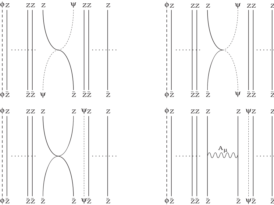
Figure 3: Feynman diagrams containing a single insertion of the interaction Hamiltonian. The two different impurities are labeled $\phi$ and $\psi$.

The first diagram arises from contractions where one $\phi$ field has “hopped” past a $Z$ field, in this case to the left. The exponential factor appearing in front of this term is $exp(2\pi in/J)$, since the amplitude for this term is

$$e^{2\pi ipn/J}\>e^{-2\pi i(p-1)n/J}\>\Big{\langle}\widetilde{{\cal O}}_{p}^{J}(x)\>\bar{\widetilde{{\cal O}}}_{p-1}^{J}(y)\Big{\rangle}$$ (VI.32)

There will also be a contribution from a diagram where a $\phi$ field hops to the right, and it will be associated with a factor $exp(-2\pi in/J)$, with the amplitude otherwise the same.

We will now compute the amplitude for this diagram at planar level, but only keep track of the divergent parts which determine the counterterm structure and eventually the anomalous dimension. In position space, this diagram consists of $J+2$ fields located at spacetime position $x$, interacting with $J+2$ fields located at $y$. The divergence arises from the loop at the center of the diagram, which corresponds to the integration over all spacetime (i.e. $\int d^{4}w$) of one insertion of the Hamiltonian and four propagators. The loop integral will contribute, beyond the tree level result,

$$\frac{1}{64\pi^{4}}\lambda e^{2\pi in/J}\int d^{D}w\frac{1}{|w-x|^{4}|w-y|^{4}}\sim\frac{1}{16\pi^{2}|x-y|^{4}}\frac{\lambda}{\epsilon}e^{2\pi in/J}$$ (VI.33)

where we have continued to $D=4-2\epsilon$ dimensions to regulate the ultraviolet divergence coming from $x\rightarrow w$ and $y\rightarrow w$, which now appears as a pole in $\epsilon$. We have the ’t Hooft coupling appearing here because a factor of $g^{2}_{YM}$ combines with a factor of $N$ at planar level when the first contraction across the traces are taken. We drop the contributions from the part of the diagram outside the interaction, since these do not modify the counterterm structure we are seeking. We see the appearance of the combination $\lambda/\epsilon$ appropriate to one-loop. We ignore the issue with infrared divergences when the external momenta vanish; these do not affect the anomalous dimension.

There are also diagrams in which $\phi$ and $Z$ fields interact, but which nonetheless do not lead to hopping. The hop-less diagrams in which $\phi$ and $Z$ fields interact arise in two ways. The first such diagram is similar to the one we considered above, but with a different ordering of the fields in the interaction term. There is also a diagram in which the interaction between the scalar $\phi$ and $Z$ fields is due to gluon exchange. These two diagrams contain the same divergences in their loops, but with opposite sign, and so their sum is finite. We ignore finite contributions since they do not give rise to anomalous dimensions.

The action (A.9) contains an interaction term in which only $Z$ fields interact with each other and a term in which $Z$ fields interact with gluons, and clearly lead to no hopping. Such interactions give rise to diagrams in which the four scalar $Z$ fields interact directly, and diagrams where their interaction is a result of gluon exchange. Both these diagrams contribute equal divergences with the same sign. The divergence part of these is the same as in (VI.33), but since there is no hopping, the exponential prefactor is missing. At planar level, there are $J-2$ possible ways the $Z$ fields can interact among each other.

The ultraviolet divergences in these diagrams can be removed by the addition of counterterms to the action to absorb the divergences. Computing the correlation function above, to one-loop, with an insertion of the composite operator, and including the counterterms appropriate to this order, we find the finite renormalized $Z_{{\cal O}}$, whose value is

$$Z_{{{\cal O}}_{n}}=1-\frac{\lambda}{8\pi^{2}\epsilon}\left(2e^{2\pi in/J}+2e^{-2\pi in/J}+(J-2)\right)$$ (VI.34)

where the first two terms absorb the divergences from the diagrams with one hop to the left or right respectively, with a factor of two multiplying the exponential due to the hopping, since we are considering composite operators with two impurities. The last term absorbs the divergences from the two diagrams which do not result in a hop and come from the interactions of $Z$ fields alone, and contribute $J-2$ such counterterms.

We are now almost ready to compute the anomalous dimension of the operator ${\cal O}_{n}$. The only remaining piece left to compute is the wave-function renormalizations of the individual fields which enter into the correlation function, as seen in (VI.28). There are three types of diagrams which modify the scalar propagators at one-loop. The wave-function renormalizations, which are the only kind of renormalization to the bare ${\cal N}=4$ propagators, are generated by diagrams in which a closed loop is constructed as in FIG. 4, and arise from gauge boson, fermion and scalar loops. Their computation is straightforward, and the resultant one-loop wave-function renormalization is

$$Z_{\phi}=Z_{Z}=1+\frac{1}{4\pi^{2}}\frac{\lambda}{\epsilon}$$ (VI.35)

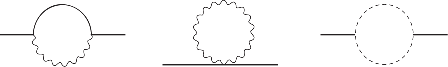
Figure 4: Diagrams contributing to the scalar wavefunction renormalization at one loop. The first is a scalar tadpole, the second a gauge boson loop, and the third a fermion loop.

The factor of $\lambda$ arise because there are two interaction vertices, each contributing $g_{YM}$, and a factor of $N$ enters due to the traces over color indices from the closed loop. Putting these together we have to first loop order

$$\mathcal{Z}_{n}=1-\frac{\lambda}{4\pi^{2}\epsilon}\left(e^{2\pi in/J}+e^{-2\pi in/J}-2\right)$$ (VI.36)

which yields the anomalous dimension

$$\gamma_{n}=-\>\frac{\lambda}{4\pi^{2}}\left(e^{2\pi in/J}+e^{-2\pi in/J}-2\right)$$ (VI.37)

We will meet this general from again in VI.4. The $2$ is a direct result of supersymmetry, since for $n=0$, the operator is BPS and hence protected against receiving quantum corrections. This is a manifestation of the BPS condition in the form (VI.22). Incidentally, we can decompose this result into the $c_{l,h}^{(n)}$ we met in (VI.30), whence $c_{1,1}^{(n)}=c_{1,-1}^{(n)}=1$ and $c_{1,0}^{(k)}=-2$.

We mention also that, had we separated the interaction Lagrangian into F and D-terms, at first loop we would have found that only the F-terms contribute, and the sum of all the diagrams with insertions of D-terms vanish, for two and three-point functions Constable et al. (2002); Kristjansen et al. (2002).

The anomalous dimension in (VI.37) has been computed for finite $J$. In the BMN limit, when $J$ is taken large, the anomalous dimension becomes

$$\gamma_{n}=n^{2}\>\lambda^{\prime}$$ (VI.38)

and we see explicitly the appearance of the new effective coupling $\lambda^{\prime}=\lambda/J^{2}$ because the ’t Hooft coupling $\lambda=g^{2}_{YM}N$ has combined with a $1/J^{2}$ from the expansion of the exponentials. We see that in the BMN limit the anomalous dimensions of BMN operators are finite, since $g^{2}_{YM}$ is held fixed while $N$ and $J$ are scaled such that $\lambda^{\prime}$ remains finite. Contrast this with a normal ’t Hooft expansion, in which the expansion parameter is $\lambda$, and this diverges in the BMN limit. This is a key result, since it tells us that in the double scaling limit, BMN operators will have finite, and hence well-defined, scaling dimensions, which can be compared to the string side of the duality. Recall that the exponentials entered as the diagonalizing matrix transforming the original basis of operators (VI.19) to one with well-defined scaling dimension, which we took to define one set of BMN operators. In turn, the precise structure of this matrix originated in the hopping behaviour embodied in the interaction Hamiltonian.

We can compare this result for anomalous dimensions of single-trace operators with two impurities to the string theory calculation of the mass spectrum for single-string states (IV.12), with excitations of the left and right moving oscillators at level $n$ in the plane-wave background. As we discussed in section V.2, the BMN correspondence states a relationship between the effective coupling in the gauge theory and in the BMN limit, and string theory parameters on the plane-wave background, which was stated in (I.11), (I.12) and (I.13). We noted earlier in section II.3.1 that $p^{+}$ is a central charge of the supersymmetry algebra of the plane-wave background, since its generator commutes with all the other generators of the algebra. As such, its value specifies a sector of the string theory, unmixed by actions of the isometry or string interactions. This is in distinct contrast to flat space, where the light-cone boosts can change $p^{+}$. Therefore it makes sense to think of $\alpha^{\prime}\mu p^{+}$ (or equally $\mu$ in a sector of fixed $p^{+}$) as an expansion parameter on the string side. The effective gauge theory expansion parameter $\lambda^{\prime}$ is related to the light-cone momentum, which is held fixed in the BMN double scaling limit, via (I.11). When the gauge theory is weakly coupled and $\lambda^{\prime}$ is small, the light-cone momentum $\alpha^{\prime}\mu p^{+}$ is large. This implies that the tension term in the light-cone string theory action (IV.7) dominates the gradient terms (since we’ve taken $\mu$ large), and the quantum mechanics of the string becomes that of a collection of massive particles. This has motivated the string bit model Vaman and Verlinde (2002); Verlinde (2002). Under these conditions, the mass spectrum (IV.12) can be expanded to first order, with the result that

$$\omega_{n}\approx\alpha^{\prime}\mu p^{+}\left(2+\frac{n^{2}}{(\alpha^{\prime}\mu p^{+})^{2}}\right).$$ (VI.39)

We use the relation ${\cal D}-{\cal J}=\Delta_{0}+\gamma-J$, which for the operator we have considered gives ${\cal D}-{\cal J}=2+\gamma$. We then have $\frac{2\omega_{n}}{\alpha^{\prime}\mu p^{+}}={\cal D}-{\cal J}$, after using (VI.38) and (I.11). The comparison is valid so long as $\lambda^{\prime}\ll 1/n^{2}$, or equivalently, when $|\alpha^{\prime}\mu p^{+}|\gg n$. For any finite $n$, we are free to choose $\lambda^{\prime}$ or $\alpha^{\prime}\mu p^{+}$ so that these conditions hold. This is our first direct test of the BMN conjecture, and it has passed with flying colors.

In this section, we computed anomalous dimensions of a class of BMN operators to first order in $g^{2}_{YM}$, and found that it reproduces the string theory calculation, giving a first test of the BMN conjecture. We may wonder whether this result extends to higher loops. The investigation of this question will be the focus of the next section, and we will show that the result indeed holds to all orders in perturbation theory.

VI.4 Anomalous dimension of the BMN operators, the planar result to all orders in $\lambda^{\prime}$

In this subsection we establish the anomalous dimensions of BMN operators in the BMN limit (I.7) and (I.8), to all orders in perturbation theory, and demonstrate its finiteness. We follow Santambrogio and Zanon (2002), relying heavily on superspace techniques and general results from conformal field theory. The two-point correlation function was first computed to order $g^{4}$, using $\mathcal{N}=1$ superspace techniques in Penati et al. (1999, 2001). This analysis was later extended by Santambrogio and Zanon (2002), in the planar limit (genus zero), perturbatively to all orders in the ’t Hooft coupling $\lambda^{\prime}$. The analysis relies heavily on restrictions on the form of quantum corrections to correlation functions in ${\cal N}=4$ super-Yang-Mills, arising from supersymmetry and conformal invariance.

The relevant ${\cal N}=4$ action, written in $\mathcal{N}=1$ language, together with the relevant superspace conventions, is presented in appendix A. The $U(1)_{J}$ subgroup we are interested in is the one which rotates one of the chiral superfields, which we choose to be $Z=\Phi^{3}$, corresponding to the real scalars in (V.3), and carrying one units of positive R-charge. The propagator for chiral superfields can be derived from (A.6) by expanding the exponentials in the first term, and then inverting the quadratic operator connecting $\Phi,\bar{\Phi}$, with the result

$$\begin{split}\langle\Phi_{ab}^{i}(z)\bar{\Phi}_{cd}^{j}(z^{\prime})\rangle=\frac{\delta^{ij}\delta_{ad}\delta_{bc}g_{YM}^{2}}{8\pi^{2}}\bar{D}^{2}D^{\prime 2}\frac{\delta^{4}(\theta-\theta^{\prime})}{|x-x^{\prime}|^{2}}\\ \langle\bar{\Phi}_{ad}^{i}(z)\Phi_{bc}^{j}(z^{\prime})\rangle=\frac{\delta^{ij}\delta_{ad}\delta_{bc}g_{YM}^{2}}{8\pi^{2}}D^{2}{\bar{D}^{\prime 2}}\frac{\delta^{4}(\theta-\theta^{\prime})}{|x-x^{\prime}|^{2}},\end{split}$$ (VI.40)

with the $U(N)$ adjoint indices explicitly indicated. The appearance (and the relative order) of the superspace differential operators in these propagators can be understood as follows. The fields appearing in the action (A.6) are to be interpreted as chiral superfields, and so the sum over these fields in the partition function must be constrained in an appropriate way. We may enforce such a constraint by introducing unconstrained potential superfields $\mathcal{U}$ (in a way analogous to Maxwell theory), and writing the chiral superfields as Weinberg (2000)

$$\Phi=\bar{D}^{2}\mathcal{U},$$ (VI.41)

whereby $\Phi$ is automatically chiral, satisfying $\bar{D}_{\dot{\alpha}}\Phi=0$. We then rewrite the action in terms of the potential superfields, with the partition function measure summing over all such field configurations, using (VI.41) in place of the chiral fields in the action. When computing correlation functions of chiral superfields, we use the new action with the insertions of chiral superfields replaced again according to (VI.41). A careful treatment then leads us to the form of the propagators in (VI.40) Weinberg (2000). In particular, the order of the two superderivatives in the two propagators will turn out to be important for our purposes, since they do not commute.

Now consider a general operator consisting of $h$ chiral fields and $\bar{h}$ anti-chiral fields. The propagators for these are given in (VI.40). We assume the free propagators are normal-ordered, and drop all singular terms arising from self contractions of such propagators (this is the limit $z\rightarrow z^{\prime}$). We’ll assume for simplicity that these fields are in the same $\mathcal{N}=1$ multiplet, and ignore the index $i$. We will suppress group indices below for notational clarity and denote such a composite operator as ${\cal W}_{h,\bar{h}}$. We are interested in computing the two-point correlator of ${\cal W}$ and its conjugate, $\langle{\cal W}_{h,\bar{h}}(z)\bar{{\cal W}}_{h,\bar{h}}(z^{\prime})\rangle$ in the free theory. As usual, this can be computed by taking Wick contractions to write the result as sums of products of the free propagators (VI.40). We do not trace over the group indices here, although for gauge invariant BMN operators such traces are in place. Taking traces changes some of the dependence on $N$ in the calculations below, but does not alter the anomalous dimension we arrive at in the end.

Some identities which will prove useful are listed in (A.5). The simplest case to consider, is of course, that of $h=1,\bar{h}=0$. We define the total dimension of the operator ${\cal W}_{h,\bar{h}}$ to be $\Delta=h+\bar{h}$, and the chiral weight to be $\omega=h-\bar{h}$. For this simple case, we have $\Delta=\omega=1$. This example gives rise to only a single propagator, and establishing the result amounts to applications of some simple superspace identities. We would like to rewrite the result in a form that makes clear the differences arising from the two propagators in the (VI.40), the source of which is the particular ordering of the chiral and anti-chiral derivatives. We also note that the term $\delta^{4}(\theta-\theta^{\prime})/|x-x^{\prime}|^{2}$ is symmetric in the primed and unprimed arguments, and so we are free to drop the prime on the derivatives. For both ordering of derivatives, $\bar{D}^{2}D^{2}$ and $D^{2}\bar{D}^{2}$, we use commutation relations to push one $D^{\alpha}$ to the left or one $D_{\alpha}$ to the right, such that both terms generate a factor of $D^{\alpha}\bar{D}^{2}D_{\alpha}/2$ plus a term proportional to $D^{\alpha}\bar{D}^{\dot{\alpha}}$, but with a relative sign difference depending on the original ordering. This sign difference will appear through the chiral weight, which counts the difference between numbers of the two types of propagators, and hence the two ordering of the superderivatives. For the simplest case we are considering, the result is simple and can be written as

$$\langle{\cal W}_{1,0}(z)\bar{{\cal W}}_{1,0}(z^{\prime})\rangle=C_{1,0}g_{YM}^{2}\left(\frac{1}{2}D^{\alpha}\bar{D}^{2}D_{\alpha}+\frac{i}{4}[D^{\alpha},\bar{D}^{\dot{\alpha}}]\sigma^{\mu}_{\alpha\dot{\alpha}}\partial_{\mu}\right)\frac{\delta^{4}(\theta-\theta^{\prime})}{|x-x^{\prime}|^{2}}\ .$$ (VI.42)

Care must be taken in deriving this expression to drop all singular terms which go like delta functions, arising from self contractions of the single propagator (i.e., dropping terms which vanish when $x\neq x^{\prime}$). They arise for example in the above case when $\Delta=1$ through $\Box|x-x^{\prime}|^{-2}$. These are removed by the normal-ordering prescription. The analysis of the case where $h=0,\bar{h}=1$, yields a similar result, with the difference that the commutator appears with opposite ordering. There is an overall normalization which we have absorbed into the constant $C_{1,0}$.

The next simplest case to consider is with $\Delta=\omega=2$, in which we simply include an additional chiral field. We need to evaluate the expression $\left(\bar{D}^{2}D^{2}(\delta^{4}(\theta-\theta^{\prime})|x-x^{\prime}|^{-2})\right)^{2}$, which is straightforward but tedious. We first expand the superderivatives using the Leibniz rule, then square the expression. This generates a large number of terms; however, many can be dropped by noting that they multiply together delta functions of Grassmann coordinates, or such delta functions and Grassmann coordinates; some of these terms will also involve products of superderivatives. Most of these terms then vanish because of the Grassmann nature of the delta functions and coordinates. Terms of the form $\delta^{4}(\theta-\theta^{\prime})F(D_{\alpha},\bar{D}_{\dot{\alpha}})\delta^{4}(\theta-\theta^{\prime})$ vanish unless all the $\theta$’s in the second delta function are removed by the combination of chiral and anti-chiral derivatives in $F$, and this implies that the only non-vanishing terms of this form are those for which $F$ contains at least two chiral and two anti-chiral derivatives; for the case with two pairs of such derivatives, the only terms which contribute are those without the partial derivative pieces in the superderivatives, since the partial derivatives are always paired with anticommuting coordinates. It also simplifies the calculation to always keep the remaining Grassmann delta function explicitly, without applying the Grassmann derivatives to it. Using the relation $\Box|x-x^{\prime}|^{-2\Delta}=4\Delta(\Delta-1)|x-x^{\prime}|^{-2(\Delta+1)}$ and the identities in (A.5), we can write the result as

$$\langle{\cal W}_{2,0}(z)\bar{{\cal W}}_{2,0}(z^{\prime})\rangle=C_{2,0}g_{YM}^{4}\left(D^{\alpha}\bar{D}^{2}D_{\alpha}+\frac{i}{2}[D^{\alpha},\bar{D}^{\dot{\alpha}}]\sigma^{\mu}_{\alpha\dot{\alpha}}\partial_{\mu}+\Box\right)\frac{\delta^{4}(\theta-\theta^{\prime})}{|x-x^{\prime}|^{4}}.$$ (VI.43)

Had we considered adding an anti-chiral field instead of a chiral field, so that $h=\bar{h}=1$, we would have found that both the commutator term (because we would have generated two commutators, but with opposite sign), and the Laplacian term would have vanished. The form of terms with successively more fields can be deduced in the same way, once the form of the previous one in the sequence is known, and this suggests an inductive derivation of the general result. Given the form for a correlator with an arbitrary number $h$ chiral and $\bar{h}$ anti-chiral fields, multiplying by another propagator for a chiral or anti-chiral field and performing superspace algebra as above, generates the form of the term with $h+1$ chiral or $\bar{h}+1$ anti-chiral fields.

If we assume that the result for $h$ chiral fields and no anti-chiral fields is proportional to

$$g_{YM}^{2h}\left(\frac{h}{2}D^{\alpha}\bar{D}^{2}D_{\alpha}+\frac{i}{4}[D^{\alpha},\bar{D}^{\dot{\alpha}}]\sigma^{\mu}_{\alpha\dot{\alpha}}\partial_{\mu}+\frac{h}{2}\Box\right)\left(\frac{\delta^{4}(\theta-\theta^{\prime})}{|x-x^{\prime}|^{2h}}\right),$$ (VI.44)

then we can find the result for $h+1$ chiral fields by noting

$$g_{YM}^{2(h+1)}\left(\frac{(h+a)}{2}D^{\alpha}\bar{D}^{2}D_{\alpha}+\frac{i(h+b)}{4}[D^{\alpha},\bar{D}^{\dot{\alpha}}]\sigma^{\mu}_{\alpha\dot{\alpha}}\partial_{\mu}+\frac{(h+c)}{2}\Box\right)\bar{D}^{2}D^{2}\left(\frac{\delta^{4}(\theta-\theta^{\prime})}{|x-x^{\prime}|^{2h}}\frac{\delta^{4}(\theta-\theta^{\prime})}{|x-x^{\prime}|^{2}}\right)=0,$$ (VI.45)

which vanishes because of the two delta functions. For $\bar{h}$ anti-chiral fields and no chiral fields, (VI.44) would be by replaced an equation in which $h\rightarrow\bar{h}$, and with the sign of the second term reversed. Judicious use of the Leibniz rule and dropping all terms which vanish because of the presence of too many Grassmann coordinates will generate a result of the form (VI.44) for which $a=b=c=1$. Had we reversed the order of $\bar{D}^{2}D^{2}$ (to $D^{2}\bar{D}^{2}$) in (VI.45), to add one more anti-chiral field, we would have arrived at $a=-b=c=1$. By induction, we arrive at the general form of the correlation function for arbitrary values of $h$ and $\bar{h}$ (still in the free theory),

$$\langle{\cal W}_{h,\bar{h}}(z)\bar{{\cal W}}_{h,\bar{h}}(z^{\prime})\rangle=C_{h,\bar{h}}g_{YM}^{2(h+\bar{h})}\left((h+\bar{h})D^{\alpha}\bar{D}^{2}D_{\alpha}+\frac{i(h-\bar{h})}{2}[D^{\alpha},\bar{D}^{\dot{\alpha}}]\sigma^{\mu}_{\alpha\dot{\alpha}}\partial_{\mu}+\frac{h(h-1)+\bar{h}(\bar{h}-1)}{2(h+\bar{h}-1)}\Box\right)\frac{\delta^{4}(\theta-\theta^{\prime})}{|x-x^{\prime}|^{h+\bar{h}}},$$ (VI.46)

for some overall constant $C_{h,\bar{h}}$ depending on the number of chiral and anti-chiral fields. In addition, the Laplacian term gives zero when $h=1,\bar{h}=0$ or $h=0,\bar{h}=1$.

We are now interested in computing the value of such correlation functions in the interacting theory, taking quantum corrections into account. We take advantage of the conformal invariance of the theory, which is preserved (by virtue of the ${\cal N}=4$ supersymmetry), in the quantum theory. As we have discussed in VI.2, conformal invariance fixes the form of the two and three point correlation functions. For two-point functions, the only modifications appear in corrected scaling dimensions, and the overall normalization of the correlation functions, which takes account of the allowed composite operator renormalizations. The scaling dimension of the operators differ from their classical dimensions through the introduction of anomalous dimensions, which vanish at zero coupling. The chiral weight is not renormalized because the chiral and anti-chiral fields receive the same anomalous dimensions, as CPT commutes with the scaling operator in the superalgebra. Therefore, the two-point function (VI.46) in the full interacting theory, written in terms of the scaling dimension $\Delta$ and chiral weight $\omega$, becomes

$$\langle{\cal W}_{h,\bar{h}}(z)\bar{{\cal W}}_{h,\bar{h}}(z^{\prime})\rangle=C_{h,\bar{h}}(g_{YM}^{2}N)g_{YM}^{2\Delta_{0}}\left(\Delta D^{\alpha}\bar{D}^{2}D_{\alpha}+\frac{i\omega}{2}[D^{\alpha},\bar{D}^{\dot{\alpha}}]\sigma^{\mu}_{\alpha\dot{\alpha}}\partial_{\mu}+\frac{\Delta^{2}+\omega^{2}-2\Delta}{2\Delta-1}\Box\right)\frac{\delta^{4}(\theta-\theta^{\prime})}{|x-x^{\prime}|^{2\Delta}},$$ (VI.47)

with the full scaling dimension $\Delta=\Delta_{0}+\gamma$ now the sum of the classical scaling and anomalous dimension. So far we have been considering a general $U(N)$ gauge theory at arbitrary $N$; however, we are interested in the BMN limit of such operators. The coefficients $C_{h,\bar{h}}$ are universal in the sense that they depend only on $h$ and $\bar{h}$, and not on the particular layout of the chiral and anti-chiral fields in the operator ${\cal W}_{h,\bar{h}}$.

At genus zero $C_{h,\bar{h}}(g_{YM}^{2},N)$ depends on $g_{YM}^{2}$ and $N$ through the ’t Hooft coupling $\lambda=g_{YM}^{2}N$. This is in fact where the assumption of planarity appears. Its dependence on the ’t Hooft coupling can be expanded in a power series, $C_{h,\bar{h}}(\lambda)\propto 1+\sum_{n=1}^{\infty}\lambda^{n}d^{n}_{h,\bar{h}}$, with an overall proportionality factor coming from the normalization of the propagators (VI.40).

We would now like to specialize our discussion, so far in the general ${\cal N}=4$ framework, to the case of BMN operators, such as those in (V.14). The ${\cal N}=4$ multiplet, when written in $\mathcal{N}=1$ language, consists of three chiral superfields. We single out one of these chiral superfields, which we take to be $Z=\Phi^{3}$. It carries unit charge under the $U(1)$ subgroup of the $SU(4)$ R-symmetry of the superalgebra, rotating the scalars $\phi^{5},\phi^{6}$ into each other. The total R-charge counts the number of $Z$ fields appearing in the correlation function. The remaining chiral superfields $\Phi^{1},\Phi^{2}$ are neutral under this $U(1)$.

For definiteness, we consider operators of the form

$$\begin{split}\mathcal{V}^{J}_{n}&=\sum_{p=0}^{J}e^{\frac{2\pi inp}{J}}Z^{p}\Phi^{1}Z^{J-p}\\ \mathcal{W}^{J}_{n}&=\sum_{p=0}^{J}e^{\frac{2\pi inp}{J}}Z^{p}\bar{\Phi}^{2}Z^{J-p},\end{split}$$ (VI.48)

which can be used as building blocks for operators having more impurities. As we discussed in section V, $n$ is the excitation level on the string side of the duality. The operators in (VI.48) are related to each other by supersymmetry (they sit in the same supermultiplet, up to charge conjugation), with the important consequence that they receive the same quantum corrections, and hence the same anomalous dimensions. The equations of motion governing the fields in (VI.48) can be used to relate the two set of operators in (VI.48). Interactions can be read off from the action (A.6), and connect the three chiral superfields via terms proportional to $\int d^{4}x\int d^{2}\theta{\rm Tr}\left(\Phi^{1}[\Phi^{2},Z]\right)+h.c.$, where the trace is taken with respect to the $U(N)$ indices. The equation of motion for $\Phi^{2}$ is derived after rewriting the chiral integrals as chiral derivatives,

$$D^{2}\Phi^{2}=-i\sqrt{2}\left(\bar{\Phi}^{1}\bar{Z}-\bar{Z}\bar{\Phi}^{1}\right),$$ (VI.49)

together with its conjugate. The trace in the interaction has disappeared; $\Phi^{2}$ on the left-hand side carries the same $U(N)$ matrix indices as the right-hand side, where $\Phi^{1}$ and $Z$ are multiplied in the matrix sense. (VI.49) allows us to relate $\mathcal{V}^{J}_{n}$ and $\mathcal{W}^{J}_{n}$. From the equations of motion we can show

$$\bar{D}^{2}\mathcal{W}^{J}_{n}=i\sqrt{2}\left(1-e^{\frac{-2\pi in}{J}}\right)\mathcal{V}^{J}_{n}\ .$$ (VI.50)

Using (VI.50) we can rewrite the two point function of two $\bar{D}^{2}\mathcal{W}^{J}_{n}$ as

$$\langle\bar{D}^{2}\mathcal{W}^{J}_{n}(z)D^{2}\mathcal{\bar{W}}^{J}_{n}(z^{\prime})\rangle=2\>\left(2-2\>cos(\frac{2\pi n}{J})\right)\langle\mathcal{V}^{J+1}_{n}(z)\mathcal{\bar{V}}^{J+1}_{n}(z^{\prime})\rangle.$$ (VI.51)

The correlation function on the right differs from that of $\mathcal{V}^{J}_{n}$ through the insertion of one $Z$. In the limit we are considering, any single impurity interacts with $Z$ fields within a finite number of places from the location of the impurity, implying that the renormalization of $\mathcal{V}^{J}_{n}$ and $\mathcal{V}^{J+1}_{n}$ at any order in the perturbative expansion are the same, and hence they receive the same anomalous dimension. Alternatively, we can argue that in the large $J$ limit these operators tend to each other, and hence receive the same corrections. Parenthetically, if we rewrite the prefactor in parentheses on the right-hand side above as $2-e^{i2\pi n/J}-e^{-i2\pi n/J}$, we see the similarity to (VI.37), with the $2$ being a consequence of supersymmetry, as we argued in VI.3.

We point out that these relations are derived using the equations of motion, and hence hold only on-shell. The important point to note is that it is the on-shell operators (built from fields satisfying the equations of motion) which appear in the correspondence; the duality relates these to on-shell string states, satisfying the Virassoro physical state constraints.

The number of chiral and anti-chiral fields appearing in $\mathcal{V}^{J}_{n}$ is $h=J+1,\bar{h}=0$, while for $\mathcal{W}^{J}_{n}$, $h=J,\bar{h}=1$, giving their classical scaling dimension and chiral weight as $\Delta=J+1,\ \omega=J=+1$ and $\Delta=J+1,\ \omega=J-1$ respectively. We now make use of the relation (VI.47) for the two-point function of composite operators assembled from chiral or anti-chiral superfields, using it to replace both sides of (VI.51). Using manipulations similar to those above to maneuver the $\bar{D}^{2}$ and $D^{2}$ into proper place, we then have, introducing $f(\lambda,\Delta,\omega)$, from which we have extracted the tree level normalization,

$$N_{0}^{J}f(\lambda,J+1,J-1)\left(\gamma^{2}+2\gamma\right)=4\>\left(1-cos(\frac{2\pi n}{J})\right)\>N_{0}^{J+1}f(\lambda,J+2,J+2),$$ (VI.52)

with $N_{0}$ defined in (V.9). Both sides are multiplying $\bar{D}^{2}D^{2}\delta^{4}(\theta-\theta^{\prime})/|x-x^{\prime}|^{2(J+2+\gamma)}$, which we have stripped. $f(\lambda,\Delta,\omega)$ tracks the overall quantum corrections to the operators, and may be expanded in a perturbative expansion in $\lambda$, for any $\Delta,\omega$, $f(\lambda,\Delta,\omega)=1+\sum_{n=1}^{\infty}\lambda^{n}f_{n}(\Delta,\omega)$. In the large $J$ limit, the factors of $f$ on both sides of (VI.52) tend to the same function (because their arguments approach each other), with subleading corrections in $J$ which we will drop. The factors of $N$ appearing in (VI.52) arise here because we are computing correlation functions of fields carrying matrix indices, and the fields in the composite operators $\mathcal{V}^{J}_{n}$ and $\mathcal{W}^{J}_{n}$ are multiplied in the matrix sense. The powers of $N$ appearing are those appropriate to the planar contractions. As a result, the anomalous dimension $\gamma$ is determined by solving a quadratic equation, with the solution

$$\gamma=-1+\sqrt{1-4\>N_{0}\>\left(cos(\frac{2\pi n}{J})-1\right)}\ .$$ (VI.53)

The other solution to the quadratic equation would yield a non-zero anomalous dimension in the free theory limit, and must be discarded. In the large $J$ limit, the anomalous dimension becomes

$$\gamma=-1+\sqrt{1+\lambda^{\prime}n^{2}}\ ,$$ (VI.54)

making evident the explicit dependence on the modified ’t Hooft coupling $\lambda^{\prime}$.

This result holds to all orders in perturbation theory, but only at the planar level, confirming the proposal of Berenstein et al. (2002b) for the mass spectrum of the corresponding string states, and thus provides a non-trivial check of the duality.

The above result can be generalized for BMN operator with more impurities, for example (V.23). The technique used to calculate the anomalous dimension remains the same, and revolves around the key equation (VI.50). Given any operator $\mathcal{V}^{J+1}_{n}$ with more impurities, we can find a corresponding operator $\mathcal{W}^{J+1}_{n}$ to which it can be related via an equation analogous to (VI.50) (which, however, is in general more complicated). The end result is a relation similar to (VI.52), which can then be solved for the anomalous dimension. The result is Gross et al. (2003); Gomis et al. (2003b)

$$\gamma_{n_{1}\dots n_{m}}=\sum_{i=1}^{m}\left(-1+\sqrt{1+n_{i}^{2}\lambda^{\prime}}\right)\ ,$$ (VI.55)

with the understanding that $\sum_{i}n_{i}\ll J$.

VI.5 Operator Product Expansions in the BMN subsector

In this section, we first present a brief review of the operator product expansion (OPE), then move on to discuss its relevance in the context of the BMN correspondence. The most salient point will be a demonstration of the closure of the BMN subsector of operators in the ${\cal N}=4$ super Yang-Mills theory, which can serve as a motivation for the selection of this class of operators. On the more practical side, the OPE will allow us to rewrite certain correlators involving multi-trace operators in terms of operator product expansions of single-trace operators in prescribed pinching limits. We will use this technique is section VII.4 to discuss three and higher point functions of BMN operators.

In quantum field theory, the product of operators is in general divergent if the location of any of the operators coincide, and require renormalization. For free fields, the divergence can be removed by normal-ordering the operator product, which amounts to subtracting the vacuum expectation value. However, in a general interacting theory, the product remains divergent even after normal-ordering. In the short distance (high momentum) limit, the operator product expansion (OPE) allows one to express the singular behaviour as

$$O_{i}(x)\>O_{j}(y)\>\sim\>\sum_{k}\>C_{ij}^{k}(x-y)\>O_{k}(y)\>+\>\text{non-singular terms}$$ (VI.56)

with the coefficients $C_{ij}^{k}(x-y)$ singular in the limit $x\rightarrow y$, and the other terms regular in this limit. The $O_{k}$ are assumed to form a linearly independent basis of local operators for the theory under consideration, which commute or anticommute among themselves. In a unitary conformal field theory, this basis can be taken to be orthonormal Di Francesco et al. (1997). The sum on the right-hand side of (VI.56) receives contributions from a finite number of terms in the limit $x\rightarrow y$. The OPE (VI.56) is to be understood as an operator relation, i.e., it holds as a matrix element between any sets of states, or equivalently, as an insertion into any expression of the form

$$\Big{\langle}\cdots O_{i}(x)\>O_{j}(y)\cdots\Big{\rangle}\>\sim\>\sum_{k}\>C_{ij}^{k}(x-y)\>\Big{\langle}\cdots O_{k}(y)\cdots\Big{\rangle},$$ (VI.57)

with $\cdots$ denoting other operators which lie a distance to $y$ is greater than $|x-y|$. In a general quantum field theory, the OPE is an asymptotic expansion and hence not convergent. In the special case of a conformal field theory, the OPE can be shown to converge, with radius of convergence given by the distance to the nearest operator other than those which coincide. The proof of the operator product expansion, under some restrictive assumptions, can be found in Zimmerman (1970). A general discussion of the operator product expansion in quantum field theory can be found in Weinberg (1996), while a discussion applicable to two-dimensional conformal field theory, for example string theory, can be found in Polchinski (1998a, b).

We have presented a discussion of two and three point functions in unitary conformal field theories in section VI.2. The arguments of that section can be applied also to the OPE coefficients, and a renormalization group equation for them can be derived. More importantly, the OPE of quasi-primary operators simplifies, after choosing an orthonormal basis of operators, into

$$\Big{\langle}\mathcal{O}_{i}(x_{1})\mathcal{O}_{j}(x_{2})\Big{\rangle}\>\sim\>\sum_{k}\frac{C_{ij}^{k}(g_{ym}^{2},N)}{|x_{12}|^{\Delta_{i}+\Delta_{j}-\Delta_{k}}}\mathcal{O}_{k}(x_{2}),$$ (VI.58)

where again, the form of quantum corrections is limited to anomalous dimensions and corrections to the OPE coefficients. For a single-trace BMN operator ${\cal O}_{k}^{J}$, the scaling dimension is $\Delta_{k}=J_{k}+\mathcal{I}_{k}+\gamma_{k}$, with $\mathcal{I}_{k}$ the engineering dimension of the impurities and $\gamma_{k}$ the anomalous dimension of the operator. We now wish to demonstrate the important result Chu et al. (2002b) that the operator product expansion of BMN operators is closed. Closure here is to be interpreted as follows: the OPE of BMN operators has an expansion where only BMN operators appear and the expansion coefficients are finite in the BMN limit. The OPE of a set of BMN operators with non-BMN operators has an expansion where the OPE coefficients vanish in the BMN limit. This is suggestive that in the double scaling limit, the operators of interest to us are in fact the BMN operators. This result is closely related to fact that the anomalous dimensions of non-BMN operators, which have some $\lambda$ dependence, which we take to $\infty$ in the double scaling limit, generically diverge in the BMN limit. In the operator product expansion (VI.58), we consider the case of two BMN operators on the left-hand side. The total $R$-charge of the two sides must match, as well as the total scaling dimensions (which is already included in (VI.58)). We separate the dependence on the scaling dimension of the operators as follows

$$\Big{\langle}\mathcal{O}_{i}(x_{1})\mathcal{O}_{j}(x_{2})\Big{\rangle}\>\sim\>\frac{1}{|x_{12}|^{\Delta_{i}+\Delta_{j}-J}}\sum_{k}C_{ij}^{k}(g_{ym}^{2},N)|x_{12}|^{\Delta_{k}-J}\mathcal{O}_{k}(x_{2})\ ,$$ (VI.59)

which is suggested by the R-charge. For BMN operators with a finite number of impurities, $\Delta_{i}+\Delta_{j}-J=\mathcal{I}_{i}+\mathcal{I}_{j}$ which is finite, where $\mathcal{I}_{i}$ is the dimension of the impurities in the BMN operator $\mathcal{O}_{i}$, and $J$ is taken to be the magnitude of the total R-charge $J=|J_{i}|+|J_{j}|$. Now, $\Delta_{k}-J=\mathcal{I}_{k}+\gamma_{k}$, using R-charge conservation, and it is positive by virtue of the BPS bound. This is either finite or infinite. Since $J$ is taken large, $\Delta_{k}-J$ finite implies $\mathcal{O}_{k}$ is a BMN operator. Otherwise $\Delta_{k}-J$ is infinite and $\mathcal{O}_{k}$ is non-BMN, but then $|x_{12}|^{\Delta_{k}-J}$ vanishes faster than $|x_{12}|^{J-\Delta_{i}-\Delta_{j}}$, and therefore the contributions of the non-BMN operators drop out of the OPE. This behaviour is a direct result of the finiteness of the anomalous dimensions of BMN operators, a feature of the double scaling limit we noted earlier, and the divergence of the anomalous dimensions of non-BMN operators in the same limit. This is another facet of the requirement that BMN operators have well-defined total scaling dimensions in the BMN limit. To summarize, only the set of BMN operators contribute to the sum in (VI.59).

One can also show, using the results of Lee et al. (1998); Mann and Polchinski (2003), that in the large $J$ limit, the OPE of a set of BMN operators with non-BMN operators has an expansion where the OPE coefficients vanish.

VII Strings on plane-waves from gauge theory II: interacting strings

Having carefully considered the planar structure of BMN operators, we are now ready to move on and examine non-planar corrections to quantities we have been studying in section VI, first considering higher genus corrections to two-point correlation functions of chiral-primary operators (these receive no loop, i.e. $\lambda^{\prime}$, corrections). The BMN limit of these correlators is examined, showing that in the double scaling limit, certain higher genus contributions survive. This result distinguishes the BMN limit from the standard ’t Hooft limit, wherein all contributions from higher genus diagrams are seen to vanish. This consideration will demonstrate explicitly the appearance of the genus counting parameter in the BMN limit. We next look at correlators of BMN (near-BPS) operators, first in the free field theory limit but with first non-planar contributions, and then after turning on interactions, computing the first non-trivial contributions in both the genus counting parameter and the modified ’t Hooft coupling $\lambda^{\prime}$. Mixing between single and multiple trace BMN operators, and the requisite re-diagonalization of the basis, leading the so called “improved BMN operators”, will play a central role in the precise formulation of the correspondence between gauge theory operators and string states. We collect the above results in an elegant form suggested by Gomis et al. (2002); Constable et al. (2002). Up to this point, our focus has been on the calculation of two-point functions of BMN operators; three and even higher point functions are introduced and some pathology in their behaviour noted.

VII.1 Non-planar contributions to correlators of chiral-primary operators

We review the expansion to all genus of the two-point functions of chiral-primary operators, which are protected against quantum corrections by virtue of being BPS. Hence, the results we present can be calculated in the free theory, but extend to all values of the coupling.

To gain some insight into the genus expansion, consider the simplest correlation function that receives contributions from higher genus diagrams, the two-point function of chiral-primary operators (V.9) with $J=3$ (the case of $J=2$ only receives planar corrections)

$$\Big{\langle}{\cal O}^{J}(x)\bar{{\cal O}}^{J}(0)\Big{\rangle}_{J=3}=\frac{1}{3N_{0}^{3}}\langle Z_{ab}Z_{bc}Z_{ca}\bar{Z}_{de}\bar{Z}_{ef}\bar{Z}_{fd}\rangle\ .$$ (VII.1)

There are six possible ways of applying Wick contractions. Three of these lead to a factor of $N^{3}$ from contractions (leaving aside for now the prefactor coming from the normalization). These correspond to the planar diagrams. Planar diagrams always generate the highest power of $N$, and hence are the ones that dominate a large $N$ expansion (for finite $J$). Planar diagrams are those which can be drawn on a sphere (a one-point compactification of the plane) without any lines crossing. There are also three (that this number equals $J$ is a coincidence) non-planar diagrams, of genus one. These are diagrams which can not be drawn on a sphere without crossing, but can be placed on a torus without crossing. They contribute a single power of $N$. One can see the structure more clearly by the following trick Kristjansen et al. (2002). Imagine that each trace corresponds to a loop on which we place beads corresponding to the individual fields $Z$ and $\bar{Z}$, white beads depicting $Z$’s and black ones for the conjugate fields $\bar{Z}$. The beads are free to move on the loop, but can’t be pushed past each other (their order is significant). Changing the ordering of two nearby beads corresponds to crossing or uncrossing the lines connecting them. For the case $J=3$, reversing the order of the beads on one of the loops while keeping the other loop’s ordering fixed exchanges planar and non-planar diagrams, showing how the ordering of the beads is relevant. The cyclicity of the trace is reflected in the fact that rotating the beads around the loop results in an identical loop. One of the possible non-planar contractions is depicted in FIG. 5 (the left figure).

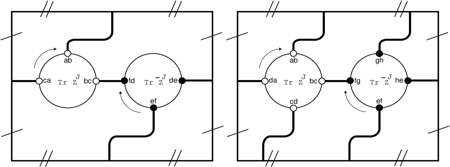
Figure 5: Irreducible toroidal diagrams contributing to $\langle{\rm Tr}Z^{J}{\rm Tr}\bar{Z}^{J}\rangle$. The arrows indicate the direction in which traces are taken.

For $J=3$, the maximum genus contributing is the torus. This trick can be generalized to higher $J$ and genus. First we need the notion of an irreducible diagram. Replace all lines in a diagram that are topologically parallel (call these reducible) with a single line (irreducible). The resulting diagram built only from irreducible lines is itself irreducible. Diagrams can be grouped into equivalence classes, where the equivalence is defined as follows: two diagrams are considered equivalent if they both collapse to the same irreducible diagram. For $J=4$ there are diagrams which reduce to the one we have already considered for $J=3$, and new ones which reduce to the one depicted in FIG. 5, the right figure. For higher $J$, all toroidal diagrams can be reduced to the two already considered. More generally, at genus $h$, the set of irreducible diagrams consists of those where the number of irreducible lines $l$ ranges between $l=2h+1$ and $l=4h$, which for genus one gives $l=3,4$ and for genus two the range is $l=5...8$ Kristjansen et al. (2002).

At genus one, for arbitrary $J\geq 3$, there are $J!/((J-3)!\>3!)$ ways of grouping the beads into three sets (the three irreducible lines in FIG. 5) while maintaining the order associated with the operator, and for for $J\geq 4$ the number of such groupings into sets of four is $J!/((J-4)!\>4!)$. We denote the number of inequivalent irreducible diagrams with $l$ irreducible lines at genus $h$ by $n_{h,l}$. The calculation of this number is the trickiest part of working out the combinatorics. For the cases we have already considered $n_{1,3}=1$ and $n_{1,4}=1$, while $n_{1,j}=0$ for $j>4$. However, for higher genus, there exist $n_{h,k}$ greater than one. The total number of diagrams in an equivalence class with $l$ irreducible lines for fixed $J$ can be found as follows: given a set of $J$ elements, place the elements into $l$ ordered distinct sets, maintaining the same overall cyclic ordering among all the elements. The number of possible ways of doing this is $J!/((J-l)!\>l!)$. The total number of diagrams at genus $h$ with $l$ irreducible lines for fixed $J$ is $n_{h,l}\>J!/((J-l)!\>l!)$. At fixed genus, to arrive at the total number of graphs we must sum up the contribution from graphs in all equivalence class for all allowed $l$. For the torus, this gives

$$n_{1,3}\left(\begin{matrix}J\\ 3\end{matrix}\right)\>+\>n_{1,4}\left(\begin{matrix}J\\ 4\end{matrix}\right)\>\approx\>\frac{J^{4}}{4!}\,,$$ (VII.2)

where in the last step we have shown the scaling in the large $J$ limit. Notice that sums of this form are always $N$ independent. The $N$ dependence in the combinatorics arise from traces over indices of Kronecker deltas appearing in the propagators (VI.1) and (VI.2) after all the Wick contractions are applied (of course keeping only diagrams at a fixed genus), and this dependence defines the genus order, via the standard ’t Hooft argument, where the suppression factor at any genus relative to the next lower genus goes like $1/N^{2}$ (or $1/N^{2h}$ relative to planar diagrams). As a result, in the BMN double scaling limit (I.8) (as opposed to the usual ’t Hooft limit), diagrams at all genera contribute to correlation functions, giving rise to a new effective expansion parameter $g_{2}^{2}=(J^{2}/N)^{2}$, which is fixed at an arbitrary but finite value and measures the relative contribution of each genus in perturbation theory. Contributions from diagrams at genus $h$ scale as $g_{2}^{2h}$. For the planar diagrams, there is an overall suppression by a factor of $J$ due to the normalization of the operators in (V.9), but a compensating enhancement by the same factor arising from the cyclicity of the trace (which amounts to the rotation of the beads on one of the loops relative to the other one). Putting together these observations, we arrive at the planar plus toroidal contribution to the two-point function of chiral-primary operators

$$\Big{\langle}{\cal O}^{J}(x)\bar{{\cal O}}^{J}(0)\Big{\rangle}=\frac{1}{|x|^{2J}}\left(1+\frac{g_{2}^{2}}{4!}+{\cal O}(g^{4}_{2})\right)\,.$$ (VII.3)

The normalization of the operator (V.9) is chosen to remove the overall dependence of the two-point function above on $N$ as well as the coupling $g^{2}_{YM}$ and factors of $8\pi^{2}$. Here we see the appearance of the parameter $g_{2}^{2}$ which organizes the expansion by genus. The planar diagrams contribute at order $g_{2}^{0}$ and the toroidal diagrams at order $g_{2}^{2}$. The new observation for the BMN double scaling limit is that the operators considered receive contributions from a number of diagrams which grow as $J^{4h}$ at genus $h$, but these are suppressed by $1/N^{2h}$, and the $J$ and $N$ dependence combine into the new effective expansion parameter $g_{2}^{2}$, appearing at genus $h$ as $g_{2}^{2h}$.

We will now describe a method for establishing the all orders (in $g_{2}^{2}$) result. We earlier mentioned two dimensional $QCD$ as a realization of ’t Hooft’s idea, and its exact solution via a matrix model Kostov and Staudacher (1997); Kostov et al. (1998). It turns out that many of the correlation functions we are interested in can be reduced to correlation functions in this matrix theory. Higher genus correlation functions in the complex matrix model, using loop equations, have been computed in Ambjorn et al. (1992). An alternative method for evaluating statistical ensembles of complex (or real) matrices can be found in Ginibre (1965); Mehta (1990). We will need only the most rudimentary results from matrix theory, which we collect here. Consider $N\times N$ complex matrices $Z_{ij}$, with $i,j$ running from $1$ to $N$, and define the measure $dZd\bar{Z}$ as

$$dZd\bar{Z}\>=\>\prod_{ij}\frac{1}{\pi}d(Re\>Z_{ij})d(Im\>Z_{ij})\,.$$ (VII.4)

The partition function over these matrices is defined as the above measure weighted by a Gaussian function

$$\mathcal{Z}\>=\>\int dZd\bar{Z}e^{-Tr(Z\bar{Z})}\,.$$ (VII.5)

The measure and the weight (and hence the partition function) are $U(N)\times U(N)$ invariant, representing independent multiplications on the left and the right. Correlation functions in this matrix model are defined as usual in QFT

$$\Big{\langle}\mathcal{O}(Z,\bar{Z})\Big{\rangle}_{MM}\>=\>\int dZd\bar{Z}e^{-Tr(Z\bar{Z})}\mathcal{O}(Z,\bar{Z})\,.$$ (VII.6)

The normalization of the measure is chosen so that $\langle 1\rangle=1$.

The correlation functions we study are not invariant under the full symmetry, but only under those generated by the diagonal subgroup, acting in the adjoint representation. For correlators built out of traces which do not mix $Z$ and $\bar{Z}$, the solution can be given by using character expansion techniques, expanding the correlation function in terms of group characters. These characters are orthogonal, with a proportionality constant that can be evaluated from group theory. The expansion coefficients are similarly computed from Young diagram considerations. We summarize the relevant result for two-point functions

$$\Big{\langle}{\rm Tr}Z^{J}{\rm Tr}\bar{Z}^{J}\Big{\rangle}_{MM}\>=\>\sum_{k=1}^{J}\prod_{i=1}^{k}(N-1+i)\prod_{m=1}^{J-k}(N-m)=\frac{1}{J+1}\left(\frac{\Gamma(N+J+1)}{\Gamma(N)}-\frac{\Gamma(N+1)}{\Gamma(N-J)}\right)\,,$$ (VII.7)

where have assumed $0<J<N$ in the last step. In the above, $N$ is the rank of the group $U(N)$ (we have kept $N$ finite thus far). Up to this point the results are exact.

Let us now return to the correlation function (VII.3). As we discussed in section VI.2 the spacetime dependence of this two-point function is completely fixed by the conformal invariance. Moreover, being chiral-primary the scaling dimension is also fixed by supersymmetry to the free field theory engineering dimension. These have already been made manifest in (VII.3). The remaining problem in computing (VII.3) is that of computing the dependence on factors of $J$ and $N$ arising from the combinatorics of all the Wick contractions. Separating out the spacetime dependence, and also the numerical and coupling constant factors in the scalar field propagators, the correlation function can be rewritten in terms of a correlation function in the matrix model we have described, which captures the combinatorics from evaluating all the traces over $U(N)$ color indices (producing both planar and non-planar contributions), as well as the combinatoric dependences on $J$,

$$\Big{\langle}{\rm Tr}(Z^{J}(x))\>{\rm Tr}(\bar{Z}^{J}(0))\Big{\rangle}=\left(\frac{g_{YM}^{2}}{8\pi^{2}|x|^{2}}\right)^{J}\Big{\langle}{\rm Tr}(Z^{J}){\rm Tr}(\bar{Z}^{J})\Big{\rangle}_{MM}\,,$$ (VII.8)

making use of the matrix model result (VII.7). We are interested in the large $J$ limit of (VII.8), and hence that of (VII.7). We can expand it as

$$\Big{\langle}{\rm Tr}Z^{J}{\rm Tr}\bar{Z}^{J}\Big{\rangle}_{MM}\>=\>J\>N^{J}\Bigg{[}1\>+\>\sum_{h=1}^{\infty}\>\sum_{k=2h+1}^{4h}\left(\begin{matrix}J\\ k\end{matrix}\right)\frac{n_{h,k}}{N^{2h}}\Bigg{]}\approx J\>N^{J}\Bigg{[}1\>+\>\sum_{h=1}^{\infty}\frac{n_{h,4h}}{(4h)!}\>\left(\frac{J^{4}}{N^{2}}\right)^{h}\>+\>\cdots\Bigg{]}\,,$$ (VII.9)

where in the last expression we have taken the large $J$ limit, and $\cdots$ denotes terms which vanish in the large $J$ and $N$ limit if we scale $J\sim\sqrt{N}$. We see that the genus counting parameter $g_{2}^{2}=J^{4}/N^{2}$ make a natural appearance in this limit. We will see in the next section when we come to consider non-BPS operators that this continues to be the case. In fact, this is another way to view the BMN limit: the limit is chosen precisely to ensure that the terms involving $n_{h,4h}$ in this limit remain finite and so we receive contributions from all genera. We can explicitly evaluate (VII.8) using (VII.9) in the BMN limit, giving for the chiral-primary operators

$$\Big{\langle}{\cal O}^{J}(x)\>\bar{{\cal O}}^{J}(0)\Big{\rangle}=\frac{1}{|x|^{2J}}\cdot\frac{\sinh\left(\frac{g_{2}}{2}\right)}{\frac{g_{2}}{2}}\,.$$ (VII.10)

Expanding this to first order in $g_{2}^{2}$ reproduces (VII.3).

VII.2 Non-planar contributions to BMN correlators

In this section we move onto the non-BPS (“almost-BPS”) BMN operators and compute the $g_{2}^{2}$ order non-planar contributions to their two-point functions, first at free field theory and then at first order in $\lambda^{\prime}$.

VII.2.1 Correlators of BMN operators in free gauge theory to first non-trivial order in $g_{2}$

Having studied the two-point function of chiral-primary operators to all orders, we are now ready to discuss the inclusion of phases in the more general BMN operators. We will concentrate on operators of the form (V.14) for $i\neq j$, and choose the notation $\phi_{i}=\phi$ and $\phi_{j}=\psi$. In this section we study the correlator in the free theory, postponing consideration of interactions to the next section. The correlator we are interested in is

$$\Big{\langle}{\cal O}^{J}_{ij,m}(x)\bar{{\cal O}}^{J}_{ij,n}(0)\Big{\rangle}_{0}\,.$$ (VII.11)

The calculation of the torus level contribution to the two-point function of BMN operators in the free gauge theory has been carried out along two different lines, using matrix model technology in Kristjansen et al. (2002), and via direct computation taking account of the combinatorics in Constable et al. (2002). We will see that the scaling with $N$ and $J$, in the BMN limit, is the same as for the chiral-primary operators, and $g_{2}^{2}=(J^{2}/N)^{2}$ will appear again as the genus counting parameter. We follow closely the presentation in Constable et al. (2002).

To count the number of Feynman diagrams that contribute to a two-point function at genus $h$, we draw a polygon with $4h$ sides, then place one operator at the center, and divide the other operator among the $4h$ vertices. We then pairwise identify all the sides and identify the vertices. All allowed diagrams are then generated by connecting the two operators via propagators, but without allowing the diagram to be collapsed to lower genus by shrinking homology cycles where no propagators have been placed. At genus $h$, the irreducible diagrams are those with $2h+1$ to $4h$ groups of lines. The number of ways of dividing $J$ lines into $4h$ sets is

$$\left(\begin{matrix}J\\ 4h\end{matrix}\right)=\frac{J!}{(J-4h)!(4h)!}\approx\frac{J^{4h}}{(4h)!}\,,$$ (VII.12)

where the last expression gives the behaviour at large $J$. A similar counting applies to the diagrams where we group the lines into $4h-1$ sets and so on, down to $2h+1$, but the number of such groupings is suppressed relative to the $4h$ case. For example, the case $4h-1$ yields

$$\left(\begin{matrix}J\\ 4h-1\end{matrix}\right)=\frac{4h}{J-4h+1}\left(\begin{matrix}J\\ 4h\end{matrix}\right)$$ (VII.13)

number of ways of distributing $J$ lines into $4h-1$ sets, and their contributions relative to the $4h$ groupings vanish in the BMN limit. This is the same behaviour we saw in the previous section at genus one, and it generalizes to arbitrary genus and for any finite number of impurities.

We can open up FIG. 5 for the torus diagrams with four groups of lines consisting of $J$ scalar fields $Z$ charged under $U(1)_{J}$ and two different scalar impurities we will label $\phi$ and $\psi$. Using the cyclicity of the trace, we can always place one of the impurities, say $\phi$, as the first field in each operator before applying contractions. This simplifies the counting since the position of the $\phi$ field is fixed, and we only have to worry about placing the $\psi$ field. The diagram can then be drawn as in FIG. 6.

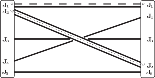
Figure 6: Diagram depicting the phase shift in a torus diagram with no interactions. The solid lines represent an arbitrary number of $Z$ fields and the dashed lines represent the contraction between two $\phi$’s or $\psi$’s.

Now there are five groups of fields, where the first one begins with the $\phi$ field. Let $J_{i}$ denote the number of fields, with $i=1,\ldots,5$ (with no $\psi$ field yet). We can place the $\psi$ field into any of these groups, and there are $J_{i}$ ways of doing so for the $i^{\rm th}$ group. Let us consider first the case where $m=n$ in (VII.11), so the two operators have similar phase structures. The two impurities may appear in the same group, in which case when we contract the fields in the two operators, the relative positions of $\phi$ and $\psi$ will remain fixed, and these diagrams will not contribute a phase factor. If the impurities are placed in different groups, then their relative positions in the two operators can in principle change, and the contractions will then be associated with a phase. For example, if $\psi$ is placed in the second group, then it will contract with a field in the conjugate operator where its relative position to the other conjugate scalar will have shifted by $J_{3}+J_{4}$ places, and this introduces a relative phase of $exp(2\pi in(J_{3}+J_{4})/J)$. Summing over all ways of placing $\psi$, we have for the two-point function the following expression

$$\Big{\langle}{\cal O}^{J}_{ij,m}(x)\bar{{\cal O}}^{J}_{ij,m}(0)\Big{\rangle}_{0}^{torus}=\frac{1}{JN^{J+2}}\left(\frac{1}{|x|^{2}}\right)^{J+2}N^{J}\sum_{J_{1}+\ldots+J_{5}=J+1}\ \ \sum_{k=1}^{5}J_{k}\ e^{2\pi im\theta_{k}/J}\,,$$ (VII.14)

with the phases defined as $\theta_{1}=\theta_{5}=0,\theta_{2}=J_{3}+J_{4},\theta_{3}=J_{4}-J_{2}$ and $\theta_{4}=J_{2}+J_{3}$. In performing the sum, we must impose the condition that $\sum_{i=1}^{5}J_{i}=J+1$. The first term on the right hand side is due to the normalization of the operators in (V.14). The next term arises from the propagators, with the normalization of the operators and propagators conspiring to remove the coupling and numerical factors. The last term comes from all the color index contractions at torus level. This expression is awkward, but can be turned into an integral representation in the large $J$ limit, with a delta function imposing the constraint, which can be evaluated explicitly. To see this, define $J_{i}=J\cdot j_{i}$. Then in the large $J$ limit, we can rewrite the two-point functions as

$$\Big{\langle}{\cal O}^{J}_{ij,m}(x)\bar{{\cal O}}^{J}_{ij,m}(0)\Big{\rangle}_{0}^{torus}=\left(\frac{1}{|x|^{2}}\right)^{J+2}\left(\frac{J^{2}}{N}\right)^{2}\prod_{k=1}^{5}\int_{0}^{1}\>dj_{k}\>j_{k}\>e^{2\pi im\theta_{k}/J}\delta(1-\sum_{l=1}^{5}j_{l})\,,$$ (VII.15)

and we again see the appearance of $J^{2}/N\equiv g_{2}$ which is held fixed in the BMN limit. The integral can be evaluated in a straightforward way. The construction when $m\neq n$ follows along the same lines, with the added complication that the position at which $\psi$ is inserted in each group becomes relevant, since the two operators have different phase structures. This more complicated situation has been considered in Constable et al. (2002); Kristjansen et al. (2002), and we present only the result. The final expression for the torus two-point function of BMN operators of the type we have been considering is

$$\Big{\langle}{\cal O}^{J}_{ij,m}(x)\,\bar{{\cal O}}^{J}_{ij,n}(0)\Big{\rangle}_{0}\>=\>\left(\frac{1}{|x|^{2}}\right)^{J+2}\left(\delta_{mn}\,+\,g_{2}^{2}\,M^{1}_{mn}\right)\,,$$ (VII.16)

for $i\neq j$ and where $g_{2}=J^{2}/N$, and with the matrix $M^{1}_{mn}$ is symmetric, i.e. $M^{1}_{mn}=M^{1}_{nm}$, and is defined as

$$M^{1}_{mn}=\begin{cases}0\ ,&m=0,n\neq 0\ \ \ \text{or}\ \ \ m\neq 0,n=0;\\ \frac{1}{24}\ ,&m=n=0;\\ \frac{1}{60}-\frac{1}{24\pi^{2}m^{2}}+\frac{7}{16\pi^{4}m^{4}}\ ,&m=n\neq 0;\\ \frac{1}{48\pi^{2}m^{2}}+\frac{35}{128\pi^{4}m^{4}}\ ,&m=-n\neq 0;\\ \frac{1}{4\pi^{4}(m-n)^{2}}\left(\frac{\pi^{2}}{3}+\frac{1}{m^{2}}+\frac{2}{n^{2}}-\frac{3}{2mn}-\frac{1}{2(m-n)^{2}}\right)\ ,&\text{all other cases.}\end{cases}$$ (VII.17)

The case of $m=0$ or $n=0$ corresponds to a two-point function with one of the composite operators being BPS; the $m=n=0$ gives the two-point function of BPS operators, while if $m\neq n$, but one of $m$ or $n$ zero, we see that the single-trace BPS operators do not mix with the non-BPS ones, at torus level. We expect the two-point function for $m=n=0$ to be exact to all orders in $g^{2}_{YM}$, since these operators are protected against receiving any anomalous dimensions. The non-BPS cases will receive $g^{2}_{YM}$ corrections, and we will discuss these corrections in section VII.2.2. The other cases show explicitly that in the free theory, single-trace non-BPS operators generically mix with each other, and this mixing begins at order $g_{2}^{2}$, where $g_{2}^{2}$ is the genus counting parameter. The discussion above can be generalized in an obvious way to higher genus diagrams in the free theory, with the genus $h$ contributions coming in at order $(g_{2}^{2})^{h}$.

VII.2.2 Correlators of BMN operators to first order in $\lambda^{\prime}$ and ${J^{2}}/{N}$

We have already computed the planar anomalous dimension to order $\lambda^{\prime}$ is section VI.3, and to all orders in section VI.4. We are now ready to move beyond planar level, but will work only to first order in $\lambda^{\prime}$. The duality would then put the result in correspondence with the string theory masses with loop corrections, giving a highly non-trivial test of the correspondence, and a step beyond what has been possible in the standard AdS/CFT correspondence.

The result will be proportional to $\lambda^{\prime}g_{2}^{2}$, showing that $g_{2}^{2}$ will continue to play the role of the genus counting parameter even with interactions switched on, and the role of the effective quantum loop counting parameter is still played by $\lambda^{\prime}$, in the BMN limit. The computation mirrors that of the previous section, but now taking account of the insertions of interaction terms. We only present an overview of the calculations; technical details can be found in Constable et al. (2002). At this order, only flavor changing interactions contribute, and therefore the only interactions of relevance are the so called F-terms which appear as the square of the commutator of scalars in different $\mathcal{N}=1$ chiral multiplets. We are considering two scalar impurity operators which are in $({\bf 1,9}$) of $SO(4)\times SO(4)$, they are symmetric in $i,j$ indices. Therefore the F-term which involves the commutator of the two impurities, being antisymmetric, does not contribute. The two impurities can therefore be considered separately, since they do not simultaneously enter into interactions, and only enter into interactions which are quadratic in the charged fields $Z$. These observations greatly reduce the number of possible diagrams which must be considered at this order.

There are three classes of Feynman diagrams to consider, involving nearest neighbor, semi-nearest neighbor and non-nearest neighbor. Nearest neighbor diagrams are the ones where two lines alongside each other are connected through an interaction term. One of these lines will always be an impurity. There are four possible interaction types coming from squaring the commutator in the interaction, all with equal weight, with those that switch the order of the impurity and charged field contributing a minus sign relative to those which do not. We must sum over all ways of building such diagrams by inserting a single interaction into the free diagrams, taking care with the phases from exchanges and the phase of the free diagram. The phase considerations parallel our discussion in the previous section. Summing all nearest neighbor diagrams, we find that the result (VII.16) of the previous section is simply modified by a logarithmic correction which merely changes the scaling dimension we computed at planar level, since the result does not involve $g_{2}$. The other two types of diagrams will, however, involve honest toroidal corrections.

The class of semi-nearest neighbor diagrams are those in which the fields entering an interaction are nearest neighbors in one of the composite operators, but not the other. These only contribute to the two-point function when $m\neq n$. For $m=n$ there are cancellations among semi-nearest neighbor diagrams. The number of such diagrams is suppressed relative to the nearest neighbor ones by $1/J$, but this is countered by an enhancement by a factor of $J$ because these diagrams have a different phase structure which in the large $J$ limit is larger by a factor $J$ relative to the nearest neighbor diagrams.

The non-nearest neighbor contributions do introduce logarithmic corrections whether or not $m\neq n$. These diagrams are rarer than the nearest neighbor one by a factor of $1/J^{2}$, but we again have an enhancement which compensates this, due to the phase structure. When we sum over all contributions from the above graphs, we must also consider the phase associated to the diagram from the placement of the second impurity, as we had to when considering the two-point function in the free theory.

The final result for the two-point function of the single-trace BMN operators we have been considering is

$$\Big{\langle}{\cal O}^{J}_{ij,m}(x)\,\bar{{\cal O}^{J}_{ij,n}}(0)\Big{\rangle}\>=\>\left(\frac{1}{|x|^{2}}\right)^{J+2}\Bigg{[}\delta_{mn}\left(1+\lambda^{\prime}L\,m^{2}\right)+\,g_{2}^{2}\,\left(M^{1}_{mn}\,+\,\lambda^{\prime}L\left(mnM^{1}_{mn}\,+\,\frac{\mathcal{D}^{1}_{mn}}{8\pi^{2}}\right)\right)\Bigg{]}\,,$$ (VII.18)

with $L=-\ln(|x|^{2}\Lambda^{2})$ and the matrix $M^{1}_{mn}$ given in (VII.17). This result holds for $i\neq j$. The matrix $\mathcal{D}^{1}_{mn}$ is

$$D^{1}_{mn}=\begin{cases}0\ ,&m=0\ \ \ \text{or}\ \ \ n=0;\\ \frac{2}{3}+\frac{5}{\pi^{2}n^{2}}\ ,&m=n\neq 0\ \ \ \text{or}\ \ \ m=-n\neq 0;\\ \frac{2}{3}+\frac{2}{\pi^{2}m^{2}}+\frac{2}{\pi^{2}n^{2}}\ ,&\text{all other cases.}\end{cases}$$ (VII.19)

The next question of interest, the significance of which would become clear in the next subsection, is the correlation function of a single-trace operator and a double-trace one, and two-point functions of double-trace operators. The double-trace operators have been defined in (V.11), (V.13) and (V.21). The double-trace operators (V.21) contain two scalar impurities, and as discussed in section V.3.3 can be in $({\bf 1},{\bf 9})$, $({\bf 1},{\bf 3^{\pm}})$ or $({\bf 1},{\bf 1})$ tensor representations of $SO(4)\times SO(4)$. BPS operators do not occur in the antisymmetric representation of ${\cal T}^{J,r}_{ij,n}$, since ${\cal O}^{J}_{[ij],n}=-{\cal O}^{J}_{[ij],-n}$. The correlators of non-singlets have been computed Beisert et al. (2003b), with the result

$$\begin{split}\Big{\langle}{\cal T}^{J,r}_{ij}(x)\,\bar{{\cal T}}^{J,s}_{ij}(0)\Big{\rangle}&=\left(\frac{1}{|x|^{2}}\right)^{J+2}\,\delta_{rs}\,,\\ \Big{\langle}{\cal T}^{J,r}_{ij,m}(x)\,\bar{{\cal T}}^{J,s}_{ij,n}(0)\Big{\rangle}&=\left(\frac{1}{|x|^{2}}\right)^{J+2}\,\delta_{rs}\delta_{mn}\left(1+\lambda^{\prime}L\,\frac{m^{2}}{r^{2}}\right)\,,\\ \Big{\langle}{\cal T}^{J,r}_{ij,m}(x)\,\bar{{\cal T}}^{J,s}_{ij}(0)\Big{\rangle}&=0\,,\end{split}$$ (VII.20)

$(i\neq j)$, up to order $\lambda^{\prime}$ and $g_{2}$. We see that the double-trace operators are diagonal to order $g_{2}$. Their mixing, like the single trace operators, begins at order $g_{2}^{2}$. We are considering here the $SO(4)$ non-singlet operators, but not making a distinction between the 9 and ${\bf 3^{\pm}}$ representations. The results for the singlet representations are complicated by the inclusion of the ${\rm Tr}(Z^{\dagger}Z^{J+1})$ term in the definition (V.14). The 9, ${\bf 3^{\pm}}$ and 1 representations all receive the same anomalous dimensions, and this degeneracy is a result of supersymmetry (cf. discussions of section V.3.3). Starting from any one of these representations we may reach the others by transformations generated by combinations of supercharges, and these combinations commute with the dilatation operator.

The single and double-trace operators mix at order $g_{2}$, with the overlaps, at first order in $\lambda^{\prime}$ being

$$\begin{split}\Big{\langle}{\cal T}^{J,r}_{ij,m}(x)\,\bar{{\cal O}}^{J}_{ij,n}(0)\Big{\rangle}&=\left(\frac{1}{|x|^{2}}\right)^{J+2}\frac{g_{2}}{\sqrt{J}}\frac{r^{3/2}\sqrt{1-r}\sin^{2}(\pi nr)}{\pi^{2}(m-nr)^{2}}\left(1+\frac{\lambda^{\prime}L\,(m^{2}-mnr+n^{2}r^{2})}{r^{2}}\right)\,,\\ \Big{\langle}{\cal T}^{J,r}_{ij}(x)\,\bar{{\cal O}}^{J}_{ij,n}(0)\Big{\rangle}&=\left(\frac{1}{|x|^{2}}\right)^{J+2}\frac{g_{2}}{\sqrt{J}}\left(\delta_{n,0}r-\frac{\sin^{2}(\pi nr)}{\pi^{2}\,n^{2}}\right)\left(1+\lambda^{\prime}Ln^{2}\right)\,.\end{split}$$ (VII.21)

Don’t be alarmed by the appearance of $1/\sqrt{J}$ in these expressions. When we come to rediagonalize the single-trace operators in the next section, we will see that the $1/J$ terms are compensated by sums (over $r$), and the two-point functions of the rediagonalized single-trace operators will receive contributions from such terms.

Extracting an overall power of $g_{2}$ in expression like (VII.21), the remaining terms can be arranged into an expansion in powers of $g_{2}^{2}$, i.e. in terms of planar and non-planar diagrams.

At this order in $g_{2}$, there are non-zero overlaps between double and triple trace operators, and at order $g_{2}^{2}$ even overlaps between single-trace and triple-trace operators. More generally, the overlap of a single-trace operator with any $t$-trace operator begins at order $g_{2}^{t-1}$. We have ignored these corrections since they do not affect the anomalous dimensions of single-trace operators at order $g_{2}^{2}$.

VII.3 Operator mixings and improved BMN conjecture

The results of the previous two sections have been computed and presented in the BMN basis. These results are to be compared to those on the string theory side of the duality according to the identification (V.8), in which we are instructed to compare the eigenvalue spectrum of the string field theory Hamiltonian to the spectrum of the dilatation operator minus the R-charge in gauge theory. This is a basis independent comparison. Alternatively, we may compare the matrix elements of the operators on the two sides of the duality. On the other hand, the two sides of the duality involve different Hilbert spaces, and the mapping between the bases of these distinct Hilbert spaces is part of the statement of the duality. Denote the basis on the gauge theory side by $\{|\,\mathfrak{a}\,\rangle{}_{{}_{gauge}}\}$ and on the string theory side by $\{|\,\tilde{\mathfrak{a}}\,\rangle{}_{{}_{string}}\}$, with $\mathfrak{a}$ labeling gauge theory states, and $\tilde{\mathfrak{a}}$ the labels on the string side. We need an isomorphism between the states of the two theories

$$\{|\,\mathfrak{a}\,\rangle{}_{{}_{gauge}}\}\leftrightarrow\{|\,\tilde{\mathfrak{a}}\,\rangle{}_{{}_{string}}\}\,,$$ (VII.22)

under the condition that the inner products on both sides agree

$${}_{{}_{gauge}}\langle\,\mathfrak{a}\,|\,\mathfrak{b}\,\rangle{}_{{}_{gauge}}\>=\>{}_{{}_{string}}\langle\,\tilde{\mathfrak{a}}\,|\,\tilde{\mathfrak{b}}\,\rangle{}_{{}_{string}}\,.$$ (VII.23)

The duality, in the proper basis, holds between these matrix elements

$${}_{{}_{gauge}}\langle\,\mathfrak{a}\,|\,\left(\mathcal{D}-\mathcal{J}\right)\,|\,\mathfrak{b}\,\rangle{}_{{}_{gauge}}\>=\>{}_{{}_{string}}\langle\,\tilde{\mathfrak{a}}\,|\,\frac{H}{\mu}\,|\,\tilde{\mathfrak{b}}\,\rangle{}_{{}_{string}}\,.$$ (VII.24)

In section V.3.3 the text around (V.19) (the second part of the SYM/plane-wave duality), we introduced a specific mapping between the Hilbert spaces on the either sides of the duality, however, we warned the reader that (VII.23) does not hold for the identification (V.19) (more precisely it only holds at $g_{2}^{0}$ level). In this section we intend to refine the dictionary between the gauge theory and string theory Hilbert spaces taking account of higher $g_{2}$ orders.

On the string theory side, there is a natural basis, the one which diagonalizes the free string theory Hamiltonian. We will refer to this basis as the free-string basis. In this basis, $m$-string states are orthogonal to $n$-string states for $m\neq n$, and in fact this basis is orthonormal (cf. discussions of section IV.3). The interactions induce mixings between these states; this basis does not diagonalize the full string field theory Hamiltonian. For example, at order $g_{s}$, the cubic string field theory Hamiltonian will cause transitions between one and two string states.

On the gauge theory side we start with the BMN basis, but if we are interested in the full scaling dimensions, including the anomalous dimensions, then we should choose a basis which diagonalizes the dilatation operator. This basis is referred to as the $\Delta$-BMN basis Georgiou et al. (2003). Incidentally, in this basis the operators are conformal primaries, and this is the basis in which the two and three-point functions take the forms (VI.16) and (VI.16) required by conformal invariance. This basis would correspond to the one on the string theory side that diagonalizes the full string field theory Hamiltonian, and is not the free-string basis we defined above. The basis of BMN operators we have been working with above are neither of these. They have well-defined scaling dimensions at planar level, but non-planar corrections induce non-diagonal mixings between the single-trace operators and between single and multi-trace operators in general. For example, at toroidal level, the classical ($\lambda^{\prime}=0$) scaling dimensions are no longer well-defined because of order $g_{2}^{2}$ mixings. This is seen easily by noting that single and double-trace BMN operators overlap at order $g_{2}$ (VII.21), and shows up at order $g_{2}^{2}$ in two-point functions of single-trace operators (VII.18).

The results of section VII.2.1 can be cast in the form

$$|x|^{2\Delta_{0}}\>\Big{\langle}{\cal O}_{\mathfrak{a}}(x)\bar{{\cal O}}_{\mathfrak{b}}(0)\Big{\rangle}=G_{\mathfrak{a}\mathfrak{b}}-\lambda^{\prime}\Gamma_{\mathfrak{a}\mathfrak{b}}\ln(|x|^{2}\Lambda^{2})\>+\>{\cal O}(\lambda^{\prime 2})\,,$$ (VII.25)

written in the BMN basis. We have introduced a notation whereby the indices $\mathfrak{a}$ range over single, double and in general $n$-trace operators, and the operators within each such class. This expression is written up to first order in $\lambda^{\prime}$, with the remaining terms of higher order in $\lambda^{\prime}$. $\Delta_{0}$ is the classical (non-anomalous) scaling dimension. The matrix $G_{\mathfrak{a}\mathfrak{b}}$ is the inner product on the Hilbert space of states created by the BMN operators, and $\Gamma_{\mathfrak{a}\mathfrak{b}}$ is the matrix of anomalous dimensions.

The free-string basis can be constructed on the gauge theory side by taking linear combinations of the original BMN operators

$$|\,\mathfrak{a}\,\rangle{}_{{}_{gauge}}\>=\>\mathcal{U}_{\mathfrak{a}\mathfrak{b}}{\cal O}_{\mathfrak{b}}(0)|\,0\,\rangle{}_{{}_{gauge}}\,,$$ (VII.26)

with the BMN operator ${\cal O}_{\mathfrak{a}}$ acting on the gauge theory vacuum. When $g_{2}$ vanishes, this basis coincides with the original BMN basis. Therefore, at order $g_{2}^{0}$ the change of basis matrix $\mathcal{U}$ is simply the identity.

Perturbative corrections in powers of $g_{2}$ results in a mixing between BMN operators with different numbers of traces, and we must rediagonalize this set of operators at each order in $g_{2}$ to maintain orthonormality of the inner product $G_{\mathfrak{a}\mathfrak{b}}$, to preserve the isomorphism with the free-string basis. The change of basis is chosen such that

$$\mathcal{U}G\mathcal{U}^{\dagger}=1\,,$$ (VII.27)

leading to

$${}_{{}_{gauge}}\langle\,\mathfrak{a}\,|\,\left(\mathcal{D}-\mathcal{J}\right)\,|\,\mathfrak{b}\,\rangle{}_{{}_{gauge}}\>=\>\left(\mathcal{U}(\Delta_{0}-J)G\mathcal{U}^{\dagger}+\mathcal{U}\Gamma\mathcal{U}^{\dagger}\right)_{\mathfrak{a}\mathfrak{b}}\>=\>n\delta_{\mathfrak{a}\mathfrak{b}}+\tilde{\Gamma}_{\mathfrak{a}\mathfrak{b}}\,,$$ (VII.28)

with $n$ counting the number of impurities in the operator ${\cal O}_{\mathfrak{a}}(0)$ creating the state $|\,\mathfrak{a}\,\rangle{}_{{}_{gauge}}$, and $\tilde{\Gamma}$ the anomalous dimension matrix in the free-string basis. In the basis where the inner product $G$ is diagonal, the anomalous dimension matrix is symmetric. The matrix elements (VII.28) are to be compared to the matrix elements of the string field theory Hamiltonian in the free-string basis. We will return to this in section VIII.

The change of basis implemented by $\mathcal{U}$ is not unique, but all such choices are related by orthogonal transformations. We may make a unique choice, with one subtlety involving BPS operators which we mention momentarily, by requiring that the matrix $\mathcal{U}$ implementing the change of basis (VII.27) be a real symmetric matrix. This turns out to be the choice for which the matrix elements of the rediagonalized operators can be matched to the matrix elements on the string side in the free-string basis. As we have already pointed out, in the BMN basis, single-trace BPS operators do not mix with single trace non-BPS operators, and likewise for pairs of double-trace operators, but they may mix with each other. However, this mixing does not involve $\lambda^{\prime}$ corrections since both operators are BPS. This mixing will not affect the anomalous dimensions. A similar pattern occurs in the string field theory, where the sums over intermediate BPS states do not alter the string masses. The dictionary translating between the string and gauge theory sides of the duality then seems to contain ambiguities for the BPS operators and their corresponding string states Beisert et al. (2003b); for example, we are unable to distinguish between single string and double string vacuum states, as well as single and double graviton states. We will comment on this point briefly in section IX. However, mixing between BPS and non-BPS operators can be dealt with by choosing a basis in which BPS operators do not mix with non-BPS operators, regardless of the number of traces; however, the degeneracy in the BPS subspace remains.

We expand the diagonalizing matrix, the inner product matrix and the matrix of anomalous dimensions, to order $g_{2}$:

$$\mathcal{U} =1 +g_{2}\mathcal{U}^{(1)} +{\cal O}(g_{2}^{3})\,,$$

$$G =1 +g_{2}G^{(1)} +\mathcal{O}(g_{2}^{3})\,,$$ (VII.29)

$$\Gamma =\Gamma^{(0)} +g_{2}\Gamma^{(1)} +{\cal O}(g_{2}^{3})\,.$$

$\mathcal{U}$ and $G$ are the identity at zeroth order in $g_{2}$ since the BMN operators start mixing among each other only at order $g_{2}$ for single-trace and double-trace overlaps, and at order $g_{2}^{2}$ for single-trace overlaps with single-trace with double-trace intermediate channels, while the non-vanishing of $\Gamma^{(0)}$ to this order captures the first order (in $\lambda^{\prime}$) anomalous dimensions of the unmixed BMN operators.

Inserting the expansions (VII.3) in (VII.27), we find that the change of basis matrix $\mathcal{U}$, to order $g_{2}$ involves the term of the same order in the expansion of the inner product matrix, and since $\mathcal{U}$ is unitary, we have

$$\mathcal{U}^{(1)}\>=\>-\frac{1}{2}G^{(1)}\,.$$ (VII.30)

We may also solve for $\tilde{\Gamma}$ to first order in $g_{2}$, using (VII.28) and expanding $\tilde{\Gamma}$ as above in (VII.3), with $\tilde{\Gamma}^{(0)}=\Gamma^{(0)}$. This yields

$$\tilde{\Gamma}^{(1)}=\Gamma^{(1)}-\frac{1}{2}\{G^{(1)},\Gamma^{(0)}\},$$ (VII.31)

We then have for the order $g_{2}$ rediagonalized matrix of anomalous dimensions

$$\tilde{\Gamma}^{(1)}=\left(\begin{matrix}0&\tilde{\Gamma}^{(1)}_{n,qs}&\tilde{\Gamma}^{(1)}_{n,s}\\ \tilde{\Gamma}^{(1)}_{pr,m}&0&0\\ \tilde{\Gamma}^{(1)}_{r,m}&0&0\end{matrix}\right)\,,$$ (VII.32)

In writing this matrix, we have chosen to discard the entries corresponding to the BPS operators ${\cal O}_{ij,n=0}^{J}$ and the combination $\sqrt{r}{\cal T}^{J,r}_{ij,n=0}+\sqrt{1-r}{\cal T}^{J,r}_{ij}$. This combination is chosen because it is orthogonal to ${\cal O}_{ij,n}^{J}$, $n\neq 0$, which can be easily seen from (VII.21). The sub-matrix involving these BPS operators can be diagonalized using the freedom we mentioned in the discussion following (VII.28). The remaining basis elements are chosen to correspond to the non-BPS single and double trace BMN operators given in ${\cal O}_{ij,n}^{J},\ {\cal T}^{J,r}_{ij,n}$ ($n\neq 0$) and $\sqrt{1-r}{\cal T}^{J,r}_{ij,n=0}-\sqrt{r}{\cal T}^{J,r}_{ij}$, in order. The entries of (VII.32) in this basis can be read off from (VII.21), and are

$$\tilde{\Gamma}^{(1)}_{n,r} =\tilde{\Gamma}^{(1)}_{r,n}=-\frac{\sin^{2}(\pi nr)}{\sqrt{J}2\pi^{2}}\,$$ (VII.33a)

$$\tilde{\Gamma}^{(1)}_{n,pr} =\tilde{\Gamma}^{(1)}_{pr,n}=\frac{\sqrt{1-r}}{\sqrt{Jr}}\frac{\sin^{2}(\pi nr)}{2\pi^{2}}\,.$$ (VII.33b)

This procedure can be continued to higher orders in $g_{2}$ in an obvious way.

To read off the anomalous dimensions, we must choose a basis which diagonalizes the dilatation operator. This basis would simultaneously diagonalize both the matrices $G_{\mathfrak{a}\mathfrak{b}}$ and $\Gamma_{\mathfrak{a}\mathfrak{b}}$. That such a diagonalization is possible (i.e. that these two matrices commute), can be argued from conformal invariance, since it implies that a basis of operators with definite scaling dimensions (classical plus anomalous) can be chosen. This choice of basis has been presented in Constable et al. (2002); Beisert et al. (2003b). Going to the $\Delta$-BMN basis, we find for the scaling dimension of single-trace BMN operators with two impurities, at order $g_{2}^{2}$,

$$\Delta=\Delta_{0}+\lambda^{\prime}\left(n^{2}+g_{2}^{2}\left(\frac{1}{48\pi^{2}}+\frac{35}{128\pi^{4}n^{2}}\right)\right)\,,$$ (VII.34)

for $n\neq 0$ and with $\Delta_{0}=J+2$ for two impurities. For $n=0$, the classical scaling dimension is protected against quantum corrections by virtue of supersymmetry. (VII.34) is the main (basis independent) result of this section, to be directly compared with the corresponding string field theory results of section VIII.

VII.4 $n$-point functions of BMN operators

Up to this point we have dealt with two-point functions of BMN operators, taking into account both non-planar corrections and interactions. We may wonder what role higher $n$-point functions play in the plane-wave/SYM duality. We address this issue in the context of three and four-point functions below.

VII.4.1 Three point functions of BMN operators

As discussed in section VI.2, the spacetime dependence of three-point functions in a conformal field theory is completely fixed and once a basis of quasi-primary operators is chosen, two and three point functions take the form of (VI.16) and (VI.17). Moreover, in such basis the operator product expansion takes a particularly simple form of (VI.58). The remaining task is then to find $C_{\Delta_{i},\Delta_{j},\Delta_{k}}(g_{YM}^{2},N)$. Taking the pinching limit of the three-point function (VI.17) (e.g. $x_{1}\rightarrow x_{2}$) and using the operator product expansion together with the the special form for two-point functions of quasi-primary operators, we can compute $C_{\Delta_{i},\Delta_{j},\Delta_{k}}(g_{YM}^{2},N,J)$ as a sum over $C_{ij}^{k}(g_{YM}^{2},N,J)$, where the sum runs over the non-singular constant terms in the OPE and with the dimension of the OPE coefficient equal to that of the third operator away from the pinching. We see that three-point functions of BMN operators carry no extra information beyond those of two-point functions. As an aside, one may use the fact that three-point functions have a simple form in a basis of quasi-primary operators (VI.17) as a check of gauge theory computations.

Here, however, we present the three-point function of chiral-primary operators. These correlators are protected against quantum corrections Lee et al. (1998); D’Hoker et al. (1999b, a). Furthermore, for chiral-primary operators the anomalous dimension vanishes, therefore

$$\Big{\langle}{\cal O}^{J_{1}}(x){\cal O}^{J_{2}}(y)\bar{{\cal O}}^{J_{3}}(0)\Big{\rangle}\>=\>\frac{1}{|x|^{2J_{1}}|y|^{2J_{2}}}\Big{\langle}{\rm Tr}Z^{J_{1}}{\rm Tr}Z^{J_{2}}{\rm Tr}\bar{Z}^{J_{1}+J_{2}}\Big{\rangle}_{MM},$$ (VII.35)

where $J_{1}+J_{2}=J_{3}$, and vanishing otherwise. The correlator on the right-hand side is a correlator in the Matrix model introduced in section VII.1 and using the Matrix theory techniques we can evaluate them to all orders in the genus expansion Kristjansen et al. (2002)

$$\begin{split}\Big{\langle}{\rm Tr}Z^{J_{1}}{\rm Tr}Z^{J_{2}}&{\rm Tr}\bar{Z}^{J_{1}+J_{2}}\Big{\rangle}_{MM}=\left(\sum_{k=J_{2}+1}^{J_{1}+J_{2}}-\sum_{k=1}^{J_{1}}\right)\prod_{i=1}^{k}(N-1+i)\prod_{m=1}^{J_{1}+J_{2}-k}(N-m)\\ &=\frac{1}{J_{1}+J_{2}+1}\biggl{(}\frac{\Gamma(N+1)}{\Gamma(N-J_{1}-J_{2})}+\frac{\Gamma(N+J_{1}+J_{2}+1)}{\Gamma(N)}-\frac{\Gamma(N+J_{1}+1)}{\Gamma(N-J_{1})}-\frac{\Gamma(N+J_{1}+1)}{\Gamma(N-J_{1})}\biggr{)}\\ &\simeq\sqrt{\frac{J_{1}+J_{2}}{J_{1}J_{2}}}\frac{\sinh\left(\frac{J_{1}(J_{1}+J_{2})}{2N}\right)\sinh\left(\frac{J_{2}(J_{1}+J_{2})}{2N}\right)}{\frac{\left(J_{1}+J_{2}\right)^{2}}{2N}}\,,\end{split}$$ (VII.36)

where the first equality is obtained assuming (without loss of generality) that $0<J_{1},J_{2}<N$ and in the final step we have taken the BMN limit $J_{1},J_{2}\sim\sqrt{N}\to\infty$ and $J_{1}/J_{2}={\rm fixed}$. The explicit expressions for three-point functions of generic BMN operators may be found in Huang (2002b, a).

VII.4.2 Higher point functions of BMN operators and pinching limits

As previously discussed, conformal invariance constrains (in a suitable basis) the dependence of two and three-point correlation functions on spacetime coordinates. Higher point functions can, however, pick up an arbitrary dependence on certain conformally invariant functions of the spacetime coordinates, the conformal ratios. (It is not possible to construct such invariants from only two or three coordinates, which is why the two and three point functions are so highly constrained.) The conformal ratios are functions only of the differences of the spacetime points, and so all higher point functions remain translationally invariant, as required by conformal symmetry.

A well known result in ${\cal N}=4$ SYM is that two and three-point functions of BPS operators are protected against any quantum corrections, and are hence independent of the coupling. This allows one to establish results at weak coupling which then extend by virtue of the protected nature of the quantity to all values of the coupling. Such non-renormalization theorems have also been demonstrated for certain extremal and next-to-extremal higher point correlation functions of chiral primaries Lee et al. (1998); D’Hoker et al. (1999b, a). A more extensive list of references can be found in D’Hoker and Freedman (2002). It is assumed that these results, established in the context of the AdS/CFT correspondence, still hold when the number of fields in the correlators are taken large.

We are interested in the connected four-point function of chiral-primary operators (V.9) Beisert et al. (2003b), considering the non-extremal case

$$\mathcal{G}^{J_{1},J_{2},J_{1}^{\prime},J_{2}^{\prime}}(x_{1},x_{2},x_{1}^{\prime},x_{2}^{\prime})=\Big{\langle}{\cal O}^{J_{1}}(x_{1}){\cal O}^{J_{2}}(x_{2})\bar{{\cal O}}^{J_{1}^{\prime}}(x_{1}^{\prime})\bar{{\cal O}}^{J_{2}^{\prime}}(x_{2}^{\prime})\Big{\rangle}^{conn}\,.$$ (VII.37)

(Note that ${\cal O}^{J_{i}}$ are chiral primaries.) Charge conservation requires $J_{1}+J_{2}=J_{1}^{\prime}+J_{2}^{\prime}$.

The fact that the spacetime dependence of the four-point function (VII.37) is not completely fixed by conformal invariance appears even in its form in the free theory at planar level. Summing all the connected diagrams Beisert et al. (2003b), the result, to leading order in $g^{2}_{YM}$ and $N$ and still for finite $J\equiv J_{1}+J_{2}=J_{1}^{\prime}+J_{2}^{\prime}$, is

$$\mathcal{G}^{J_{1},J_{2},J_{1}^{\prime},J_{2}^{\prime}}(x_{1},x_{2},x_{1}^{\prime},x_{2}^{\prime})=\mathcal{D}^{J_{1},J_{2},J_{1}^{\prime},J_{2}^{\prime}}(x_{1},x_{2},x_{1}^{\prime},x_{2}^{\prime})\frac{\sqrt{J_{1}J_{2}J_{1}^{\prime}J_{2}^{\prime}}}{N^{2}}\Bigg{[}(J_{2}-J_{1}^{\prime})+q^{J_{1}}(J_{2}-J_{2}^{\prime})-\frac{q-q^{J_{1}}}{q-1}\Bigg{]}\,,$$ (VII.38)

separating the spacetime dependence into

$$\mathcal{D}^{J_{1},J_{2},J_{1}^{\prime},J_{2}^{\prime}}(x_{1},x_{2},x_{1}^{\prime},x_{2}^{\prime})=\left(|x_{1}-x_{2}^{\prime}|^{J_{1}}\>\>|x_{2}-x_{1}^{\prime}|^{J_{1}^{\prime}}\>\>|x_{2}-x_{2}^{\prime}|^{J_{2}-J_{1}^{\prime}}\right)^{-2}\,,$$ (VII.39)

and the conformal ratio

$$q\equiv\frac{|x_{1}-x_{2}^{\prime}|^{2}|x_{2}-x_{1}^{\prime}|^{2}}{|x_{1}-x_{1}^{\prime}|^{2}|x_{2}-x_{2}^{\prime}|^{2}}\,,$$ (VII.40)

which depends on the spacetime coordinates in a continuous fashion. Now take $J_{1}$ and $J_{2}$ simultaneously large. The result depends on whether $q>1$, $q<1$, or $q=1$. The three cases are

$$\mathcal{G}^{J_{1},J_{2},J_{1}^{\prime},J_{2}^{\prime}}(x_{1},x_{2},x_{1}^{\prime},x_{2}^{\prime})=\mathcal{D}^{J_{1},J_{2},J_{1}^{\prime},J_{2}^{\prime}}(x_{1},x_{2},x_{1}^{\prime},x_{2}^{\prime})\frac{\sqrt{J_{1}J_{2}J_{1}^{\prime}J_{2}^{\prime}}}{N^{2}}\begin{cases}(J_{2}-J_{1}^{\prime})\ ,&q<1\,;\\ J_{2}\,&q=1\,;\\ (J_{2}-J_{2}^{\prime})\>q^{J_{1}}\,&q>1\,.\end{cases}$$ (VII.41)

Now consider letting $x_{1}^{\prime}=x_{2}^{\prime}+\epsilon$. Holding $x_{1}$ and $x_{2}$ fixed, we may let $\epsilon$ range from a small positive number to a small negative one, continuously passing through zero. Even though the conformal ratio $q$ changes continuously, the correlation function develops a discontinuity at $\epsilon=0$, corresponding to the pinching limit $x_{1}^{\prime}\rightarrow x_{2}^{\prime}$. Such behavior is expected to be present also for BMN operators with impurities. Note the order of limits: we have first taken the BMN double scaling limit, and then analyzed the behaviour of the correlation functions when varying its arguments.

Let us now move beyond the free theory and consider interactions, but still at planar level. We present the main points of the result. The reader can find the details of the computation in Beisert et al. (2003b). The first order (in $\lambda^{\prime}$) correction to the correlation function (VII.37) is

$$\delta\mathcal{G}^{J_{1},J_{2},J_{1}^{\prime},J_{2}^{\prime}}(x_{1},x_{2},x_{1}^{\prime},x_{2}^{\prime})=\mathcal{D}^{J_{1},J_{2},J_{1}^{\prime},J_{2}^{\prime}}(x_{1},x_{2},x_{1}^{\prime},x_{2}^{\prime})\frac{\lambda^{\prime}J^{2}}{8\pi^{2}}\frac{q-q^{J_{1}}}{q-1}f(r_{1},r_{2})\frac{\lambda^{\prime}J^{2}}{8\pi^{2}}\frac{q-q^{J_{1}}}{q-1}\mathscr{X}(x_{1},x_{2},x_{1}^{\prime},x_{2}^{\prime})\,,$$ (VII.42)

where the function $\mathscr{X}$ depends only on the spacetime coordinates through conformal ratios and is non-singular for all values of its arguments, and $f$ is some constant function of the ratios $r_{1}=J_{1}/(J_{1}+J_{2})$ and $r_{2}=J_{2}/(J_{1}+J_{2})$. In the BMN limit

$$\begin{split}\delta\mathcal{G}^{J_{1},J_{2},J_{1}^{\prime},J_{2}^{\prime}}(x_{1},x_{2},x_{1}^{\prime},x_{2}^{\prime})=&\mathcal{D}^{J_{1},J_{2},J_{1}^{\prime},J_{2}^{\prime}}(x_{1},x_{2},x_{1}^{\prime},x_{2}^{\prime})\times\\ \times&\frac{\sqrt{J_{1}J_{2}J_{1}^{\prime}J_{2}^{\prime}}}{N^{2}}\frac{\lambda^{\prime}J^{2}}{8\pi^{2}}\frac{q-q^{J_{1}}}{q-1}f(r_{1},r_{2})\mathscr{X}(x_{1},x_{2},x_{1}^{\prime},x_{2}^{\prime})\,,\begin{cases}\frac{1}{r-1}\ ,&q<1\,;\\ -\>J_{1}\ ,&q=1\,;\\ \frac{1}{1-q}q^{J_{1}}\ ,&q>1\,.\end{cases}\end{split}$$ (VII.43)

The quantum correction is not even finite in the BMN limit, and the scaling of the divergence with $J$ changes discontinuously with $q$. Such behaviour is expected to continue, and in fact become worse, for higher $n$-point functions. These pathologies make it unlikely that four or higher point functions can be made sense of in a dictionary relating the BMN subsector of the gauge theory to strings on the plane-wave.

As we mentioned when discussing three-point functions, there are specific “pinching limits” of the four-point functions of the BMN operators which are well-behaved in the BMN limit. The function $\mathscr{X}$ vanishes in the limit $x_{1}\rightarrow x_{2}$ or $x_{1}^{\prime}\rightarrow x_{2}^{\prime}$, and hence the quantum correction vanishes in either limit. In this limit we reproduce an extremal three-point function of BPS operators which, as we discussed, is protected against any quantum corrections, and is well-defined in the BMN limit. We could also take the pinching limit where we reproduce a two-point function of BPS double-trace operators, which would of course be protected. In this double pinching limit, we end up with a two-point function of double-trace BMN operators. Although as we discussed above, $n$-point functions of generic BMN operators are not well-behaved in the BMN limit, they reduce to well-behaved two-point functions after pinching $(n-2)$ points. Note that we are to perform the pinching after taking the BMN limit. In general, many different “hierarchies” of pinchings might be legal Chu and Khoze (2003), and the end result will of course depend on how the pinching pairs are formed.

The lesson to take away is that ultimately, the two-point functions carry all the information relevant to the duality.

VIII Plane-wave light-cone String Field Theory

As a theory which is described by a two dimensional $\sigma$-model plus vertex operators, string theory is a first quantized theory Polchinski (1998a) in the sense that all its states are always on-shell states and can only be found as external “particles” of an S-matrix. However, one may ask if we can have a theory allowing (describing) off-shell string propagation. Such a theory, which is necessarily a field theory (as opposed to first quantized Quantum mechanics), is called string field theory (SFT). The on-shell part of “Hilbert space” of SFT should then, by definition, match with the spectrum of string theory. There have been many attempts to formulate a superstring field theory, see for example Witten (1986a, b); Berkovits et al. (2000) and for a review Siegel (1988), however, the final formulation has not been achieved yet. One of the major places where a string field theory description becomes useful and necessary is when the vacuum (or background) about which we are expanding our string theory is not a true, stable vacuum. Such cases generally have the pathology of having tachyonic modes. This line of research has attracted a lot of attention Berkovits et al. (2000). In this section, we study a simpler question, string field theory after fixing the light-cone gauge, the light-cone SFT, in the plane-wave background. Being a light-cone field theory, light-cone SFT in the zero coupling limit only describes on-shell particles. Therefore the “Hilbert space” of light-cone SFT, where the corresponding operators act, is exactly the same as the one discussed in section IV.3. The light-cone SFT in flat space for bosonic closed and open strings was developed even before two dimensional conformal field theory techniques were available Mandelstam (1974); Arfaei (1975, 1976) and then generalized to supersymmetric open Green and Schwarz (1983) and closed Green et al. (1983) strings.

Here we first very briefly review the basic tools and concepts needed to develop light-cone closed superstring field theory and then focus on the plane-wave background. Using the symmetries, including supersymmetry, we fix the form of the cubic string vertices and then in section VIII.3 study second order terms (in string coupling) in the light-cone SFT Hamiltonian.

VIII.1 General discussion of the light-cone String Field Theory

The fundamental object in light-cone SFT is the string field operator $\Phi$ which creates or destroys complete strings, i.e.

$$\Phi:\ {\mathbb{H}}_{m}\longrightarrow{\mathbb{H}}_{m\pm 1}\ ,$$ (VIII.1)

and ${\mathbb{H}}_{m}$ is the $m$-string Hilbert space (cf.  section IV.3). In the light-cone SFT $\Phi$ is a function of $x^{+},\ p^{+}$ (light-cone time and momentum), as well as string worldsheet fields $X^{I}(\sigma),\ \theta_{\alpha\beta}(\sigma)$ and $\theta_{\dot{\alpha}\dot{\beta}}(\sigma)$, where $X^{I}(\sigma)=X^{I}(\sigma,\tau=0)$ and likewise for the other fields. Of course it is also possible to consider the “momentum” space representation, in which $\Phi$ is a function of $P^{I}(\sigma),\ \lambda_{\alpha\beta}(\sigma)$ and $\lambda_{\dot{\alpha}\dot{\beta}}(\sigma)$ , with $\lambda$ equal to $-i$ times the momentum conjugate to $\theta$, i.e.

$$\lambda_{\alpha\beta}=\frac{1}{2\pi\alpha^{\prime}}\theta^{\dagger}_{\alpha\beta}\ ,\ \ \lambda_{\dot{\alpha}\dot{\beta}}=\frac{1}{2\pi\alpha^{\prime}}\theta^{\dagger}_{\dot{\alpha}\dot{\beta}}\ .$$ (VIII.2)

Here we mainly consider the momentum space representation. Noting the commutation relations (IV.13) and (IV.35) we find that

$$X^{I}(\sigma)=i\frac{\delta}{\delta P_{I}(\sigma)}\ ,\ \ \ \ \theta_{\alpha\beta}(\sigma)=i\frac{\delta}{\delta\lambda^{\alpha\beta}(\sigma)}\ .$$ (VIII.3)

As in any light-cone field theory, the light-cone dynamics of $\Phi$ is governed by the non-relativistic Schrodinger equation

$${\cal H}_{SFT}\ \Phi=i\frac{\partial}{\partial x^{+}}\ \Phi\ ,$$ (VIII.4)

where ${\cal H}_{SFT}$ is the light-cone string field theory Hamiltonian. In principle, in order to study the dynamics of the theory we should know the Hamiltonian, and obtaining the Hamiltonian is the main goal of this section. As usual we assume that ${\cal H}_{SFT}$ has an expansion in powers of string coupling and at free string theory limit it should be equal to the Hamiltonian coming from the string theory $\sigma$-model, in our case this is ${\cal H}^{(2)}_{l.c.}$ (cf. (IV.38)):

$${\cal H}_{SFT}={\cal H}^{(2)}_{l.c.}+g_{s}{\cal H}^{(3)}+g^{2}_{s}{\cal H}^{(4)}+\cdots$$ (VIII.5)

Our guiding principle for obtaining $g_{s}$ corrections to the Hamiltonian is using all the symmetries of the theory, bosonic and fermionic, to restrict the form of such corrections. In the case of flat space these symmetries are so restrictive that they completely fix the form of ${\cal H}^{(3)}$ and all the higher order corrections Green and Schwarz (1983); Green et al. (1983). In the plane-wave case, as we discussed in section II.3 the number of symmetry generators is less than flat space. Nevertheless, as we will see, the number of symmetry generators is nevertheless large enough to determine ${\cal H}^{(3)}$ up to an overall $p^{+}$ dependent factor.

Let us now come back to equation (VIII.4) and try to solve it for free strings. This will give some idea of what the free string fields $\Phi$ look like. Let us first consider the bosonic strings with the Hamiltonian (IV.15). We will work in the momentum basis.

Conventions: Hereafter we will set $\alpha^{\prime}=2$; instead of $p^{+}$ we will use $\alpha\equiv\alpha^{\prime}p^{+}$ and $e(x)\equiv sign(x)=\frac{|x|}{x}$. If necessary, powers of $\alpha^{\prime}$ can be recovered on dimensional grounds.

Since in the Hamiltonian there are $\partial_{\sigma}X$ terms it is more convenient to use Fourier modes of $X^{I}(\sigma)$ and $P^{I}(\sigma)$, i.e. we use (IV.11) at $\tau=0$, however, in order to match our conventions with that of the literature Spradlin and Volovich (2002); Pankiewicz (2003); Spradlin and Volovich (2003a) we need to redefine the $\alpha_{n}$ and $\tilde{\alpha}_{n}$ modes:

$$X^{I}(\sigma)=x^{I}_{0}+\frac{1}{\sqrt{2}}\sum_{n\neq 0}\left(x^{I}_{|n|}-ie(n)x^{I}_{-|n|}\right)e^{in\sigma/\alpha},\ P^{I}(\sigma)=\frac{1}{2\pi\alpha}\left[p^{I}_{0}+\frac{1}{\sqrt{2}}\sum_{n\neq 0}\left(p^{I}_{|n|}-ie(n)p^{I}_{-|n|}\right)e^{in\sigma/\alpha}\right],$$ (VIII.7)

where $x^{I}_{n}-ix^{I}_{-n}=\sqrt{\frac{2}{\omega_{n}}}(\tilde{\alpha}_{n}+\alpha_{n}^{\dagger}),\ ip^{I}_{n}+p^{I}_{-n}=\sqrt{\frac{\omega_{n}}{2}}(\tilde{\alpha}_{n}-\alpha_{n}^{\dagger}),\ n>0$. Using these $x_{n}$ and $p_{n}\ (n\in\mathbb{Z})$ one can introduce another basis for creation-annihilation operators which is usually used in the light-cone SFT Spradlin and Volovich (2002), and whose indices range from $-\infty$ to $+\infty$:

$$a_{n}=\frac{1}{\sqrt{2}i}(\alpha_{n}+\tilde{\alpha}_{n})\ ,\ \ \ \ a_{-n}=\frac{1}{\sqrt{2}}(\tilde{\alpha}_{n}-\alpha_{n})\ ,\ \ n>0\ ,$$ (VIII.8)

and $a_{0}=\alpha_{0}$ and likewise for fermions

$$b_{n}=\frac{1}{\sqrt{2}i}(\beta_{n}+\tilde{\beta}_{n})\ ,\ \ \ \ b_{-n}=\frac{1}{\sqrt{2}}(\tilde{\beta}_{n}-\beta_{n})\ ,\ \ n>0\ ,$$ (VIII.9)

and $b_{0}=\beta_{0}$. It is readily seen that

$$[a_{n},a^{\dagger}_{m}]=\delta_{mn}\ ,\ \ \ \ \{b_{n},b^{\dagger}_{m}\}=\delta_{mn}\ ,\ \ n\in\mathbb{Z}\ ,$$

where all the bosonic and fermionic indices have been suppressed. The light-cone Hamiltonian (IV.38) in this basis is ${\cal H}^{(2)}_{l.c.}=\sum_{n\in\mathbb{Z}}\omega_{n}(a^{\dagger}_{n}a_{n}+b^{\dagger}_{n}b_{n})$.

Since $[x_{n}^{I},p_{m}^{J}]=i\delta^{IJ}\delta_{mn}$ or equivalently $x_{n}^{I}=i\frac{\delta}{\delta p_{n}^{I}}$, the Hamiltonian (IV.15) written in terms of these Fourier modes becomes

$${\cal H}^{(2)}=\frac{1}{\alpha}\sum_{n=-\infty}^{+\infty}\left[p_{n}^{2}+\frac{1}{4}\omega_{n}^{2}x_{n}^{2}\right]=\frac{1}{\alpha}\sum_{n=-\infty}^{+\infty}\left[p_{n}^{2}-\frac{1}{4}\omega_{n}^{2}(\frac{\delta}{\delta p_{n}^{I}})^{2}\right]\ ,$$

and hence the eigenfunctions of the Schrodinger equation (VIII.4) are products of (an infinite number of) momentum eigenfunctions $\psi_{N_{n}}(p_{n})$, where ${N_{n}}$ is the excitation number of the $n^{\rm th}$ oscillator with frequency ${\omega_{n}/\alpha}$. Being a momentum eigenstate, $\frac{\sqrt{\omega_{n}}}{2}(a_{n}^{\dagger}+a_{n})\psi(p_{n})=p_{n}\psi(p_{n})$, implies that

$$\psi(p_{n})=\left(\frac{2}{\pi\omega_{n}}\right)^{1/4}\ {\rm exp}\left[-\frac{1}{\omega_{n}}p^{2}_{n}+\frac{2}{\sqrt{\omega_{n}}}p_{n}a_{n}^{\dagger}-\frac{1}{2}a_{n}^{\dagger}a_{n}^{\dagger}\right].$$ (VIII.10)

The string field $\Phi$ is a linear combination of these modes, i.e.

$$\Phi[p_{n}]=\sum_{\{N_{n}\}}\phi_{\{N_{n}\}}\ \prod_{n=-\infty}^{+\infty}\psi_{\{N_{n}\}}(p_{n})\ .$$ (VIII.11)

To quantize the string field theory, as we do in any field theory, we promote $\phi_{\{N_{n}\}}$ to operators acting on the string Fock space where it destroys or creates a complete string with excitation number $\{N_{n}\}$ at $\tau=0$. Explicitly $\phi_{\{N_{n}\}}:{\mathbb{H}}_{m}\longrightarrow{\mathbb{H}}_{m\pm 1}$ and $\phi_{\{N_{n}\}}|{\rm vacuum}\rangle=|\{N_{n}\}\rangle$. Next we promote all the superalgebra generators to operators acting on the SFT Hilbert space. We will generically use hatted letters to distinguish SFT representations from that of first quantized string theory. As for the generators in the plane-wave superalgebra, as discussed in section IV.4, the kinematical ones depend only on the zero modes of strings and dynamical ones are quadratic in string creation-annihilation operators. Therefore, at free string theory limit (zeroth order in $g_{s}$), the dynamical $PSU(2|2)\times PSU(2|2)\times U(1)_{-}$ superalgebra generators, $\widehat{J}_{ij},\ \widehat{J}_{ab},\ \widehat{Q}^{(0)}_{\alpha\dot{\beta}},\ \widehat{Q}^{(0)}_{\dot{\alpha}\beta}$ and ${\widehat{\cal H}}^{(2)}$, should be quadratic in the string field $\Phi$, for example

$${\widehat{\cal H}}^{(2)}=\frac{1}{2}\int\alpha d\alpha D^{8}p(\sigma)D^{8}\lambda(\sigma)\Phi^{\dagger}{\cal H}^{(2)}_{l.c.}\Phi\ ,$$ (VIII.12)

with $D^{8}p(\sigma)=\prod_{n=-\infty}^{\infty}dp_{n}$ and $D^{8}\lambda(\sigma)=\prod_{n=-\infty}^{\infty}d\lambda_{n}^{\alpha\beta}d\lambda_{n}^{\dot{\alpha}\dot{\beta}}d\lambda_{n}^{\dagger\alpha\beta}\ d\lambda_{n}^{\dagger\dot{\alpha}\dot{\beta}}$. Note that all these operators preserve the string number; i.e. they map ${\mathbb{H}}_{m}$ onto ${\mathbb{H}}_{m}$.

Now let us use the supersymmetry algebra (cf. sections II.3.1 and II.3.2) to restrict and obtain the corrections to supersymmetry generators once string interactions are turned on. The kinematical sector of the superalgebra as well as $P^{+}$ are not corrected by the string interactions, because they only depend on the zero modes (or center of mass modes) of the strings and do not have the chance to mix with other string modes. Among the dynamical generators, $\widehat{J}_{ij},\ \widehat{J}_{ab}$, being generators of a compact $SO(4)\times SO(4)$ group, cannot receive corrections, because their eigenvalues are quantized and cannot vary continuously (with $g_{s})$. Therefore, only $\widehat{Q}$ and $\widehat{\cal H}$ can receive $g_{s}$ corrections. We have parametrized the corrections to ${\widehat{\cal H}}$ as in (VIII.5) and similarly $\widehat{Q}$’s can be expanded as

$${\widehat{Q}}_{\alpha\dot{\beta}}={{\widehat{Q}}_{\alpha\dot{\beta}}}^{(0)}+g_{s}{{\widehat{Q}}_{\alpha\dot{\beta}}}^{(3)}+g^{2}_{s}{{\widehat{Q}}_{\alpha\dot{\beta}}}^{(4)}+\cdots$$ (VIII.13)

where the superscript $(3)$ and $(4)$ in (VIII.5) and (VIII.13) show that they are cubic and quartic in the string field $\Phi$; more precisely

$${\widehat{\cal H}}^{(3)},\ {\widehat{Q}}_{\alpha\dot{\beta}}^{(3)},\ {\widehat{Q}}_{\dot{\alpha}\beta}^{(3)} :{\mathbb{H}}_{m}\ \to\ {\mathbb{H}}_{m\pm 1},$$ (VIII.14a)

$${\widehat{\cal H}}^{(4)},\ {\widehat{Q}}_{\alpha\dot{\beta}}^{(4)},\ {\widehat{Q}}_{\dot{\alpha}\beta}^{(4)} :{\mathbb{H}}_{m}\ \to\ {\mathbb{H}}_{m}\cup{\mathbb{H}}_{m\pm 2}\ .$$ (VIII.14b)

These $g_{s}$ corrections, however, should be such that ${\widehat{\cal H}}$ and ${\widehat{Q}}$ still satisfy the superalgebra. This, as we will show momentarily, will impose strong restrictions on the form of these corrections. From (II.30), (II.32), (II.42), (II.44) and the fact that the algebra should hold at any $x^{+}$, we learn that

$$[{\widehat{\cal H}}^{(n)},{\widehat{X}}^{I}]=0\ ,\ \ \ \ [{\widehat{Q}}^{(n)},{\widehat{X}}^{I}]=0\ ,$$ (VIII.15a)

$$[{\widehat{\cal H}}^{(n)},{\widehat{P}}^{I}]=0\ ,\ \ \ \ [{\widehat{Q}}^{(n)},{\widehat{P}}^{I}]=0\ ,\ \ \ n>2.$$ (VIII.15b)

Note in particular that (VIII.15b) means that the interaction parts of ${\widehat{\cal H}}$ and $\widehat{Q}$ are translationally invariant, while the quadratic part of ${\widehat{\cal H}}$ and $\widehat{Q}$ do not have this symmetry (cf. (II.32) and (II.42)). Similarly (II.39) and (II.49) imply that

$$[{\widehat{\cal H}}^{(n)},{\widehat{q}}_{\alpha\beta}] =[{\widehat{\cal H}}^{(n)},{\widehat{q}}_{\dot{\alpha}\dot{\beta}}]=0\ ,$$ (VIII.16a)

$$[{\widehat{Q}}^{(n)},{\widehat{q}}_{\alpha\beta}] =[{\widehat{Q}}^{(n)},{\widehat{q}}_{\dot{\alpha}\dot{\beta}}]=0\ ,\ \ \ n>2,$$ (VIII.16b)

and finally since ${\widehat{P}}^{+}$ commutes with all generators:

$$[{\widehat{\cal H}}^{(n)},{\widehat{P}}^{+}]=0\ ,\ \ \ \ [{\widehat{Q}}^{(n)},{\widehat{P}}^{+}]=0\ \ \ n>2.$$ (VIII.17)

VIII.2 Three string vertices in the plane-wave light-cone SFT

Let us now focus on 3-string vertex. Here we will be working in the sector with light-cone momentum $p^{+}\neq 0$. Hereafter we will relax the positivity condition on $p^{+}$ (cf. (IV.4)) and take the incoming states to have $p^{+}>0$ and the outgoing states $p^{+}<0$ Spradlin and Volovich (2002). Without loss of generality we can assume that string one and string two are incoming and string three is outgoing. The physical quantities, such as $P^{I}$ and $\lambda^{\alpha\beta}$ of the $r^{\rm th}$ string ($r=1,2,3$) will be denoted by $P_{(r)}^{I}$ and $\lambda_{(r)}^{\alpha\beta}$. In order to guarantee (VIII.15b), (VIII.16) and (VIII.17), which are nothing but the local momentum conservations of bosonic and fermionic fields, ${\widehat{\cal H}}^{(3)},{\widehat{Q}}^{(3)}$ must be proportional to

$$\Delta^{8}\left[\sum_{r=1}^{3}P^{I}_{(r)}(\sigma)\right]\Delta^{8}\left[\sum_{r=1}^{3}\lambda^{\alpha\beta}_{(r)}(\sigma)\right]\Delta^{8}\left[\sum_{r=1}^{3}\lambda^{\dot{\alpha}\dot{\beta}}_{(r)}(\sigma)\right]\delta(\sum_{r=1}^{3}\alpha_{(r)})$$

where $\Delta$-functionals are products of (infinite number of) $\delta$-functions of the corresponding argument at different values of $\sigma$. In sum, so far we have shown that

$${\widehat{\cal H}}^{(3)}=\int d\mu_{3}\ {H}_{3}\ \Phi(1)\Phi(2)\Phi(3)\ ,\ \ \ \ {\widehat{Q}}^{(3)}=\int d\mu_{3}\ {Q}_{3}\ \Phi(1)\Phi(2)\Phi(3)$$ (VIII.18)

where $\Phi(r)$ is the string field of the $r^{\rm th}$ string, ${H}_{3},Q_{3}={H}_{3},Q_{3}(\alpha_{(r)},P_{(r)},X_{(r)},\theta_{(r)},\lambda_{(r)})$ are to be determined later using the dynamical part of the superalgebra and

$$d\mu_{3}=\left(\prod_{r=1}^{3}d\alpha_{(r)}D^{8}P_{(r)}(\sigma)D^{8}\lambda_{(r)}(\sigma)\right)\Delta^{8}\left[\sum_{r=1}^{3}P^{I}_{(r)}(\sigma)\right]\Delta^{8}\left[\sum_{r=1}^{3}\lambda^{\alpha\beta}_{(r)}(\sigma)\right]\Delta^{8}\left[\sum_{r=1}^{3}\lambda^{\dot{\alpha}\dot{\beta}}_{(r)}(\sigma)\right]\delta(\sum_{r=1}^{3}\alpha_{(r)})\ .$$ (VIII.19)

We would like to note that (VIII.15a) and the fermionic counterpart of that (which is a combination of (VIII.16a) and (VIII.16b)) should still be imposed on ${\widehat{\cal H}}^{(3)}$ and ${\widehat{Q}}^{(3)}$. Since (VIII.15), (VIII.16) and (VIII.17) are exactly the same as their flat space counterparts Green et al. (1983); Green and Schwarz (1983), much of the analysis of Green et al. (1983); Green and Schwarz (1983) carries over to our case.

VIII.2.1 Number operator basis

Since in the string scattering processes we generally start and end up with states which are eigenstates of number operator $N_{n}$ (i.e. they have definite excitation number) rather than the momentum eigenstates, it is more convenient to rewrite (VIII.18) in the number operator basis; in fact this is what is usually done in the light-cone SFT literature (e.g. see Green et al. (1987a) chapter 11).

Since $H_{3}$ and $Q_{3}$ do not depend on the string field, for the purpose of converting the basis to number operator basis we can simply ignore them and focus on the measure $d\mu_{3}$ and $\Phi(r)$. For this change of basis we need to explicitly write down $\psi_{\{N_{n}\}}(p_{n})$’s (cf. (VIII.11)) and perform the momentum integral. To identify ${\widehat{\cal H}}^{(3)}$ and ${\widehat{Q}}^{(3)}$ it is enough to find their matrix elements between two incoming strings and one outgoing string (cf. (VIII.14)), however, it is more convenient to work with $|H^{(3)}\rangle,|Q^{(3)}\rangle\in{\mathbb{H}}_{3}$ where

$$\langle 1|\otimes\langle 2|{\cal H}^{(3)}|3\rangle\equiv\langle 1|\otimes\langle 2|\otimes\langle 3^{\prime}|H^{(3)}\rangle$$ (VIII.20)

and similarly for $|Q^{(3)}\rangle$. In the above $\langle 3^{\prime}|$ and $|3\rangle$ are related by worldsheet time-reversal, in other terms $\langle 3^{\prime}|=\langle{\rm v}|\Phi(3)^{\dagger}$ while $\Phi(3)|{\rm v}\rangle=|3\rangle$ (for more details see Green et al. (1987a)). Then, defining $|V_{3}\rangle$ as

$$|V_{3}\rangle=\left[\int d\mu_{3}\ \prod_{r=1}^{3}\prod_{n=-\infty}^{\infty}\psi(p_{n})\right]|{\rm v}\rangle_{3}$$ (VIII.21)

($|{\rm v}\rangle_{3}$ is three-string vacuum) $|H^{(3)}\rangle$ and $|Q^{(3)}\rangle$ take the form

$$|H^{(3)}\rangle=H_{3}|V_{3}\rangle\ ,\ \ \ |Q^{(3)}\rangle=Q_{3}|V_{3}\rangle.$$ (VIII.22)

$H_{3}$ and $Q_{3}$ are operators acting on three-string Hilbert space ${\mathbb{H}}_{3}$ and as we will state in the next subsection $Q_{3}$ is linear and $H_{3}$ is quadratic in bosonic string creation operators. $|V_{3}\rangle$ itself maybe decomposed into a bosonic part $|E_{a}\rangle$ and a fermionic part $|E_{b}\rangle$ Spradlin and Volovich (2002); Green et al. (1987a)

$$|V_{3}\rangle=|E_{a}\rangle\otimes|E_{b}\rangle\ \delta(\sum_{r}\alpha_{r})$$ (VIII.23)

The notation $a$ and $b$ for bosons and fermions stems from our earlier notation in which the bosonic and fermionic creation operators where denoted by $a_{n}^{\dagger}$ and $b_{n}^{\dagger},\ n\in\mathbb{Z}.$

Note: Here we mainly focus on the bosonic part, for the fermionic part the calculations are essentially the same and we only present the results. Also in this section we will skip the details of calculations which are generally straightforward and standard, more details for the flat space case may be found in Green et al. (1987a) chapter 11, and for the plane-wave background in Spradlin and Volovich (2002); Pankiewicz and Stefanski (2003b).

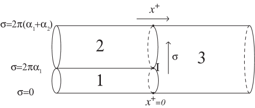
Figure 7: Three string interaction vertex in the light-cone gauge. Note that, due to closed string boundary conditions, $\sigma=0$, $\sigma=2\pi\alpha_{1}$ and $\sigma=2\pi(\alpha_{1}+\alpha_{2})$ are identified and $I$ is the interaction point.

To evaluate the integral (VIII.21) we need to parametrize the interaction vertex from the worldsheet point of view. This has been depicted in Fig. 7. It is convenient to define $\sigma_{r}$ as

$$\sigma_{(1)} = \sigma\ \ \ \ \ \ \ \ \ \ \ 0\leq\sigma\leq 2\pi\alpha_{1}$$ (VIII.24)

$$\sigma_{(2)} = \sigma-2\pi\alpha_{1}\ \ \ \ \ \ \ 2\pi\alpha_{1}\leq\sigma\leq 2\pi(\alpha_{1}+\alpha_{2})$$ (VIII.25)

$$\sigma_{(3)} = -\sigma\ \ \ \ \ \ \ \ \ 0\leq\sigma\leq 2\pi(\alpha_{1}+\alpha_{2})$$

Then in general it should be understood that $P_{(r)}(\sigma)$ is only defined on the domain of $\sigma_{r}$ and otherwise it is zero. As first step we rewrite the $\Delta$-functionals in terms of the Fourier modes, for that we make use of $\Delta[F(\sigma)]=\prod_{n=-\infty}^{\infty}\ \delta\left(\int_{0}^{2\pi|\alpha_{3}|}d\sigma\ e^{in\sigma/|\alpha_{3}|}F(\sigma)\right)$, hence

$$\Delta[P_{(r)}(\sigma)]=\prod_{m=-\infty}^{\infty}\ \delta\left(\sum_{r,n}X^{r}_{mn}p_{n(r)}\right)$$ (VIII.26)

where $X^{3}_{mn}=\delta_{mn}$ and

$$\begin{array}[]{cc}X^{1}_{mn}(\beta)=\frac{2(-1)^{m+n+1}}{\pi}\frac{m\beta\sin\pi m\beta}{n^{2}-m^{2}\beta^{2}}\ ,&\ \ \ \ X^{1}_{m,0}(\beta)=\frac{\sqrt{2}(-1)^{m}}{\pi}\frac{\sin\pi m\beta}{m\beta}\cr\cr X^{1}_{-m,-n}(\beta)=\frac{2(-1)^{m+n+1}}{\pi}\frac{n\sin\pi m\beta}{n^{2}-m^{2}\beta^{2}}\ ,&\ \ \ X^{1}_{0,0}=1\ ,\ \ \ \ X^{1}_{m,n}=0\ \ {\rm otherwise}\ ,\end{array}$$ (VIII.27)

$\beta=\frac{\alpha_{1}}{\alpha_{3}}$ and in (VIII.27) $m,n>0$. Then, $X^{2}_{m,n}$ can be written in terms of $X^{1}$ as $X^{2}_{m,n}(\beta)=(-1)^{n}X^{1}_{m,n}(\beta+1)$ for any $m,n\in\mathbb{Z}$. Using (VIII.10) we can perform the Gaussian momentum integrals of (VIII.21) to obtain the bosonic part of $|V_{3}\rangle$:

$$|E_{a}\rangle={\rm exp}\left[\frac{1}{2}\sum_{r,s=1}^{3}\sum_{m,n\in\mathbb{Z}}\delta^{IJ}a^{I\dagger}_{m(r)}{\overline{N}}^{(rs)}_{mn}a^{J\dagger}_{n(s)}\right]|{\rm v}\rangle_{3}$$ (VIII.28)

where the Neumann matrices ${\overline{N}}^{(rs)}_{mn}$ are given by

$${\overline{N}}^{(rs)}_{mn}=\delta^{rs}\delta_{mn}-2\sqrt{\omega_{m(r)}\omega_{n(s)}}(X^{(r)}\Gamma^{-1}_{a}X^{(s)})_{mn}\ ,$$ (VIII.29)

in which

$$(\Gamma^{-1}_{a})_{mn}=\sum_{r=1}^{3}\sum_{p\in\mathbb{Z}}\omega_{p(r)}X^{(r)}_{mp}X^{(r)}_{pn}\$$

and $\omega_{n(r)}=\sqrt{n^{2}+\mu^{2}\alpha^{2}_{r}}$. Similarly one can work out the fermionic integrals with fermionic Neumann functions ${\overline{Q}}^{(rs)}_{mn}$ Pankiewicz (2003)

$$|E_{b}\rangle={\rm exp}\left[\frac{1}{2}\sum_{r,s=1}^{3}\sum_{m,n\geq 0}(b^{\dagger\alpha\beta}_{-m(r)}b^{\dagger}_{n(s)\alpha\beta}+b^{\dagger\dot{\alpha}\dot{\beta}}_{m(r)}b^{\dagger}_{-n(s)\dot{\alpha}\dot{\beta}}){\overline{Q}}^{(rs)}_{mn}\right]|{\rm v}\rangle_{3}$$ (VIII.30)

(Explicit formulas for ${\overline{Q}}^{(rs)}_{mn}$ and ${\overline{N}}^{(rs)}_{mn}$ can be found in Pankiewicz (2003); He et al. (2003).)

As mentioned earlier (VIII.15a) and a part of (VIII.16) should still be imposed on $|H^{(3)}\rangle$ and $|Q^{(3)}\rangle$. These are nothing but the worldsheet continuity conditions

$$\sum_{r=1}^{3}e(\alpha_{r})X_{(r)}(\sigma)|H^{(3)}\rangle=0,\ \ \ \sum_{r=1}^{3}e(\alpha_{r})\theta^{\alpha\beta}_{(r)}(\sigma)|H^{(3)}\rangle=0,\ \ \ \sum_{r=1}^{3}e(\alpha_{r})\theta^{\dot{\alpha}\dot{\beta}}_{(r)}(\sigma)|H^{(3)}\rangle=0,$$ (VIII.31)

and similarly for $|Q^{(3)}\rangle$. One can show that $|V_{3}\rangle$ already satisfies these conditions Spradlin and Volovich (2002). We would like to comment that the Neumann matrices ${\overline{N}}^{(rs)}_{mn}$ and ${\overline{Q}}^{(rs)}_{mn}$ are invariant under CPT (cf. (II.33)) He et al. (2003); Schwarz (2002).

VIII.2.2 Interaction point operator

In this part we use the dynamical $PSU(2|2)\times PSU(2|2)\times U(1)_{-}$ superalgebra to determine the “prefactors” $H_{3}$ and $Q_{3}$ (cf. (VIII.18) or (VIII.22)). For that we expand both sides of (II.47) and (II.51) in powers of $g_{s}$ and note that the equality should hold at any order in $g_{s}$. At first order in $g_{s}$ we obtain

$$[{\widehat{\cal H}}^{(3)},{\widehat{Q}}^{(0)}_{\alpha\dot{\beta}}]+[{\widehat{\cal H}}^{(2)},{\widehat{Q}}^{(3)}_{\alpha\dot{\beta}}] =0\ ,$$ (VIII.32a)

$$\{{\widehat{Q}}^{(3)}_{\alpha\dot{\beta}},({\widehat{Q}}^{(0)})^{\dagger}_{\rho\dot{\lambda}}\}+\{{\widehat{Q}}^{(0)}_{\alpha\dot{\beta}},({\widehat{Q}}^{(3)})^{\dagger}_{\rho\dot{\lambda}}\} =2\epsilon_{\alpha\rho}\epsilon_{\dot{\beta}\dot{\lambda}}{\widehat{\cal H}}^{(3)}.$$ (VIII.32b)

The equations for ${\widehat{Q}}_{\dot{\alpha}\beta}$ is quite similar and hence we do not present them here. In fact, as in the flat space case, one can show $H_{3}$ and $Q_{3}$ as a function of worldsheet coordinate $\sigma$ should only be non-zero at the interaction point $\sigma=2\pi\alpha_{1}$ Green et al. (1987a) chapter 11. This and the necessity of these prefactors may be seen by first setting $H_{3}=1$ and demanding (VIII.32a) to hold, i.e.

$$\sum_{r=1}^{3}{\widehat{\cal H}}^{(2)}_{r}|Q^{(3)}_{\alpha\dot{\beta}}\rangle+\sum_{r=1}^{3}{\widehat{Q}}^{(0)}_{\alpha\dot{\beta}(r)}|V_{3}\rangle=0\ .$$

Then the conservation of energy at each vertex implies that $\sum_{r=1}^{3}{\widehat{\cal H}}^{(2)}_{r}=0$ for the physical string states (which are necessarily on-shell), and hence the above equation reduces to

$$\sum_{r=1}^{3}\int d\sigma_{r} \biggl{[} (4\pi P^{i}_{(r)}-i\mu X^{i}_{(r)})(\sigma_{i})_{\alpha}^{\ \dot{\rho}}\theta^{\dagger}_{\dot{\rho}\dot{\beta}{(r)}}+(4\pi P^{a}_{(r)}+i\mu X^{a}_{(r)})(\sigma_{a})_{\dot{\beta}}^{\ \rho}\theta^{\dagger}_{\alpha\rho{(r)}}$$ (VIII.33)

$$+ i\partial_{\sigma}X^{i}_{(r)}(\sigma_{i})_{\alpha}^{\ \dot{\rho}}\theta_{\dot{\rho}\dot{\beta}{(r)}}+i\partial_{\sigma}X^{a}_{(r)}(\sigma_{a})_{\dot{\beta}}^{\ \rho}\theta_{\alpha\rho{(r)}}\biggr{]}|V_{3}\rangle=0\ .$$ (VIII.34)

where we have used (IV.54a) for ${Q}^{(0)}$’s. In is easy to check that the integrand of (VIII.33) on $|V_{3}\rangle$ is generically vanishing and the only non-zero contribution comes from the interaction point $\sigma=2\pi\alpha_{1}$. However, at this point the integrand is singular and after integration over $\sigma$ yields a finite result, i.e. (VIII.33) is not satisfied and hence $H_{3}\neq 1$.

To work out $H_{3}$ and $Q_{3}$ we again use the number operator basis and try to solve (VIII.32). These equations in terms of $H_{3}$ and $Q_{3}$ are

$$\sum_{r=1}^{3}\left({\widehat{\cal H}}^{(2)}_{r}{(Q_{3})}_{\alpha\dot{\beta}}+{\widehat{Q}}^{(0)}_{\alpha\dot{\beta}(r)}H_{3}\right)|V_{3}\rangle =0\ ,$$ (VIII.35a)

$$\sum_{r=1}^{3}\left({\widehat{Q}}^{(0)\dagger}_{\alpha\dot{\beta}(r)}{(Q_{3})}_{\rho\dot{\lambda}}+{\widehat{Q}}^{(0)\dagger}_{\rho\dot{\lambda}(r)}{(Q_{3})}_{\alpha\dot{\beta}}\right)|V_{3}\rangle =2\epsilon_{\alpha\rho}\epsilon_{\dot{\beta}\dot{\lambda}}H_{3}|V_{3}\rangle\ .$$ (VIII.35b)

These equations, being linear in $Q_{3}$ and $H_{3}$, only allow us to determine ${\widehat{\cal H}}^{(3)}$ and ${\widehat{Q}}^{(3)}$ up to an overall $\mu$ (or more precisely $\alpha^{\prime}\mu p^{+}$) dependent factor. This should be contrasted with the flat space case, where besides the above there is an extra condition coming from the boost in the light-cone directions (generated by $J^{+-}$ in the notations of section II.3.1) Green et al. (1983). In the plane-wave background, however, this boost symmetry is absent and this overall factor should be fixed in some other way, e.g. by comparing the SFT results by their gauge theory correspondents (which are valid for $\alpha^{\prime}\mu p^{+}\gg 1$) or by the results of supergravity on the plane-wave background (which are trustworthy for $\alpha^{\prime}\mu p^{+}\ll 1$).

First we note that, in order to guarantee the continuity conditions (VIII.15) and (VIII.16), the prefactors should (anti)commute with the kinematical supersymmetry generators. Then, one can show that there exist linear combinations of the bosonic and fermionic creation operators which satisfy these continuity conditions:

$${\cal K}^{I}=\sum_{r=1}^{3}\sum_{n\in\mathbb{Z}}K_{n(r)}a^{I\dagger}_{n(r)}\ ,\ \ \ {\widetilde{\cal K}}^{I}=\sum_{r=1}^{3}\sum_{n\in\mathbb{Z}}{\widetilde{K}}_{n(r)}a^{I\dagger}_{n(r)},\ \ {\widetilde{K}}_{n(r)}=K_{n(r)}^{*}$$ (VIII.36a)

$$Y^{\alpha\beta}=\sum_{r=1}^{3}\sum_{n\geq 0}{\bar{G}}_{n(r)}b^{\dagger\alpha\beta}_{n(r)}\ ,\ \ \ Z^{\dot{\alpha}\dot{\beta}}=\sum_{r=1}^{3}\sum_{n\geq 0}{\bar{G}}_{n(r)}b^{\dagger\dot{\alpha}\dot{\beta}}_{-n(r)}\ ,\ \ \ {\bar{G}}_{n(r)}={\bar{G}}_{n(r)}^{*}.$$ (VIII.36b)

$K_{n(r)},\ {\widetilde{K}}_{n(r)},\ {\bar{G}}_{n(r)}$ have complicated expressions and are functions of $\mu$ and $p^{+}$. Since we do not find their explicit formulas illuminating we do not present them here, however, the interested reader may find them in Spradlin and Volovich (2003c); Pankiewicz (2002); He et al. (2003); Di Vecchia et al. (2003); Pankiewicz (2003). Therefore, taking prefactors to be functions of ${\cal K}^{I},\ {\widetilde{\cal K}}^{I},\ Y^{\alpha\beta}$ and $Z^{\dot{\alpha}\dot{\beta}}$ would guarantee the continuity conditions.

Equipped with (VIII.36) we are ready to solve (VIII.35). Here we only present the results and for more detailed calculations, which are lengthy but straightforward, we refer the reader to Pankiewicz (2003). The main part of the calculation is to work out some number of relations and identities among $K$’s, $Y$’s and $Z$’s.

$$(Q_{3})_{\alpha\dot{\beta}} = e^{i\pi/4}|\alpha_{3}|^{3/2}\sqrt{-\beta(\beta+1)}\left(S^{+}_{\dot{\rho}\dot{\beta}}(Z)T^{+}_{\alpha\lambda}(Y^{2}){\widetilde{\cal K}}_{1}^{\dot{\rho}\lambda}+iS^{+}_{\alpha\lambda}(Y)T^{-}_{\dot{\rho}\dot{\beta}}(\tilde{Z}^{2}){\widetilde{\cal K}}_{2}^{\dot{\rho}\lambda}\right)\times f(\mu)$$ (VIII.37)

$$(Q_{3})_{\dot{\alpha}\beta} = -e^{-i\pi/4}|\alpha_{3}|^{3/2}\sqrt{-\beta(\beta+1)}\left(S^{-}_{\lambda\beta}(Y)T^{-}_{\dot{\alpha}\dot{\rho}}(Z^{2}){\widetilde{\cal K}}_{1}^{\lambda\dot{\rho}}+iS^{-}_{\dot{\alpha}\dot{\rho}}(Z)T^{+}_{\lambda\beta}(\tilde{Y}^{2}){\widetilde{\cal K}}_{2}^{\lambda\dot{\rho}}\right)\times f(\mu)$$ (VIII.38)

$$H_{3} = \biggl{[}\left({\cal K}^{i}{\widetilde{\cal K}}^{j}+\frac{\mu\beta(\beta+1)}{2}\alpha_{3}^{3}\delta^{ij}\right)V_{ij}-\left({\cal K}^{a}{\widetilde{\cal K}}^{b}+\frac{\mu\beta(\beta+1)}{2}\alpha_{3}^{3}\delta^{ab}\right)V_{ab}$$ (VIII.39)

$$- {\cal K}_{1}^{\dot{\alpha}\rho}{\widetilde{\cal K}}_{2}^{\dot{\beta}\lambda}S^{+}_{\rho\lambda}(Y)S^{-}_{\dot{\alpha}\dot{\beta}}(Z)-{\widetilde{\cal K}}_{1}^{\dot{\alpha}\rho}{\cal K}_{2}^{\dot{\beta}\lambda}S^{-}_{\rho\lambda}(Y)S^{+}_{\dot{\alpha}\dot{\beta}}(Z)\biggr{]}\times f(\mu)$$ (VIII.40)

where $\beta=\frac{\alpha_{1}}{\alpha_{3}},\ |\alpha_{3}|=\alpha^{\prime}p^{+}$ (note that in our conventions $\alpha_{3}<0$ and $-1\leq\beta<0$) and

$${\widetilde{\cal K}}_{1}^{\dot{\alpha}\rho}\equiv{\widetilde{\cal K}}^{i}{(\sigma_{i})}^{\dot{\alpha}\rho}\ ,\ \ \ {{\cal K}}_{1}^{\dot{\alpha}\rho}\equiv{{\cal K}}^{i}{(\sigma_{i})}^{\dot{\alpha}\rho} \ \ {\widetilde{\cal K}}_{2}^{\dot{\alpha}\rho}\equiv{\widetilde{\cal K}}^{a}{(\sigma_{a})}^{\dot{\alpha}\rho}\ ,\ \ \ {{\cal K}}_{2}^{\dot{\alpha}\rho}\equiv{{\cal K}}^{a}{(\sigma_{a})}^{\dot{\alpha}\rho}\ ,\ \ \$$ , (VIII.41)

$$S^{\pm}(Y)=Y\pm\frac{i}{3}Y^{3}\ \ \ \ T^{\pm}(Z^{2})=\epsilon\pm{i}Z^{2}-\frac{1}{6}Z^{4}\ ,$$ , (VIII.42)

$$V_{ij}=\delta_{ij}\left[1+\frac{1}{12}(Y^{4}+Z^{4})+\frac{1}{144}Y^{4}Z^{4}\right] - \frac{i}{2}\left[Y^{2}_{ij}(1+Z^{4})-Z^{2}_{ij}(1+\frac{1}{12}Y^{4})\right]+\frac{1}{4}(Y^{2}Z^{2})_{ij}$$ (VIII.43)

$$V_{ab}=\delta_{ab}\left[1-\frac{1}{12}(Y^{4}+Z^{4})+\frac{1}{144}Y^{4}Z^{4}\right] - \frac{i}{2}\left[Y^{2}_{ab}(1-Z^{4})-Z^{2}_{ab}(1-\frac{1}{12}Y^{4})\right]+\frac{1}{4}(Y^{2}Z^{2})_{ab}$$ (VIII.44)

In the above,

$$Y^{2}_{\alpha\beta}\equiv Y_{\alpha\rho}Y_{\beta}^{\ \rho},\ \ \ {\tilde{Y}}^{2}_{\alpha\beta}\equiv Y_{\rho\alpha}Y^{\rho}_{\ \beta}\ ,\ \ \ Y^{4}_{\alpha\beta} \equiv Y^{2}_{\alpha\rho}(Y^{2})_{\beta}^{\ \rho}=\frac{-1}{2}\epsilon_{\alpha\beta}Y^{4}\ ,\ \ \ \tilde{Y}^{4}_{\alpha\beta}\equiv\tilde{Y}^{2}_{\alpha\rho}(\tilde{Y}^{2})_{\beta}^{\ \rho}=\frac{1}{2}\epsilon_{\alpha\beta}Y^{4}\ ,$$ (VIII.45)

$$Y^{3}_{\alpha\beta}\equiv Y_{\alpha\rho}Y^{\lambda\rho}Y_{\lambda\beta},\ \ \ Y^{2}_{ij}=(\sigma_{ij})^{\alpha\beta}Y^{2}_{\alpha\beta} \ \ Z^{2}_{ij}=(\sigma_{ij})^{\dot{\alpha}\dot{\beta}}Z^{2}_{\dot{\alpha}\dot{\beta}}\ ,\ \ \ (Y^{2}Z^{2})_{ij}=Y^{2}_{k(i}Z^{2}_{j)k}\ ,$$ ,

where $Y^{4}\equiv Y^{2}_{\alpha\beta}{(Y^{2})}^{\alpha\beta}=-{\tilde{Y}}^{2}_{\alpha\beta}{({\tilde{Y}}^{2})}^{\alpha\beta}$. Note that $Y^{2}$, ${\tilde{Y}}^{2}$ (and similarly $Z_{\dot{\alpha}\dot{\beta}}^{2},\ \tilde{Z}_{\dot{\alpha}\dot{\beta}}^{2}$) are symmetric matrices, i.e. both of their indices belong to only one of $SO(4)$’s; in fact $Y^{2}$ and $Z^{2}$ are matrices in the first $SO(4)$ and ${\tilde{Y}}^{2}$ and $\tilde{Z}^{2}$ in the second one, moreover $V_{ij}$ and $V_{ab}$ are Hermitian, $V_{ij}^{*}=V_{ji}$ and $V_{ab}^{*}=V_{ba}$. The function $f(\mu)$ (or more precisely $f(\alpha^{\prime}\mu p^{+})$) is an overall factor which is not fixed through the superalgebra requirements (cf. discussions following (VIII.35)).

In order to have a better sense of the above it is instructive to consider the bosonic case. This can be done by setting $Y$ and $Z$ equal to zero (and hence $V_{ij}=\delta_{ij}$ and $V_{ab}=\delta_{ab}$). This would considerably simplify (VIII.40) and we obtain

$$|H^{(3)}\rangle = f(\mu)({\cal K}_{i}{\widetilde{\cal K}}_{i}-{\cal K}_{a}{\widetilde{\cal K}}_{a})|E_{a}\rangle\delta(\sum_{r=1}^{3}\alpha_{r})$$ (VIII.46)

$$= \frac{f(\mu)}{4\pi}|\alpha_{3}|^{3}\beta(\beta+1)\sum_{r=1}^{3}\sum_{n\in\mathbb{Z}}\frac{\omega_{n(r)}}{\alpha_{r}}(a^{i\dagger}_{n(r)}a^{i}_{-n(r)}-a^{a\dagger}_{n(r)}a^{a}_{-n(r)})|E_{a}\rangle\delta(\sum_{r=1}^{3}\alpha_{r})\ ,$$ (VIII.47)

where $\omega_{n(r)}=\sqrt{n^{2}+\mu^{2}\alpha_{r}^{2}}$. To obtain the second line, some identities among $K_{n(r)}$ have been employed Lee et al. (2003); Pearson et al. (2003). We would like to note the $\mathbb{Z}_{2}$ behaviour of $|H^{(3)}\rangle$. This $\mathbb{Z}_{2}$, as discussed in section II.3.1 exchanges the two $SO(4)$’s of $SO(4)\times SO(4)$ isometry. From (VIII.46) it is evident that ${\cal K}_{i}{\widetilde{\cal K}}_{i}-{\cal K}_{a}{\widetilde{\cal K}}_{a}$ is odd under $\mathbb{Z}_{2}$. However, as we argued (cf. section IV.3) the vacuum $|{\rm v}\rangle$ is odd under $\mathbb{Z}_{2}$, therefore altogether $|H^{(3)}\rangle$ is $\mathbb{Z}_{2}$ even. Of course with a little bit of work, one can show that this property is also true for the full expression of (VIII.40).

Before closing this subsection we should warn the reader that in the most of the plane-wave SFT literature (e.g. Spradlin and Volovich (2002); Spradlin and Volovich (2003c)) $SO(8)$ fermionic representations together with an $SO(8)$ invariant vacuum $|0\rangle$ or $|\dot{0}\rangle$ (cf. (IV.42)) have been used. In the $SO(8)$ notation, unlike our case, this $\mathbb{Z}_{2}$ symmetry is not manifest. It has been shown that the $SO(4)\times SO(4)$ formulation we presented here and the $SO(8)$ one are indeed equivalent Pankiewicz and Stefanski (2003a). In the $SO(8)$ notation it is very easy to observe that, as one would expect, in the $\mu\to 0$ limit goes over to the well-known flat space result; this point can be (and in fact have been) used as a cross check for the calculations.

VIII.3 Plane-wave light-cone SFT contact terms

In this section we will test the plane-wave/SYM duality at ${\cal O}(g_{2}^{2})$ by working out the one-loop corrections to single-string spectrum. Explicitly, we run the machinery of quantum mechanical time independent perturbation theory with the Hilbert space ${\mathbb{H}}$ and Hamiltonian ${\widehat{\cal H}}$. One might also try to use time dependent perturbation theory starting with string wave-packets to study strings scattering processes, the point which will not be studied here and we will only make some comments about that later on in this section and also in section IX.

It is easy to see that at first order in $g_{s}$ time independent perturbation theory gives a vanishing result for energy shifts, i.e. $\langle\psi|{\widehat{\cal H}}^{(3)}|\psi\rangle=0$ for any $|\psi\rangle\in{\mathbb{H}}_{1}$ (of course one should consider degenerate perturbation theory, nevertheless this result is obviously still true). Therefore we should consider the second order corrections. For that, however, we need to work out ${\widehat{\cal H}}^{(4)}$. So, in this section first we will continue the analysis of section VIII.2 and work out the needed parts of ${\widehat{\cal H}}^{(4)}$. As we will see, to compare the gauge theory results of section VII against the string (field) theory side we do not need to have the full expression of ${\widehat{\cal H}}^{(4)}$, which considerably simplifies the calculation.

VIII.3.1 Four string vertices

The procedure of finding ${\widehat{\cal H}}^{(4)}$ and ${\widehat{Q}}^{(4)}$ is essentially a direct continuation of the lines of previous section; i.e. solving the continuity conditions (VIII.15), (VIII.16) and (VIII.17) together with the constraints coming from the dynamical supersymmetry algebra, which are

$$[{\widehat{\cal H}}^{(3)},{\widehat{Q}}^{(3)}_{\alpha\dot{\beta}}]+[{\widehat{\cal H}}^{(2)},{\widehat{Q}}^{(4)}_{\alpha\dot{\beta}}]+[{\widehat{\cal H}}^{(4)},{\widehat{Q}}^{(0)}_{\alpha\dot{\beta}}] =0\ ,$$ (VIII.48a)

$$\{{\widehat{Q}}^{(3)}_{\alpha\dot{\beta}},({\widehat{Q}}^{(3)})^{\dagger}_{\rho\dot{\lambda}}\}+\{{\widehat{Q}}^{(0)}_{\alpha\dot{\beta}},({\widehat{Q}}^{(4)})^{\dagger}_{\rho\dot{\lambda}}\}+\{{\widehat{Q}}^{(4)}_{\alpha\dot{\beta}},({\widehat{Q}}^{(0)})^{\dagger}_{\rho\dot{\lambda}}\} =2\epsilon_{\alpha\rho}\epsilon_{\dot{\beta}\dot{\lambda}}{\widehat{\cal H}}^{(4)}.$$ (VIII.48b)

The important point to be noted is that ${\widehat{\cal H}}^{(4)}$ contains two essentially different pieces, one is the part which does not change the string number and the other is the part which changes string number by two (cf. (VIII.14b)). In fact in our analysis to find mass corrections to single-string states we need to calculate $\langle\psi|{\widehat{\cal H}}^{(4)}|\psi\rangle,\ \ |\psi\rangle\in\mathbb{H}_{1}$. We then note that ${\widehat{Q}}^{(4)}$ is quartic in string field $\Phi$ and that ${\widehat{Q}}^{(0)}$ maps $\mathbb{H}_{1}$ onto $\mathbb{H}_{1}$. Therefore the terms in (VIII.48b) involving ${\widehat{Q}}^{(4)}$ do not contribute to energy shift of single-string states at the $g_{s}^{2}$ level. This in particular means that we need not calculate ${\widehat{Q}}^{(4)}$ and therefore we have all the necessary ingredients for calculating the one-loop string corrections to the strings mass spectrum.

VIII.3.2 One-loop corrections to string spectrum

In this subsection we compute the mass shift to the string state in $({\bf 9},{\bf 1})$ representation of $SO(4)\times SO(4)$ (cf. section IV.3), i.e.

$$|(ij),\ n\rangle\equiv\frac{1}{\sqrt{2}}\alpha^{(i\dagger}_{n}\tilde{\alpha}^{j)\dagger}_{n}|{\rm v}\rangle=\frac{1}{\sqrt{2}}(\alpha^{i\dagger}_{n}\tilde{\alpha}^{j\dagger}_{n}+\alpha^{j\dagger}_{n}\tilde{\alpha}^{i\dagger}_{n}-\frac{1}{2}\delta^{ij}\alpha^{k\dagger}_{n}\tilde{\alpha}^{k\dagger}_{n})|{\rm v}\rangle\ ,$$ (VIII.49)

where it is easy to show that

$$\langle(kl),\ m|(ij),\ n\rangle\equiv\delta_{mn}T^{ijkl}=\delta_{mn}(\delta^{ik}\delta^{jl}+\delta^{il}\delta^{jk}-\frac{1}{2}\delta^{ij}\delta^{kl})\ .$$ (VIII.50)

The computation for the mass shift should, in principle, be repeated for all the string states in different $SO(4)\times SO(4)$ representations discussed in IV.3. However, we only present that of $({\bf 9},{\bf 1})$. Noting that the states with the same excitation number $n$, but with different $SO(4)\times SO(4)$ representations are generically related by the plane-wave superalgebra (cf. section II.3) and also the fact that we have constructed the $g_{s}$ correction to light-cone SFT so that they respect the same supersymmetry algebra, imply that the mass shifts for these states should only depend on the excitation number $n$ and not the details of their $SO(4)\times SO(4)$ representation. In more precise terms, in the $PSU(2|2)\times PSU(2|2)\times U(1)_{-}$ superalgebra the Hamiltonian commutes with the supercharges (II.47) implying that all the states in the same $PSU(2|2)\times PSU(2|2)\times U(1)_{-}$ supermultiplet should necessarily have the same mass for any value of string coupling. On the other hand it is easy to show that all the states presented in (IV.43) and (IV.44) form a (long) multiplet of this algebra specified with one single quantum number, $n$. (Of course there is another physical number which is not encoded in the superalgebra representations, the string number or from the BMN gauge theory point of view the number of traces in the BMN operators.) This result have also been checked through explicit one-loop SFT calculations for $({\bf 1},{\bf 1})$ Gomis et al. (2003b), for $({\bf 3}^{\pm},{\bf 1})$ Roiban et al. (2002) and for $({\bf 4},{\bf 4})$ Pankiewicz (2003).

The corrections to the mass at order $g_{s}^{2}$ receives contributions from second order perturbation theory with ${\widehat{\cal H}}^{(3)}$ and first order perturbation with ${\widehat{\cal H}}^{(4)}$:

$$\delta E_{n}^{(2)}=g_{s}^{2}\left(\sum_{1,2\in{\mathbb{H}}_{2}}\frac{1}{2}\frac{|\langle 1,2|{\widehat{\cal H}}^{(3)}|(ij),n\rangle|^{2}}{E^{(0)}_{n}-E_{1,2}^{(0)}}+\frac{1}{8}\langle(ij),n|\{{\widehat{Q}}^{(3)}_{\alpha\dot{\beta}},{\widehat{Q}}^{(3)\dagger\alpha\dot{\beta}}\}|(ij),n\rangle\right)\ .$$ (VIII.51)

The extra $\frac{1}{2}$ factor in the first term comes from the fact that this term arises from a second order perturbation theory $\left({\rm e}^{S+\delta S}={\rm e}^{S}(1+\delta S+\frac{1}{2}(\delta S)^{2}\right)$ or in other words it is due to the reflection symmetry of the one-loop light-cone string diagram Roiban et al. (2002) while $\frac{1}{8}$ factor in the second term is obtained noting (VIII.48b) after taking the trace over $\alpha\rho$ and $\dot{\beta}\dot{\lambda}$ indices. Note that since the Hamiltonian is a singlet of $SO(4)\times SO(4)\rtimes\mathbb{Z}_{2}$ and also following our superalgebra arguments, we expect states in different irreducible $SO(4)\times SO(4)$ representations not to mix and hence we use non-degenerate perturbation theory.

To evaluate the right-hand side of (VIII.51) we note that since ${\widehat{Q}}^{(3)}_{\alpha\dot{\beta}}$ is cubic in string fields the second term can be written as

$$\frac{1}{8}\langle(ij),n|\{{\widehat{Q}}^{(3)}_{\alpha\dot{\beta}},{\widehat{Q}}^{(3)\dagger\alpha\dot{\beta}}\}|(ij),n\rangle=\frac{1}{4}\sum_{1,2\in{\mathbb{H}}_{2}}\langle(ij),n|{\widehat{Q}}^{(3)}_{\alpha\dot{\beta}}|1,2\rangle\langle 1,2|{\widehat{Q}}^{(3)\dagger\alpha\dot{\beta}}|(ij),n\rangle.$$

Next we note that the light-cone momentum $p^{+}$ ($\alpha_{3}$ in the notation of section VIII.2) can be distributed among the “internal” states $|1,2\rangle$ as $\beta=\frac{\alpha_{1}}{\alpha_{3}}$ and $-(\beta+1)=\frac{\alpha_{2}}{\alpha_{3}}$, and then the sum over $1,2\in\mathbb{H}_{2}$ would reduce to a sum over only string excitation modes together with an integral over $\beta$, explicitly

$$\delta E_{n}^{(2)}=-g_{s}^{2}\int_{-1}^{0}\frac{d\beta}{\beta(\beta+1)}\sum_{\begin{array}[]{cc}&{\rm stringy}\\ &{\rm modes}\end{array}}\left(\frac{1}{2}\frac{|\langle 1,2|{\widehat{\cal H}}^{(3)}|(ij),n\rangle|^{2}}{E^{(0)}_{n}-E_{1,2}^{(0)}}+\frac{1}{4}|\langle(ij),n|{\widehat{Q}}^{(3)}_{\alpha\dot{\beta}}|1,2\rangle|^{2}\right)\ .$$ (VIII.52)

The $\frac{1}{\beta}$ and $\frac{1}{\beta+1}$ factors may be understood as the “propagator” of the $1,2$ states in the light-cone or equivalently they arise from the normalization of $1,2$ states indicating the length conservation in the $\sigma$ direction (this may be put in other words: the light-cone Hamiltonian $P^{-}$ and the contribution of the transverse momenta to energy differ by a factor of $\frac{1}{p^{+}}$ Bak and Sheikh-Jabbari (2003)).

Let us first spell out the steps of performing the calculations and work out the necessary ingredients:

$\bullet$ 0) Since in the plane-wave background $P^{+}$ commutes with all the other supersymmetry generators we can always restrict ourselves to a sector with a given $p^{+}$ (this is to be contrasted with the flat space case where $J^{+-}$ and $J^{-I}$, which are absent in the plane-wave case, can change $p^{+}$). Therefore, instead of the dimensionless parameter $\alpha^{\prime}\mu p^{+}$ in our calculations without any ambiguity we will simply use $\mu$. For example $\lambda^{\prime}$ expansion in the gauge theory side would correspond to large $\mu$ expansion (cf. (I.11)) on the SFT side.

$\bullet$ i) In the gauge theory calculations of section VII we diagonalized the dilatation operator only in a subspace of the BMN operators, the sector which had the same number of impurities, i.e. the impurity conserving sector. Although this truncation was not physically strongly justified, for the matter of comparison, in the SFT calculations only the same subsector must be included. Explicitly, in the sum over the two string states in (VIII.52) only the string states with two stringy excitations (one left and one right mover) should be included. We will have more discussion on this point later on in this section.

$\bullet$ ii) Noting that $|(ij),n\rangle$, defined in (VIII.49), is in $({\bf 9},{\bf 1})$ and ${\widehat{\cal H}}^{(3)}$ a singlet of $SO(4)\times SO(4)$, in the first term of (VIII.52) only $|1\rangle\otimes|2\rangle$ states which are in $({\bf 9},{\bf 1})$ representation would contribute and as discussed in section IV.3.1 this state should necessarily be in the “NSNS” sector. This in particular implies that fermionic modes (i.e. “RR” modes) do not contribute to the first term of (VIII.52) and hence to evaluate this term we can simply use (VIII.46).

$\bullet$ iii) Since ${\widehat{Q}}^{(3)}$ is in $({\bf(2,1)},{\bf(1,2)})$ of $SO(4)\times SO(4)$ only the $|1\rangle\otimes|2\rangle$ states in $({\bf 4},{\bf 1})\otimes({\bf(1,2)},{\bf(1,2)})$ representation (which is of course an “RNS” state, cf. section IV.3.1) would contribute.

$\bullet$ iv) The gauge theory results of section VII are at first order in $\lambda^{\prime}$ and this expansion is valid for $\lambda^{\prime}\ll 1$. Therefore the SFT results to be compared with, should be calculated in the corresponding limit, the large $\mu$ limit (cf. (I.11)). The large $\mu$ expansion of the bosonic Neumann functions which would appear in our calculations are Spradlin and Volovich (2003c)

$${\overline{N}}^{(r3)}_{mn}(\beta)=-\sqrt{-\frac{\alpha_{r}}{\alpha_{3}}}X^{r}_{nm}(\beta)+{\cal O}(\mu^{-2}),\ \ r\in\{1,2\},\ m,n\in\mathbb{Z}\ ,$$ (VIII.53)

where $X^{r}_{nm}$ is given in (VIII.27).

$\bullet$ v) As stated above, $|1,2\rangle$ states contributing to the first term of the sum (VIII.52) in the impurity conserving sector should be of the form $|(kl),\ m\rangle_{\alpha_{2}}\otimes|{\rm v}\rangle_{\alpha_{1}}$ or $\alpha^{(k\dagger}_{0(r)}|{\rm v}\rangle_{\alpha_{1}}\otimes\alpha^{l)\dagger}|{\rm v}\rangle_{\alpha_{2}}$ where the index $\alpha_{r}$ indicates the portion of the light-cone momentum carried by that state. Noting the form of $|H^{(3)}\rangle$ given in (VIII.46) we observe that the non-zero contribution to ${}_{\alpha_{3}}\langle(ij),n|\otimes_{\alpha_{2}}\langle(kl),m|\otimes_{\alpha_{1}}\langle{\rm v}||H^{(3)}\rangle$ should be proportional to $({\overline{N}}^{(r3)})^{2}$ because ${}_{\alpha_{3}}\langle(ij),n|\otimes_{\alpha_{2}}\langle(kl),m|\otimes_{\alpha_{1}}\langle{\rm v}|$ contains four stringy annihilation operators and the prefactor of $|H^{(3)}\rangle$ has another one, hence we need to pick the term which contains five creation operators. This implies that the exponential of (VIII.28) should be expanded to second order. Performing the calculations and using the identities Roiban et al. (2002)

$$\sum_{p\geq 0}{\overline{N}}^{(r3)}_{\pm m,\pm p}{\overline{N}}^{(r3)}_{\pm n,\pm p}=-\frac{(-1)^{m+n}\delta_{r,1}+\delta_{r,2}}{\pi}\left[\frac{\sin(\pi(n-m)\beta)}{n-m}\pm\frac{\sin(\pi(n+m)\beta)}{n+m}\right],\ \ \ \ m,n>0$$

we find that Spradlin and Volovich (2003c); Roiban et al. (2002)

$$\langle{\rm v}|\alpha^{(i\dagger}_{n(3)}\tilde{\alpha}^{j)\dagger}_{n(3)}\alpha^{(k\dagger}_{0(r)}\tilde{\alpha}^{l)\dagger}_{0(s)}|H^{(3)}\rangle =\frac{g_{s}f(\mu)}{2\pi^{2}\mu\alpha_{3}^{2}}(\delta^{rs}+\frac{\sqrt{\alpha_{r}\alpha_{s}}}{\alpha_{3}})\sin^{2}n\pi\beta\ T^{ijkl}+{\cal O}(\mu^{-2})\$$ (VIII.54a)

$$\langle{\rm v}|\alpha^{(i\dagger}_{n(3)}\tilde{\alpha}^{j)\dagger}_{n(3)}\alpha^{(k\dagger}_{m(r)}\tilde{\alpha}^{l)\dagger}_{m(r)}|H^{(3)}\rangle =\frac{g_{s}f(\mu)}{2\pi^{2}\mu\alpha_{3}\alpha_{r}}\beta(\beta+1)\sin^{2}n\pi\beta\ T^{ijkl}+{\cal O}(\mu^{-2})\ .$$ (VIII.54b)

These two matrix elements should be compared to their gauge theory correspondents given (VII.33), in which $r\to-\beta$. As we see there is a perfect match if we remember that light-cone string states are normalized to their light-cone momentum, explicitly (VIII.54) equals to those in (VII.33) multiplied with $\sqrt{Jr(1-r)}$. Inserting (VIII.54) into (VIII.52) and performing the $\beta$ integral as well as the sum over $m$ the first term of (VIII.52) is obtained to be

$$\delta E^{(2,1)}_{n}=\mu\frac{\lambda^{\prime}g_{2}^{2}}{4\pi^{2}}\left(\frac{f(\mu)}{2\pi\mu^{2}\alpha^{2}_{3}}\right)\frac{15}{16\pi^{2}n^{2}}\ ,$$ (VIII.55)

where $g_{2}$ is defined in (I.12).

$\bullet$ vi) Similarly one can work out the contributions from the ${\widehat{Q}}^{(3)}$ term. Here we only present the result and for more details the reader is referred to Roiban et al. (2002); Pankiewicz (2003)

$$\delta E^{(2,2)}_{n}=\mu\frac{\lambda^{\prime}g_{2}^{2}}{4\pi^{2}}\left(\frac{f(\mu)}{2\pi\mu^{2}\alpha_{3}^{2}}\right)(\frac{1}{24}+\frac{5}{64\pi^{2}n^{2}})\ .$$ (VIII.56)

Now we can put all the above together. The one-loop contribution to single-string mass spectrum is the sum of (VIII.55) and (VIII.56):

$$\delta E^{(2)}_{n}=\mu\frac{\lambda^{\prime}g_{2}^{2}}{4\pi^{2}}\left(\frac{f(\mu)}{2\pi\mu^{2}\alpha^{2}_{3}}\right)(\frac{1}{12}+\frac{35}{32\pi^{2}n^{2}}).$$ (VIII.57)

Choosing $f(\mu)=2\pi\mu^{2}\alpha^{2}_{3}$ for large $\mu$, this result is in precise agreement with the gauge theory result of (VII.34). In fact it is possible to absorb $f(\mu)$ into $g_{s}$, the SFT expansion parameter, i.e. the effective string coupling is

$$g_{s}^{eff}=g_{s}f(\alpha^{\prime}\mu p^{+})\sim g_{s}(\alpha^{\prime}\mu p^{+})^{2}=g_{2}^{2}$$ (VIII.58)

where $\sim$ in the above shows the large $\mu$ limit.

VIII.3.3 Discussion of the SFT one-loop result

Here we would like to briefly discuss some of the issues regarding the large $\mu$ expansion and the SFT one-loop result (VIII.57). As we discussed (VIII.57) has been obtained by only allowing the “impurity conserving” intermediate string states in the sums (VIII.52). However, at the same order one can have contributions from string states which change impurity by two. For the impurity non-conserving channel the matrix elements of the first term of (VIII.52) are of order $\mu^{2}$ while they are of order $\mu$ in the impurity conserving channel Spradlin and Volovich (2003c, a). Moreover, the energy difference denominator in the impurity changing channel is of order $\mu$ while it is of order $\mu^{-1}$ in the impurity conserving channel. Therefore, altogether the contributions of the impurity conserving and impurity non-conserving channels are of the same order and from the string theory side it is quite natural to consider both of them. However, the available gauge theory calculations are only in the impurity conserving channel; this remains an open problem to tackle.

The other point which should be taken with a grain of salt is the large $\mu$ expansion. In fact as we see in (VIII.52) sums contain energy excitations ranging from zero to infinity. On the other hand to obtain the large $\mu$ expansion generically it is assumed that $\omega_{n}=\sqrt{n^{2}+(\alpha^{\prime}\mu p^{+})^{2}}$ can be expanded as $\alpha^{\prime}\mu p^{+}+\frac{n^{2}}{\alpha^{\prime}\mu p^{+}}+\cdots$; this expansion is obviously problematic when $n$ is very large. In other words the large $\mu$ expansion and the sum over $n$ do not commute. In fact it has been shown that if we do the large $\mu$ expansion first, we will get contributions which are linearly divergent (they grow like $\mu$) Roiban et al. (2002), leading to energy corrections of the order $\mu g^{2}_{2}\sqrt{\lambda^{\prime}}$. However, if we did the sum first and then perform the large $\mu$ expansion, we would get a finite result for any finite value of $\mu$. This is expected if the results are going to reproduce the flat space results in the $\mu\to 0$ limit. This divergent result from the gauge theory point of view, being proportional to $\sqrt{\lambda^{\prime}}$, seems like a non-perturbative effect Klebanov et al. (2002); Spradlin and Volovich (2003a).

IX Concluding remarks and open questions

In this review we presented a new version of the string/gauge theory correspondence, the plane-wave/SYM duality, and spelled out the correspondence between various parameters and quantities on the two sides. As evidence for this duality we reviewed the gauge theory calculations leading to the spectrum of free strings on the plane-wave as well as one-loop corrections to this spectrum, showing strong support for the duality. There have been many other related directions pursued in the literature, and although being interesting in their own turn, they went beyond the scope of a pedagogical review. However, we would like to mention some of these topics:

• Holography in the plane-wave background OR what is the gauge theory whose ’t Hooft strings are type IIB strings on the plane-wave background?

  As a descendent of the AdS/CFT duality, one may wonder if the plane-wave/SYM duality is also holographic. The first and (following AdS/CFT logic) natural guess for the dual theory is a gauge theoryresiding on the boundary of the plane-wave background, which is a one dimensional light-like direction (cf. section II.1). This implies that the holographic dual of strings on the plane-wave background is a quantum mechanical model. Although there have been many attempts in this direction (e.g.see Das et al. (2002); Kiritsis and Pioline (2002); Leigh et al. (2002); Dobashi et al. (2003); Siopsis (2002); Yoneya (2003)), a widely accepted holographic model is still lacking.

• Plane-wave/SYM for open strings

  The plane-wave/SYM duality we discussed in this review was constructed for (type IIB) closed strings. The extension of the duality to the case of open strings has been studied and may be found for e.g. in Berenstein et al. (2002a); Gomis et al. (2003a); Imamura (2003); Lee and Park (2003); Stefanski (2003); Skenderis and Taylor (2003).

• Flat space limit

  In the plane-wave/SYM correspondence, the perturbative gauge theory calculations are only possible at large $\mu$ while the supergravity description of the string theory side can only be trusted for small $\mu$, where the gauge theory is strongly coupled. Since in the $\mu\to 0$ limit the plane-wave background reduces to flat space, one may wonder if it is possible to take the same limit on the gauge theory side and finally obtain a gauge theory description of strings on flat space. This, of course, amounts to knowing about the (non-perturbative) finite $\mu$ behaviour of the BMN gauge theory. It is conceivable that at finite $\mu$ non-perturbative objects such as instantons and D-branes would dominate the dynamics (at least in some corners of the moduli space). Presumably the $\mu\to 0$ limit is not a smooth one and we lose some of the normalizable states of the Hilbert space. This line of questions remains open and should be addressed.

• String bit model and Quantum Mechanical model for BMN gauge theory

  In the large $\mu$ limit one can readily observe that in (IV.7) we can drop the $(\partial_{\sigma}X)^{2}$ term against the mass term $\mu^{2}X^{2}$. This in particular implies that in such a limit strings effectively become a collection of some number of massive particles, the string bits. Hence it is quite natural to expect the large $\mu$ dynamics of strings on the plane-wave background to be governed by a string bit model Verlinde (2002); Vaman and Verlinde (2002); Zhou (2003) in which the effects of string tension and interactions are introduced as interaction terms in the string bit Lagrangian. The proposed string bit model consists of $J$ string bits of mass $\mu$, with the permutation symmetry and more importantly, the $PSU(2|2)\times PSU(2|2)\times U(1)_{-}$ symmetry built into the model. The action for the string bit model, besides the kinetic (quadratic) term, has cubic and quartic terms, but terminates at the quartic level, as dictated by supersymmetry. The model has been constructed (or engineered) so that it gives the free-string mass spectrum. Remarkably it also reproduces the one-loop results of section VII or VIII. Based on this model it has been conjectured that Pearson et al. (2003); Vaman and Verlinde (2002) the “mixing” between the two impurity BMN states, to all orders in $g_{2}$, is given by $|\tilde{\psi}\rangle={\rm e}^{-\frac{g_{2}}{2}{\widehat{\Sigma}}}|\psi\rangle$ and where the operator ${\widehat{\Sigma}}$ is defined as

  $${\widehat{\Sigma}}{\cal O}_{ij,\ n}^{J}=\sum_{r,m}M_{nm}^{r}{\cal T}_{ij,\ m}^{J,r}-\sum_{r}M_{n}^{r}{\cal T}_{ij}^{J,r},$$

  where $M_{nm}^{r}$ and $M_{n}^{r}$ are matrix elements of $\mathcal{U}^{(1)}$ defined in section VII.3. Moreover, one of the basic predictions of the string bit model is that the genus counting parameter $g_{2}$ would always appear through the combination $\lambda^{\prime}g_{2}^{2}$ (cf. (I.13)). This result, however, has been challenged by yet another quantum mechanical model of the BMN gauge theory constructed to capture the dynamics of BMN operators. The Hamiltonain for this quantum mechanical model is the dilatation operator of the ${\cal N}=4$ SYM and its Hilbert space is the BMN states with two impurities Eynard and Kristjansen (2002); Beisert et al. (2003c); Spradlin and Volovich (2003b); Kristjansen (2003). Based on this model it has been argued that there are $\lambda^{\prime}g_{2}^{4}$ corrections to the string mass spectrum at genus two Beisert et al. (2003c), where they also conjectured that to all orders, both in $\lambda^{\prime}$ and $g_{2}^{2}$, the string spectrum is given by the eigenvalues of a “full” Hamiltonian of the form Spradlin and Volovich (2003b); Beisert et al. (2003c)

  $$H_{\rm full}=2\mu\sqrt{1+\lambda^{\prime}H}\,,$$

  and where

  $$H=H_{0}+\frac{1}{2}g_{2}(V+V^{\dagger})+\frac{1}{8}g_{2}^{2}[{\widehat{\Sigma}},V-V^{\dagger}]\,.$$

  Here $V$ is fixed by the requirement of supersymmetry and is such that at $g_{2}=0$ it gives the free-string spectrum and reproduces the one-loop result of (VIII.57). This conjecture has so far passed ${\cal O}(\lambda^{\prime})$ (including $\lambda^{\prime 2}$) tests when compared to the direct gauge theory calculations. However, already a mismatch with the exact SFT results He et al. (2003) has been reported Spradlin and Volovich (2003b). It has been speculated that this mismatch is due to the basic assumption in this quantum mechanical model, where only the two impurity BMN states i.e., the impurity preserving sector (cf. discussion of section VIII.3) has been considered Spradlin and Volovich (2003b). It would be desirable to directly obtain the plane-wave light-cone SFT from the study of BMN gauge theory, some step in this direction has been taken in de Mello Koch et al. (2002, 2003).

• Spectrum of dilatation operator

  According to the plane-wave/SYM duality the dilatation operator should be identified with the light-cone string field theory Hamiltonian. As an alternative way to study and verify this duality one may choose to focus only on the representation of the dilatation operator $\widehat{\cal D}$ on the space of all possible (gauge invariant) operators of the ${\cal N}=4$ SYM theory in the BMN sector. (Note that $\widehat{\cal D}$ is the Hamiltonian of ${\cal N}=4$ SYM theory in the radial quantization.) Therefore, working out $\widehat{\cal D}$ and its spectrum (in powers of the genus counting parameter) would help to establish the BMN duality, as well as solving the full ${\cal N}=4$ SYM theory. This direction of study has recently attracted some attention with a view to solving the full gauge theory, see for e.g. Beisert et al. (2003d); Beisert (2003b); Dolan et al. (2003); Beisert and Staudacher (2003); Beisert et al. (2003e); Belitsky et al. (2003).

• String interactions and scattering

  In section VIII, we worked out in detail the cubic string interaction terms in the plane-wave light-cone string field theory Hamiltonian. However, we never used it to evaluate amplitudes for any string scattering process on the plane-wave background. It has been argued that Bak and Sheikh-Jabbari (2003) generically field theories on plane-wave backgrounds admit an S-matrix description. Because of the harmonic oscillator potential the fields see in the plane-wave background, the only directions along which the particles can move off to infinity are the $x^{+},x^{-}$ directions. In this sense the S-matrix is essentially an S-matrix for a $1+1$ dimensional (non-local) theory Bak and Sheikh-Jabbari (2003). (Note that the results of Bak and Sheikh-Jabbari (2003) should be taken with a grain of salt and they only hold when the explicit mass of the particles are non-zero, i.e. the supergravity modes of strings cannot be used as external states in an S-matrix, simply because one cannot form a wave-packet with a non-zero group velocity out of them. The problem of defining an S-matrix for supergravity modes appears to be a physical one and has a counterpart in the gauge theory: as we discussed briefly in section VII.3 there is an arbitrariness in the mixing among the single-trace and double-trace chiral-primary operators, and likewise for their descendants which are supergravity modes, that cannot be fixed through similar arguments to those used for higher stringy excitations. We would also like to point out that the fact that for the massless case light-cone spectrum becomes $p^{+}$ independent can be evaded for the case where we have an NSNS three-form background, such as the case of parallelizable pp-waves discussed in Sadri and Sheikh-Jabbari (2003). Question of S-matrix for these cases have been addressed in D’Appollonio and Kiritsis (2003).) So, the immediate question which one might ask is what is the gauge theory dual for the string scattering amplitudes. This question can only be answered in the strict $J=\infty$ limit, because otherwise the only “space” direction along which the particles can travel to infinity, $x^{-}$, is essentially compact (cf. (III.6)). It has been argued that due to instability of massive string modes, one really needs to use time-dependent perturbation theory Freedman and Gursoy (2003); Bonderson (2003). Furthermore, studying the correlators of two BMN operators and a generic non-BMN operator it has been argued that the BMN dictionary is very sensitive to thefluctuations of the background  plane-wave Mann and Polchinski (2003). The resolution of the above issues and puzzles is not yet available, and calls for thorough study.

• D-branes in plane-wave backgrounds

  Here we have only studied strings on the plane-wave background, however, type IIB string theory on this background also has D-brane solutions. Similar to the flat space case, D-branes on the plane-wave background can be studied by introducing open strings in the type II theory and imposing Dirichlet boundary conditions on them Polchinski (1995), or equivalently by giving the closed string description through the boundary state formulation Callan and Klebanov (1996). Both of the approaches have been pursued for D-branes in plane-wave background; see Bergman et al. (2003); Billo and Pesando (2002); Dabholkar and Parvizi (2002) for examples.

  In general, D-branes in the plane-wave background can be classified into two sets, those which are “parallel”, meaning that they include $x^{-}$ along their worldvolume, and “transverse”, in which the $x^{-}$ direction is transverse to the worldvolume. It has been shown that in the plane-wave background we can have (half supersymmetric) “parallel” $D_{p}$-branes for $p=3,5,7$, and where they are localized at the origin of the space transverse to the brane Dabholkar and Parvizi (2002). “Parallel” $D_{p}$-branes in plane-wave backgrounds, other than the maximally supersymmetric one, and their supersymmetric intersections, $D$-brane interactions, their worldvolume theory as well as the corresponding supergravity solution have been under intensive study e.g. see Skenderis and Taylor (2002); Bain et al. (2003a); Alishahiha and Kumar (2002); Biswas et al. (2002); Ganor and Varadarajan (2002); Michishita (2002); Hyun et al. (2003); Kim et al. (2003); Gaberdiel et al. (2003); Sadri and Sheikh-Jabbari (2003); Kumar et al. (2002); Chandrasekhar and Kumar (2003); Ohta et al. (2003); Bain et al. (2003b); Sarkissian and Zamaklar (2003).

  As for the transverse D-branes, one can in fact show that the only half supersymmetric brane solution of the maximally supersymmetric plane-wave background is a spherical threebrane, which is a giant graviton McGreevy et al. (2000). The role of these giant gravitons in the context of plane-wave/SYM duality has not been explored in detail, however some useful preliminary analysis can be found in Balasubramanian et al. (2002); Metsaev (2003).

• T-duality on plane-wave backgrounds

  One of the other interesting directions which has been pursued in the literature is the question of extending usual T or S dualities, which are generally studied for the flat space backgrounds, to plane-waves. T-duality is closely tied with compactification. Compactification is possible along directions which have translational symmetry (or along the Killing vectors). In the coordinates we have adopted for plane-waves (cf. (II.4)) such isometries are not manifest. However, as we have extensively discussed, there are a pair of eight space-like Killing vectors ($L_{I}$’s and $K_{I}$’s cf. (II.30)), and hence by a suitable coordinate transformation we can make them manifest. Such a coordinate transformation would necessarily involve using a “rotating frame” Michelson (2002). (Of course the possibility of light-like compactification along the $x^{-}$ direction always exists.) Upon compactification, in the fermionic sector we need to impose non-trivial boundary conditions on the (dynamical) supercharges and we may generically lose some supersymmetries. That is, T-duality may change the number of supercharges. One can also study T-duality and the Narain lattice at the level of string theory. However, on the plane-wave background the T-duality group is generally smaller than its flat space counterpart; study of compactification and T-duality on the plane-wave can be found in, for example, Michelson (2002); Sadri and Sheikh-Jabbari (2003); Mizoguchi et al. (2003a); Bertolini et al. (2003); Alishahiha et al. (2003a).

• “Semi-Classical” quantization of strings in the $AdS_{5}\times S^{5}$ background

  The BMN sector of the ${\cal N}=4$ gauge theory is defined as a sector with large $R$-charge $J$. One may ask whether it is possible to make similar statements about the states with large spin $S$. It has been argued that the string $\sigma$-model on the $AdS_{5}\times S^{5}$ background takes a particularly simple form for strings with large spin and one can quantize them semi-classically Gubser et al. (2002). This has opened a new line for further explorations of various corners of the AdS/CFT correspondence For some useful references we mention Alishahiha and Mosaffa (2002); Frolov and Tseytlin (2002); Tseytlin (2003); Russo (2002); Minahan (2003); Mandal et al. (2002); Arutyunov et al. (2003); Beisert et al. (2003e, a).

• M(atrix)-theory on Plane-waves

  Another interesting maximally supersymmetric plane-wave background is the eleven dimensional plane-wave arising as the Penrose limit of $AdS_{4,7}\times S^{7,4}$ Blau et al. (2002b). It has been conjectured that DLCQ of M-theory in the sector with $N$ units of light-cone  momentum on this background is described by a Matrix model, the BMN Matrix model Berenstein et al. (2002b). This matrix model, its supersymmetric vacua and spectrum have been worked out Bak (2003); Dasgupta et al. (2002b, a); Kim and Plefka (2002); Motl et al. (2003); Yee and Yi (2003); Kim and Yee (2003). The long-standing question of transverse fivebranes in the Matrix model Maldacena et al. (2003) has finally been answered. The transverse five-brane in the BMN Matrix model and its Heterotic version has been studied in Maldacena et al. (2003); Motl et al. (2003).

Appendix A Conventions for ${\cal N}=4,\ D=4$ supersymmetric gauge theory

There are various formulations of $\mathcal{N}=4$ supersymmetric Yang-Mills theory. We present the two realizations which are most commonly encountered in the literature, one based on dimensional reduction of the ten dimensional component formulation of SYM, the other realized by writing the Lagrangian in terms of $\mathcal{N}=1$ superspace gauge theory coupled to a set of chiral-multiplets. In addition, there is also a formulation of $\mathcal{N}=4$ SYM based on $\mathcal{N}=2$ harmonic superspace, which we will not discuss.

A.1 $\mathcal{N}=4$ SYM Lagrangian in $\mathcal{N}=1$ superfield language

In this appendix we fix our conventions for the ${\cal N}=4,\ D=4$ gauge theory action in terms of ${\cal N}=1$ gauge theory in superspace. This formulation is useful when we consider the planar result to all orders in $\lambda^{\prime}$ for the anomalous dimensions of the BMN operators. An ${\cal N}=4$ vector multiplet decomposes into one $\mathcal{N}=1$ vector and three chiral multiplets.

An introduction to $\mathcal{N}=1$ superspace and superfields can be found in Wess and Bagger (1992); Buchbinder and Kuzenko (1998); Gates et al. (1983). We follow the conventions of Gates et al. (1983) in our superspace notation. We coordinatize $\mathcal{N}=1$ superspace as $z=(x,\theta)$.

The generators of supertranslation on superspace, written as chiral and anti-chiral superderivatives, are

$$\begin{split}D_{\alpha}=\frac{\partial}{\partial\theta^{\alpha}}+\frac{i}{2}\bar{\theta}^{\dot{\alpha}}\sigma^{\mu}_{\alpha\dot{\alpha}}\partial_{\mu}\,,\\ \bar{D}_{\dot{\alpha}}=\frac{\partial}{\partial\bar{\theta}^{\dot{\alpha}}}+\frac{i}{2}\theta^{\alpha}\sigma^{\mu}_{\alpha\dot{\alpha}}\partial_{\mu}\,.\end{split}$$ (A.1)

Squares of fields and derivatives are defined with a customary factor of $1/2$, and with the index conventions as in

$$D^{2}=\frac{1}{2}D^{\alpha}D_{\alpha}\>,\>\>\>\>\>\bar{D}^{2}=\frac{1}{2}\bar{D}_{\dot{\alpha}}\bar{D}^{\dot{\alpha}}\,,$$ (A.2)

and likewise for the fields. The superderivatives satisfy the $\mathcal{N}=1$ anticommutation relations

$$\{D_{\alpha},D_{\beta}\}=0\>,\>\>\>\>\>\{D_{\alpha},\bar{D}_{\dot{\alpha}}\}=i\sigma^{\mu}_{\alpha\dot{\alpha}}\partial_{\mu}\>.$$ (A.3)

Grassmann Delta functions are given by

$$\delta^{4}(\theta-\theta^{\prime})=(\theta-\theta)^{2}\>(\bar{\theta}-\bar{\theta}^{\prime})^{2}$$ (A.4)

Some useful identities are

$$[D_{\alpha},\bar{D}^{2}]=i\sigma^{\mu}_{\alpha\dot{\alpha}}\partial_{\mu}\bar{D}^{\dot{\alpha}}\>,\>\>\>\>\>\>\>D^{2}\theta^{2}=\bar{D}^{2}\bar{\theta}^{2}=-1\>,\>\>\>\>\>\>\>D^{2}\bar{D}^{2}D^{2}=\Box D^{2}\>,\>\>\>\>\>\>\>[\bar{D}^{\dot{\alpha}},D^{\alpha}]\sigma^{\mu}_{\alpha\dot{\alpha}}\partial_{\mu}=\frac{1}{2}\bar{D}^{\dot{\alpha}}D^{\alpha}\sigma^{\mu}_{\alpha\dot{\alpha}}\partial_{\mu}+i\Box\>.$$ (A.5)

The non-Abelian $\mathcal{N}=4$ supersymmetric Yang-Mills action cast in $\mathcal{N}=1$ superfield form is

$$\begin{split}S=\frac{2}{g_{YM}^{2}}{\rm Tr}\Big{(}\int d^{8}z\>e^{-V}\bar{\Phi}^{i}e^{V}\Phi_{i}\>+\>\frac{1}{2}\int d^{6}z\>W^{\alpha}W_{\alpha}\>+\ \frac{1}{2}\int d^{6}\bar{z}\>\bar{W}_{\dot{\alpha}}\bar{W}^{\dot{\alpha}}\\ +\frac{i\sqrt{2}}{3!}\int d^{6}z\>\epsilon^{ijk}\left[\Phi_{i},\Phi_{j}\right]\Phi_{k}\>+\>\frac{i\sqrt{2}}{3!}\int d^{6}\>\bar{z}\epsilon^{ijk}\left[\bar{\Phi}_{i},\bar{\Phi}_{j}\right]\bar{\Phi}_{k}\Big{)}\,,\end{split}$$ (A.6)

with the field strength given by

$$W_{\alpha}\>=\>i\>\bar{D}^{2}\left(e^{-V}D_{\alpha}e^{V}\right)\>.$$ (A.7)

Here, $\Phi_{i}$ ($i=1,2,3$) are chiral superfields and all superfields take values in the Lie algebra whose generators obey

$$\left[t^{A},t^{B}\right]\>=\>i\>f^{ABC}\>t^{C}\,.$$ (A.8)

The superspace measures are defined as $d^{8}z=d^{4}z\>d^{2}\theta\>d^{2}\bar{\theta}$, $d^{6}z=d^{4}x\>d^{2}\theta$, and $d^{6}\bar{z}=d^{4}x\>d^{2}\bar{\theta}$.

A.2 $\mathcal{N}=4$ SYM Lagrangian from dimensional reduction

The component formulation is more useful when actually computing Feynman diagrams and studying the combinatorics which lead to the double expansion characteristic of the double scaling limit proposed by BMN.

We use the mostly minus metric convention, $g_{\mu\nu}=diag(+,-,-,-)$. The Lagrangian (and field content) of the ${\cal N}=4$ super-Yang-Mills theory can be deduced by dimensionally reducing the ten-dimensional $\mathcal{N}=1$ SYM theory (with $16$ supercharges) on $T^{6}$ (which preserves all supersymmetries). There is a single vector, four Weyl fermions and six real scalars, all in the adjoint representation of the gauge group. The reduced Lagrangian, in component form, is

$$\begin{split}\mathcal{L}=\frac{1}{g_{YM}^{2}}{\rm Tr}\Big{(}&-\frac{1}{2}F_{\mu\nu}F^{\mu\nu}+\frac{\theta_{I}}{16\pi^{2}}F_{\mu\nu}\tilde{F}^{\mu\nu}+\sum_{i=1}^{6}D_{\mu}\phi^{i}D^{\mu}\phi^{i}+\sum_{A=1}^{4}i\bar{\Psi}^{A}\Gamma^{\mu}D_{\mu}\Psi_{A}\\ &+\frac{1}{2}\sum_{i,j=1}^{6}[\phi^{i},\phi^{j}]^{2}+\sum_{i=1}^{6}\bar{\Psi}^{A}\Gamma^{i}[\phi^{i},\Psi_{A}]\,.\>\Big{)}\end{split}$$ (A.9)

Decomposing the ten dimensional Dirac matrices yields four ($\Gamma^{\mu}$) and six ($\Gamma^{i}$) dimensional ones. This Lagrangian is manifestly invariant under a $U(N)$ gauge symmetry. The generators of $U(N)$ are chosen with the (non-standard) normalization

$${\rm Tr}(t^{A}t^{B})\>=\>\delta^{AB}\,,$$

($A,B=1,...,N^{2})$, and satisfy the appropriate completeness relation

$$\delta_{AB}(t^{A})^{a}_{b}(t^{B})^{c}_{d}\>=\>\delta^{a}_{d}\delta^{c}_{b}\,,$$

$a,b=1,...,N$, since these are the generators in the adjoint representation. The fields take values in the $U(N)$ algebra

$$\chi(x)\>=\>\chi^{A}(x)t^{A}\,,$$

with $\chi$ any of the fields in the ${\cal N}=4$ multiplet. The sums above are taken over the $N^{2}-1$ generators of $SU(N)$ and the single generator of the $U(1)$ factor in $U(N)$. The covariant derivative is defined as $D_{\mu}\chi=\partial_{\mu}-i[A_{\mu},\chi]$. When diagrams are computed, Feynman gauge is chosen to simplify calculations, taking advantage of the similarity between scalar and vector propagators in this gauge. There is also a global $SU(4)\sim SO(6)$ R-symmetry, under which the scalars $\phi^{i}$ transform in the fundamental of $SO(6)$, and the fermions $\Psi_{A}$ in the fundamental of $SU(4)=Spin(6)$. The vectors are singlets of the R-symmetry. The $\theta$ term counts contributions from non-trivial instanton backgrounds, which is ignored when one assumes the trivial vacuum.

Appendix B Conventions for ten dimensional fermions

We briefly review our conventions for the representations of Dirac matrices in ten dimensions. We use the mostly plus metric. As for the ten dimensional indices, mainly used in section IV, we use Greek indices $\mu,\nu,...$ to range over the curved (target-space) indices, while hatted Latin indices $\hat{a},\hat{b},...$ denote tangent space indices and $I,J=1,2,\cdots,8$ label coordinates on the space transverse to the light-cone directions. In the plane-wave background, it is more convenient to decompose $I,J$ indices into $i,j$ and $a,b$, each ranging from one to four. In this review, unless explicitly stated otherwise, the $a,b$ indices will denote these four directions. Then the curved space Gamma matrices are defined via contraction with vierbeins as usual, $\Gamma^{\mu}=e^{\mu}_{\hat{a}}\Gamma^{\hat{a}}$.

We may rewrite the two Majorana-Weyl spinors in ten dimensional type IIA and IIB theories as a pair of Majorana spinors $\chi^{\alpha},\alpha=1,2$, subject to the chirality conditions appropriate to the theory,

$$\Gamma^{11}\>\chi^{1}\>=\>+\>\chi^{1}\ ,\ \ \ \ \ \ \ \ \ \ \Gamma^{11}\>\chi^{2}\>=\>\pm\>\chi^{2}\ ,$$ (B.1)

where for the second spinor we choose $-$ for non-chiral type IIA and $+$ for chiral type IIB theories, and treat the index $\alpha$ labeling the spinor as an SL(2,$\mathbb{R}$) index. Type II string theories contain two Majorana-Weyl gravitinos $\psi_{\mu}^{\alpha}$, and two dilatinos $\lambda^{\alpha}$, $\alpha=1,2$, which are of the same (opposite) chirality in IIB (IIA).

B.1 Ten dimensional Fermions in $SO(8)$ representations

The Dirac matrices in ten dimensions obey

$$\{\Gamma^{\mu},\Gamma^{\nu}\}\>=\>2\>g^{\mu\nu}$$ (B.2)

A convenient choice of basis for $32\times 32$ Dirac matrices, which we denote by $\Gamma^{\mu}$, can be written in terms of $16\times 16$ matrices $\gamma^{\mu}$ such that

$$\Gamma^{+}\>=\>i\left(\begin{matrix}0&\sqrt{2}\\ 0&0\end{matrix}\right),\ \ \ \ \Gamma^{-}\>=\>i\left(\begin{matrix}0&0\\ \sqrt{2}&0\end{matrix}\right),\ \ \ \ \Gamma^{I}\>=\>\left(\begin{matrix}\gamma^{I}&0\\ 0&-\gamma^{I}\end{matrix}\right),\ \ \ \ \Gamma^{11}\>=\>\left(\begin{matrix}\gamma^{(8)}&0\\ 0&-\gamma^{(8)}\end{matrix}\right)\ ,$$ (B.3)

and the $\gamma^{I}$ satisfy $\{\gamma^{I},\gamma^{J}\}=2\delta_{IJ}$ with $\delta_{IJ}$ the metric on the transverse space. Choosing a chiral basis for the $\gamma$’s, we have $\gamma^{(8)}=diag({\bf 1_{8}},-{\bf 1_{8}})$. The above matrices satisfy

$$\begin{split}(\Gamma^{+})^{\dagger}\>&=\>-\Gamma^{-},\ \ \ \ \ (\Gamma^{-})^{\dagger}\>=\>-\Gamma^{+},\ \ \ \ \ (\Gamma^{+})^{2}=(\Gamma^{-})^{2}=0,\\ \{\Gamma^{11}&,\Gamma^{\pm}\}\>=\>0,\ \ \ \ \ \{\Gamma^{11},\Gamma^{I}\}\>=\>0,\ \ \ \ \ \left[\Gamma^{\pm},\Gamma^{IJ}\right]\>=0\ ,\end{split}$$ (B.4)

and $\Gamma^{\pm}\Gamma^{I}...\Gamma^{J}\Gamma^{\pm}=0$ if the same signs appear on both sides.

We define light-cone coordinates $x^{\pm}=(x^{0}\pm x^{9})/\sqrt{2}$ and likewise for the light-like Gamma matrices $\Gamma^{\pm}=(\Gamma^{0}\pm\Gamma^{9})/\sqrt{2}$, and also define antisymmetric products of $\gamma$ matrices with weight one, $\gamma^{IJ...KL}\equiv\gamma^{[I}\gamma^{J}...\gamma^{K}\gamma^{L]}$.

We may choose our ten dimensional, 32 component Majorana fermions $\psi$ to satisfy

$$\Gamma^{+}\psi^{+}=0\ ,\ \ \ \ \ \Gamma^{-}\psi^{-}=0.$$ (B.5)

Noting (B.3), it is easily seen that

$$\psi^{+}=\left(\begin{matrix}\psi^{+}_{\alpha}\\ 0\end{matrix}\right)\ ,\ \ \ \ \ \psi^{-}=\left(\begin{matrix}0\\ \psi^{-}_{\alpha}\end{matrix}\right)\ ,\ \ \ \ \alpha=1,2,\cdots,16\ ,$$ (B.6)

where $\psi^{\pm}_{\alpha}$ can be thought of as $SO(8)$ Majorana fermions, and the real $\gamma^{I}$ matrices as $16\times 16$ $SO(8)$ Majorana gamma matrices. Moreover, we have

$$\Gamma^{11}\psi^{+}=\left(\begin{matrix}\gamma^{(8)}\psi^{+}_{\alpha}\\ 0\end{matrix}\right)\ ,\ \ \ \ \ \Gamma^{11}\psi^{-}=\left(\begin{matrix}0\\ -\gamma^{(8)}\psi^{-}_{\alpha}\end{matrix}\right)\ ,$$ (B.7)

i.e. the ten dimensional chirality is related to eight dimensional $SO(8)$ chirality as indicated in (B.7).

Now let us focus on the type IIB theory where the maximally supersymmetric plane-wave is defined. In this case we start with fermions of the same ten dimensional chirality. Then, as stated in (B.7), $\psi^{\pm}_{\alpha}$ should have $\pm$ $SO(8)$ chirality. Explicitly, we have

$$\left(\gamma^{(8)}\psi^{\pm}\right)_{\alpha}=\pm\psi^{\pm}_{\alpha}\ .$$ (B.8)

Therefore, in the type IIB theory $+/-$ can also be understood as $SO(8)$ chirality. The above equation, however, can easily be solved with the choice $\gamma^{(8)}=diag({\bf 1_{8}},-{\bf 1_{8}})$, where

$$\psi^{+}_{\alpha}=\left(\begin{matrix}\psi^{+}_{a}\\ 0\end{matrix}\right)\ ,\ \ \ \ \ \psi^{-}_{\alpha}=\left(\begin{matrix}0\\ \psi^{-}_{{\dot{a}}}\end{matrix}\right)\ ,\ \ \ \ a,{\dot{a}}=1,2,\cdots,8.$$

$\psi^{+}_{{a}}$ and $\psi^{-}_{{\dot{a}}}$ are then Majorana-Weyl $SO(8)$ fermions, usually denoted by ${\bf 8_{s}}$ and ${\bf 8_{c}}$ respectively Green et al. (1987b). The gamma matrices can also be reduced to $8\times 8$ representations, $\gamma^{I}_{a{\dot{a}}}$ and $\gamma^{I}_{{\dot{a}}a}$, where the $16\times 16$ $\gamma^{I}$ matrices are

$$\gamma^{I}=\left(\begin{matrix}0&\gamma^{I}_{a{\dot{a}}}\\ \gamma^{I}_{{\dot{a}}a}&0\end{matrix}\right),\ I=1,2,\ldots,8,\ \ \ \ \ a,{\dot{a}}=1,2,\ldots,8.$$

The fermionic coordinates of the IIB superspace consist of two same chirality ten dimensional Majorana-Weyl fermions, $\theta^{1}$ and $\theta^{2}$, and after fixing the light-cone gauge

$$\Gamma^{+}\theta^{1,2}=0,$$

and as explained above, we end up with two $SO(8)$ Majorana-Weyl fermions both in the ${\bf 8_{s}}$ representation, $\theta^{1}_{a}$ and $\theta^{2}_{a}$, $a=1,2,\cdots,8$. We may then combine these two real eight-component fermions into a single complex eight-component fermion

$$\theta_{a}=\frac{1}{\sqrt{2}}(\theta^{1}_{a}+i\theta^{2}_{a})\ ,\ \ \ \ \theta_{a}^{\dagger}=\frac{1}{\sqrt{2}}(\theta^{1}_{a}-i\theta^{2}_{a}).$$ (B.9)

As for the 32 supercharges, the 16 kinematical supersymmetries are in the complex ${\bf 8_{s}}$ representation while the 16 dynamical ones are in the complex ${\bf 8_{c}}$ representation. Note that this statement is true both in flat space and in the plane-wave background we are interested in.

B.2 Ten dimensional Fermions in $SO(4)\times SO(4)$ representations

In the plane-wave background, due to the presence of RR five-form flux, the $SO(8)$ symmetry is broken to $SO(4)\times SO(4)$. Therefore for the purpose of this review it is more convenient to make this $SO(4)\times SO(4)$, which is already manifest in the bosonic sector, explicit in the fermionic sector by choosing $SO(4)\times SO(4)$ representations instead of complex $SO(8)$ ${\bf 8_{s}}$ and ${\bf 8_{c}}$ fermions.

Note: Unless explicitly stated otherwise, we will use this $SO(4)\times SO(4)$ notation for fermions and gamma matrices.

First, we note that an $SO(4)$ Dirac fermion $\lambda$ can be decomposed into two Weyl fermions $\lambda_{\alpha}$ and $\lambda_{\dot{\alpha}}$, $\alpha,{\dot{\alpha}}=1,2$. As usual for the $SU(2)$ fermions, these Weyl indices are lowered and raised using the $\epsilon$ tensor

$$\lambda_{\alpha}=\epsilon_{\alpha\beta}\lambda^{\beta}.$$ (B.10)

We have defined $\theta^{\dagger}_{\alpha\beta}=(\theta_{\alpha\beta})^{*}$. Therefore the $SO(4)\times SO(4)$ fermions are labeled by two $SO(4)$ Weyl indices, i.e. $\lambda_{\alpha\beta^{\prime}}$, $\lambda_{\alpha{\dot{\beta}}^{\prime}}$, $\lambda_{{\dot{\alpha}}\beta^{\prime}}$, $\lambda_{{\dot{\alpha}}\beta^{\prime}}$ and $\lambda_{{\dot{\alpha}}{\dot{\beta}}^{\prime}}$, where the “primed” indices, such as $\beta^{\prime}$ and ${\dot{\beta}}^{\prime}$ correspond to the second $SO(4)$. We may drop this prime whenever there is no confusion and then simply use, e.g. $\lambda_{\alpha\beta}$ where the first (second) Weyl index corresponds to the first (second) $SO(4)$ factor. In fact, as explained in the main text in section II.3.1, there is a $\mathbb{Z}_{2}$ symmetry which exchanges these $SO(4)$ factors and hence the theory should be symmetric under the exchange of the first and second Weyl indices.

To relate these $SO(4)\times SO(4)$ fermions to those of $SO(8)$ (complex ${\bf 8_{s}}$ and ${\bf 8_{c}}$), we note that in our conventions ${\bf 8_{s}}$ (${\bf 8_{c}}$) has positive (negative) $SO(8)$ chirality. On the other hand if we denote the two $SO(4)$ “$\gamma^{(5)}$”’s by $\Pi$ and $\Pi^{\prime}$, i.e.

$$\Pi=\gamma^{1234}\ ,\ \ \ \Pi^{\prime}=\gamma^{5678}\ ,$$ (B.11)

then it is evident that

$$\gamma^{(8)}=\Pi\Pi^{\prime}\ .$$ (B.12)

Therefore for ${\bf 8_{s}}$ fermions, the two $SO(4)$’s should have the same chirality while for ${\bf 8_{c}}$ they should have opposite chirality. Explicitly

$$\psi_{a} \to \psi_{\alpha\beta^{\prime}}\ \ {\rm and}\ \ \psi_{{\dot{\alpha}}{\dot{\beta}}^{\prime}}$$ (B.13)

$$\psi_{\dot{a}} \to \psi_{{\alpha}\dot{\beta}^{\prime}}\ \ {\rm and}\ \ \psi_{{\dot{\alpha}}{\beta}^{\prime}}\ .$$ (B.14)

We would like to emphasize that by ${\bf 8_{s}}$ and ${\bf 8_{c}}$ we mean the complex $SO(8)$ fermions defined in (B.9).

Noting that $SO(4)\simeq SU(2)\times SU(2)$, a Weyl $SO(4)$ fermion can be represented as $({\bf 2,1})$ for $\lambda_{\alpha}$ and $({\bf 1,2})$ for $\lambda_{{\dot{\alpha}}}$ and hence an $SO(4)\times SO(4)$ fermion $\lambda_{\alpha\beta^{\prime}}$ may be expressed as $\left(({\bf 2,1}),({\bf 2,1})\right)$, and similarly for the others. In this notation, (B.13) can be written as

$$\begin{split}{\bf 8}_{s}&\to\left(({\bf 2,1}),({\bf 2,1})\right)\oplus\left(({\bf 1,2}),({\bf 1,2})\right)\,,\\ {\bf 8}_{c}&\to\left(({\bf 2,1}),({\bf 1,2})\right)\oplus\left(({\bf 1,2}),({\bf 2,1})\right)\,.\end{split}$$ (B.15)

As the last step we need to choose a proper $SO(4)\times SO(4)$ basis for the $\gamma^{I}_{a{\dot{a}}}$ matrices. Following the notation we have adopted in the review (e.g. see section II), we denote the first four $SO(4)$ directions by $i,j$ and the other four by $a,b$:

$$\gamma^{I}_{a{\dot{a}}}=(\gamma^{i}_{a{\dot{a}}},\gamma^{a}_{a{\dot{a}}})\,,$$

where

$$\gamma^{i}_{a{\dot{a}}}\>=\>\left(\begin{matrix}0&{(\sigma^{i})}_{\alpha{\dot{\beta}}}\ \delta_{\alpha^{\prime}}^{\ \beta^{\prime}}\\ {(\sigma^{i})}^{{\dot{\alpha}}\beta}\ \delta_{{\dot{\alpha}^{\prime}}}^{\ {\dot{\beta}^{\prime}}}&0\end{matrix}\right),\ \ \ \ \gamma^{i}_{{\dot{a}}a}\>=\>\left(\begin{matrix}0&{(\sigma^{i})}_{{\alpha}{\dot{\beta}}}\ \delta_{{\dot{\alpha}^{\prime}}}^{\ {\dot{\beta}^{\prime}}}\\ {(\sigma^{i})}^{{\dot{\alpha}}{\beta}}\ \delta_{\alpha^{\prime}}^{\ \beta^{\prime}}&0\\ \end{matrix}\right),$$ (B.16)

and

$$\gamma^{a}_{a{\dot{a}}}\>=\>\left(\begin{matrix}-\delta_{\alpha}^{\ \beta}\ {(\sigma^{a})}_{\alpha^{\prime}{\dot{\beta}}^{\prime}}&0\\ 0&\delta_{{\dot{\alpha}}}^{\ {\dot{\beta}}}\ {(\sigma^{a})}^{{\dot{\alpha}}^{\prime}\beta^{\prime}}\end{matrix}\right),\ \ \gamma^{a}_{{\dot{a}}a}\>=\>\left(\begin{matrix}-\delta_{\alpha}^{\ \beta}\ {(\sigma^{a})}^{{\dot{\alpha}}^{\prime}{\beta}^{\prime}}&0\\ 0&\delta_{{\dot{\alpha}}}^{\ {\dot{\beta}}}\ {(\sigma^{a})}_{{\dot{\alpha}}^{\prime}{\beta^{\prime}}}\end{matrix}\right),$$ (B.17)

with

$$(\sigma^{i})_{\alpha{\dot{\alpha}}}=({\bf{1}},\ \sigma^{1},\ \sigma^{2},\ \sigma^{3})_{\alpha{\dot{\alpha}}}\,,$$ (B.18)

and similarly for $\sigma^{a}$, where ($\sigma^{1}$, $\sigma^{2}$, $\sigma^{3}$) are the Pauli matrices. In the above

$$(\sigma^{i})_{\alpha{\dot{\alpha}}}=\epsilon_{\alpha\beta}\epsilon_{{\dot{\alpha}}{\dot{\beta}}}\ (\sigma^{i})^{{\dot{\beta}}{\beta}}\ .$$ (B.19)

In this basis, $\Pi$ (cf. (B.11)), is given by

$$\Pi_{ab}=\left(\begin{matrix}\bf{1}&0\\ 0&-\bf{1}\end{matrix}\right)=diag(\bf{1}_{4},\ -\bf{1}_{4})\ .$$ (B.20)

As usual one can show that

$$(\sigma^{i})_{\alpha{\dot{\beta}}}\ (\sigma^{j})^{{\dot{\beta}}{\gamma}}+(\sigma^{j})_{\alpha{\dot{\beta}}}\ (\sigma^{i})^{{\dot{\beta}}{\gamma}} = 2\delta^{ij}\delta_{\alpha}^{\gamma}\ ,$$ (B.21)

$$(\sigma^{i})^{{\dot{\alpha}}{\beta}}\ (\sigma^{j})_{\beta{\dot{\gamma}}}+(\sigma^{j})^{{\dot{\alpha}}{\beta}}\ (\sigma^{i})_{\beta{\dot{\gamma}}} = 2\delta^{ij}\delta_{{\dot{\alpha}}}^{{\dot{\gamma}}}\ .$$ (B.22)

The generators of $SO(4)$ rotations, $\gamma^{ij}=\frac{1}{2}[\gamma^{i},\gamma^{j}]$, can be easily worked out in terms of $\sigma^{ij}$. They are

$$(\gamma^{ij})_{ab}=\left(\begin{matrix}{(\sigma^{ij})}_{{\alpha}{\beta}}\ \delta_{\alpha^{\prime}}^{\ \beta^{\prime}}&0,\\ 0&{(\sigma^{ij})}^{{\dot{\alpha}}{\dot{\beta}}}\ \delta_{\dot{\alpha}^{\prime}}^{\ {\dot{\beta}^{\prime}}}\\ \end{matrix}\right),$$ (B.23)

where

$$(\sigma^{ij})_{\alpha\beta} = \frac{1}{2}[(\sigma^{i})_{\alpha}^{\dot{\gamma}}\ (\sigma^{j})_{{\beta}{\dot{\gamma}}}-(\sigma^{j})_{\alpha}^{\dot{\gamma}}\ (\sigma^{i})_{{\beta}{\dot{\gamma}}}]=(\sigma^{ij})_{\beta\alpha}\ ,$$ (B.24)

$$(\sigma^{ij})^{{\dot{\alpha}}{\dot{\beta}}} = \frac{1}{2}[(\sigma^{i})^{\dot{\alpha}}_{\gamma}\ (\sigma^{j})^{{\dot{\beta}}{\gamma}}-(\sigma^{j})^{\dot{\alpha}}_{\gamma}\ (\sigma^{i})^{{\dot{\beta}}{\gamma}}]=(\sigma^{ij})^{{\dot{\beta}}{\dot{\alpha}}}\ .$$ (B.25)

Finally we gather some other useful identifies regarding $\sigma^{i}$’s which are used mainly in the calculations of section VIII:

$$(\sigma^{i})_{\alpha{\dot{\beta}}}(\sigma^{j})^{{\dot{\beta}}}_{\gamma}=\delta^{ij}\ \epsilon_{\alpha\beta}+(\sigma^{ij})_{\alpha\gamma}\ \ \ (\sigma^{i})^{{\dot{\alpha}}{\beta}}(\sigma^{j})_{\beta}^{{\dot{\gamma}}}=\delta^{ij}\ \epsilon^{{\dot{\alpha}}{\dot{\beta}}}+(\sigma^{ij})^{{\dot{\alpha}}{\dot{\gamma}}}\ ,$$ , (B.26)

$$(\sigma^{i})_{\alpha{\dot{\alpha}}}(\sigma^{i})_{\beta{\dot{\beta}}}=2\epsilon_{\alpha\beta}\epsilon_{{\dot{\alpha}}{\dot{\beta}}}\ \ \ \ (\sigma^{i})_{\alpha{\dot{\alpha}}}(\sigma^{i})^{{\dot{\beta}}{\beta}}=2\delta_{\alpha}^{\beta}\delta_{{\dot{\alpha}}}^{{\dot{\beta}}}\ ,$$ , (B.27)

$$(\sigma^{ij})_{\alpha\beta}(\sigma^{ij})^{{\dot{\alpha}}{\dot{\beta}}}=0\ ,\ \ (\sigma^{ij})_{\alpha\beta}(\sigma^{ij})_{\rho\lambda}=4(\epsilon_{\alpha\rho}\epsilon_{\beta\lambda}+\epsilon_{\alpha\lambda}\epsilon_{\beta\rho}),$$ (B.28)

$$(\sigma^{i})_{\alpha{\dot{\alpha}}}(\sigma^{j})_{\beta{\dot{\beta}}}=\frac{1}{2}\left[\delta^{ij}\epsilon_{\alpha\beta}\epsilon_{{\dot{\alpha}}{\dot{\beta}}}+(\sigma^{ij})_{\alpha\beta}\epsilon_{{\dot{\alpha}}{\dot{\beta}}}+\epsilon_{\alpha\beta}(\sigma^{ij})_{{\dot{\alpha}}{\dot{\beta}}}-(\sigma^{ik})_{{\alpha\beta}}(\sigma^{jk})_{{\dot{\alpha}}{\dot{\beta}}}-(\sigma^{jk})_{{\alpha\beta}}(\sigma^{ik})_{{\dot{\alpha}}{\dot{\beta}}}\right].$$ (B.29)

B.3 SO(6) and SO(4,2) fermions

Here we briefly present the $spin(6)$ and $spin(4,2)$ fermion conventions used in section III.2.2. Let us first consider the $spin(6)$ spinors, i.e. six dimensional Euclidean fermions (more details may be found in Polchinski (1998b)). In six dimensions we deal with $2^{6/2}=8$ component Dirac fermions. The $so(6)$ $8\times 8$ Dirac matrices satisfy

$$\{\Gamma^{\hat{A}},\Gamma^{\hat{B}}\}=2\delta^{\hat{A}\hat{B}}\ ,\ \ \ \hat{A},\hat{B}=1,2,\cdots,6.$$

As usual (and by definition), the commutator of these $\Gamma$ matrices, which is denoted by $\Gamma^{\hat{A}\hat{B}}=\frac{1}{2}[\Gamma^{\hat{A}},\Gamma^{\hat{B}}]$, form an $8\times 8$ representation of $so(6)$. The eight component $so(6)$ Dirac fermions, however, may be decomposed into two four component (complex) Weyl spinors. Explicitly, $\psi_{A}$, where $A=1,\ldots,8$, can be decomposed into $\psi_{I}$ and $\psi_{\dot{I}}$ where $I,\dot{I}=1,2,3,4$ can be thought of as fundamental (anti-fundamental) $su(4)$ indices. The Dirac matrices $\Gamma^{\hat{A}}$, similarly to (B.3), can be decomposed into $\Gamma^{\pm}$ and $\gamma^{I}$, where now $\gamma$’s are $4\times 4$ matrices and act on the Weyl spinors. Each of these $so(6)$ Weyl spinors in their own turn can be decomposed into two four dimensional (i.e. $so(4)$) Weyl spinors, though with opposite chiralities, i.e.

$$\psi_{I}\to(\psi_{\alpha},\ \psi_{\dot{\alpha}})\,,$$

where $\alpha,{\dot{\alpha}}=1,2$. Since the arguments closely parallel those of appendix B.1 (where we explained how to reduce $SO(9,1)$ fermions into the $SO(8)$ fermions), we do not repeat them here. In fact a similar result is also true for $so(4,2)$ fermions, and a Weyl $so(4,2)$ fermion can be decomposed into two $so(4)$ Weyl fermions of opposite chirality; if we denote the $so(4,2)$ Weyl index by $\hat{I}$ ($I=1,2,3,4$), this means

$$\psi_{\hat{I}}\to(\psi_{\alpha},\ \psi_{\dot{\alpha}})\,.$$

The $SO(4,2)\times SO(6)$ fermions naturally carry spinorial indices of both of the groups. Therefore in general we can have four different fermions depending on the chirality of the fermions under either of the groups. In our case the spinors that we deal with (those appearing in the $AdS_{5}\times S^{5}$ superalgebra), should have the same chirality under both groups. This comes from the fact that we are working with type IIB theory where both of the fermions have the same ten dimensional chirality. So a general $AdS_{5}\times S^{5}$ fermion would carry two indices, which are fundamentals of $su(2,2)$ and $su(4)$, e.g. $\psi_{\hat{I}J}$ or $\psi_{\hat{\dot{I}}\dot{J}}$. (The choice of $\psi_{\hat{I}J}$ or $\psi_{\hat{\dot{I}}\dot{J}}$ fermions is related to the sign of the self-dual fiveform flux on the $S^{5}$ of the $AdS_{5}\times S^{5}$ geometry. Here we have chosen the positive case and hence we are dealing with $\psi_{\hat{I}J}$ fermions.) Note that since these are complex fermions this spinor has $32$ degrees of freedom. This fermion can be decomposed as an $SO(4)\times SO(4)$ fermion using the above decompositions:

$$\psi_{\hat{I}J}\to(\psi_{\alpha\beta},\ \psi_{\alpha\dot{\beta}},\ \psi_{\dot{\alpha}\beta},\ \psi_{\dot{\alpha}\dot{\beta}}).$$ (B.30)

References

- Acharya et al. (1999) Acharya, B. S., J. M. Figueroa-O’Farrill, C. M. Hull, and B. Spence, 1999, Adv. Theor. Math. Phys. 2, 1249.
- Aharony et al. (2000) Aharony, O., S. S. Gubser, J. M. Maldacena, H. Ooguri, and Y. Oz, 2000, Phys. Rept. 323, 183.
- Alishahiha et al. (2003a) Alishahiha, M., M. A. Ganjali, A. Ghodsi, and S. Parvizi, 2003a, Nucl. Phys. B661, 174.
- Alishahiha and Kumar (2002) Alishahiha, M., and A. Kumar, 2002, Phys. Lett. B542, 130.
- Alishahiha and Mosaffa (2002) Alishahiha, M., and A. E. Mosaffa, 2002, JHEP 10, 060.
- Alishahiha and Sheikh-Jabbari (2002a) Alishahiha, M., and M. M. Sheikh-Jabbari, 2002a, Phys. Lett. B535, 328.
- Alishahiha and Sheikh-Jabbari (2002b) Alishahiha, M., and M. M. Sheikh-Jabbari, 2002b, Phys. Lett. B538, 180.
- Alishahiha et al. (2003b) Alishahiha, M., M. M. Sheikh-Jabbari, and R. Tatar, 2003b, JHEP 01, 028.
- Amati and Klimcik (1988) Amati, D., and C. Klimcik, 1988, Phys. Lett. B210, 92.
- Ambjorn et al. (1992) Ambjorn, J., C. F. Kristjansen, and Y. M. Makeenko, 1992, Mod. Phys. Lett. A7, 3187.
- Arfaei (1975) Arfaei, H., 1975, Nucl. Phys. B85, 535.
- Arfaei (1976) Arfaei, H., 1976, Nucl. Phys. B112, 256.
- Arutyunov et al. (2003) Arutyunov, G., S. Frolov, J. Russo, and A. A. Tseytlin, 2003, eprint hep-th/0307191.
- Baha Balantekin and Bars (1981) Baha Balantekin, A., and I. Bars, 1981, J. Math. Phys. 22, 1810.
- Bain et al. (2003a) Bain, P., P. Meessen, and M. Zamaklar, 2003a, Class. Quant. Grav. 20, 913.
- Bain et al. (2003b) Bain, P., K. Peeters, and M. Zamaklar, 2003b, Phys. Rev. D67, 066001.
- Bak (2003) Bak, D.-s., 2003, Phys. Rev. D67, 045017.
- Bak and Sheikh-Jabbari (2003) Bak, D.-s., and M. M. Sheikh-Jabbari, 2003, JHEP 02, 019.
- Balasubramanian et al. (2002) Balasubramanian, V., M.-x. Huang, T. S. Levi, and A. Naqvi, 2002, JHEP 08, 037.
- Beisert (2003a) Beisert, N., 2003a, Nucl. Phys. B659, 79.
- Beisert (2003b) Beisert, N., 2003b, eprint hep-th/0307015.
- Beisert et al. (2003a) Beisert, N., S. Frolov, M. Staudacher, and A. A. Tseytlin, 2003a, eprint hep-th/0308117.
- Beisert et al. (2003b) Beisert, N., C. Kristjansen, J. Plefka, G. W. Semenoff, and M. Staudacher, 2003b, Nucl. Phys. B650, 125.
- Beisert et al. (2003c) Beisert, N., C. Kristjansen, J. Plefka, and M. Staudacher, 2003c, Phys. Lett. B558, 229.
- Beisert et al. (2003d) Beisert, N., C. Kristjansen, and M. Staudacher, 2003d, Nucl. Phys. B664, 131.
- Beisert et al. (2003e) Beisert, N., J. A. Minahan, M. Staudacher, and K. Zarembo, 2003e, JHEP 09, 010.
- Beisert and Staudacher (2003) Beisert, N., and M. Staudacher, 2003, eprint hep-th/0307042.
- Belitsky et al. (2003) Belitsky, A. V., A. S. Gorsky, and G. P. Korchemsky, 2003, Nucl. Phys. B667, 3.
- Bena et al. (2003) Bena, I., J. Polchinski, and R. Roiban, 2003, eprint hep-th/0305116.
- Bena and Roiban (2003) Bena, I., and R. Roiban, 2003, Phys. Rev. D67, 125014.
- Berenstein et al. (2002a) Berenstein, D., E. Gava, J. M. Maldacena, K. S. Narain, and H. Nastase, 2002a, eprint hep-th/0203249.
- Berenstein et al. (2002b) Berenstein, D., J. M. Maldacena, and H. Nastase, 2002b, JHEP 04, 013.
- Berenstein and Nastase (2002) Berenstein, D., and H. Nastase, 2002, eprint hep-th/0205048.
- Bergman et al. (2003) Bergman, O., M. R. Gaberdiel, and M. B. Green, 2003, JHEP 03, 002.
- Berkovits and Maldacena (2002) Berkovits, N., and J. Maldacena, 2002, JHEP 10, 059.
- Berkovits et al. (2000) Berkovits, N., A. Sen, and B. Zwiebach, 2000, Nucl. Phys. B587, 147.
- Berkovits et al. (1999) Berkovits, N., C. Vafa, and E. Witten, 1999, JHEP 03, 018.
- Bertolini et al. (2003) Bertolini, M., J. de Boer, T. Harmark, E. Imeroni, and N. A. Obers, 2003, JHEP 01, 016.
- Bigazzi and Cotrone (2003) Bigazzi, F., and A. L. Cotrone, 2003, JHEP 08, 052.
- Bigazzi et al. (2002) Bigazzi, F., A. L. Cotrone, L. Girardello, and A. Zaffaroni, 2002, JHEP 10, 030.
- Billo and Pesando (2002) Billo, M., and I. Pesando, 2002, Phys. Lett. B536, 121.
- Biswas et al. (2002) Biswas, A., A. Kumar, and K. L. Panigrahi, 2002, Phys. Rev. D66, 126002.
- Blau et al. (2002a) Blau, M., J. Figueroa-O’Farrill, C. Hull, and G. Papadopoulos, 2002a, JHEP 01, 047.
- Blau et al. (2002b) Blau, M., J. Figueroa-O’Farrill, C. Hull, and G. Papadopoulos, 2002b, Class. Quant. Grav. 19, L87.
- Blau et al. (2002c) Blau, M., J. Figueroa-O’Farrill, and G. Papadopoulos, 2002c, Class. Quant. Grav. 19, 4753.
- Blau and O’Loughlin (2003) Blau, M., and M. O’Loughlin, 2003, Nucl. Phys. B654, 135.
- Blau et al. (2003) Blau, M., M. O’Loughlin, G. Papadopoulos, and A. A. Tseytlin, 2003, eprint hep-th/0304198.
- Bonderson (2003) Bonderson, P., 2003, eprint hep-th/0307033.
- Brecher et al. (2002) Brecher, D., C. V. Johnson, K. J. Lovis, and R. C. Myers, 2002, JHEP 10, 008.
- Brezin et al. (1978) Brezin, E., C. Itzykson, G. Parisi, and J. B. Zuber, 1978, Commun. Math. Phys. 59, 35.
- Brinkmann (1923) Brinkmann, H. W., 1923, Proc. Natl. Acad. Sci. (US) .
- Buchbinder and Kuzenko (1998) Buchbinder, I. L., and S. M. Kuzenko, 1998, Ideas and Methods of Supersymmetry and Supergravity: Or a Walk Through Superspace, Princeton University Press IOP.
- Callan and Klebanov (1996) Callan, J., Curtis G., and I. R. Klebanov, 1996, Nucl. Phys. B465, 473.
- Candelas and de la Ossa (1990) Candelas, P., and X. C. de la Ossa, 1990, Nucl. Phys. B342, 246.
- Chandrasekhar and Kumar (2003) Chandrasekhar, B., and A. Kumar, 2003, JHEP 06, 001.
- Chu and Khoze (2003) Chu, C.-S., and V. V. Khoze, 2003, JHEP 04, 014.
- Chu et al. (2002a) Chu, C.-S., V. V. Khoze, M. Petrini, R. Russo, and A. Tanzini, 2002a, eprint hep-th/0208148.
- Chu et al. (2002b) Chu, C.-S., V. V. Khoze, and G. Travaglini, 2002b, JHEP 09, 054.
- Constable et al. (2002) Constable, N. R., D. Z. Freedman, M. Headrick, and S. Minwalla, 2002, JHEP 10, 068.
- Constable et al. (2002) Constable, N. R., et al., 2002, JHEP 07, 017.
- Corrado et al. (2003) Corrado, R., N. Halmagyi, K. D. Kennaway, and N. P. Warner, 2003, Adv. Theor. Math. Phys. 6, 597.
- Cvetic et al. (2002) Cvetic, M., H. Lu, and C. N. Pope, 2002, Nucl. Phys. B644, 65.
- Cvetic et al. (2000) Cvetic, M., H. Lu, C. N. Pope, and K. S. Stelle, 2000, Nucl. Phys. B573, 149.
- Cvetic et al. (2003) Cvetic, M., H. Lu, C. N. Pope, and K. S. Stelle, 2003, Nucl. Phys. B662, 89.
- Dabholkar and Parvizi (2002) Dabholkar, A., and S. Parvizi, 2002, Nucl. Phys. B641, 223.
- D’Appollonio and Kiritsis (2003) D’Appollonio, G., and E. Kiritsis, 2003, eprint hep-th/0305081.
- Das et al. (2002) Das, S. R., C. Gomez, and S.-J. Rey, 2002, Phys. Rev. D66, 046002.
- Dasgupta et al. (2002a) Dasgupta, K., M. M. Sheikh-Jabbari, and M. Van Raamsdonk, 2002a, JHEP 05, 056.
- Dasgupta et al. (2002b) Dasgupta, K., M. M. Sheikh-Jabbari, and M. Van Raamsdonk, 2002b, JHEP 09, 021.
- D’Hoker and Freedman (2002) D’Hoker, E., and D. Z. Freedman, 2002, eprint hep-th/0201253.
- D’Hoker et al. (1999a) D’Hoker, E., D. Z. Freedman, S. D. Mathur, A. Matusis, and L. Rastelli, 1999a, eprint hep-th/9908160.
- D’Hoker et al. (1999b) D’Hoker, E., D. Z. Freedman, and W. Skiba, 1999b, Phys. Rev. D59, 045008.
- Di Francesco et al. (1997) Di Francesco, P., P. Mathieu, and D. Senechal, 1997, Conformal Field Theory, Springer (1997) .
- Di Vecchia et al. (2003) Di Vecchia, P., J. L. Petersen, M. Petrini, R. Russo, and A. Tanzini, 2003, eprint hep-th/0304025.
- Dobashi et al. (2003) Dobashi, S., H. Shimada, and T. Yoneya, 2003, Nucl. Phys. B665, 94.
- Dobrev and Petkova (1985) Dobrev, V. K., and V. B. Petkova, 1985, Phys. Lett. B162, 127.
- Dolan et al. (2003) Dolan, L., C. R. Nappi, and E. Witten, 2003, eprint hep-th/0308089.
- Douglas and Moore (1996) Douglas, M. R., and G. W. Moore, 1996, eprint hep-th/9603167.
- Eden (2003) Eden, B., 2003, eprint hep-th/0307081.
- Eynard and Kristjansen (2002) Eynard, B., and C. Kristjansen, 2002, JHEP 10, 027.
- Fabinger and Hellerman (2003) Fabinger, M., and S. Hellerman, 2003, eprint hep-th/0212223.
- Figueroa-O’Farrill and Papadopoulos (2003) Figueroa-O’Farrill, J., and G. Papadopoulos, 2003, JHEP 03, 048.
- Floratos and Kehagias (2002) Floratos, E., and A. Kehagias, 2002, JHEP 07, 031.
- Freedman and Gursoy (2003) Freedman, D. Z., and U. Gursoy, 2003, JHEP 08, 027.
- Frolov and Tseytlin (2002) Frolov, S., and A. A. Tseytlin, 2002, JHEP 06, 007.
- Fuji et al. (2002) Fuji, H., K. Ito, and Y. Sekino, 2002, JHEP 11, 005.
- Gaberdiel et al. (2003) Gaberdiel, M. R., M. B. Green, S. Schafer-Nameki, and A. Sinha, 2003, eprint hep-th/0306056.
- Ganor and Varadarajan (2002) Ganor, O. J., and U. Varadarajan, 2002, JHEP 11, 051.
- Gates et al. (1983) Gates, J. S. J., M. T. Grisaru, M. Rocek, and W. Siegel, 1983, Superspace : Or One Thousand and One Lessons in Supersymmetry, Benjamin/Cummings Publishers (1983) .
- Georgiou et al. (2003) Georgiou, G., V. V. Khoze, and G. Travaglini, 2003, eprint hep-th/0306234.
- Geroch et al. (1972) Geroch, R., K. E. H., and R. Penrose, 1972, Proc. Roy. Soc. Lond. A327, 545.
- Gimon et al. (2002) Gimon, E. G., L. A. Pando Zayas, and J. Sonnenschein, 2002, eprint hep-th/0206033.
- Gimon et al. (2003) Gimon, E. G., L. A. Pando Zayas, J. Sonnenschein, and M. J. Strassler, 2003, JHEP 05, 039.
- Ginibre (1965) Ginibre, J., 1965, J. Math. Phys. 6, 440.
- Giveon et al. (1998) Giveon, A., D. Kutasov, and N. Seiberg, 1998, Adv. Theor. Math. Phys. 2, 733.
- Gomis et al. (2002) Gomis, J., S. Moriyama, and J.-w. Park, 2002, eprint hep-th/0210153.
- Gomis et al. (2003a) Gomis, J., S. Moriyama, and J.-w. Park, 2003a, eprint hep-th/0305264.
- Gomis et al. (2003b) Gomis, J., S. Moriyama, and J.-w. Park, 2003b, eprint hep-th/0301250.
- Gomis and Ooguri (2002) Gomis, J., and H. Ooguri, 2002, Nucl. Phys. B635, 106.
- Green and Schwarz (1983) Green, M. B., and J. H. Schwarz, 1983, Nucl. Phys. B218, 43.
- Green et al. (1983) Green, M. B., J. H. Schwarz, and L. Brink, 1983, Nucl. Phys. B219, 437.
- Green et al. (1987a) Green, M. B., J. H. Schwarz, and E. Witten, 1987a, Superstring Theory, Vol. 2: Loop Amplitudes, Anomalies and Phenmenology, Cambridge Univ. Pr. (1987) .
- Green et al. (1987b) Green, M. B., J. H. Schwarz, and E. Witten, 1987b, Superstring Theory, Vol. 1: Introduction, Cambridge Univ. Pr. (1987) .
- Gross (1993) Gross, D. J., 1993, Nucl. Phys. B400, 161.
- Gross et al. (2002) Gross, D. J., A. Mikhailov, and R. Roiban, 2002, Annals Phys. 301, 31.
- Gross et al. (2003) Gross, D. J., A. Mikhailov, and R. Roiban, 2003, JHEP 05, 025.
- Gross and Taylor (1993) Gross, D. J., and I. Taylor, Washington, 1993, Nucl. Phys. B400, 181.
- Gubser et al. (1998) Gubser, S. S., I. R. Klebanov, and A. M. Polyakov, 1998, Phys. Lett. B428, 105.
- Gubser et al. (2002) Gubser, S. S., I. R. Klebanov, and A. M. Polyakov, 2002, Nucl. Phys. B636, 99.
- Gueven (2000) Gueven, R., 2000, Phys. Lett. B482, 255.
- Gukov (1998) Gukov, S., 1998, Phys. Lett. B439, 23.
- Gursoy (2003) Gursoy, U., 2003, JHEP 07, 048.
- Gursoy et al. (2002) Gursoy, U., C. Nunez, and M. Schvellinger, 2002, JHEP 06, 015.
- Hatsuda et al. (2002) Hatsuda, M., K. Kamimura, and M. Sakaguchi, 2002, Nucl. Phys. B632, 114.
- He et al. (2003) He, Y.-H., J. H. Schwarz, M. Spradlin, and A. Volovich, 2003, Phys. Rev. D67, 086005.
- Hikida and Sugawara (2002) Hikida, Y., and Y. Sugawara, 2002, JHEP 06, 037.
- ’t Hooft (1974a) ’t Hooft, G., 1974a, Nucl. Phys. B72, 461.
- ’t Hooft (1974b) ’t Hooft, G., 1974b, Nucl. Phys. B75, 461.
- ’t Hooft (1994) ’t Hooft, G., 1994, Adv. Ser. Math. Phys. 19, 378.
- ’t Hooft (2002) ’t Hooft, G., 2002, eprint hep-th/0204069.
- Horowitz and Steif (1990) Horowitz, G. T., and A. R. Steif, 1990, Phys. Rev. Lett. 64, 260.
- Huang (2002a) Huang, M.-x., 2002a, Phys. Rev. D66, 105002.
- Huang (2002b) Huang, M.-x., 2002b, Phys. Lett. B542, 255.
- Hubeny and Rangamani (2002a) Hubeny, V. E., and M. Rangamani, 2002a, JHEP 12, 043.
- Hubeny and Rangamani (2002b) Hubeny, V. E., and M. Rangamani, 2002b, JHEP 11, 021.
- Hubeny et al. (2002) Hubeny, V. E., M. Rangamani, and E. Verlinde, 2002, JHEP 10, 020.
- Hull and Townsend (1995) Hull, C. M., and P. K. Townsend, 1995, Nucl. Phys. B438, 109.
- Hyun et al. (2003) Hyun, S.-j., J. Park, and H.-j. Shin, 2003, Phys. Lett. B559, 80.
- Hyun and Shin (2002) Hyun, S.-j., and H.-j. Shin, 2002, JHEP 10, 070.
- Ideguchi and Imamura (2003) Ideguchi, K., and Y. Imamura, 2003, eprint hep-th/0306239.
- Imamura (2003) Imamura, Y., 2003, Prog. Theor. Phys. 108, 1077.
- Itzhaki et al. (2002) Itzhaki, N., I. R. Klebanov, and S. Mukhi, 2002, JHEP 03, 048.
- Johnson (2003) Johnson, C. V., 2003, D-branes, Cambridge, USA: Univ. Pr. (2003) .
- Kac (1977) Kac, V. G., 1977, Adv. Math. 26, 8.
- Kachru and Silverstein (1998) Kachru, S., and E. Silverstein, 1998, Phys. Rev. Lett. 80, 4855.
- Kazakov et al. (1996) Kazakov, V. A., M. Staudacher, and T. Wynter, 1996, eprint hep-th/9601153.
- Kim et al. (2003) Kim, J.-w., B.-H. Lee, and H. S. Yang, 2003, Phys. Rev. D68, 026004.
- Kim and Yee (2003) Kim, N., and J.-T. Yee, 2003, Phys. Rev. D67, 046004.
- Kim et al. (2002) Kim, N.-w., A. Pankiewicz, S.-J. Rey, and S. Theisen, 2002, Eur. Phys. J. C25, 327.
- Kim and Plefka (2002) Kim, N.-w., and J. Plefka, 2002, Nucl. Phys. B643, 31.
- Kiritsis and Pioline (2002) Kiritsis, E., and B. Pioline, 2002, JHEP 08, 048.
- Klebanov et al. (2002) Klebanov, I. R., M. Spradlin, and A. Volovich, 2002, Phys. Lett. B548, 111.
- Klebanov and Strassler (2000) Klebanov, I. R., and M. J. Strassler, 2000, JHEP 08, 052.
- Klebanov and Witten (1998) Klebanov, I. R., and E. Witten, 1998, Nucl. Phys. B536, 199.
- Klose (2003) Klose, T., 2003, JHEP 03, 012.
- Konishi (1984) Konishi, K., 1984, Phys. Lett. B135, 439.
- Kostov and Staudacher (1997) Kostov, I. K., and M. Staudacher, 1997, Phys. Lett. B394, 75.
- Kostov et al. (1998) Kostov, I. K., M. Staudacher, and T. Wynter, 1998, Commun. Math. Phys. 191, 283.
- Kristjansen (2003) Kristjansen, C., 2003, eprint hep-th/0307204.
- Kristjansen et al. (2002) Kristjansen, C., J. Plefka, G. W. Semenoff, and M. Staudacher, 2002, Nucl. Phys. B643, 3.
- Kumar et al. (2002) Kumar, A., R. R. Nayak, and Sanjay, 2002, Phys. Lett. B541, 183.
- Kunitomo (2003) Kunitomo, H., 2003, Prog. Theor. Phys. 110, 137.
- Kutasov and Seiberg (1999) Kutasov, D., and N. Seiberg, 1999, JHEP 04, 008.
- Lawrence et al. (1998) Lawrence, A. E., N. Nekrasov, and C. Vafa, 1998, Nucl. Phys. B533, 199.
- Lee et al. (2003) Lee, P., S. Moriyama, and J.-w. Park, 2003, Phys. Rev. D67, 086001.
- Lee and Park (2003) Lee, P., and J.-w. Park, 2003, Phys. Rev. D67, 026002.
- Lee et al. (1998) Lee, S.-M., S. Minwalla, M. Rangamani, and N. Seiberg, 1998, Adv. Theor. Math. Phys. 2, 697.
- Leigh et al. (2002) Leigh, R. G., K. Okuyama, and M. Rozali, 2002, Phys. Rev. D66, 046004.
- Maldacena and Maoz (2002) Maldacena, J., and L. Maoz, 2002, JHEP 12, 046.
- Maldacena et al. (2003) Maldacena, J., M. M. Sheikh-Jabbari, and M. Van Raamsdonk, 2003, JHEP 01, 038.
- Maldacena (1998) Maldacena, J. M., 1998, Adv. Theor. Math. Phys. 2, 231.
- Mandal et al. (2002) Mandal, G., N. V. Suryanarayana, and S. R. Wadia, 2002, Phys. Lett. B543, 81.
- Mandelstam (1974) Mandelstam, S., 1974, Nucl. Phys. B69, 77.
- Mann and Polchinski (2003) Mann, N., and J. Polchinski, 2003, eprint hep-th/0305230.
- Manohar (1998) Manohar, A. V., 1998, eprint hep-ph/9802419.
- Marolf and Ross (2002) Marolf, D., and S. F. Ross, 2002, Class. Quant. Grav. 19, 6289.
- McGreevy et al. (2000) McGreevy, J., L. Susskind, and N. Toumbas, 2000, JHEP 06, 008.
- Mehta (1990) Mehta, M. L., 1990, Academic Press .
- de Mello Koch et al. (2003) de Mello Koch, R., A. Donos, A. Jevicki, and J. P. Rodrigues, 2003, Phys. Rev. D68, 065012.
- de Mello Koch et al. (2002) de Mello Koch, R., A. Jevicki, and J. P. Rodrigues, 2002, eprint hep-th/0209155.
- Metsaev (2002) Metsaev, R. R., 2002, Nucl. Phys. B625, 70.
- Metsaev (2003) Metsaev, R. R., 2003, Nucl. Phys. B655, 3.
- Metsaev and Tseytlin (1998) Metsaev, R. R., and A. A. Tseytlin, 1998, Nucl. Phys. B533, 109.
- Metsaev and Tseytlin (2002) Metsaev, R. R., and A. A. Tseytlin, 2002, Phys. Rev. D65, 126004.
- Michelson (2002) Michelson, J., 2002, Phys. Rev. D66, 066002.
- Michishita (2002) Michishita, Y., 2002, JHEP 10, 048.
- Minahan (2003) Minahan, J. A., 2003, Nucl. Phys. B648, 203.
- Minwalla (1998) Minwalla, S., 1998, Adv. Theor. Math. Phys. 2, 781.
- Misner et al. (1970) Misner, C. W., K. S. Thorne, and J. A. Wheeler, 1970, Gravitation, Freeman Publishers .
- Mizoguchi et al. (2003a) Mizoguchi, S., T. Mogami, and Y. Satoh, 2003a, Phys. Lett. B564, 132.
- Mizoguchi et al. (2003b) Mizoguchi, S., T. Mogami, and Y. Satoh, 2003b, Class. Quant. Grav. 20, 1489.
- Morrison and Plesser (1999) Morrison, D. R., and M. R. Plesser, 1999, Adv. Theor. Math. Phys. 3, 1.
- Motl et al. (2003) Motl, L., A. Neitzke, and M. M. Sheikh-Jabbari, 2003, JHEP 06, 058.
- Mukhi et al. (2002) Mukhi, S., M. Rangamani, and E. Verlinde, 2002, JHEP 05, 023.
- Naculich et al. (2003) Naculich, S. G., H. J. Schnitzer, and N. Wyllard, 2003, Nucl. Phys. B650, 43.
- Niarchos and Prezas (2003) Niarchos, V., and N. Prezas, 2003, JHEP 06, 015.
- Oh and Tatar (2003) Oh, K., and R. Tatar, 2003, Phys. Rev. D67, 026001.
- Ohta et al. (2003) Ohta, N., K. L. Panigrahi, and Sanjay, 2003, eprint hep-th/0306186.
- Oz and Sakai (2002) Oz, Y., and T. Sakai, 2002, Phys. Lett. B544, 321.
- Oz and Terning (1998) Oz, Y., and J. Terning, 1998, Nucl. Phys. B532, 163.
- Pando Zayas and Sonnenschein (2002) Pando Zayas, L. A., and J. Sonnenschein, 2002, JHEP 05, 010.
- Pankiewicz (2002) Pankiewicz, A., 2002, JHEP 09, 056.
- Pankiewicz (2003) Pankiewicz, A., 2003, JHEP 06, 047.
- Pankiewicz and Stefanski (2003a) Pankiewicz, A., and J. Stefanski, B., 2003a, eprint hep-th/0308062.
- Pankiewicz and Stefanski (2003b) Pankiewicz, A., and J. Stefanski, B., 2003b, Nucl. Phys. B657, 79.
- Papadopoulos et al. (2003) Papadopoulos, G., J. G. Russo, and A. A. Tseytlin, 2003, Class. Quant. Grav. 20, 969.
- Pearson et al. (2003) Pearson, J., M. Spradlin, D. Vaman, H. Verlinde, and A. Volovich, 2003, JHEP 05, 022.
- Penati et al. (1999) Penati, S., A. Santambrogio, and D. Zanon, 1999, JHEP 12, 006.
- Penati et al. (2001) Penati, S., A. Santambrogio, and D. Zanon, 2001, Nucl. Phys. B593, 651.
- Penrose (1963) Penrose, R., 1963, Phys. Rev. Lett. 10, 66.
- Penrose (1976) Penrose, R., 1976, in Differential Geometry and Relativity (M. Cahen and M. Flato, eds), Dordrecht, Netherlands , 271.
- Peskin and Schroeder (1995) Peskin, M. E., and D. V. Schroeder, 1995, An Introduction to Quantum Field Theory, Reading, USA: Addison-Wesley (1995) .
- Plefka (2003) Plefka, J. C., 2003, eprint hep-th/0307101.
- Polchinski (1995) Polchinski, J., 1995, Phys. Rev. Lett. 75, 4724.
- Polchinski (1998a) Polchinski, J., 1998a, String Theory. Vol. 1: An Introduction to the Bosonic string, Cambridge University Press .
- Polchinski (1998b) Polchinski, J., 1998b, String Theory. Vol. 2: Superstring Theory and Beyond, Cambridge University Press (1998) .
- Polchinski and Strassler (2000) Polchinski, J., and M. J. Strassler, 2000, eprint hep-th/0003136.
- Roiban et al. (2002) Roiban, R., M. Spradlin, and A. Volovich, 2002, eprint hep-th/0211220.
- Rosen (1937) Rosen, N., 1937, Phys Z Sowiet 12.
- Russo (2002) Russo, J. G., 2002, JHEP 06, 038.
- Russo and Tseytlin (2002a) Russo, J. G., and A. A. Tseytlin, 2002a, JHEP 09, 035.
- Russo and Tseytlin (2002b) Russo, J. G., and A. A. Tseytlin, 2002b, JHEP 04, 021.
- Sadri and Sheikh-Jabbari (2003) Sadri, D., and M. M. Sheikh-Jabbari, 2003, JHEP 06, 005.
- Santambrogio and Zanon (2002) Santambrogio, A., and D. Zanon, 2002, Phys. Lett. B545, 425.
- Sarkissian and Zamaklar (2003) Sarkissian, G., and M. Zamaklar, 2003, eprint hep-th/0308174.
- Scherk and Schwarz (1974) Scherk, J., and J. H. Schwarz, 1974, Nucl. Phys. B81, 118.
- Schwarz (2002) Schwarz, J. H., 2002, JHEP 09, 058.
- Siegel (1988) Siegel, W., 1988, Adv. Ser. Math. Phys. 8, 1.
- Siopsis (2002) Siopsis, G., 2002, Phys. Lett. B545, 169.
- Skenderis and Taylor (2002) Skenderis, K., and M. Taylor, 2002, JHEP 06, 025.
- Skenderis and Taylor (2003) Skenderis, K., and M. Taylor, 2003, Nucl. Phys. B665, 3.
- Spradlin and Volovich (2002) Spradlin, M., and A. Volovich, 2002, Phys. Rev. D66, 086004.
- Spradlin and Volovich (2003a) Spradlin, M., and A. Volovich, 2003a, eprint hep-th/0310033.
- Spradlin and Volovich (2003b) Spradlin, M., and A. Volovich, 2003b, eprint hep-th/0303220.
- Spradlin and Volovich (2003c) Spradlin, M., and A. Volovich, 2003c, JHEP 01, 036.
- Stefanski (2003) Stefanski, J., B., 2003, eprint hep-th/0304114.
- Sugiyama and Yoshida (2002) Sugiyama, K., and K. Yoshida, 2002, Nucl. Phys. B644, 128.
- Takayanagi and Terashima (2002) Takayanagi, T., and S. Terashima, 2002, JHEP 06, 036.
- Townsend (1997) Townsend, P. K., 1997, eprint gr-qc/9707012.
- Tseytlin (2003) Tseytlin, A. A., 2003, Int. J. Mod. Phys. A18, 981.
- Vaman and Verlinde (2002) Vaman, D., and H. Verlinde, 2002, eprint hep-th/0209215.
- Verlinde (2002) Verlinde, H., 2002, eprint hep-th/0206059.
- Walton and Zhou (2003) Walton, M. A., and J.-G. Zhou, 2003, eprint hep-th/0305228.
- Weinberg (1996) Weinberg, S., 1996, The quantum theory of fields. Vol. 2: Modern applications, Cambridge University Press .
- Weinberg (2000) Weinberg, S., 2000, Cambridge University Press .
- Wess and Bagger (1992) Wess, J., and J. Bagger, 1992, Supersymmetry and Supergravity, Princeton University Press .
- Witten (1986a) Witten, E., 1986a, Nucl. Phys. B276, 291.
- Witten (1986b) Witten, E., 1986b, Nucl. Phys. B268, 253.
- Witten (1995) Witten, E., 1995, Nucl. Phys. B443, 85.
- Witten (1998) Witten, E., 1998, Adv. Theor. Math. Phys. 2, 253.
- Yee and Yi (2003) Yee, J.-T., and P. Yi, 2003, JHEP 02, 040.
- Yoneya (2003) Yoneya, T., 2003, eprint hep-th/0304183.
- Zhou (2003) Zhou, J.-G., 2003, Phys. Rev. D67, 026010.
- Zimmerman (1970) Zimmerman, W., 1970, Lectures on Elementary Particles and Quantum Field Theory. Volume 1, MIT Press .
- Zinn-Justin (1989) Zinn-Justin, J., 1989, Quantum Field Theory and Critical Phenomena, Oxford, UK: Clarendon (1989) .