We construct bosonic and fermionic matrix-vector models which describe orbifolded string worldsheets at a limit in which the dimension of the vector space and the matrix order are taken to infinity. We evaluate tree-level one-loop or multiloop amplitudes of these string worldsheets by means of Schwinger–Dyson equations and derive their expressions at the multicritical points. Some of these amplitudes resemble or are closely related to those of ordinary multicritical Hermitian matrix models by a constant factor, whereas some differ significantly.

1 Introduction

Large-$N$ matrix models provide us with valuable insights into non-perturbative behavior of low-dimensional bosonic strings. (See Ref. [1] and the references therein.) This is rendered possible by the observation that the dual of Feynman diagrams of these models may be regarded as discretised oriented string worldsheets and by the tractability of these models at the double scaling limit. Recent work has revealed that these models are well suited to the study of D-brane dynamics [2, 3], too.

There are other important string models besides oriented string theory. For instance, one may construct type I superstring theory by an orientifold projection of type IIB theory [4, 5, 6]. The worldsheets involved are orbifolded and respect a ${\mathbb{Z}}_{2}$ symmetry which interchanges left- and right-movers. Recently, we have discovered a family of matrix-vector models which not only serve as examples of noncommutative probability of type B [7] but also may be used to study models of orbifolded string worldsheets [8]. The basic ingredients of these models are vectors of square matrices of Grassmann numbers. If both the vector dimension and the order of the matrices are, loosely speaking, taken to infinity, then the Feynman diagrams are the dual of discretised orbifolded string worldsheets. It is possible to evaluate the tree-level one-loop amplitudes of the simplest of these models. It would certainly be of interest if the calculations can be extended to multiloop amplitudes of multicritical matrix-vector models. Such calculations are the subject matter of this article.

Moreover, we will show that there are bosonic counterparts to these fermionic models. We will see that the orbifolded string worldsheets that are contructed from the bosonic models display some unique characteristics.

Here is a brief synopsis of this article. In Section 2, we will introduce bosonic and fermionic matrix-vector models which describe string worldsheets homeomorphic to ${\mathbb{R}}^{2}/{\mathbb{Z}}_{2}\times{\mathbb{Z}}_{2}$. We will derive the tree-level multiloop amplitudes at the multicritical points via Schwinger–Dyson equations. In Section 3, we will turn our attention to models which describe string worldsheets homeomorphic to ${\mathbb{R}}^{2}/{\mathbb{Z}}_{2}$ and use a similar method to evaluate the tree-level one-loop amplitudes at the multicritical points. Then we will summarise our results and point out future directions of this work in Section 4.

2 Multicritical models of ${\mathbb{R}}^{2}/{\mathbb{Z}}_{2}\times{\mathbb{Z}}_{2}$

Consider a fermionic matrix-vector model whose building blocks are Grassmann matrices $\Psi_{\mu}$ and $\bar{\Psi}_{\mu}$ of order $N_{m}$, where $\mu$ may take any integer value between 1 and $N_{v}$ inclusive and is called a vector index. The action of the model takes the form

$$S_{f}:=N_{m}\sqrt{N_{v}}\sum_{\mu=1}^{N_{v}}{\rm Tr}\bar{\Psi}_{\mu}\Psi_{\mu}-\frac{N_{m}^{2}(g_{1}-1)}{2}\sum_{\mu_{1},\mu_{2}=1}^{N_{v}}\left[{\rm Tr}\left(\bar{\Psi}_{\mu_{1}}\Psi_{\mu_{2}}\right)\right]^{2}$$ (1)

$$-N_{m}\sum_{n=1}^{\infty}\frac{c_{n}}{2n}\sum_{\mu_{1},\mu_{2},\ldots,\mu_{2n}=1}^{N_{v}}{\rm Tr}\left[\left(\bar{\Psi}_{\mu_{1}}\Psi_{\mu_{2}}\bar{\Psi}_{\mu_{3}}\Psi_{\mu_{4}}\cdots\bar{\Psi}_{\mu_{2n-1}}\Psi_{\mu_{2n}}\right)^{2}\right]$$

$$-N_{m}^{2}\sum_{n=2}^{\infty}\frac{g_{n}}{2n}\sum_{\mu_{1},\mu_{2},\ldots,\mu_{2n}=1}^{N_{v}}\left[{\rm Tr}\left(\bar{\Psi}_{\mu_{1}}\Psi_{\mu_{2}}\bar{\Psi}_{\mu_{3}}\Psi_{\mu_{4}}\cdots\bar{\Psi}_{\mu_{2n-1}}\Psi_{\mu_{2n}}\right)\right]^{2},$$

where $c_{n}$ and $g_{n}$ are constant complex numbers for $n$ = 1, 2, 3, …, and so on. Like the models we studied in Ref. [8], the dual of the Feynman diagrams of this model in the double large-$N$ limit in which we take $N_{v}$ to infinity first and $N_{m}$ to infinity afterwards may be identified as quadrangulated surfaces of the orbifold ${\mathbb{R}}^{2}/{\mathbb{Z}}_{2}\times{\mathbb{Z}}_{2}$. Note that the expression

$$-\frac{N_{m}}{2}\sum_{\mu_{1},\mu_{2}=1}^{N_{v}}\left[{\rm Tr}\left(\bar{\Psi}_{\mu_{1}}\Psi_{\mu_{2}}\right)\right]^{2}$$

in Eq. (1) may be represented as a pair of Feynman propagators. The term

$$-\frac{N_{m}^{2}(g_{1}-1)}{2}\sum_{\mu_{1},\mu_{2}=1}^{N_{v}}\left[{\rm Tr}\left(\bar{\Psi}_{\mu_{1}}\Psi_{\mu_{2}}\right)\right]^{2}$$

is put into $S_{f}$ for future convenience.

Let

$$Z_{f}(N_{m},N_{v}):=\int d\Psi_{1}d\bar{\Psi}_{1}d\Psi_{2}d\bar{\Psi}_{2}\cdots d\Psi_{N_{v}}d\bar{\Psi}_{N_{v}}\exp S_{f}$$ (2)

be the partition function of this model. The quantities which are of interest to us are the connected Green function

$$G_{f}(p_{1},p_{2},\ldots,p_{\tilde{n}};k_{1},k_{2},\ldots,k_{n}):=\lim_{N_{m}\rightarrow\infty}\lim_{N_{v}\rightarrow\infty}N_{m}^{\tilde{n}+2n-2}$$ (3)

$$\sum_{\nu_{1,1},\nu_{2,1},\ldots,\nu_{2p_{1},1}=1}^{N_{v}}\sum_{\nu_{1,2},\nu_{2,2},\ldots,\nu_{2p_{2},2}=1}^{N_{v}}\cdots\sum_{\nu_{1,\tilde{n}},\nu_{2,\tilde{n}},\ldots,\nu_{2p_{\tilde{n}},\tilde{n}}=1}^{N_{v}}$$

$$\sum_{\mu_{1,1},\mu_{2,1},\ldots,\mu_{2k_{1},1}=1}^{N_{v}}\sum_{\mu_{1,2},\mu_{2,2},\ldots,\mu_{2k_{2},2}=1}^{N_{v}}\cdots\sum_{\mu_{1,n},\mu_{2,n},\ldots,\mu_{2k_{n},n}=1}^{N_{v}}$$

$$\left\langle\prod_{j=1}^{\tilde{n}}{\rm Tr}\left[\left(\bar{\Psi}_{\nu_{1,j}}\Psi_{\nu_{2,j}}\bar{\Psi}_{\nu_{3,j}}\Psi_{\nu_{4,j}}\cdots\bar{\Psi}_{\nu_{2p_{j}-1,j}}\Psi_{\nu_{2p_{j},j}}\right)^{2}\right]\right.$$

$$\left.\cdot\prod_{i=1}^{n}\left[{\rm Tr}\left(\bar{\Psi}_{\mu_{1,i}}\Psi_{\mu_{2,i}}\bar{\Psi}_{\mu_{3,i}}\Psi_{\mu_{4,i}}\cdots\bar{\Psi}_{\mu_{2k_{i}-1,i}}\Psi_{\mu_{2k_{i},i}}\right)\right]^{2}\right\rangle_{{\rm conn},S_{f}},$$

where $n$ is any non-negative integer, $\tilde{n}$ is any positive integer, $p_{1}$, $p_{2}$, …, $p_{\tilde{n}}$, $k_{1}$, $k_{2}$, …, and $k_{n}$ are also any positive integers, and the subscripts ”conn” and $S_{f}$ tell us that this Green function is connected and that the expectation value is evaluated with respect to the action $S_{f}$, respectively. Terms of some examples of Green functions are depicted in Fig. 1.

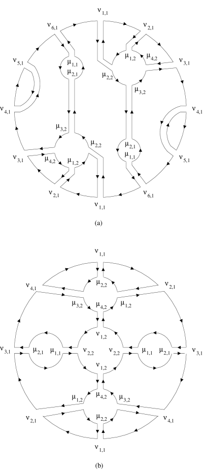
Figure 1: (a) A Feynman diagram of $G_{s}(3;1,2)$, where $s=f$ or $b$. This diagram corresponds to a vanishing term if $s=f$. (b) A Feynman diagram of $G_{s}(2,1;1,2)$. In both diagrams, the indices $\mu_{i,j}$ or $\nu_{i,j}$, where $i$ and $j$ are positive integers, are vector indices.

There is a bosonic counterpart to the fermionic model. Let $M_{1}$, $M_{2}$, …, and $M_{N_{v}}$ be complex matrices of order $N_{m}$. Out of these matrices may be constructed a bosonic matrix-vector model whose action is

$$S_{b}:=-N_{m}\sqrt{N_{v}}\sum_{\mu=1}^{N_{v}}{\rm Tr}M^{\dagger}_{\mu}M_{\mu}-\frac{N_{m}^{2}(g_{1}-1)}{2}\sum_{\mu_{1},\mu_{2}=1}^{N_{v}}\left[{\rm Tr}\left(M^{\dagger}_{\mu_{1}}M_{\mu_{2}}\right)\right]^{2}$$

$$-N_{m}\sum_{n=1}^{\infty}\frac{c_{n}}{2n}\sum_{\mu_{1},\mu_{2},\ldots,\mu_{2n}=1}^{N_{v}}{\rm Tr}\left[\left(M^{\dagger}_{\mu_{1}}M_{\mu_{2}}M^{\dagger}_{\mu_{3}}M_{\mu_{4}}\cdots M^{\dagger}_{\mu_{2n-1}}M_{\mu_{2n}}\right)^{2}\right]$$

$$-N_{m}^{2}\sum_{n=2}^{\infty}\frac{g_{n}}{2n}\sum_{\mu_{1},\mu_{2},\ldots,\mu_{2n}=1}^{N_{v}}\left[{\rm Tr}\left(M^{\dagger}_{\mu_{1}}M_{\mu_{2}}M^{\dagger}_{\mu_{3}}M_{\mu_{4}}\cdots M^{\dagger}_{\mu_{2n-1}}M_{\mu_{2n}}\right)\right]^{2}.$$

Unlike the fermionic model, those Feynman diagrams of this bosonic model in which there is no vertex representing a term whose coefficient is $c_{i}$, where $i$ is any positive integer, do not vanish. Such non-zero Feynman diagrams are also invariant under parity transformation. Let

$$Z_{b}(N_{m},N_{v}):=\int dM^{\dagger}_{1}dM_{1}dM^{\dagger}_{2}dM_{2}\cdots dM^{\dagger}_{N_{v}}dM_{N_{v}}\exp S_{b}$$ (4)

be the partition function of this model. The physical quantities we would like to evaluate are the connected Green functions

$$G_{b}(p_{1},p_{2},\ldots,p_{\tilde{n}};k_{1},k_{2},\ldots,k_{n})$$

defined as in Eq. (3) with $\bar{\Psi}$, $\Psi$ and the subscript $S_{f}$ replaced with $M^{\dagger}$, $M$, and the subscript $S_{b}$, respectively.

2.1 Schwinger–Dyson equations

We may evaluate the multiloop amplitudes of these matrix-vector models by means of Schwinger–Dyson equations. The results are intimately related to the ordinary Hermitian matrix model whose action is

$$S_{H}:=-N_{m}{\rm Tr}V(\Phi),$$

where $\Phi$ is a Hermitian matrix of order $N_{m}$ and

$$V(\Phi):=\sum_{n=1}^{\infty}\frac{g_{n}}{2n}\Phi^{2n}.$$

Let

$$\tilde{\phi}(n):=\lim_{N_{m}\rightarrow\infty}\frac{1}{N_{m}}\langle{\rm Tr}\,\Phi^{2n}\rangle_{S_{H}}$$ (5)

be the expectation value of ${\rm Tr}\,\Phi^{2n}$. Consider the trivial equations

$$\lim_{N_{m}\rightarrow\infty}\lim_{N_{v}\rightarrow\infty}\frac{1}{N_{m}^{2}\sqrt{N_{v}}Z_{f}(N_{m},N_{v})}$$

$$\cdot\sum_{i,j=1}^{N_{m}}\sum_{\alpha_{0}=1}^{N_{v}}\int d\Psi_{1}d\bar{\Psi}_{1}d\Psi_{2}d\bar{\Psi}_{2}\cdots d\Psi_{N_{v}}d\bar{\Psi}_{N_{v}}$$

$$\frac{\partial}{\partial\bar{\Psi}_{\alpha_{0}ij}}\{\sum_{\alpha_{1},\alpha_{2},\ldots,\alpha_{2n-1}=1}^{N_{v}}\left(\bar{\Psi}_{\alpha_{1}}\Psi_{\alpha_{2}}\cdots\bar{\Psi}_{\alpha_{2n-1}}\Psi_{\alpha_{0}}\bar{\Psi}_{\alpha_{1}}\Psi_{\alpha_{2}}\cdots\bar{\Psi}_{\alpha_{2n-1}}\right)_{ij}$$

$$\exp S_{f}\}=0$$

and

$$\lim_{N_{m}\rightarrow\infty}\lim_{N_{v}\rightarrow\infty}\frac{1}{N_{m}^{2}\sqrt{N_{v}}Z_{b}(N_{m},N_{v})}$$

$$\cdot\sum_{i,j=1}^{N_{m}}\sum_{\alpha_{0}=1}^{N_{v}}\int dM^{\dagger}_{1}dM_{1}dM^{\dagger}_{2}dM_{2}\cdots dM^{\dagger}_{N_{v}}dM_{N_{v}}$$

$$\frac{\partial}{\partial M^{\dagger}_{\alpha_{0}ij}}\{\sum_{\alpha_{1},\alpha_{2},\ldots,\alpha_{2n-1}=1}^{N_{v}}\left(M^{\dagger}_{\alpha_{1}}M_{\alpha_{2}}\cdots M^{\dagger}_{\alpha_{2n-1}}M_{\alpha_{0}}M^{\dagger}_{\alpha_{1}}M_{\alpha_{2}}\cdots M^{\dagger}_{\alpha_{2n-1}}\right)_{ij}$$

$$\exp S_{b}\}=0,$$

where $n$ is an arbitrary positive integer, for the fermionic and bosonic models, respectively. They yield the Schwinger–Dyson equation (see Ref. [8] for some intermediate steps),

$$2\sum_{k=0}^{n-2}\tilde{\phi}(k)G_{s}(n-1-k)+2\delta_{sb}\tilde{\phi}(n-1)$$ (6)

$$-\sum_{k=1}^{\infty}c_{k}\tilde{\phi}(n+k-1)-\sum_{k=1}^{\infty}g_{k}G_{s}(n+k-1)=0,$$

where $s=f$ or $b$, and $\delta_{sb}$ (or $\delta_{sf}$) is a Kronecker delta function. The first sum vanishes if $n=1$. Define

$$\omega_{s}(\zeta):=\sum_{n=1}^{\infty}\frac{G_{s}(n)}{\zeta^{2n+1}}$$

and

$$\chi(\zeta):=\sum_{n=1}^{\infty}\frac{\tilde{\phi}(n)}{\zeta^{2n+1}}$$

as the spectral density functions of the matrix-vector models and of the Hermitian matrix model, respectively. Then Eq. (6) leads to

$$\omega_{s}(\zeta)=\left\{-\delta_{sf}\frac{2}{\zeta^{2}}\chi(\zeta)-\sum_{k=1}^{\infty}c_{k}\zeta^{2k-2}\chi(\zeta)\right.$$

$$\left.+\sum_{k=0}^{\infty}\zeta^{2k-1}\sum_{l=0}^{\infty}\left[\tilde{\Phi}(l)c_{k+l+1}+G(l)g_{k+l+1}\right]\right\}/\left[\sum_{k=1}^{\infty}g_{k}\zeta^{2k-2}-\frac{2}{\zeta}\chi(\zeta)\right].$$

It is well known (see, e.g., Ref. [9]) that

$$\chi(\zeta)=\frac{1}{2}\left[V^{\prime}(\zeta)-M(\zeta,\beta)\sqrt{\zeta^{2}-\beta}\right],$$

where $\beta$ is determined by the integral relation

$$W(\beta):=-\frac{2}{\pi i}\int_{0}^{\sqrt{\beta}}\frac{qV^{\prime}(q)dq}{\sqrt{q^{2}-\beta}}=2,$$ (7)

and

$$M(\zeta,\beta):=\sum_{j=1}^{\infty}\zeta^{2j-2}\sum_{k=0}^{\infty}\frac{(2k)!}{4^{k}(k!)^{2}}g_{k+j}\beta^{k}.$$ (8)

Hence

$$\omega_{s}(\zeta)=\frac{1}{2}\left(\frac{2}{\zeta}\delta_{sf}+\sum_{k=1}^{\infty}c_{k}\zeta^{2k-1}\right)+\frac{P_{s}(\zeta)}{\sqrt{\zeta^{2}-\beta}},$$ (9)

where $P_{s}(\zeta)$ is a polynomial.

$P_{s}(\zeta)$ may be determined by the holomorphic properties of $\omega_{s}(\zeta)$. Multiplying both sides of Eq. (9) by $\pm i\sqrt{(\sqrt{\beta}-\zeta)(\sqrt{\beta}+\zeta)}$, we obtain

$$\pm\omega_{s}(\zeta\pm i0)i\sqrt{(\sqrt{\beta}-\zeta)(\sqrt{\beta}+\zeta)}=$$

$$\pm\frac{1}{2}\left(\frac{2}{\zeta}\delta_{sf}+\sum_{k=1}^{\infty}c_{k}\zeta^{2k-1}\right)i\sqrt{(\sqrt{\beta}-\zeta)(\sqrt{\beta}+\zeta)}+P_{s}(\zeta).$$

Thus we get a discontinuity equation

$$\left[\omega_{s}(\zeta+i0)+\omega_{s}(\zeta-i0)\right]i\sqrt{(\sqrt{\beta}-\zeta)(\sqrt{\beta}+\zeta)}=$$

$$\left(\frac{2}{\zeta}\delta_{sf}+\sum_{k=1}^{\infty}c_{k}\zeta^{2k-1}\right)i\sqrt{(\sqrt{\beta}-\zeta)(\sqrt{\beta}+\zeta)}.$$

As a result,

$$\omega_{s}(\zeta)=\frac{1}{2\pi\sqrt{\zeta^{2}-\beta}}\int_{-\sqrt{\beta}}^{\sqrt{\beta}}\frac{d\lambda\sqrt{\beta-\lambda^{2}}}{\lambda-\zeta}\left(\frac{2}{\lambda}\delta_{sf}+\sum_{k=1}^{\infty}c_{k}\lambda^{2k-1}\right)+\frac{Q_{s}(\zeta)}{\sqrt{\zeta^{2}-\beta}},$$ (10)

where $Q_{s}(\zeta)$ is a polynomial. Since $\lim_{\zeta\rightarrow\infty}\omega_{s}(\zeta)=0$, $Q_{s}(\zeta)$ is constant. Then $\lim_{\zeta\rightarrow\infty}\zeta\omega_{s}(\zeta)=1$ implies that

$$Q_{s}(\zeta)\equiv 1.$$

Evaluating the integral in Eq. (10) and comparing the result with Eq. (9) then imply

$$P_{s}(\zeta)=2\delta_{sb}-\sum_{n=1}^{\infty}c_{n}\zeta^{2n}+2\sum_{n=0}^{\infty}\zeta^{2n}\sum_{k=1}^{\infty}c_{k+n}\beta^{k}\frac{(2k-2)!}{4^{k}k!(k-1)!}.$$ (11)

We may use Eqs. (9) and (11) to expand $\omega_{s}(\zeta)$ as a power series in $1/\zeta$ and obtain all connected Green functions of the form $G_{s}(p)$.

2.2 Multiloop correlators

To obtain other connected Green functions, we apply the formula

$$G_{s}(p_{1},p_{2},\ldots,p_{\tilde{n}};k_{1},k_{2},\ldots,k_{n})$$ (12)

$$= -2p_{\tilde{n}}\frac{\partial}{\partial c_{p_{\tilde{n}}}}G_{s}(p_{1},p_{2},\ldots,p_{\tilde{n}-1};k_{1},k_{2},\ldots,k_{n})$$

$$= -2k_{n}\frac{\partial}{\partial g_{k_{n}}}G_{s}(p_{1},p_{2},\ldots,p_{\tilde{n}};k_{1},k_{2},\ldots,k_{n-1}).$$

Let

$$\omega_{s}(\zeta_{1},\zeta_{2},\ldots,\zeta_{\tilde{n}};z_{1},z_{2},\ldots,z_{n}):=$$

$$\sum_{p_{1},p_{2},\ldots,p_{\tilde{n}}=1}^{\infty}\sum_{k_{1},k_{2},\ldots,k_{n}=1}^{\infty}\frac{G_{s}(p_{1},p_{2},\ldots,p_{\tilde{n}};k_{1},k_{2},\ldots,k_{n})}{\zeta_{1}^{2p_{1}+1}\zeta_{2}^{2p_{2}+1}\cdots\zeta_{\tilde{n}}^{2p_{\tilde{n}}+1}z_{1}^{2k_{1}+1}z_{2}^{2k_{2}+1}\cdots z_{n}^{2k_{n}+1}}$$

be the multi-loop generating function of these connected Green functions. This may be paraphrased as [9]

$$\omega_{s}(\zeta;z_{1},z_{2},\ldots,z_{n})=\prod_{k=1}^{n}\left[-\sum_{j=1}^{\infty}\frac{2j}{z_{k}^{2j+1}}\left(\frac{\partial}{\partial g_{j}}\right)_{\beta}\right.$$ (13)

$$\left.+\frac{\beta}{(z_{k}^{2}-\beta)^{\frac{3}{2}}}\left(\frac{1}{W^{\prime}(\beta)}\frac{\partial}{\partial\beta}\right)_{g_{j}}\right]\left(\frac{P_{s}(\zeta)}{\sqrt{\zeta^{2}-\beta}}\right),$$

where $\left(\frac{\partial}{\partial g_{j}}\right)_{\beta}$ is the partial differentiation operator with respect to $g_{j}$ with $\beta$ held fixed, $\left(\frac{\partial}{\partial\beta}\right)_{g_{j}}$ is the partial differentiation operator with respect to $\beta$ with $g_{1}$, $g_{2}$, $g_{3}$, …, and so on held fixed, and $W(\beta)$ was defined in Eq. (7). According to Ref. [9],

$$\left[-\sum_{j=1}^{\infty}\frac{2j}{z_{k}^{2j+1}}\left(\frac{\partial}{\partial g_{j}}\right)_{\beta}+\frac{\beta}{(z_{k}^{2}-\beta)^{\frac{3}{2}}}\left(\frac{1}{W^{\prime}(\beta)}\frac{\partial}{\partial\beta}\right)_{g_{j}}\right]\left[\frac{1}{W^{\prime}(\beta)}\frac{\partial}{\partial\beta}\right]^{n}\frac{h(\beta)}{W^{\prime}(\beta)}$$

$$=\left[\frac{1}{W^{\prime}(\beta)}\frac{\partial}{\partial\beta}\right]^{n+1}\frac{h(\beta)}{W^{\prime}(\beta)}\frac{\beta}{(z_{k}^{2}-\beta)^{\frac{3}{2}}}$$

if $n$ is a non-negative integer and $h(\beta)$ is a function which depends only on $\beta$ but not $g_{1}$, $g_{2}$, $g_{3}$, …, and so on. As a result,

$$\omega_{s}(\zeta;z_{1},z_{2},\ldots,z_{n})=$$

$$\left[\frac{1}{W^{\prime}(\beta)}\frac{\partial}{\partial\beta}\right]^{n-1}\left[\frac{\delta_{sb}-\sum_{k=1}^{\infty}\frac{(2k-1)!}{4^{k}k!(k-1)!}\beta^{k}}{W^{\prime}(\beta)(\zeta^{2}-\beta)^{\frac{3}{2}}}\prod_{k=1}^{n}\frac{\beta}{(z_{k}^{2}-\beta)^{\frac{3}{2}}}\right]$$

for any positive value of $n$.

In addition, Eq. (12) implies

$$\omega_{s}(\zeta_{1},\zeta_{2})=-\frac{2\zeta_{1}\zeta_{2}}{(\zeta_{1}^{2}-\zeta_{2}^{2})^{2}}+\frac{2\zeta_{1}^{2}\zeta_{2}^{2}-\beta(\zeta_{1}^{2}+\zeta_{2}^{2})}{(\zeta_{1}^{2}-\zeta_{2}^{2})^{2}\sqrt{\zeta_{1}^{2}-\beta}\sqrt{\zeta_{2}^{2}-\beta}}.$$ (14)

Note that $\omega_{s}(\zeta_{1},\zeta_{2})$ is independent of whether the model is bosonic or fermionic and is independent of $c_{1}$, $c_{2}$, $c_{3}$, …, and so on. Thus we conclude from Eqs. (14) and (12) that

$$\omega_{s}(\zeta_{1},\zeta_{2},\ldots,\zeta_{\tilde{n}};z_{1},z_{2},\ldots,z_{n})=0$$

if $\tilde{n}\geq 3$. In other words,

$$G_{s}(p_{1},p_{2},\ldots,p_{\tilde{n}};k_{1},k_{2},\ldots,k_{n})=0$$

if $\tilde{n}\geq 3$. In terms of string worldsheet, this means that there can be only two boundaries which are invariant under parity transformation. Note also that Eq. (14) differs from the two-loop correlator of any complex matrix model by a factor of 4 only [9]. Since $\omega_{s}(\zeta_{1},\zeta_{2})$ depends on $g_{1}$, $g_{2}$, $g_{3}$, …, and so on indirectly via $\beta$ only, we could apply a formula similar to Eq. (13) to obtain other generating functions:

$$\omega_{s}(\zeta_{1},\zeta_{2};z_{1},z_{2},\ldots,z_{n})=$$ (15)

$$\left[\frac{1}{W^{\prime}(\beta)}\frac{\partial}{\partial\beta}\right]^{n-1}\left[\frac{1}{2\beta W^{\prime}(\beta)}\frac{\beta}{(\zeta_{1}^{2}-\beta)^{\frac{3}{2}}}\frac{\beta}{(\zeta_{2}^{2}-\beta)^{\frac{3}{2}}}\prod_{k=1}^{n}\frac{\beta}{(z_{k}^{2}-\beta)^{\frac{3}{2}}}\right]$$

for any positive value of $n$. These multiloop generating functions differ from those of complex matrix models merely by constant factors of $2^{n+2}$ [9]. They are basically symmetry factors of the Feynman diagrams.

2.3 Multicritical point

Following Ref. [10], we approach the $m$-th multicritical point by fine-tuning the coupling constants in such a way that there exists a real number $z_{c}$ which satisfies

$$W(\beta_{*})=W^{(k)}(\beta_{*})=0$$

for $k=1$, 2, …, and $m-1$, and

$$W^{(m)}(\beta_{*})\neq 0.$$

Then

$$W(\beta)\simeq-\gamma(\beta-\beta_{*})^{m},$$

where $\gamma$ is a complex constant, for $\beta$ close to $z_{*}$. Let

$$\zeta_{i}^{2}=\beta_{*}+a\psi_{i},\;z_{i}^{2}=\beta_{*}+a\pi_{i},\;\mbox{and}\;\beta=\beta_{*}-a\sqrt{\Lambda}$$

for any positive integer $i$, where $a$ is the cut-off length, $\Lambda$ is the renormalised bulk cosmological constant, and $\pi_{i}$ and $\psi_{i}$ are renormalised boundary cosmological constants for any value of $i$. Then

$$\frac{1}{W^{\prime}(\beta)}\frac{\partial}{\partial\beta}=-\frac{2}{m\gamma(-a)^{m}\Lambda^{\frac{m-2}{2}}}\frac{\partial}{\partial\Lambda}$$

and we may conclude that the renormalised tree-level one-loop amplitude is

$$\sqrt{a}\omega_{s}(\psi_{1})=\frac{2\delta_{sb}+\sum_{n=1}^{\infty}\beta_{*}^{n}c_{n}\left[2\sum_{k=1}^{n}\frac{(2k-2)!}{4^{k}k!(k-1)!}-1\right]}{(\psi_{1}+\sqrt{\Lambda})^{\frac{1}{2}}},$$

and the renormalised tree-level multi-loop amplitudes are

$$a^{(m+\frac{3}{2})n+\frac{1}{2}}\omega_{s}(\psi_{1};\pi_{1},\pi_{2},\ldots,\pi_{n};\Lambda)=$$

$$\frac{(-1)^{mn+n+1}2^{n-2}\beta_{*}^{n}\left[1-\sum_{k=1}^{\infty}\frac{(2k-1)!}{4^{k}k!(k-1)!}\beta_{*}^{k}\right]}{m^{n}\gamma^{n}}$$

$$\cdot\left(\frac{1}{\Lambda^{\frac{m}{2}-\delta_{sb}}}\frac{\partial}{\partial\Lambda}\right)^{n-1}\left[\frac{1}{\Lambda^{\frac{m-1}{2}}}\frac{1}{(\psi_{1}+\sqrt{\Lambda})^{\frac{3}{2}}}\prod_{k=1}^{n}\frac{1}{(\pi_{i}+\sqrt{\Lambda})^{\frac{3}{2}}}\right]$$

for $n\geq 1$,

$$a^{2}\omega_{s}(\psi_{1},\psi_{2})=-\frac{2\beta_{*}}{(\psi_{1}-\psi_{2})^{2}}+\frac{(\psi_{1}+\psi_{2}+2\sqrt{\Lambda})\beta_{*}}{(\psi_{1}-\psi_{2})^{2}(\psi_{1}+\sqrt{\Lambda})^{\frac{1}{2}}(\psi_{2}+\sqrt{\Lambda})^{\frac{1}{2}}}$$

and

$$a^{(m+\frac{3}{2})n+2}\omega_{s}(\psi_{1},\psi_{2};\pi_{1},\pi_{2},\ldots,\pi_{n};\Lambda)=$$

$$\frac{(-1)^{mn+n}\beta_{*}^{n+1}}{4m^{n}\gamma^{n}}\left(\frac{1}{\Lambda^{\frac{m}{2}-1}}\frac{\partial}{\partial\Lambda}\right)^{n}$$

$$\cdot\left[\frac{1}{\Lambda^{\frac{m-1}{2}}(\psi_{1}+\sqrt{\Lambda})^{\frac{3}{2}}(\psi_{2}+\sqrt{\Lambda})^{\frac{3}{2}}}\prod_{k=1}^{n}\frac{1}{(\pi_{i}+\sqrt{\Lambda})^{\frac{3}{2}}}\right]$$

for $n\geq 1$.

3 Multicritical models of ${\mathbb{R}}^{2}/{\mathbb{Z}}_{2}$

Let us turn our attention to multicritical models of the quantum orbifold ${\mathbb{R}}^{2}/{\mathbb{Z}}_{2}$. The action of the bosonic version is

$$\tilde{S}_{b}:=-N_{m}\sqrt{N_{v}}\sum_{\mu=1}^{N_{v}}{\rm Tr}M^{\dagger}_{\mu}M_{\mu}$$

$$-\frac{N_{m}^{2}(g_{1}-1)}{2}\sum_{\mu_{1},\mu_{2}=1}^{N_{v}}{\rm Tr}\left(M^{\dagger}_{\mu_{1}}M_{\mu_{2}}\right){\rm Tr}\left(M_{\mu_{2}}M^{\dagger}_{\mu_{1}}\right)$$

$$-N_{m}\sum_{n=1}^{\infty}c_{n}\sum_{\mu_{1},\mu_{2},\ldots,\mu_{2n}=1}^{N_{v}}{\rm Tr}\left(M^{\dagger}_{\mu_{1}}M_{\mu_{2}}M^{\dagger}_{\mu_{3}}M_{\mu_{4}}\cdots M^{\dagger}_{\mu_{2n-1}}M_{\mu_{2n}}\right.$$

$$\left.\cdot M_{\mu_{2n}}M^{\dagger}_{\mu_{2n-1}}M_{\mu_{2n-2}}M^{\dagger}_{\mu_{2n-3}}\cdots M_{\mu_{2}}M^{\dagger}_{\mu_{1}}\right)$$

$$-N_{m}^{2}\sum_{n=2}^{\infty}\frac{g_{n}}{2n}\sum_{\mu_{1},\mu_{2},\ldots,\mu_{2n}=1}^{N_{v}}{\rm Tr}\left(M^{\dagger}_{\mu_{1}}M_{\mu_{2}}M^{\dagger}_{\mu_{3}}M_{\mu_{4}}\cdots M^{\dagger}_{\mu_{2n-1}}M_{\mu_{2n}}\right)$$

$$\cdot{\rm Tr}\left(M_{\mu_{2n}}M^{\dagger}_{\mu_{2n-1}}M_{\mu_{2n-2}}M^{\dagger}_{\mu_{2n-3}}\cdots M_{\mu_{2}}M^{\dagger}_{\mu_{1}}\right),$$

whereas the action of the fermionic version is [8]

$$\tilde{S}_{f}:=-N_{m}\sqrt{N_{v}}\sum_{\mu=1}^{N_{v}}{\rm Tr}\bar{\Psi}_{\mu}\Psi_{\mu}$$

$$-\frac{N_{m}^{2}(g_{1}-1)}{2}\sum_{\mu_{1},\mu_{2}=1}^{N_{v}}{\rm Tr}\left(\bar{\Psi}_{\mu_{1}}\Psi_{\mu_{2}}\right){\rm Tr}\left(\Psi_{\mu_{2}}\bar{\Psi}_{\mu_{1}}\right)$$

$$-N_{m}\sum_{n=1}^{\infty}c_{n}\sum_{\mu_{1},\mu_{2},\ldots,\mu_{2n}=1}^{N_{v}}{\rm Tr}\left(\bar{\Psi}_{\mu_{1}}\Psi_{\mu_{2}}\bar{\Psi}_{\mu_{3}}\Psi_{\mu_{4}}\cdots\bar{\Psi}_{\mu_{2n-1}}\Psi_{\mu_{2n}}\right.$$

$$\left.\cdot\Psi_{\mu_{2n}}\bar{\Psi}_{\mu_{2n-1}}\Psi_{\mu_{2n-2}}\bar{\Psi}_{\mu_{2n-3}}\cdots\Psi_{\mu_{2}}\bar{\Psi}_{\mu_{1}}\right)$$

$$-N_{m}^{2}\sum_{n=2}^{\infty}\frac{g_{n}}{2n}\sum_{\mu_{1},\mu_{2},\ldots,\mu_{2n}=1}^{N_{v}}{\rm Tr}\left(\bar{\Psi}_{\mu_{1}}\Psi_{\mu_{2}}\bar{\Psi}_{\mu_{3}}\Psi_{\mu_{4}}\cdots\bar{\Psi}_{\mu_{2n-1}}\Psi_{\mu_{2n}}\right)$$

$$\cdot{\rm Tr}\left(\Psi_{\mu_{2n}}\bar{\Psi}_{\mu_{2n-1}}\Psi_{\mu_{2n-2}}\bar{\Psi}_{\mu_{2n-3}}\cdots\Psi_{\mu_{2}}\bar{\Psi}_{\mu_{1}}\right).$$

Note that the second terms in these actions may be represented by a pair of Feynman propagators. The partition functions of the bosonic and fermionic models are defined as in Eqs. (4) and (2), respectively, with $Z$ replaced with $\tilde{Z}$ and $S$ with $\tilde{S}$. For the bosonic model, the connected Green functions which we would like to study take the form

$$\tilde{G}_{b}(p_{1},p_{2},\ldots,p_{\tilde{n}};k_{1},k_{2},\ldots,k_{n}):=\lim_{N_{m}\rightarrow\infty}\lim_{N_{v}\rightarrow\infty}N_{m}^{\tilde{n}+2n-2}$$ (16)

$$\sum_{\nu_{1,1},\nu_{2,1},\ldots,\nu_{2p_{1},1}=1}^{N_{v}}\sum_{\nu_{1,2},\nu_{2,2},\ldots,\nu_{2p_{2},2}=1}^{N_{v}}\cdots\sum_{\nu_{1,\tilde{n}},\nu_{2,\tilde{n}},\ldots,\nu_{2p_{\tilde{n}},\tilde{n}}=1}^{N_{v}}$$

$$\sum_{\mu_{1,1},\mu_{2,1},\ldots,\mu_{2k_{1},1}=1}^{N_{v}}\sum_{\mu_{1,2},\mu_{2,2},\ldots,\mu_{2k_{2},2}=1}^{N_{v}}\cdots\sum_{\mu_{1,n},\mu_{2,n},\ldots,\mu_{2k_{n},n}=1}^{N_{v}}$$

$$\left\langle\prod_{j=1}^{\tilde{n}}{\rm Tr}\left(M^{\dagger}_{\nu_{1,j}}M_{\nu_{2,j}}M^{\dagger}_{\nu_{3,j}}M_{\nu_{4,j}}\cdots M^{\dagger}_{\nu_{2p_{j}-1,j}}M_{\nu_{2p_{j},j}}\right.\right.$$

$$\left.\cdot M_{\nu_{2p_{j},j}}M^{\dagger}_{\nu_{2p_{j}-1,j}}M_{\nu_{2p_{j}-2,j}}M^{\dagger}_{\nu_{2p_{j}-3,j}}\cdots M_{\nu_{2,j}}M^{\dagger}_{\nu_{1,j}}\right)$$

$$\cdot\prod_{i=1}^{n}{\rm Tr}\left(M^{\dagger}_{\mu_{1,i}}M_{\mu_{2,i}}M^{\dagger}_{\mu_{3,i}}M_{\mu_{4,i}}\cdots M^{\dagger}_{\mu_{2k_{i}-1,i}}M_{\mu_{2k_{i},i}}\right)$$

$$\cdot\left.{\rm Tr}\left(M_{\mu_{2k_{i},i}}M^{\dagger}_{\mu_{2k_{i}-1,i}}M_{\mu_{2k_{i}-2,i}}M^{\dagger}_{\mu_{2k_{i}-3,i}}\cdots M_{\mu_{2,i}}M^{\dagger}_{\mu_{1,i}}\right)\right\rangle_{{\rm conn},\tilde{S}_{b}},$$

where $n$ is any non-negative integer, $\tilde{n}$ is any positive integer, and $p_{1}$, $p_{2}$, …, $p_{\tilde{n}}$, $k_{1}$, $k_{2}$, …, and $k_{n}$ are any positive integers; for the fermionic model, the connected Green functions which we would like to study also take the form in Eq. (16) with $M$, $M^{\dagger}$, and $\tilde{S}_{b}$ replaced with $\Psi$, $\bar{\Psi}$, and $\tilde{S}_{f}$, respectively. A Feynman diagram representing a term in a connected Green function is depicted in Fig. 2.

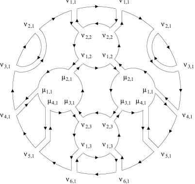
Figure 2: A Feynman diagram of $\tilde{S}_{b}(3,1,1;2)$.

3.1 Schwinger–Dyson equations

To evaluate the connected Green functions at the double large-$N$ limit, let us start with the trivial equation

$$\lim_{N_{m}\rightarrow\infty}\lim_{N_{v}\rightarrow\infty}\frac{1}{N_{m}^{2}\sqrt{N_{v}}Z^{\prime}_{b}(N_{m},N_{v})}$$ (17)

$$\cdot\sum_{i,j=1}^{N_{m}}\sum_{\alpha_{0}=1}^{N_{v}}\int dM^{\dagger}_{1}dM_{1}dM^{\dagger}_{2}dM_{2}\cdots dM^{\dagger}_{N_{v}}dM_{N_{v}}$$

$$\frac{\partial}{\partial M^{\dagger}_{\alpha_{0}ij}}\{\sum_{\alpha_{1},\alpha_{2},\ldots,\alpha_{2n-1}=1}^{N_{v}}\left(M^{\dagger}_{\alpha_{2n-1}}M_{\alpha_{2n-2}}\cdots M^{\dagger}_{\alpha_{1}}\right.$$

$$\cdot\left.M^{\dagger}_{\alpha_{1}}M_{\alpha_{2}}\cdots M^{\dagger}_{\alpha_{2n-1}}M_{\alpha_{0}}\right)_{ij}\exp\tilde{S}_{b}\}=0$$

for the bosonic model or

$$\lim_{N_{m}\rightarrow\infty}\lim_{N_{v}\rightarrow\infty}\frac{1}{N_{m}^{2}\sqrt{N_{v}}Z^{\prime}_{f}(N_{m},N_{v})}\sum_{i,j=1}^{N_{m}}\sum_{\alpha_{0}=1}^{N_{v}}\int d\Psi_{1}d\bar{\Psi}_{1}d\Psi_{2}d\bar{\Psi}_{2}\cdots d\Psi_{N_{v}}d\bar{\Psi}_{N_{v}}$$ (18)

$$\frac{\partial}{\partial\bar{\Psi}_{\alpha_{0}ij}}\{\sum_{\alpha_{1},\alpha_{2},\ldots,\alpha_{2n-1}=1}^{N_{v}}\left(\bar{\Psi}_{\alpha_{2n-1}}\Psi_{\alpha_{2n-2}}\cdots\bar{\Psi}_{\alpha_{1}}\bar{\Psi}_{\alpha_{1}}\Psi_{\alpha_{2}}\cdots\bar{\Psi}_{\alpha_{2n-1}}\Psi_{\alpha_{0}}\right)_{ij}$$

$$\exp\tilde{S}_{f}\}=0$$

for the fermionic model. Both Eqs. (17) and (18) lead to the Schwinger–Dyson equation

$$\sum_{k=1}^{n}\tilde{\phi}(n-k)\tilde{G}(k-1)$$ (19)

$$-\sum_{k=1}^{\infty}c_{k}\sum_{l=1}^{k}\tilde{G}(l-1)\tilde{G}(n+k-l)-\sum_{k=1}^{\infty}g_{k}\tilde{G}(n+k-1)=0,$$

where $n$ is any positiver integer, $\tilde{G}(n)$ stands for $\tilde{G}_{b}(n)$ or $\tilde{G}_{f}(n)$, and $\tilde{\phi}(n)$ was defined in Eq. (5). Hence the connected Green functions of the bosonic model at the double large-$N$ limit are identical to those of the fermionic model.

Let

$$\tilde{\omega}(\zeta):=\sum_{n=1}^{\infty}\frac{\tilde{G}(n)}{\zeta^{2n+1}}$$

be the spectral function of these matrix-vector models. It then follows from Eq. (19) and the well-known expression for the spectral function $\chi(\zeta)$ of the ordinary Hermitian matrix model that

$$\tilde{\omega}(\zeta) = \frac{2Q_{1}(\zeta)}{Q_{2}(\zeta)+M(\zeta,\beta)\sqrt{\zeta^{2}-\beta}},$$ (20)

$$= \frac{2Q_{1}(\zeta)\left[Q_{2}(\zeta)-M(\zeta,\beta)\sqrt{\zeta^{2}-\beta}\right]}{Q_{2}^{2}(\zeta)-M^{2}(\zeta,\beta)(\zeta^{2}-\beta)}$$ (21)

where $\beta$ and $M(\zeta,\beta)$ were defined in Eqs. (7) and (8),

$$Q_{1}(\zeta):=\sum_{k=1}^{\infty}\zeta^{2k-2}\sum_{l=0}^{\infty}g_{k+l}\tilde{G}(l)+\sum_{k=0}^{\infty}\zeta^{2k}\sum_{l=0}^{\infty}\tilde{G}(l)\sum_{m=0}^{\infty}\tilde{G}(m)c_{k+l+m+1},$$ (22)

and

$$Q_{2}(\zeta):=\sum_{k=1}^{\infty}g_{k}\zeta^{2k-1}+2\sum_{k=0}^{\infty}\zeta^{2k+1}\sum_{l=0}^{\infty}\tilde{G}(l)c_{k+l+1}.$$ (23)

As usual, we assert that the values of the connected Green functions in Eqs. (22) and (23) are determined by the requirement that $\tilde{\omega}$ be holomorphic on the whole complex plane except the branch cut $-\sqrt{\beta}\leq\Re(\zeta)\leq\sqrt{\beta}$ and $\Im(\zeta)=0$.

3.2 Some multicritical points

A convenient choice of the $m$-th multicritical point is to select a non-zero value of $g_{m}$, adjust the values of $g_{1}$, $g_{2}$, …, and $g_{m-1}$ such that

$$M(\zeta)=g_{m}(\zeta^{2}-\beta)^{m-1},$$

and adjust the values of $c_{1}$, $c_{2}$, …, and $c_{m}$ such that

$$Q_{2}(\zeta)=g_{m}\zeta(\zeta^{2}-\beta)^{m-1}.$$ (24)

Moreover, $g_{n}=c_{n}=0$ if $n>m\geq 2$. It then follows from Eq. (20) that

$$\tilde{\omega}(\zeta)=\frac{2Q_{1}(\zeta)(\zeta-\sqrt{\zeta^{2}-\beta})}{g_{m}\beta(\zeta^{2}-\beta)^{m-1}}.$$ (25)

The holomorphic property of $\tilde{\omega}(\zeta)$ then dictates that the zeros of $Q_{1}(\zeta)$ coincide with the zeros of the denominator on the right side of Eq. (25). As a result, at the $m$-th multicritical point,

$$Q_{1}(\zeta)=A(\zeta^{2}-\beta)^{m-1};$$ (26)

the constant $A$ may be determined by the condition that

$$\lim_{\zeta\rightarrow\infty}\zeta\tilde{\omega}(\zeta)=1.$$

This yields $A=g_{m}$. As a result,

$$\tilde{\omega}(\zeta)=\frac{2}{\beta}\left(\zeta-\sqrt{\zeta^{2}-\beta}\right)$$

at the $m$-th multicritical point.

A convenient way to approach the $m$-th multicritical point is to keep the ratios $g_{i}:g_{j}$, $g_{i}:c_{j}$, and $c_{i}:c_{j}$, where $i$ and $j$ are positive integers less than or equal to $m$, fixed. Then in Eq. (20), only $\zeta$ and $\beta$ deviates from their critical values $\sqrt{\beta_{*}}$ and $\beta_{*}$, respectively, whereas $g_{k}$, $c_{k}$, and $\tilde{G}(k)$, where $k$ is any positive integer not larger than $m$, are fixed. Let

$$\zeta^{2}=\beta_{*}+a\pi\;\mbox{and}\;\beta=\beta_{*}-a\sqrt{\Lambda},$$

where $a$ is the cut-off length, and $\pi$ and $\Lambda$ are the boundary and bulk cosmological constants, respectively. Then $Q_{1}(\zeta)$, $Q_{2}(\zeta)$, and $M(\zeta)$ are of order $a^{m-1}$, whereas $\sqrt{\zeta^{2}-\beta}$ is of order $\sqrt{a}$. Recall that $M(\zeta)\sqrt{\zeta^{2}-\beta}$ is, up to a proportionality constant, also the singular part of the spectral function of ordinary Hermitian matrix models. Hence we conclude from Eqs. (21), (24), and (26) that we may multiply $\tilde{\omega}$ by $\sqrt{a}$ to obtain the renormalised tree-level one-loop amplitude which, up to a constant factor, is

$$\frac{1}{\pi^{m-1}}\left(\begin{array}[]{c}\mbox{renormalised 1-loop amplitude of}\\ \mbox{an ordinary Hermitian matrix model}\\ \mbox{at the $m$-th multicritical point}\end{array}\right).$$

4 Conclusion and Outlook

We may study quantum orbifold geometry by means of bosonic or fermionic matrix-vector models. As for the quantum orbifold ${\mathbb{R}}^{2}/{\mathbb{Z}}_{2}\times{\mathbb{Z}}_{2}$, the bosonic model differs from the fermionic model in the sense that Feynman diagrams with no $c_{i}$-vertices, where $i$ is any positive integer, contribute to the Green functions of the bosonic model only; they have no contribution to those of the fermionic model. If in an orbifolded worldsheet there is only one boundary which is invariant under parity transformation, then its multiloop amplitude is significantly different from that of an ordinary worldsheet. Nonetheless, if there are two boundaries which are invariant under parity transformation, then its multiloop amplitude is the same as that of an ordinary worldsheet up to a symmetry factor.

As for the quantum orbifold ${\mathbb{R}}^{2}/{\mathbb{Z}}_{2}$, the bosonic and fermionic models are equivalent to each other at the double large-$N$ limit. The renormalised tree-level one-loop amplitude at an $m$-th multicritical point differs from that of an ordinary Hermitian matrix model by a factor inversely proportional to $\pi^{m-1}$. Nevertheless, it may be possible to identify other $m$-th multicritical points at which the quantum orbifold may behave differently. It would also be of interest to obtain more explicity expressions for higher loop amplitudes of this quantum orbifold. Furthermore, exploring the double-scaling limit of these matrix-vector models would give us valuable information on the non-perturbative behavior of unoriented string theory.

Acknowledgment

I thank A. Nica and R. Szabo for discussions. This work is partially supported by the Pure Mathematics Department at the University of Waterloo.

References

- [1] P. Di Francesco, P. Ginsparg, and J. Zinn-Justin, 2-D gravity and random matrices, Phys. Rept. 254 (1995) 1—133 [hep-th/9306153].
- [2] J. McGreevy and H. Verlinde, Strings from tachyons: the = 1 matrix reloaded [hep-th/0304224].
- [3] M. R. Douglas, I. R. Klebanov, D. Kutasov, J. Maldacena, E. Martinec, and N. Seiberg, A new hat for the = 1 matrix model [hep-th/0307195].
- [4] G. Pradisi and A. Sagnotti, Open string orbifolds, Phys. Lett. B 216 (1989) 59—67.
- [5] P. Hořava, Strings on world-sheet orbifolds, Nucl. Phys. B 327 (1989) 461—484.
- [6] J. H. Schwarz, in Strings, branes and gravity: lecture notes TASI 99 Boulder, Colorado, USA 31 May — 25 June 1999, ed. J. A. Harvey et al. (World Scientific, 1999) pp.809—846 [hep-th/9908144].
- [7] P. Biane, F. Goodman, and A. Nica, Non-crossing cumulants of type B, math.OA/0206167.
- [8] C.-W. H. Lee, Noncommutative probability, matrix models, and quantum orbifold geometry, JHEP 06 (2003) 044 [hep-th/0303086].
- [9] J. Ambjørn, J. Jurkiewicz, and Yu. M. Makeenko, Multiloop correlators for two-dimensional quantum gravity, Phys. Lett. B 251 (1990) 517—524
- [10] V. A. Kazakov, The appearance of matter fields from quantum fluctuations of 2D-gravity, Mod. Phys. Lett. A (1989) 2125—2139.