Abstract: In these lectures, we review the physics of time–dependent orbifolds of string theory, with particular attention to orbifolds of three–dimensional Minkowski space. We discuss the propagation of free particles in the orbifold geometries, together with their interactions. We address the issue of stability of these string vacua and the difficulties in defining a consistent perturbation theory, pointing to possible solutions. In particular, it is shown that resumming part of the perturbative expansion gives finite amplitudes. Finally we discuss the duality of some orbifold models with the physics of orientifold planes, and we describe cosmological models based on the dynamics of these orientifolds.

1 Introduction

A fundamental problem of theoretical physics is concerned with the nature of the initial cosmological singularity. General relativity, which describes the universe at large scales [1], predicts that, under generic assumptions, the universe went through a phase of high curvature, where quantum gravity should have been important. Hence, the reasons behind the present evolution of the universe can only be answered by understanding the Planck era. At the present stage of our knowledge, string theory is the most developed [2, 3], even though still far from complete, description of gravitational quantum phenomena, and therefore should provide the right tools to address such fundamental question.

To investigate quantum gravity effects at the cosmological singularity, there has been, over the past two years, a considerable activity in the development of time–dependent string orbifolds. In this review we shall give an introduction to the subject. We shall not give a detailed analysis of all the time–dependent orbifolds in the literature, since we will mostly concentrate on the orbifolds of three–dimensional Minkowski space, but we will provide a guide through the basic techniques in the subject. The subject is very young, far from being clearly understood, so that the problems we address are still quite basic, starting from a consistent definition of time–dependent string vacua. Recent developments in the field have shown that perturbation theory breaks down in many time–dependent orbifolds, leading to the belief that a strong coupling problem arises, similar to the case of black hole curvature singularities. We shall give some evidence that these divergences can actually be resolved, and therefore that time–dependent string orbifolds are, in fact, a good laboratory for studying the physics of the cosmological singularity.

Let us review a simplified version of the singularity theorems [1]. Consider a four–dimensional FRW universe with metric

$$ds^{2}=-dt^{2}+a^{2}(t)\,ds^{2}\left(\mathcal{M}\right)\ ,$$

where $\mathcal{M}$ is a maximally symmetric space. From Einstein equations one immediately concludes that

$$\dot{H}=-4\pi G\,\left(\rho+p\right)\ +\frac{k}{a^{2}}\ ,$$

where $H=\dot{a}/a$ is the Hubble parameter and where $\rho$ and $p$ are the matter energy density and pressure, respectively. If $k=0,-1$ and matter satisfies the null energy condition $\rho+p\geq 0$, then the universe cannot reverse from a contracting phase ($H<0$) to an expanding phase ($H>0$). Moreover, from Einstein equations it also follows that

$$\frac{\ddot{a}}{a}=-\frac{4\pi G}{3}\,\left(\rho+3p\right)\,.$$

Thus, if the stronger strong energy condition $\rho+3p\geq 0$ holds, then for any curvature $k$, as we go back in time, we expect an initial singularity [1]. In this case, one immediately faces the horizon problem, because today’s observable universe consisted, at the Planck era, of $(10^{30})^{3}$ causally disconnected regions. If, on the other hand, only the null energy condition holds, then we can have a non–singular behavior in the past, or just a coordinate singularity, usually signalling the presence of cosmological horizons. Note that a scalar field $\phi$ with potential energy $V(\phi)$ has energy density and pressure given by

$$\rho=\frac{1}{16\pi G}\left(\frac{1}{2}\,\dot{\phi}^{\,2}+V(\phi)\right)\ ,\ \ \ \ \ \ \ \ \ \ \ p=\frac{1}{16\pi G}\left(\frac{1}{2}\,\dot{\phi}^{\,2}-V(\phi)\right)\ ,$$

and therefore generically satisfies the null energy condition, but not the strong one. This fact is the basis of the solution of the horizon problem based on inflation [4].

Currently there are two conventional ways of thinking about the cosmological singularity problem. One possibility is to describe the singularity by a quantum gravity initial state from which the universe inflated [5]. Alternatively, the universe went through a bounce where quantum gravity was relevant. Here various scenarios have been considered in the literature. In the Veneziano pre big–bang model [6] and in the ekpyrotic model [7] initial conditions must be set in the far past before the bang in order to solve the homogeneity and flatness problems. This problem of initial conditions can be solved, within the ekpyrotic setup, with the cyclic model [8], where the observed homogeneity, flatness and density perturbations are dynamically generated by periods of dark energy domination before the bangs. Moreover, the big–bang singularity of the ekpyrotic and cyclic models are given by a specific time–dependent orbifold of M–theory [9]. The problem of defining transition amplitudes across the singularity has received considerable attention in the literature [10], however it is far from being settled in quantum gravity. Therefore, this question ought to be addressed in string theory and, in particular, time–dependent string orbifolds are useful models, where one has computational power to investigate the high curvature cosmological phase. Additionally, a new possibility for the universe global structure, where the conventional curvature singularity is replaced by a past cosmological horizon, will be derived from a string theory orbifold construction.

This review is organized as follows. In section 2 we describe generalities of time–dependent orbifolds [11] such as their classification, geometry, single particle wave functions, free particle propagation and linear backreaction. We shall work out in detail the time–dependent orbifolds of three–dimensional flat space. Each example is reasonably self–contained, so that the reader has at his/her disposal an independent review of the basic facts about each orbifold.

Section 3 will be devoted to the important topic of particle interactions. We shall start by reviewing the non–linear response of the gravitational field when a particle is placed in the orbifold geometry. This includes the argument for formation of large black holes put forward by Horowitz and Polchinski [12], and a particular exact solution of the problem that uses the powerful techniques of two–dimensional dilaton gravity [13, 14]. Then we consider tree level particle interactions, deriving the divergences that appear in the four–point amplitude at specific kinematical regimes, as found by Liu, Moore and Seiberg [15, 16, 17]. It is shown that these divergences can be cured by using the eikonal approximation which resums generalized ladder graphs [18]. Moreover, we shall see, with a specific example, that the Horowitz–Polchinski non–linear gravitational instability and the breakdown of perturbation theory are unrelated, contrary to claims in the literature. Finally, we describe the present status of the one loop string amplitude computations [19, 20, 15], and we analyze the wave functions of on–shell winding states [21].

In section 4 we review a new cosmological scenario in string theory, which we call orientifold cosmology, where the presence of negative tension branes generates a cosmological bounce [22]. In this scenario, the standard cosmological singularity is replaced be a past cosmological horizon [23, 24, 19]. Behind the horizon there is a time–like naked singularity, interpreted as a negative tension brane [22, 25]. We shall start by establishing a duality between a specific M–theory orbifold and a type IIA orientifold $8$–plane [14, 18]. This duality is relevant for describing the near–singularity limit of a two–dimensional toy cosmology associated to the bounce of an $O8/\overline{O}8$ pair. Using a flux compactification in supergravity, this construction is extended to the case of a four–dimensional cosmology, which is shown to exhibit cyclic periods of acceleration during the cosmological expansion [26].

We conclude in section five. For an extensive list of references on time–dependent orbifolds of flat and curved spaces, together with related work, see references [27]–[59].

2 Time–dependent orbifolds

Given a conformal field theory (CFT) which is invariant under the action of a discrete group $\Gamma$, there is a well known procedure to construct a new CFT [60]: (1) Add a twisted sector to the theory satisfying

$$\phi(\sigma^{1}+2\pi)=h\,\phi(\sigma^{1})\ ,\ \ \ \ \ \ \ \ \ \ \ \ \ \ h\in\Gamma\ ,$$

where $\phi$ is a conformal field and $\sigma^{1}$ the space–like worldsheet coordinate; (2) Restrict the spectrum to $\Gamma$–invariant states. The new theory is called an orbifold of the old CFT. In string theory, the bosonic conformal fields are the target space fields $X^{a}(\sigma)$. Then, when the group $\Gamma$ is a discrete subgroup of the target space isometries, the orbifold theory describes strings propagating on the quotient space.

The simplest example of an orbifold is toroidal compactification. One breaks the Lorentz group of $D$–dimensional Minkowski space to $SO(D-2,1)\times U(1)$, by identifying points under a discrete translation by $2\pi R$ along some direction. Then, winding strings are added, and the spectrum is restricted by quantizing the momentum along the compact direction. Another example, which is a close analogue of the orbifolds we shall be interested in, is the $\mathbb{Z}_{N}$ orbifold, where the discrete subgroup $\Gamma\sim\mathbb{Z}_{N}$ is generated by a rotation $r$ on a plane by an angle $2\pi/N$. The group $\Gamma$ consists of the elements of the form $r^{n}$, with $n\in\{0,\dots,N-1\}$. Moreover, the quotient space is a cone, which has a delta function curvature singularity. It turns out that string theory is well defined on this singular space. This is an intrinsically stringy phenomenon, since one is forced to add twisted states, which wind around the tip of the cone, to have a well defined and finite perturbation theory (for example, a modular invariant partition function) [60].

The fact that string theory can resolve space–time singularities (the conifold being another example [61, 62]), led many authors to the investigation of string orbifolds where the group action on the target space generates time–dependent quotient spaces. In particular, one would hope that possible singularities could be harmless, just like in the previous example. Unfortunately, things are more complicated, but nevertheless one still has cosmological space–times where the string coupling and the curvature are under control. Moreover, we shall see that the situation for some orbifold cosmological singularities is clearly better than the still unsolved black hole singularities.

2.1 Orbifold classification and generalities

Consider a Killing vector field $\kappa$ on a manifold $\mathcal{M}$ with isometry group $G$. Points along the orbits of $\kappa$ can be identified according to

$$P\sim e^{n\kappa}P\ ,\ \ \ \ \ \ \ \ \ \ \ \ \ \ n\in\mathbb{Z}\ ,$$

where $e^{\kappa}$ generates a discrete subgroup $\Gamma\subset G$, isomorphic to $\mathbb{Z}$ or $\mathbb{Z}_{N}$. Killing vectors related by conjugation by $G$

$$\kappa\rightarrow h^{-1}\kappa\,h\ ,\ \ \ \ \ \ \ \ \ \ \ \ \ \ h\in G\ ,$$

define the same orbifold. Here we shall analyze in detail the simplest cases of time–dependent orbifolds, in particular, we shall consider the covering space $\mathcal{M}$ to be the flat three–dimensional Minkowski space $\mathbb{M}^{3}$. The model can then be embedded in a critical string theory adding extra spectator directions.

To classify the orbifolds of $\mathbb{M}^{3}$ of the type described above, we therefore simply have to analyze the Killing vectors of $\mathbb{M}^{3}$, up to conjugation by $ISO\left(2,1\right)$. Let us start by introducing Minkowski coordinates $X^{0}$, $X^{1}$, $X^{2}$ and light–cone coordinates

$$X^{\pm}=\frac{1}{\sqrt{2}}\left(X^{0}\pm X^{1}\right)\,.$$

A general Killing vector $\kappa$ is of the form

$$\kappa=2\pi i\left(\alpha^{a}P_{a}+\beta^{ab}J_{ab}\right)\,,$$

where

$$iJ_{ab} = X_{a}\partial_{b}-X_{b}\partial_{a}\,,$$

$$iP_{a} = \partial_{a}\,,$$

are the usual generators of the Poincaré algebra. In three dimensions the situation is quite simple, since we can define the dual form to $\beta^{ab}$ by

$$\beta^{ab}=\epsilon^{abc}\beta_{c}\,.$$ (1)

If we consider conjugating $\kappa$ with an element $h\in SO\left(2,1\right)\subset ISO\left(2,1\right)$, then the vectors $\alpha^{a}$ and $\beta_{a}$ transform by the corresponding (hyper)rotation. If, on the other hand, $h$ is an infinitesimal translation, then

$$\alpha^{a} \rightarrow \alpha^{a}+\beta^{ab}\omega_{b}\,\,,$$ (2)

$$\beta^{ab} \rightarrow \beta^{ab}\,,$$

with $\omega_{a}$ infinitesimal. Therefore, using (1), it is simple to see that the two quantities

$$\alpha^{a}\beta_{a}\,,\ \ \ \ \ \ \ \ \ \ \ \ \ \beta^{a}\beta_{a}$$

are invariant under conjugation. We shall assume that $\beta_{a}\neq 0$ (otherwise we have a pure translation orbifold). Then, depending on the sign of $\beta^{2}$, we have an elliptic ($\beta^{2}<0$), hyperbolic ($\beta^{2}>0$) or parabolic ($\beta^{2}=0$) orbifold, and the two invariants just described characterize completely the orbifold.

Let us start with the hyperbolic orbifolds, where we can choose, after a Lorentz transformation, $\beta_{2}=\Delta$, $\beta_{\pm}=0$. Using (2) we can eliminate $\alpha^{\pm}$, and we are left with $\alpha^{2}=R$. Therefore we have arrived at the general hyperbolic orbifold, parametrized by a two–parameter family of inequivalent conjugacy classes, given by

$$\kappa=2\pi i\,\left(\Delta\,J_{+-}+R\,P_{2}\right)\,,$$ (3)

and generated by a boost along one direction, say the $X^{1}$–direction, and a translation along the transverse $X^{2}$–direction [19]. In this review, we shall call this orbifold the shifted–boost orbifold, whenever $R\neq 0$. The particular case with $R=0$ gives the boost orbifold first studied in [9], which is relevant for the ekpyrotic universe.

Secondly, we can consider the parabolic orbifolds, with $\beta_{-}=\Delta$, and $\alpha^{-}=R$. In this case, the inequivalent conjugacy classes are given uniquely by the invariant $\alpha\cdot\beta=\Delta R$, and are defined by the Killing vector

$$\kappa=2\pi i\,\left(\Delta\,J_{+2}+R\,P_{-}\right)\,.$$ (4)

We will denote the case $R\neq 0$ the $O$–plane orbifold [18]. The unconventional nomenclature will be justified in section 4. Setting $R=0$ one obtains the null–boost orbifold considered in [28, 15]. Adding a translation along a fourth spatial direction to the null boost generator, therefore considering an orbifold of $\mathbb{M}^{4}$, one obtains the so–called null–brane orbifold , which has been studied in the literature in [63, 16, 32]. We shall comment on this orbifold throughout the review, but will not give the details, which are a simple generalization of the null–boost orbifold.

Table 1: Time–dependent orbifolds of $\hbox{\mybb M}^{3}$.

Orbifold	Generator
Shifted–boost	$2\pi i\left(\Delta\,J_{+-}+R\,P_{2}\right)$
Boost	$2\pi i\,\Delta\,J_{+-}$
$O$–plane	$2\pi i\left(\Delta\,J_{+2}+R\,P_{-}\right)$
Null–boost	$2\pi i\,\Delta\,J_{+2}$

Thirdly, we briefly comment on the elliptic case, where $\beta_{0}=\Delta$, $\alpha^{0}=R$ and where

$$\kappa=2\pi i\,\left(\Delta\,J_{12}+R\,P_{0}\right)\,.$$

For $R=0$ and $\Delta=1/N$, the quotient space is the $\mathbb{Z}_{N}$ cone briefly discussed in the previous section. We shall not consider it here because it gives a time–independent quotient space. The case $R\neq 0$ has never been studied, since it has a quite unconventional global space–time structure, and since it is probably unphysical. Table 1 shows the generators of the time–dependent orbifolds of three–dimensional Minkowski space which will be the subject of this review.

After having defined the orbifold identifications in the covering space, one moves to the study of the quotient space geometry. This is done by changing to the coordinate system where the Killing vector $\kappa$ has the trivial form $\kappa\propto\partial_{z}$. Then, starting from the three–dimensional flat space–time, one can read, from the Kałuża–Klein ansatz

$$ds_{3}^{\,2}=ds^{2}+\Phi^{2}\left(dz+A\right)^{2}\,,$$

the $2D$–metric, the scalar field $\Phi$ and the 1–form potential $A$. Of course, one still has the freedom of using the scalar field $\Phi$ to rescale the lower dimensional metric. This is important in string compactifications, when one defines the string or Einstein frame. Of course, in such compactifications extra spectator directions must be added.

Once the basic geometric aspects are understood one proceeds with the investigation of quantum field theory and string theory on the orbifold, whose starting point is the construction of single particle wave functions. These functions will be important to understand single particle propagation through the previous cosmological spaces, as well as particle interactions. Moreover, the single particle wave functions are necessary to define the string theory vertex operators. For simplicity we shall consider scalar fields with three–dimensional mass $m$, obeying, on the covering space, the Klein–Gordon equation

$$\square\psi=m^{2}\psi\ .$$

In order for $\psi$ to be invariant under $\Gamma$, it must also satisfy the boundary conditions

$$\psi(X)=\psi(e^{n\kappa}X)\ ,\ \ \ \ \ \ \ \ \ \ \ \ \ \ \ \ \ \ n\in\mathbb{Z}\ .$$ (5)

The quotient space inherits the continuous symmetry generated by $\kappa$, which commutes with the d’Alembertian operator, and it is therefore convenient to choose a basis of functions that satisfy

$$\kappa\,\psi_{n}=2\pi in\,\psi_{n}\ ,$$ (6)

where $n\in\mathbb{Z}$ is one of the quantum numbers of the different wave functions, and must be integral in order to satisfy (5). In all orbifolds discussed in these lectures, there is always a second Killing vector which commutes with $\kappa$ and whose eigenvalues can be used to classify the wave–functions completely. We shall see concrete examples case–by–case. There is also another general way to construct invariant wave–functions, which always works, even though it might not be the fastest choice in a particular situation. This representation, though, will be important when studying particle interactions, since it writes the wave functions $\psi$ as linear combinations of the usual plane–waves on the covering space. Start, in the covering space, with the plane wave

$$\phi_{p}\left(X\right)=e^{ip\cdot X}$$

and note that, under the action of the continuous isometry $e^{s\kappa}$ one has, in general, that

$$\phi_{p}\left(e^{s\kappa}X\right)=\phi_{e^{s\kappa}p}\left(X\right)\,e^{i\varphi\left(p,s\right)}\ ,$$

where $\varphi$ is independent of $X$, and $e^{s\kappa}p$ is the momentum $p$ transformed under the isometry $e^{s\kappa}$. Choose now $p^{2}+m^{2}=0$, and construct the function

$$\psi_{p}\left(X\right)=\sum_{n}\phi_{p}\left(e^{n\kappa}X\right)\,,$$

which is clearly invariant under the action of the orbifold group. Actually, in order to obtain functions satisfying (6), it is more convenient to Fourier transform the sum over $n$ in the previous formula, and to consider the following single–particle wave–functions

$$\psi_{p,n}\left(X\right) = \int ds\,\phi_{p}\left(e^{s\kappa}X\right)\,e^{-2\pi ins}$$ (7)

$$= \int ds\,\phi_{e^{s\kappa}p}\left(X\right)\,e^{i\varphi\left(p,s\right)-2\pi ins}\ .$$

The last expression is the general expression for the integral representation of the single particle wave functions, of which we shall see concrete examples in the sections that will follow.

To conclude this introductory section, we shall consider three basic problems related to the single particle wave functions. Firstly, in any geometry with a contracting period followed by an expansion, there may be a large backreaction of matter fields as they propagate through the bounce. This fact is a simple consequence of particle acceleration during the collapse. Within the linear approximation, the single particle wave functions will tell us whether this problem is under control. Secondly, one question that naturally arises in time–dependent orbifolds is whether there is particle production, since the geometry is varying with time. The wave functions will define asymptotic particle states and transition amplitudes for free fields. Thirdly, using the covering space plane wave representation, it is possible to derive $n$–point amplitudes from the knowledge of such amplitudes in the covering space. This latter problem will be considered only in section 3.

A note about notation. The $X^{a}$ coordinates will always be the Minkowski coordinates on the flat covering space. To make the notation lighter we refer to the $X^{2}$–direction as the $X$–direction. Given a vector, it will be clear from the context when we refer to the vector itself $p=p^{a}\partial_{a}$, or to its component $p=p^{2}$.

2.2 Shifted–boost orbifold

The shifted–boost orbifold is defined by identifying points along the orbits of the Killing vector [19]

$$\kappa=2\pi i\,\left(\Delta\,J_{+-}+R\,P_{2}\right)\ .$$

Then, from the explicit representation of the Lorentz algebra, it is simple to deduce the orbifold identifications

$$X^{\pm} \sim e^{\pm 2\pi\Delta}X^{\pm}\,,$$

$$X \sim X+2\pi R\,.$$

The norm of the Killing vector $\kappa$ becomes null on the surface

$$2X^{+}X^{-}=-\frac{1}{E^{2}}\ ,\ \ \ \ \ \ \ \ \ \ \ \ \ \ \ \ \ \ (E=\Delta/R)\ .$$

It is then convenient to divide space–time in three different regions. Referring to figure 1 of the $X^{\pm}$–plane, we will call regions $\mathrm{I}_{in}$ and $\mathrm{I}_{out}$, respectively, the past and future light–cones where $X^{+}X^{-}>0$, and regions $\mathrm{II}_{L}$ and $\mathrm{II}_{R}$ the regions, defined by $-E^{-2}<2X^{+}X^{-}<0$, between the light–cones and the $\kappa^{2}=0$ surface. In both regions $\mathrm{I}$ and $\mathrm{II}$ the Killing vector $\kappa$ is space–like. Finally, we define the regions $\mathrm{III}_{L}$ and $\mathrm{III}_{R}$, where $2X^{+}X^{-}<-E^{-2}$ and where $\kappa$ is time–like.

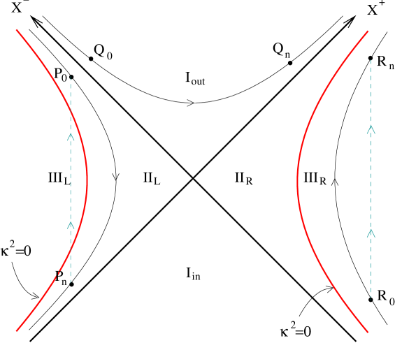
Figure 1: The different space–time regions for the shifted–boost orbifold in $X^{\pm}$–plane. Image points are displaced in the $X$–direction by $2\pi Rn$. All CTC’s must cross region III and none goes into region I. The dashed lines correspond to closed time–like geodesics.

To understand the causal structure in each region of space–time, consider the geodesic distance square between a point with coordinates $X^{a}$ and its $n$–th image, given by

$$8\sinh^{2}(n\pi\Delta)\,X^{+}X^{-}+(2\pi Rn)^{2}\ .$$

Clearly, image points in region I are space–like separated. In region II, provided $n$ is large enough, every point will have a time–like separated image, as shown for points ${\mathrm{P}}_{0}$ and ${\mathrm{P}}_{n}$ in the figure. However, notice that the corresponding geodesic always crosses the $\kappa^{2}=0$ surface. In region III all images are time–like separated. We conclude that there are closed time–like geodesics through regions II and III, which always go through region III. In region I there are no closed time–like geodesics. We shall see below that these results are, in fact, more general, and apply to every causal curve. Thus, if one excises region III from space–time, there will be no closed time–like curves (CTC’s).

Particularly interesting points are those which are light–like related to their $n$–th image. These points lie on the so–called polarization surfaces [65]

$$2X^{+}X^{-}=-\frac{c_{n}}{E^{2}}\ ,\ \ \ \ \ \ \ \ \ \ \ \ \ \ \ \ \ \ c_{n}=\frac{(n\pi\Delta)^{2}}{\sinh^{2}{(n\pi\Delta)}}\ ,$$

which all lie on region II and get arbitrarily close to the horizon for $n\rightarrow\infty$. These surfaces are potentially problematic when one considers loop diagrams in perturbation theory. We shall come back to this issue in section 4.1.

The coordinate transformation such that the Killing vector $\kappa$ becomes trivial is

$$X^{\pm} = y^{\pm}e^{\pm Ez}$$

$$X = z\,.$$

With this coordinate transformation $\kappa=\left(2\pi R\right)\partial_{z}$ and the coordinate $z$ has periodicity $2\pi R$. In order to follow section 2.1, and to write the three–dimensional flat metric in the Kałuża–Klein form in terms of the two–dimensional metric, scalar field and 1–form potential, it is convenient to move to Lorentzian polar coordinates in the $y^{\pm}$–plane. In the Milne wedge, corresponding to the regions I, we choose coordinates

$$y^{\pm}=\frac{t}{\sqrt{2}}\,e^{\pm Ey}$$

and the Kałuża–Klein fields are given

$$\begin{array}[]{c}\displaystyle{ds^{2}=-dt^{2}+\frac{(Et)^{2}}{\Phi^{2}}\,dy^{2}\ ,}\phantom{\framebox{\rule[-11.38092pt]{0.0pt}{0.0pt}}}\\ \displaystyle{\Phi^{2}=1+(Et)^{2}\ ,\ \ \ \ \ \ \ \ A=\left(1-\Phi^{-2}\right)\,dy\ .}\end{array}$$ (8)

We recall that the orbifold has a continuous $U\left(1\right)$ symmetry associated to the Killing vector $\kappa$. Moreover, since $J_{+-}$ and $P_{2}$ commute, one expects a $SO(1,1)$ and a $U(1)$ symmetry. The $SO(1,1)$ corresponds to translations along $y$, and the $U(1)$ to gauge transformations of the 1–form potential.

For $(Et)\ll 1$, the above metric becomes the two–dimensional Milne metric, and therefore ($t=0$, $y\in\left[-\infty,\infty\right]$) is a horizon. For $t\rightarrow\pm\infty$ the geometry becomes flat and space–time decompactifies. Region $\mathrm{I}_{in}$, where $t<0$, is contracting towards a future cosmological horizon, while region $\mathrm{I}_{out}$, where $t>0$, is expanding from a past cosmological horizon. It is natural to ask what happens if one crosses the horizons. This can be done by defining the coordinate transformation that covers regions II and III of the orbifold space

$$y^{\pm}=\pm\frac{x}{\sqrt{2}}\,e^{\pm Ew}\,.$$

Then, the lower dimensional fields read

$$\begin{array}[]{c}\displaystyle{ds^{2}=-\frac{(Ex)^{2}}{\Phi^{2}}\,dw^{2}+dx^{2}\ ,}\phantom{\framebox{\rule[-11.38092pt]{0.0pt}{0.0pt}}}\\ \displaystyle{\Phi^{2}=1-\left(Ex\right)^{2}\ ,\ \ \ \ \ \ \ \ A=\left(1-{\Phi^{-2}}\right)\,dw\ .}\end{array}$$ (9)

Now the geometry is static and for $(Ex)\ll 1$ the metric is just the Rindler metric. Hence, in regions II there is a horizon at ($x=0$, $w\in\left[-\infty,\infty\right]$), that looks just like a black hole horizon. As one moves away from the horizon there is a curvature singularity at $Ex=1$. This singularity corresponds to the surface where the compactification Killing vector $\kappa$ becomes null and region II ends. Behind the singularity the compactification scalar is imaginary because $\kappa$ becomes time–like. It is interesting to compare this with the five–dimensional BMPV black–hole [66]. For this geometry there are also CTC’s which are absent when uplifting the geometry to ten dimensions, however this CTC’s are not hidden behind a singularity of the compactified space [67]. The Carter–Penrose (CP) diagram for this cosmological geometry is shown in figure 2. Two–dimensional cosmological models with similar global structure were also considered in [23, 24]. Immediately one could worry about the instability of the Cauchy horizon when fields propagate from the contracting region. We shall address this delicate issue at the end of this section, but notice that, in contrast with the boost and null–boost orbifolds reviewed below, the compact direction does not shrink to zero size so that classical backreaction may be under control.

Figure 2: CP diagram for the shifted–boost orbifold quotient space. The surface where the Killing vector $\kappa$ is null becomes, in the compactified geometry, a time–like singularity. The future horizon of the contracting region ${\mathrm{I}}_{in}$ is a Cauchy Horizon. Region III is excluded from the diagram.

It is now a simple exercise to show that all closed causal curves passing in regions II must go through the singularity. The proof is identical to the one for the BTZ black hole [68]. Suppose that such a curve exists and has tangent vector

$$l=l^{a}\frac{\partial\ }{\partial x^{a}}\ ,\ \ \ \ \ \ \ \ \ \ x^{a}\equiv(w,x,z)\ .$$

If the curve is closed and time–like in region II there will be a point where $l^{w}=0$. Then the norm of the tangent at this point has to be space–like, as can be seen by the form of the three–dimensional metric in the $x^{a}$–coordinates, which is a contradiction. In order to close the CTC’s one needs to go to regions III, where $z$ becomes the time–like direction. This brings us to an important point. If one excises region III from space–time, the geometry has no CTC’s. However, one needs to justify this procedure and to provide boundary conditions at the naked singularities. When embedded in string theory, we shall see that these singularities behave like mirrors, and therefore the propagation of fields through the geometry is well defined.

2.2.1 Single particle wave functions

Next, let us describe the single particle wave functions on the orbifold. Consider the basis of wave functions that diagonalizes the operators $\square$, $J_{+-}$ and $\kappa$. In the $(t,y,z)$ coordinates these operators have the form

$$\square = -\partial_{t}^{2}-\frac{1}{t}\,\partial_{t}+\frac{1}{(Et)^{2}}\,\partial_{y}^{2}+\left(\partial_{z}-\partial_{y}\right)^{2}\,,$$

$$EJ_{+-} = -i\partial_{y}\,,$$

$$\frac{1}{2\pi i}\,\kappa = -iR\partial_{z}\,,$$

with eigenvalues $m^{2}$, $p$ and $n$, respectively. Omitting the mass label, we start by writing the wave functions as

$$\psi_{p,n}=f(t)\,e^{i\left(py+\frac{n}{R}z\right)}\ .$$

The Klein–Gordon equation then becomes

$$\left[t^{2}\,\frac{d^{2}\ }{dt^{2}}+t\,\frac{d\ }{dt}+(\omega t)^{2}-\nu^{2}\right]\,f(t)=0\ ,$$

where

$$\omega^{2}=m^{2}+\left(p-\frac{n}{R}\right)^{2}\ ,\ \ \ \ \ \ \ \ \ \ \ \ \ \ \ \ \ \ \ \nu=i\,\frac{p}{E}\ .$$ (10)

The function $f(t)$ is a Bessel function of imaginary order $\nu$. Hence, a complete basis for the wave functions in regions I of space–time is given by

$$\psi_{p,n}^{\pm}=J_{\pm\nu}(\omega|t|)\,e^{i\left(py+\frac{n}{R}z\right)}\ .$$ (11)

A similar analysis can be done in regions II, where the wave functions have the form

$$\psi_{p,n}^{\pm}=J_{\pm\nu}(i\omega|x|)\,e^{i\left(pw+\frac{n}{R}z\right)}\ .$$ (12)

These wave functions are defined in each region of space–time. They will be particularly useful to analyze the propagation of fields near the cosmological horizons.

It will be quite useful to express the wave functions as a superposition of the covering space plane waves, and in order to do so we use the general technique of section 2.1. Consider the on–shell plane wave

$$\exp i\left(\pm\frac{\omega}{\sqrt{2}}X^{+}\pm\frac{\omega}{\sqrt{2}}X^{-}+kX\right),$$

with

$$k=\frac{n}{R}-p$$

being the eigenvalue of $P_{2}$. Then it is immediate to use equation (7) to obtain the representation

$$e^{ikX}\int d\sigma\exp i\left(\pm\frac{\omega}{\sqrt{2}}\,e^{\sigma}X^{+}\pm\frac{\omega}{\sqrt{2}}\,e^{-\sigma}X^{-}-\frac{p}{E}\,\sigma\right)$$

$$= e^{i\frac{n}{R}z}\int d\sigma\exp i\left(\pm\frac{\omega}{\sqrt{2}}\,e^{\sigma}y^{+}\pm\frac{\omega}{\sqrt{2}}\,e^{-\sigma}y^{-}-\frac{p}{E}\,\sigma\right)\,.$$

Next, let us consider the above function in region I. It is given by

$$e^{i\left(\frac{n}{R}z+py\right)}\int d\sigma\exp\left(\pm i\omega t\cosh\sigma-i\frac{p}{E}\,\sigma\right)\,.$$

To see that we have obtained the same result as before, we just need to notice that the above integral over $\sigma$ is nothing but the integral representation

$$H_{\nu}^{(1,2)}(x)=\pm\frac{1}{\pi i}\,e^{\mp\frac{i\pi\nu}{2}}\int d\sigma\,\exp\,\left(\pm ix\cosh\sigma-\nu\sigma\right)$$

of the Hankel functions $H_{\nu}^{\left(1,2\right)}$, which are given by specific linear combinations of the Bessel functions.

From the above form of the wave functions, we can anticipate a problem common to all the orbifolds here reviewed [15]. In fact, because these functions have a large UV support on the covering space single particle states, one expects an enhancement of the graviton exchange when they interact gravitationally, which may lead to divergences already at tree level.

2.2.2 Thermal radiation

Let us now move to the analysis of the cosmological particle production, due to the time–dependence of the geometry [22]. The only subtlety here is to define uniquely the transition between particle states in the $\mathrm{I}_{in}$ and $\mathrm{I}_{out}$ vacua. To analyze the behavior of the wave functions $\psi^{\pm}$ defined in (11) and (12) near the horizons, we first recall the expansion of the Bessel functions

$$J_{\nu}(z)=\left(\frac{z}{2}\right)^{\nu}F_{\nu}\left(z^{2}\right)\ ,$$

where $F_{\nu}$ is the entire function

$$F_{\nu}(x)=\sum_{n=0}^{\infty}\,\frac{(-1)^{n}}{4^{n}\,n!\,\Gamma(n+1+\nu)}\,x^{n}\ .$$

The wave function $\psi_{p,n}^{+}$ in the contracting region  I_in becomes $(y^{\pm}<0)$

$$\psi_{p,n}^{+}=\left(\frac{\omega}{\sqrt{2}}\right)^{\nu}\left(-y^{+}\right)^{\nu}F_{\nu}(2\omega^{2}y^{+}y^{-})\,e^{\,i\frac{n}{R}z}\ ,$$

which, near the horizon, behaves like a conformally coupled scalar. As is clear from the above representation, these wave functions can be continued into the intermediate region $\mathrm{II}_{L}$, where $y^{+}<0$ and $y^{-}>0$. Now we come to the delicate issue of boundary conditions at the singularity. We shall argue, in section 4, that the singularity can be understood in string theory as an orientifold plane, where fields obey either Newman or Dirichlet boundary conditions. With this in mind, let us choose for simplicity the Dirichlet boundary conditions, by requiring that the field vanishes at the singularity. This means that we should add, in the region $\mathrm{II}_{L}$, and therefore also in region ${\mathrm{I}}_{out}$, the function

$$-C\,\psi_{p,n}^{-}=-C\left(\frac{\omega}{\sqrt{2}}\right)^{-\nu}\left(y^{-}\right)^{-\nu}F_{-\nu}(2\omega^{2}y^{+}y^{-})\,e^{\,i\frac{n}{R}z}\ ,$$

where $C$ is determined by the boundary condition at $2E^{2}y^{+}y^{-}=-1$ to be

$$C=\left(\frac{\omega}{2E}\right)^{2\nu}\frac{F_{\nu}(-\omega^{2}/E^{2})}{F_{-\nu}(-\omega^{2}/E^{2})}=\frac{J_{ip/E}\left(i\omega/E\right)}{J_{-ip/E}\left(-i\omega/E\right)}\ .$$

Note that $C$ is pure phase, i.e. $C\overline{C}=1$. Physically, the functions $-C\psi^{-}$ can be seen as the reflection of the incident waves $\psi^{+}$ at the singularity, or that, in evolving from region I_in to I_out, one has

$$\psi^{+}\longrightarrow-C\,\psi^{-}\,.$$ (13)

Similarly we have that

$$\psi^{-}\longrightarrow-\overline{C}\,\psi^{+}\,.$$ (14)

We are now ready to determine the Bogoliubov coefficients by considering the full effect of the boundary condition on incoming plane waves in the far past. The functions

$$\begin{array}[]{l}\displaystyle{\mathcal{H}_{p}^{+}=\sqrt{\frac{\pi}{2}}\,\frac{e^{\frac{i\pi}{4}}}{\sinh\left(\pi p/E\right)}\left(e^{\frac{\pi p}{2E}}\,\psi_{p,n}^{+}-e^{-\frac{\pi p}{2E}}\,\psi_{p,n}^{-}\right)\,,}\phantom{\framebox{\rule[-17.07182pt]{0.0pt}{0.0pt}}}\\ \displaystyle{\mathcal{H}_{p}^{-}=\sqrt{\frac{\pi}{2}}\,\frac{e^{-\frac{i\pi}{4}}}{\sinh\left(\pi p/E\right)}\left(-e^{-\frac{\pi p}{2E}}\,\psi_{p,n}^{+}+e^{\frac{\pi p}{2E}}\,\psi_{p,n}^{-}\right)\,,}\end{array}$$ (15)

have the plane–wave asymptotic behavior, for $\left|t\right|\rightarrow\infty$, given by

$$\mathcal{H}_{p}^{\pm}\simeq\frac{1}{\sqrt{\omega\left|t\right|}}\,e^{\pm i\omega\left|t\right|+ipy}\,e^{\,i\frac{n}{R}z}\ ,$$

which follows from the large argument behavior of the Hankel functions. We may then consider, in the far past $Et\ll-1$, the positive frequency plane wave

$$\mathcal{H}_{p}^{-}\simeq\frac{1}{\sqrt{-\omega t}}\,e^{i\left(\omega t+py\right)}\,e^{\,i\frac{n}{R}z}\ .$$ (16)

Using the reflection equations (13) and (14), together with the defining relations (15), the above plane wave will evolve in the future to the following combination of positive and negative frequency waves

$$\alpha\,\,\mathcal{H}_{p}^{+}+\beta\,\mathcal{H}_{p}^{-}\simeq\frac{1}{\sqrt{\omega t}}\left[\alpha\,e^{i\left(pz+\omega t\right)}+\beta\,e^{i\left(pz-\omega t\right)}\right]e^{\,i\frac{n}{R}z}\,,$$

where the Bogoliubov coefficients $\alpha$ and $\beta$ are given explicitly by

$$\alpha=\frac{1}{2i\sinh\left(\pi p/E\right)}\left(e^{-\pi p/E}C-e^{\pi p/E}\,\overline{C}\,\right)\,,$$

$$\beta=\frac{1}{2\sinh\left(\pi p/E\right)}\left(\,C-\overline{C}\,\right)\,.$$

Using the fact that $C\overline{C}=1$, one can easily check that

$$\left|\alpha\right|^{2}-\left|\beta\right|^{2}=1\,.$$

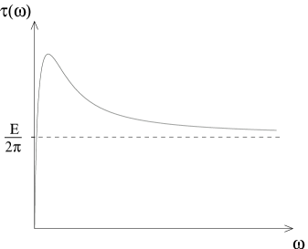
Figure 3: Effective temperature plot for $m=0$. This curve is the cosmological analogue of the Hawking radiation grey body factor for black holes. For massive particles the maximum of the curve is shifted.

The natural choice of the cosmological vacuum is the one defined in the far past $Et\ll-1$ by the plane waves (16). Hence, the observer in the expanding universe will detect an average number $N\left(p\right)$ of particles of momentum $p$ given by the usual formula $N\left(p\right)=\left|\beta\right|^{2}$. Moreover, we can define an effective dimensionless temperature

$$\frac{1}{\tau(\omega)}=\frac{1}{\omega}\,\ln\left|\frac{\alpha}{\beta}\right|^{2}=\frac{2}{\omega}\,\ln\left|\,\frac{e^{-\pi p/E}C-e^{\pi p/E}\,\overline{C}\,}{C-\overline{C}}\right|\ ,$$

which defines particle states with respect to the $\mathrm{I}_{out}$ vacuum. The function $\tau(\omega)$ is plotted in figure 3. Notice that for large $\omega$ one has

$$\tau(\omega)\simeq\frac{E}{2\pi}\ .$$ (17)

Then the physical temperature measured by an observer that is comoving with the expansion in the far future is given by

$$T=\frac{\tau(\omega)}{\sqrt{-g_{tt}}}\ .$$

For the compactification from three to two dimensions associated to the geometry (8) this gives $T=\tau(\omega)$. More generically, when there is an extra conformal factor $\Phi^{2\alpha}$ in the compactified metric, as it is the case in M–theory compactifications, the temperature becomes $T=\tau(\omega)/a(t)$, because asymptotically the scale factor $a(t)$ converges to $\Phi^{\alpha}$. Moreover, since a comoving cosmological observer will measure a red–shifted local energy

$$\Omega=\frac{\omega}{\sqrt{-g_{tt}}}\ ,$$

for fixed $\Omega$, the effective frequency $\omega$ becomes very large and the asymptotic formula for the temperature is

$$T=\frac{E}{2\pi a(t)}\ .$$

This temperature can be interpreted as Hawking radiation due to the presence of a cosmological horizon with non–vanishing surface gravity. In fact, the horizon surface gravity with respect to the Killing vector defined by $\partial_{y}$ in region I and $\partial_{w}$ in region II is $E$. This defines the effective temperature (17) for a state of momentum $p$, which has frequency $\omega$ defined in (10). We shall use this fact in section 4 to generalize the argument for particle production to higher dimensions.

2.2.3 Classical stability of Cauchy horizon

Finally, let us consider the single particle backreaction within the linear regime. The above wave functions are well behaved everywhere except at the horizons $y^{\pm}=0$, where there is an infinite blue–shift of the frequency. To see this, consider the leading behavior of the wave function $\psi_{p,n}^{+}$ as $y^{+}y^{-}\rightarrow 0$

$$\psi_{p,n}^{+}\propto\left|y^{+}\right|^{i\frac{p}{E}}\,e^{\,i\frac{n}{R}z}\ .$$

Near the horizon $y^{-}=0$ the wave function is well behaved and can be trivially continued through the horizon. Near $y^{+}=0$, on the other hand, the wave function has a singularity which can be problematic. In fact, close to the horizon, the derivative $\partial_{+}\psi_{j,n}^{+}\propto\left(y^{+}\right)^{ip/E-1}$ diverges as $y^{+}\rightarrow 0$, and this signals an infinite energy density, since the metric near the horizon has the regular form $ds^{2}\simeq-dy^{+}dy^{-}$. This fact was noted already in [11, 25].

A natural way to cure the problem is to consider wave functions which are given by linear superpositions of the above basic solutions with different values of $p$. The problem is then to understand if general perturbations in the far past $Et\ll-1$ will evolve into the future and create an infinite energy density on the horizon, thus destabilizing the geometry. This problem is well known in the physics of black holes where, generically, Cauchy horizons are unstable to small perturbations of the geometry [69]. Following the work of Chandrasekhar and Hartle for black holes [70], this study was done for cosmologies with a Cauchy horizon in [71, 14]. In particular, in [14], the following was shown. Consider, for simplicity, a perturbation corresponding to an uncharged field of the form $\psi\left(t,y\right)$. At some early time $t_{0}\ll-E^{-1}$, before the field is scattered by the potential induced by the curved geometry, the perturbation is given by a function $\psi\left(t_{0},y\right)=f\left(y\right)$ which is localized in $y$ (for example of compact support or, at most, with a Fourier transform that does not have poles on the strip $|\mathrm{Im}\,p|<E$). Then we can follow the evolution of the field $\psi$ and one discovers that it is perfectly regular at the cosmological horizon. The interested reader can see the details of the computation in [14]. The result is quite different from the case of charged black holes, where the evolution of regular perturbations at the outer horizon produces, quite generally, diverging perturbations at the inner horizon.

2.3 Boost orbifold

The first time–dependent orbifold to be investigated when the subject was revived, was the boost orbifold [9]. It is the $R\rightarrow 0$ limit of the shifted–boost orbifold; however, in this limit, the geometry changes drastically. Space–time points are identified according to

$$X^{\pm}\sim e^{\pm 2\pi\Delta}X^{\pm}\ ,$$

and the spatial $X$–direction plays no role. Each quadrant in the $X^{\pm}$–plane is mapped onto itself, and the origin is a fixed point of the orbifold action. Moreover, points on the light–cone have images arbitrarily close to the origin and, consequently, space–time is not Hausdorff. In figure 4 the orbifold identifications along the orbits of $\kappa$ are represented schematically. This orbifold describes the collision of branes in the ekpyrotic scenario [7]. There, one considers the boost orbifold together with an additional $\mathbb{Z}_{2}$ projection. The orbifold fixed lines are then identified with branes, which are extended along three transverse non–compact space directions, as in the brane world scenario [72].

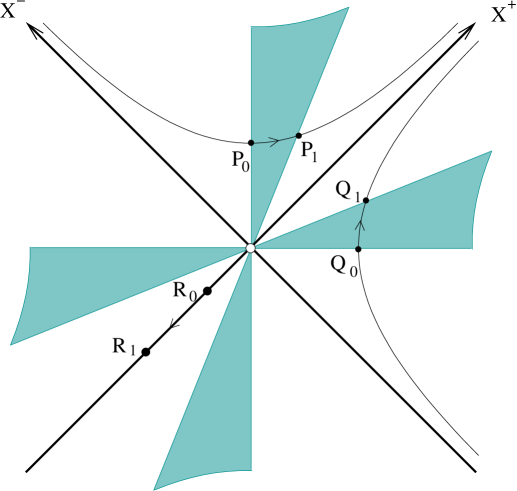
Figure 4: The fundamental domain for the boost–orbifold. There are CTC’s in the whiskers and light–cone points have images arbitrarily close to the origin.

The geodesic distance square between images can be easily computed

$$8\sinh^{2}(n\pi\Delta)\,X^{+}X^{-}\ ,$$

from which we immediately see that there are closed time–like curves (CTC’s) on both left and right quadrants, which are usually called the whiskers.

The coordinate transformation

$$X^{\pm} = \frac{t}{\sqrt{2}}\,e^{\pm\Delta z}$$

$$X = y$$

brings the three–dimensional flat metric to the Kałuża–Klein form

$$ds_{3}^{\,2}=-dt^{2}+dy^{2}+(\Delta t)^{2}dz^{2}\ ,$$

where the $z$–coordinate has periodicity $2\pi$ and the compactification radius varies with time according to $R(t)=2\pi|\Delta t|$. From the original Poincaré invariance on $\mathbb{M}^{2}$, the orbifold breaks translation invariance, but preserves the continuous $SO(1,1)$ associated to translations along the $z$–direction. The CP diagram for the geometry is represented in figure 5.

Figure 5: CP diagram for the boost–orbifold quotient space. Here we consider the covering space $\hbox{\mybb M}^{3}$, but the generalization to higher dimensions is trivial. Only the contracting and expanding regions are represented in this diagram. The remaining regions are the whiskers, which end at the singularity.

The Ricci scalar has a delta function space–like singularity at $t=0$. The initial hope was that, like for the Euclidean $\mathbb{Z}_{N}$ orbifold, string winding states would resolve this singularity. However, as we shall see in section 3.5, the 1–loop partition function for this orbifold has divergences whose physical interpretation remains unclear [19, 20]. This problem is yet to be understood, in particular, the role of the winding states and its relation with the poles of the partition function which originate the above divergence. For recent work on this problem see [21]. This issue is important because it should clarify what is the role of the whiskers, which terminate at the singularity and are not covered by the above coordinate transformation. To embed this construction in M–theory consider the map between the $D=11$ and the type IIA supergravity fields

$$ds_{11}^{\,2}=e^{-\frac{2}{3}\phi}ds_{10}^{\,2}+e^{\frac{4}{3}\phi}\left(dz+A\right)^{2}\ .$$

Then, the orbifold of $\mathbb{M}^{11}$ by a boost gives the type IIA background fields

$$ds^{2}=|\Delta t|\,ds^{2}(\mathbb{M}^{10})\ ,\ \ \ \ \ \ \ \ \ \ \ e^{\phi}=(\Delta t)^{3/2}\ .$$

This geometry describes a universe with a contracting phase for $t<0$ and an expanding phase for $t>0$. At the curvature singularity the string coupling vanishes.

Next let us analyze the single particle wave functions. These can be deduced from the results for the shifted–boost orbifold with little effort by sending $R\rightarrow 0$. The integral representation [20]

$$e^{ikX}\int ds\exp i\left(\pm\frac{\omega}{\sqrt{2}}\,e^{s}X^{+}\pm\frac{\omega}{\sqrt{2}}\,e^{-s}X^{-}-\frac{n}{\Delta}\,s\right),$$

with $\omega^{2}=m^{2}+k^{2}$, defines invariant functions in the full covering space. In particular, in the $X^{\pm}$–plane the functions are nothing but Bessel functions of the radial coordinate with imaginary order $\nu=i\frac{n}{\Delta}$. In the Milne wedge we have the functions

$$J_{\pm i\frac{n}{\Delta}}\left(\omega\left|t\right|\right)\,e^{i\left(ky+\frac{n}{R}z\right)}\,.$$

We wish to consider the problem of particle production. We can follow the same arguments of section 2.2.2, and extend the above functions to the Rindler wedge. This time, though, we do not have a natural boundary where to impose the boundary condition, and we must then impose that the field vanishes at spacial infinity in the whiskers, thus picking the exponentially damped solution [10]. We can then, following again section 2.2.2, define the reflection constant $C$

$$C=\lim_{\eta\rightarrow\infty}\frac{J_{in/\Delta}\left(i\eta\right)}{J_{-in/\Delta}\left(-i\eta\right)}=1\,.$$

The corresponding Bogoliubov coefficients are given by

$$\alpha=i\,,\,\ \ \ \ \ \ \ \ \ \ \ \ \ \ \ \beta=0\,,$$

and we have no particle production. The temperature vanishes. Note that this is not the limit $R\rightarrow 0$ of the results in section 2.2.2, which is, on the other hand

$$C=\lim_{E\rightarrow\infty}\frac{J_{i\left(n/\Delta-k/E\right)}\left(i\sqrt{m^{2}+k^{2}}/E\right)}{J_{-i\left(n/\Delta-k/E\right)}\left(-i\sqrt{m^{2}+k^{2}}/E\right)}\sim\lim_{\eta\rightarrow 0}\frac{J_{in/\Delta}\left(i\eta\right)}{J_{-in/\Delta}\left(-i\eta\right)}\,.$$

The amusing fact is that the above formula still gives $C=1$ for $n=0$, which corresponds to the case considered in [10], by requiring continuity of the wave functions on the covering space. However, for $n\neq 0$ the limit is ill–defined, thus signalling the fact that the $R\rightarrow 0$ limit of the shift–boost orbifold is far more complex than the $R\neq 0$ situation, if the prescription of section 2.2.2 (to be justified in section 4) is correct.

Finally, as for the shifted–boost orbifold, the above single particle wave functions with $n\neq 0$ will induce a large backreaction at the singularity. A simple calculation shows that the corresponding energy density scales near the big crunch/big bang singularity as $t^{-2}$. In this case, however, one can not form a wave packet because the Hankel functions are of discrete order. Physically this problem arises because the compact circle is shrinking to zero size, so that any non–constant perturbation will necessarily induce a large backreaction. In this sense, the addition of a shift to the boost orbifold can be seen as a regulator of the singularity because there is no fixed point.

2.4 $O$–plane orbifold

In section 2.1 we have introduced the $O$–plane orbifold, defined by the Killing vector

$$\kappa=2\pi i\,\left(\Delta\,J_{+2}+R\,P_{-}\right)\,.$$

One can check that, under the action of $e^{\kappa}$, space–time points are identified according to [18]

$$X^{-} \sim X^{-}+2\pi R$$

$$X^{+} \sim X^{+}-(2\pi\Delta)X+\frac{1}{2}\,\left(2\pi\Delta\right)^{2}X^{-}+\frac{1}{6}\,\left(2\pi\right)^{3}R\Delta^{2}$$ (18)

$$X \sim X-(2\pi\Delta)X^{-}-\frac{1}{2}\,\left(2\pi\right)^{2}R\Delta\ .$$

The Killing vector $\kappa$ has norm

$$\kappa^{2}=8\pi^{2}\Delta R\left(X+\frac{1}{2}E\left(X^{-}\right)^{2}\right)\ ,\ \ \ \ \ \ \ \ \ \ \ \ \ \ (E=\Delta/R)\ ,$$

and therefore space–time is naturally divided in two regions, with $\kappa$ space–like or time–like, by the surface

$$X+\frac{1}{2}E\left(X^{-}\right)^{2}=0\ .$$

The geodesic distance square between image points satisfies

$$2E(2\pi Rn)^{2}\left(X+\frac{1}{2}\,E\left(X^{-}\right)^{2}-\frac{1}{12}\,E(2\pi Rn)^{2}\right)\,.$$

Hence, provided $n$ is large enough, points that are in the region where $\kappa$ is space–like are connected to their $n$–th image by a time–like geodesic. Notice, however, that this geodesic always crosses the $\kappa^{2}=0$ surface. More generally, any closed causal curve must cross this surface. This is similar to what happens in regions II and III of the shifted–boost orbifold. In fact this is not a coincidence, since, as we shall see, the $O$–plane orbifold is the limit of the shifted–boost orbifold near the surface where $\kappa$ is null. In figure 6 the identifications on the $X^{-}X$–plane are represented.

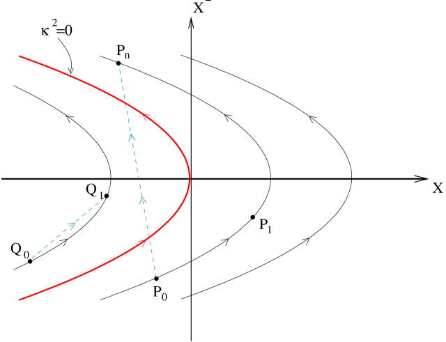
Figure 6: The orbits of the Killing vector $\kappa$ for the $O$–plane orbifold represented in the $X^{-}X$–plane. Image points are displaced in the $X^{+}$–direction according to (18). All CTC’s must cross the region with $\kappa^{2}<0$. The dashed lines represent closed time–like geodesics.

The orbifold breaks the Poincaré invariance of the covering space, and preserves the symmetries generated by $\kappa$ and the translations $P_{+}$ along the $X^{+}$–direction. Also, when embedded in a supersymmetric theory, this orbifold preserves some supersymmetry. Consider, as an example $N=2$, $D=10$ supersymmetry. For the spin structure with periodic boundary conditions on the orbifold circle, supersymmetry transformations generated by spinors satisfying the condition

$$\Gamma^{-}\epsilon=0\ ,$$

are inherited. Thus, this orbifold preserves half of the $N=2$ supersymmetries.

To better study the orbifold geometry, it is very useful to consider the following coordinate transformation

$$X^{-} = y^{-}$$

$$X^{+} = y^{+}-Eyy^{-}+\frac{E^{2}}{6}\left(y^{-}\right)^{3}$$

$$X = y-\frac{E}{2}\left(y^{-}\right)^{2}\,.$$

Then, the flat three–dimensional metric looks like a (trivial) plane wave

$$ds_{3}^{\,2}=-2dy^{+}dy^{-}+2Ey\left(dy^{-}\right)^{2}+dy^{2}\ ,$$

where the $y^{-}$ direction has periodicity $2\pi R$. In terms of the coordinate $y^{a}$, the norm of $\kappa$ is simply$\ 8\pi^{2}\Delta Ry$, so the surface $y=0$ is the locus where the Killing vector $\kappa$ is null. For $y>0$, $\kappa$ is space–like, and for $y<0$, it is time–like. Moreover, the polarization surfaces, where image points are light–like related, are given by $y=E(2\pi Rn)^{2}/12$. If we rewrite the line element in the Kałuża–Klein form

$$ds_{3}^{\,2}=-\frac{\left(dy^{+}\right)^{2}}{2Ey}+dy^{2}+2Ey\,\left(dy^{-}-\frac{dy^{+}}{2Ey}\right)^{2}\ ,$$

we can easily show that it corresponds precisely to the near–singularity limit of the shifted–boost orbifold geometry (9), provided one replaces $y^{+},y^{-}$ by $w,z$ and considers the limit $Ey=|Ex\mp 1|\ll 1$, for $x>0$ or $x<0$, respectively. Thus, the near–singularity limit of the shifted boost orbifold is the $O$–plane orbifold. It then follows that there are CTC’s everywhere, but all these curves must cross the singularity at $y=0$. The CP diagram for this geometry is shown in figure 7.

Figure 7: The CP diagram for the compactified $O$–plane orbifold geometry. The time–like singularity corresponds to the surface $\kappa^{2}=0$ and only the region where $\kappa$ is space–like is represented.

Finally, to find the single particle wave functions, let us choose a basis that diagonalizes the following operators, expressed in the $(y^{\pm},y)$ coordinates,

$$\square = -2\partial_{+}\partial_{-}-2Ey\,\partial_{+}^{\,2}+\partial_{y}^{\,2}\ ,$$

$$P_{+} = -i\partial_{+}\,,$$

$$\frac{1}{2\pi i}\,\kappa = -iR\partial_{-}\,.$$

For a particle of mass $m\,$, the wave functions are labelled by $(p_{+},n)$, and we can use separation of variables to write them as

$$\psi_{p_{+},n}=f(y)\,e^{i\left(p_{+}y^{+}+\frac{n}{R}y^{-}\right)}\ ,$$

where $f(y)$ satisfies the differential equation

$$\left[2\,\frac{n}{R}\,p_{+}+2Ey\,p_{+}^{\,2}+\frac{d^{2}\ }{dy^{2}}-m^{2}\right]\,f(y)=0\ .$$

Defining the new variable

$$\omega=-\left(2Ep_{+}^{\,2}\right)^{\frac{1}{3}}\left(y+\frac{n}{ERp_{+}}-\frac{m^{2}}{2Ep_{+}^{\,2}}\right)\ ,$$

the above differential equation simplifies to

$$\frac{d^{2}f}{d\omega^{2}}=\omega\,f\ ,$$

which describes, in quantum mechanics, a zero energy particle subject to a linear potential. The solutions are the Airy functions $Ai(\omega)$ and $Bi(\omega)$, which are, respectively, exponentially damped or exponentially growing in the $\omega>0$ region. This region corresponds mostly to negative $y$, where the Killing vector $\kappa$ is time–like. Choosing the normalizable solution, we have just shown that

$$\psi_{p_{+},n}\propto Ai(\omega)\,e^{i\left(p_{+}y^{+}+\frac{n}{R}y^{-}\right)}.$$

This choice has a clear physical interpretation. Consider a particle of mass $m$ and Kałuża–Klein charge $n$. Since the Airy function $Ai(\omega)$ and its derivative are exponentially damped for $\omega<0$, the probability of finding the particle in the region

$$y<y_{c}=\frac{m^{2}}{2Ep_{+}^{\,2}}-\frac{n}{ERp_{+}}\ ,$$

is negligible. This behavior is clear physically: in the covering space, all time–like geodesics that go through the region $y<0$ remain there for a finite proper time, explaining why the wave function is damped. Moreover, for very large $p_{+}$, the particle gets arbitrarily close to the singularity. Finally, the case of charged particles is particularly interesting, since $y_{c}$ is linear with$\,n$. Particles with positive charge are attracted towards the singularity, whereas negatively charged particles are repelled.

We shall now obtain an integral representation of the function $\psi_{p_{+},n}$, as a superposition of standard plane waves in the covering space. We start from the integral representation of the Airy function

$$Ai(\omega)=\frac{1}{2\pi}\int dt\,\,e^{\,i\left(\omega t+\frac{t^{3}}{3}\right)}\ ,$$

which immediately yields

$$\psi_{p_{+},n}\propto\,e^{i\left(p_{+}y^{+}+\frac{n}{R}y^{-}\right)}\int ds\,e^{i\left(y+\frac{n}{ERp_{+}}-\frac{m^{2}}{2Ep_{+}^{\,2}}\right)s-\frac{i}{6}\frac{s^{3}}{Ep_{+}^{2}}}\,.$$

Changing coordinates to the original Minkowski coordinates $X^{a}$, and defining the new integration variable $p=s+X^{-}p_{+}E$, one gets after choosing a specific normalization

$$\psi_{p_{+},n}=\frac{1}{\sqrt{\left|p_{+}\right|}}\int dp\,\,\phi_{p_{+},p}\left(X\right)\,\,\exp\frac{i}{E}\left(\frac{np}{Rp_{+}}-\frac{1}{2}\frac{m^{2}p}{p_{+}^{\,2}}-\frac{1}{6}\frac{p^{3}}{p_{+}^{\,2}}\right)\ ,$$ (19)

where

$$\phi_{p_{+},p}\left(X\right)=\,e\,^{i\left(p_{+}X^{+}+p_{-}X^{-}+pX\right)}\ ,\ \ \ \ \ \ \ \ \ \ \ \ p_{-}=\frac{m^{2}+p^{2}}{2p_{+}}\ ,$$

is the usual on–shell flat space plane wave. The integral representation (19) is nothing but the representation described in general in section 2.1, as it is possible to show starting from the identifications (18). We leave this check to the interested reader. It is a matter of computation to show that the above single–particle functions satisfy the orthogonality condition

$$\langle m^{2},p_{+},n|m^{\prime 2},p_{+}^{\prime},n^{\prime}\rangle=32\pi^{4}ER\,|p_{+}|\,\delta\left(m^{\,2}-m^{\prime\,2}\right)\delta\left(p_{+}-p_{+}^{\prime}\right)\delta_{n-n^{\prime}}\ ,$$ (20)

where we have reinserted the mass label.

Finally, since $\partial_{+}$ is a globally defined null Killing vector these functions define the same particle states in the $y_{+}\rightarrow\pm\infty$ regions. Consequently, it is possible to define a global vacuum and there is no particle production.

2.5 Null–boost orbifold

The null–boost orbifold was studied recently in [28, 15]. To obtain the identification of space–time points for this orbifold, we can simply set $R=0$ in the analogous equation (18) for the $O$–plane orbifold

$$X^{-} \sim X^{-}$$

$$X^{+} \sim X^{+}-(2\pi\Delta)X+\frac{1}{2}\,\left(2\pi\Delta\right)^{2}X^{-}$$

$$X \sim X-(2\pi\Delta)X^{-}\,.$$

The Killing vector $\kappa=2\pi i\,\Delta\,J_{+2}$ is everywhere space–like except at $X^{-}=0$, where it is null. Moreover, $\kappa$ vanishes on the $X^{+}$–axis ($X^{-}=X=0$), which is a fixed line of the orbifold. The geodesic distance square between image points is

$$(2\pi\Delta nX^{-})^{2}\ ,$$

which vanishes on the surface $X^{-}=0$. Hence, there will be closed null curves (CNC’s) on this surface. The orbifold action is represented schematically on the $X^{-}X$–plane in figure 8. This orbifold preserves the symmetries generated by $J_{+2}$ and $P_{+}$, and also the same supersymmetries of the $O$–plane orbifold.

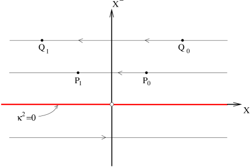
Figure 8: The orbits of the Killing vector $\kappa$ for the null–boost orbifold represented in the $X^{-}X$–plane. Image points are displaced in the $X^{+}$–direction according to (2.5). There are CNC’s on the surface $X^{-}=0$ and the origin is a fixed point.

The coordinate transformation

$$X^{-} = y^{-}$$

$$X^{+} = y^{+}+\frac{\Delta^{2}}{2}\,z^{2}y^{-}$$

$$X = \Delta zy^{-},$$

brings the three–dimensional flat metric to the form ($z\sim z+2\pi$)

$$ds_{3}^{2}=-2dy^{-}dy^{+}+(\Delta y^{-})^{2}dz^{2}\ ,$$

so that the compact circle has radius $R(y^{-})=2\pi|\Delta y^{-}|$. This metric describes a dilatonic wave that is singular at $y^{-}=0$. This is where the orbifold action is fixed and where the energy density of infalling matter will diverge, leading to a large backreaction. The CP diagram for this geometry is shown in figure 9.

Figure 9: The CP diagram for the compactified null–boost orbifold geometry. The null–like singularity corresponds to the surface where $\kappa$ is null and where the CNC’s are.

The wave functions for this orbifold can be obtained from (19) by setting $R=0$. This gives [15]

$$\psi_{p_{+},n}=\frac{1}{\sqrt{\left|p_{+}\right|}}\int dp\,\ \phi_{p_{+},p}\left(X\right)\,\ e^{\,i\frac{np}{\Delta p_{+}}}\ .$$

The $p$–integral is gaussian and can be explicitly done to obtain

$$\psi_{p_{+},n}=\sqrt{\frac{2\pi i}{\left|X^{-}\right|}}\,\exp i\left[\frac{m^{2}}{2p_{+}}X^{-}+p_{+}X^{+}-\frac{p_{+}}{2X^{-}}\left(X+\frac{n}{\Delta p_{+}}\right)^{2}\right].$$

In the limit $X^{-}\rightarrow 0$ the wave functions become singular. More precisely,

$$\lim_{X^{-}\rightarrow 0}\psi_{p_{+},n}=2\pi\,\sqrt{\frac{i}{\left|p_{+}\right|}}\,\delta\left(X+\frac{n}{\Delta p_{+}}\right)\,e^{i\,p_{+}X^{+}}\ .$$

Thus, the wave functions are focused on the lattice $X\in\left(\Delta p_{+}\right)^{-1}\mathbb{Z}$. This divergence is not integrable because $n$ is discrete and, consequently, these particle states create a large backreaction on the geometry. Notice that $n/\Delta$ is the eigenvalue of $J_{2+}$, which is forced to be have discrete eigenvalues.

For the null–brane [16, 63], where the orbifold generator includes a translation $P_{3}$ along an extra spatial direction, a similar focusing occurs, at $X=-J_{2+}/p_{+}$. On the other hand, now, since only $\Delta J_{2+}+RP_{3}\in\mathbb{Z}$, and since $P_{3}$ has continuous spectrum, so does $J_{2+}$. Therefore we have a continuum of focusing points, and by choosing wave–packets which are linear combinations with different values of $J_{2+}$, we can construct regular wave–packets in both the covering and the quotient space. As we shall see in the next section, perturbation theory is badly behaved in the case of both the null–boost and the $O$–plane orbifold. In [16] the authors show that, on the other hand, perturbation theory is well–behaved in the case of the null–brane, and they claim that this is due to the possibility of constructing regular single particle states, as we have just discussed. This claim is clearly not correct, since the $O$–plane orbifold has perfectly regular wave–functions, but suffers from the same pathology of the null–boost case.

3 Interactions

So far we have reviewed in detail the geometry and the single particle wave functions for the time–dependent orbifolds of three–dimensional flat space. The next natural step is to consider interactions. In fact, the same phenomenon that leads to the blue–shift of single particle states during a cosmological contracting phase, could give rise to instabilities due to particle interactions. Physically, the acceleration induces a stronger coupling to the graviton, enhancing the exchange of this particle. One way to see this is given by the argument, put forward by Horowitz and Polchinski [12], for the formation of large black holes. We shall review this argument below and comment on its regime of validity and limitations. A more precise analysis can be done, in three dimensions, using the powerful techniques of two–dimensional dilaton gravity, which permits an exact study of conformal matter propagating in the quotient space of the previously described orbifolds [13, 14]. Another way to study particle interactions, which does not always gives the same result regarding stability, is by direct computation of tree level amplitudes [15, 16, 17]. We shall review how divergences are found in four–point amplitudes, and how these amplitudes can be made finite by resumming generalized ladder graphs in the eikonal approximation [18]. One–loop amplitudes will also be reviewed [19, 20, 15], together with on–shell winding states wave functions [21].

3.1 Formation of large black–holes

It has been argued, in [12], that a large class of time–dependent orbifolds are unstable to small perturbations, due to a large backreaction of the geometry. These results do not rely on string theory arguments, and are obtained within the framework of classical General Relativity. The argument is quite simple and starts by consider a particle in the orbifold geometry, which corresponds to an infinite collection of particles in the covering space. If the interaction between image particles produces a black hole in the covering space, then this signals that a black hole is formed in the orbifold quotient space. The condition for black hole formation in the covering space is that, given a particle and its $n$–th image, their impact parameter $b$ should be smaller than the Schwarzchild radius associated to the center of mass energy $\mathcal{E}$,

$$G\mathcal{E}>b^{D-3}\ ,$$

where $D$ is the dimension of space–time. In practice, one is interested in interactions with large boosted images, so that one can consider, without loss of generality, particles moving along null geodesics. The condition for black hole formation can then be made quite precise, because it corresponds to the existence of a trapped surface in space–time when two shock–waves, described by the Aichelberg–Sexl metrics [73], collide [74].

Let us now be more quantitative and consider a null geodesic with world–line

$$X^{a}(\lambda)=p^{a}\lambda+C^{a}\ ,$$

where $p^{a}$ is the momentum and $C^{a}$ a point along the geodesic. The $n$–th image geodesic has world–line

$$X_{n}^{\,a}(\lambda)=p_{n}^{\,a}\lambda+C_{n}^{\,a}\ ,$$

where $p^{a}_{n}$ and $C^{a}_{n}$ are the images, under the orbifold action $e^{n\kappa}$, of the momentum $p^{a}$ and of the point $C^{a}$, respectively. Simple kinematics shows that the impact parameter $b$ and center of mass energy $\mathcal{E}$ are given by

$$b^{\,2}=Y^{\,2}-\frac{2(p\cdot Y)(p_{n}\cdot Y)}{p\cdot p_{n}}\ ,\ \ \ \ \ \ \ \ \ \mathcal{E}^{2}=-2p\cdot p_{n}\ ,$$

where $Y=C-C_{n}$.

It is now a mater of computation to determine which orbifolds are stable or unstable according to these criteria. Consider, as an example, the $O$–plane orbifold. Let $p^{a}$ and $C^{a}$ be given by

$$p=\left(\begin{array}[]{c}p^{+}\\ p^{-}\\ p\\ \vec{p}_{\perp}\end{array}\right)\ ,\ \ \ \ \ \ \ \ \ C=\left(\begin{array}[]{c}C^{+}\\ 0\\ C\\ \vec{C}_{\perp}\end{array}\right)\ ,$$

where we allowed for possible extra spectator directions, and where we parametrize the null geodesic so as to set $C^{-}=0$ (the case when $p^{-}=0$ implies that $p^{a}$ and $p_{n}^{a}$ are collinear, with $\mathcal{E}=0$ and no black–hole formation). Then the momentum of the $n$–th image particle reads

$$p_{n}=\left(\begin{array}[]{c}\displaystyle{p^{+}-\beta p+\frac{\beta^{2}}{2}\,p^{-}}\\ p^{-}\\ p-\beta p^{-}\\ \vec{p}_{\perp}\end{array}\right)\ ,$$

where $\beta=2\pi n\Delta$ and the constant $Y$ satisfies

$$EY=\left(\begin{array}[]{c}\displaystyle{-\beta EC+\frac{1}{6}\,\beta^{3}}\phantom{\framebox{\rule[-5.69046pt]{0.0pt}{0.0pt}}}\\ \displaystyle{\beta}\phantom{\framebox{\rule[-5.69046pt]{0.0pt}{0.0pt}}}\\ \displaystyle{-\frac{1}{2}\,\beta^{2}}\phantom{\framebox{\rule[-8.5359pt]{0.0pt}{0.0pt}}}\\ \vec{0}\end{array}\right)\ .$$

Finally, for large $n$, the impact parameter and the center of mass energy are

$$b\simeq\frac{2}{3}\,R\Delta(\pi n)^{2}\ ,\ \ \ \ \ \ \ \ \ \ \ \ \ \mathcal{E}\simeq|p^{-}|2\pi\Delta n\ ,$$

and we conclude that the $O$–plane orbifold is stable, according to this criteria.

For the null–boost orbifold, start by setting $R=0$ (or $E\rightarrow\infty$) in the above expressions for the momenta $p_{n}$ and constant $Y$. Then one obtains that the large $n$ behavior for the center of mass energy remains unchanged, while the impact parameter becomes $b\simeq 2C$. Hence, the null–boost orbifold is unstable. In the case of the null–brane, where one adds a translation to the null–boost orbifold action in a direction orthogonal to the $\mathbb{M}^{3}$, again $\mathcal{E}$ is unchanged but $b\simeq 2\pi Rn$. In this case, provided $D\geq 5$, black holes do not form. The cases of the boost and shifted–boost orbifolds can be analyzed in a similarly way. One obtains that $b$ is polynomial in $n$, while $\mathcal{E}$ grows exponentially, with the result that both are unstable. In table 2 we give a summary of the results.

Table 2: Horowitz–Polchinski analysis for the time–dependent orbifolds of $\hbox{\mybb M}^{3}$.

Orbifold	$b$	$\mathcal{E}$	Result
Boost	$\phantom{\framebox{\rule[-11.38092pt]{0.0pt}{0.0pt}}}\displaystyle{\sqrt{\frac{2p^{-}}{p^{+}}}\,|C^{+}|}\phantom{\framebox{\rule[19.91684pt]{0.0pt}{0.0pt}}}$	$\sqrt{2p^{+}p^{-}}e^{\pi\Delta n}$	Unstable
Shifted–boost	$\phantom{\framebox{\rule[-2.84544pt]{0.0pt}{0.0pt}}}2\pi Rn\phantom{\framebox{\rule[8.5359pt]{0.0pt}{0.0pt}}}$	$\sqrt{2p^{+}p^{-}}e^{\pi\Delta n}$	Unstable
Null–boost	$\phantom{\framebox{\rule[-2.84544pt]{0.0pt}{0.0pt}}}2C\phantom{\framebox{\rule[8.5359pt]{0.0pt}{0.0pt}}}$	$|p^{-}|2\pi\Delta n$	Unstable
$O$–plane	$\phantom{\framebox{\rule[-8.5359pt]{0.0pt}{0.0pt}}}\displaystyle{\frac{2}{3}\,(\pi n)^{2}\Delta R}\phantom{\framebox{\rule[14.22636pt]{0.0pt}{0.0pt}}}$	$|p^{-}|2\pi\Delta n$	Stable

This stability argument should be taken with some criticism. In fact, it seems unlikely that a correct guess on the final qualitative features of the scattering problem can be obtained by looking at the interaction between two (or, for that matter, a finite number of) light–rays. This fact is already true if we just consider the linear reaction of the gravitational field to the image geodesics. Then, very much like in electromagnetism, it is incorrect to guess the qualitative features of fields by looking at just a finite subset of the charges (matter in this case), whenever the charge distribution is infinite (this infinity is really not an approximation in this case, since it comes from the infinite copies of the particle in the covering space). In particular, it was shown in [75] that, for the boost orbifold with four extra non–compact directions, the linear gravitational field produced by all the images is pure gauge. Therefore, to decide if the problem exists, much more work is required, already in the linear regime of gravity, but most importantly in the full non–linear setting. Also, we saw that, according to this argument, the $O$–plane orbifold is stable. We shall see, on the other hand, that it suffers from the same infinities in the two–particles scattering amplitudes found in [15], questioning the agreement between the two approaches.

Finally, notice that the only case in which the HP argument is fully correct is exactly in dimension $D=3$, where the gravitational interaction is topological and when, therefore, the interaction of an infinite number of charges can be consistently analyzed by breaking it down into finite subsets. This indeed is what we shall find in the next section.

3.2 Backreaction in three–dimensions

As we have described in the last section, it is quite important to understand the full non–linear response of the orbifold geometry due to small perturbations. Fortunately, at least in three dimensions, the problem can be solved exactly for a specific type of matter fields. The reason is that the orbifold geometry is described by two–dimensional dilaton gravity. Then, for conformally coupled matter, one can derive the full non–linear solution, including the backreaction of the conformal field. We shall consider the null–boost and the shifted–boost orbifolds in some detail, and we shall ask if conformal matter gives rise to a space–like singularity, changing abruptly the space–time global structure. Notice that the analysis of the shifted–boost orbifold includes the $O$–plane orbifold if one takes the near–singularity limit.

Recall the general form for the dimensional reduction of the three-dimensional metric

$$ds_{3}^{\,2}=ds_{2}^{\,2}+\Phi^{2}\left(dz+A\right)^{2}\ ,$$

where $\partial_{z}$ is a Killing direction. The three–dimensional Hilbert action is proportional to

$$\int d^{2}x\,\sqrt{-g}\left(\Phi R-\frac{1}{2}\,\Phi^{3}F^{2}\right)\ .$$

The equation of motion for the gauge field implies that the scalar $\Phi^{3}\star F$ is constant. By rescaling $z$, $A$ and $\Phi^{-1}$ we can fix the constant to any desired value (provided it does not vanish) so that $\star F=2/\Phi^{3}$. This will be possible for the $O$–plane and for the shift–boost orbifold. On the other hand, $F=0$ for the boost and the null–boost orbifolds. Focusing, for now, on the case $F\neq 0$, the equations of motion for the scalar $\Phi$ and the metric can be derived from the action

$$\int d^{2}x\left(\Phi R-V(\Phi)\right)\ ,\ \ \ \ \ \ \ \ \ V(\Phi)=\frac{2}{\Phi^{3}}\ .$$

We conclude that the problem of finding the geometry for the orbifolds of $\mathbb{M}^{3}$ can be rephrased in the language of two–dimensional gravity. Note that, in this theory, the metric and the scalar $\Phi$ should be considered together as the gravitational sector.

Next we wish to add the matter sector, which results in an action of the general form

$$S_{2D}(g,\Phi)+S_{M}(g,\Phi,\mathrm{Matter})\ .$$

The corresponding equations of motion are easily derived to be

$$\begin{array}[]{rcl}\displaystyle{2\nabla_{a}\nabla_{b}\Phi}&=&\displaystyle{g_{ab}\left(2\,\Box\Phi+V\right)-\tau_{ab}\,}\ ,\phantom{\framebox{\rule[-11.38092pt]{0.0pt}{0.0pt}}}\\ R&=&\displaystyle{\frac{dV}{d\Phi}+\rho}\ ,\end{array}$$

where $\tau_{ab}$ and $\rho$ are

$$\tau_{ab}=-\frac{2}{\sqrt{-g}}\frac{\delta S_{\mathrm{M}}}{\delta g^{ab}}\ ,\ \ \ \ \ \ \ \ \ \ \ \ \ \ \ \ \ \ \ \ \ \ \ \rho=-\frac{1}{\sqrt{-g}}\frac{\delta S_{\mathrm{M}}}{\delta\Phi}\ .$$

Moreover, the conservation of the stress energy tensor $\tau_{ab}$ is modified by the dilaton current $\rho$ to

$$\nabla^{a}\tau_{ab}+\rho\nabla_{b}\Phi=0\ .$$

The inherent simplicity of the dilaton gravity model lies in the following observations [76, 77]. Define $J\left(\Phi\right)$ by

$$J=\int Vd\Phi$$

and consider the function

$$C=\left(\nabla\Phi\right)^{2}+J\left(\Phi\right)$$ (21)

and the vector field

$$\kappa^{a}=\frac{2}{\sqrt{g}}\,\epsilon^{ab}\,\nabla_{b}\Phi\ .$$

Then, for any vacuum solution $\tau_{ab}=\rho=0$, the function $C$ is constant and $\kappa$ is a Killing vector. The first fact follows from the equations of motion, which imply that

$$\nabla_{a}C=-\tau_{ab}\nabla^{b}\Phi+\nabla_{a}\Phi\,(\tau_{bc}g^{bc})\ .$$ (22)

The second fact is proved most easily in conformal coordinates $z^{\pm}$, with metric

$$-dz^{+}dz^{-}e^{\Omega}\ .$$

Then $\kappa_{\pm}=\mp\nabla_{\pm}\Phi$, and the non–trivial Killing equations become $\nabla_{+}\nabla_{+}\Phi=\nabla_{-}\nabla_{-}\Phi=0$, which hold whenever $\tau_{ab}=0$. Finally note that these equations are equivalent to

$$\partial_{-}\kappa^{+}=\partial_{+}\kappa^{-}=0\ .$$

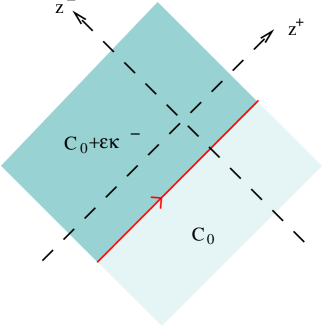
Figure 10: Shock wave solution in two–dimensional dilaton gravity.

Let us now analyze the geometry in the presence of matter. For our purposes, we are going to consider only matter Lagrangians which do not depend on the dilaton, and which are conformal. This implies that

$$\begin{array}[]{c}\tau_{+-}=\rho=0\ ,\\ \partial_{-}\tau_{++}=\partial_{+}\tau_{--}=0\ .\end{array}$$

The simplest example is clearly a conformally coupled scalar $\eta$ with $S_{M}=-\int\left(\nabla\eta\right)^{2}$. The effect of this type of matter is best described by considering a shock wave [78], which is represented in conformal coordinates by a stress energy tensor of the form

$$\tau_{--}\left(z^{-}\right)=\epsilon\,\delta\left(z^{-}-z_{0}^{-}\right)\ ,\ \ \ \ \ \ \ \ \ \ \ \ \ \ \ \ \ \ \ \ \ \ \ \ \left(\epsilon>0\right)\,.$$

The positivity of $\epsilon$ can be understood by looking at the conformally coupled scalar, for which $\tau_{--}=2\left(\nabla_{-}\eta\right)^{2}>0$. Recalling from (22) that

$$\nabla_{-}C=2\tau_{--}\nabla_{+}\Phi\,e^{-\Omega}=\tau_{--}\kappa^{-}\,,$$ (23)

we conclude that the shock front interpolates, as we move along $z^{-}$, between the vacuum solution with $C=C_{0}$ and the vacuum solution with $C=C_{0}+\epsilon\kappa^{-}(z_{0}^{-})$ (see figure 10). As a consistency check note that, since in the vacuum $\tau_{--}$ and $\kappa^{-}$ are functions only of $z^{-}$, equation (23) defines a jump in the function $C$ which is independent of the position $z^{+}$ along the shock wave.

We are now in a position to study the coupling of conformal matter to the orbifolds geometry, including non–linear effects. Consider first the case of the shifted–boost orbifold [14]. It is easy to verify that the corresponding geometry corresponds to a constant $C$ given by

$$C=-E\ .$$

For example, in the static regions II one has

$$\begin{array}[]{rcl}ds_{2}^{\,2}&=&\displaystyle{-dt^{2}\left(\frac{E^{2}x^{2}}{1-E^{2}x^{2}}\right)+dx^{2}}\ ,\phantom{\framebox{\rule[-11.38092pt]{0.0pt}{0.0pt}}}\\ \sqrt{E}\,\Phi&=&\displaystyle\sqrt{1-E^{2}x^{2}}\ .\end{array}$$ (24)

Note that we have rescaled the field $\Phi$ from section 2.2 in order to have a canonically normalized potential $2\Phi^{-3}$. Given the parameter $E$, one has no freedom in the solution, which is unique. This shows that there is no fine tuning in the choice of initial conditions for the metric and the dilaton, in order to obtain a bounce cosmological solution with past and future cosmological horizons.

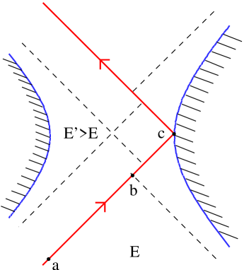
Figure 11: Shock wave solution in the cosmological geometry associated to the shifted–boost orbifold.

Next we add matter by considering shock wave solutions. Given the above discussion, it is immediate to see that, after the wave, one has again a vacuum solution, but with a different constant

$$E^{\prime}=E-\epsilon\kappa^{-}\ ,$$

where $\epsilon>0$ and $\kappa^{-}=2e^{-\Omega}\nabla_{+}\Phi$ must be computed along the wave. In figure 11 the new geometry is represented. As one moves in this figure from point $a$ to points $b$ and $c$ along the shock wave, in the direction of increasing $z^{+}$, the value of $\Phi$ decreases to $0$ at $c$ on the singularity. Therefore $\nabla_{+}\Phi<0$ and one has that

$$E^{\prime}>E\ .$$

Moreover, in any vacuum solution with $C=-E$, the value of the dilaton on the horizons is $1/\sqrt{E}$, as can be seen from equation (24) at $x=0$. Therefore, since the value of $\Phi$ is continuous across the shock wave, the horizon to the left of the wave, where the dilaton has value $\Phi=1/\sqrt{E^{\prime}}$, must intersect the wave between the points $b$ and $c$, as drawn. Let us briefly explain why the horizon at a constant value of $z^{+}$ shifts as one passes the shock wave. It is easy to see that the horizon in question is given by the curve $\kappa^{+}=0$. In the vacuum, $\kappa^{+}$ is a function of $z^{+}$ alone, but in the presence of matter one has that

$$\partial_{-}\kappa^{+}=e^{-\Omega}\tau_{--}\,.$$

Then, since $\Omega$ is constant along the horizons (and therefore along the shock wave) and since $\tau_{--}$ has a delta singularity, the function $\kappa^{+}$ just jumps by a finite constant across the wave, thus explaining the shift in the position of the horizon.

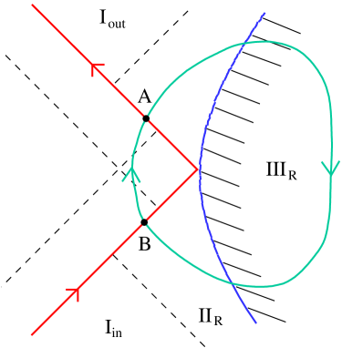
Figure 12: A closed time–like curve in the three–dimensional geometry induced by the matter surface, which is the oxidization of the shock front.

In conclusion, for the shifted–boost orbifold, the addition of matter does not change the global structure of space–time, because the solution interpolates between two non–BPS vacua with the same global structure. In particular, there is no space–like singularity leading to a catastrophic big–crunch. Is this result in contradiction with the argument reviewed in the previous section? The answer is no. To see this consider the uplift to three dimensions of the shock front geometry. It is given by two pieces of flat space separated by a surface of matter. This distribution of matter is nothing but the continuous image of a light ray generated by the action of the orbifold Killing vector. Then a simple generalization of the argument for the formation of large–black holes to continuous surfaces leads to the same instability as before. However, in three–dimensional gravity there are no black holes, a fact that follows simply because $GM$ is dimensionless. In this case, the instability analogous to the formation of black holes is the appearance of CTC’s in the covering space [79, 80, 81, 82]. In fact, given a two particle scattering process, the instability condition in three dimensions

$$G\mathcal{E}>1\ ,$$

becomes the condition for the formation of CTC’s. A careful analysis of the covering space geometry corresponding to the shock front geometry, indeed shows that such CTC’s do appear, and there is no contradiction. However, all these covering space CTC’s cross the surface that corresponds to the time–like singularities of regions II. Such a closed time–like curve is represented in the compactified space in figure 12. Provided one interprets the singularities as boundaries of space–time, and accordingly excises from the geometry the region behind it, one concludes that the final geometry is free of CTC’s and the above instability is cured.

Let us now consider the case of the null–boost orbifold. Lawrence analyzed the reaction of the geometry when conformally coupled matter strikes the null singularity [13]. In this case, however, an instability is found, which indicates a behavior already expected from the limiting form of the wave functions at the big–crunch singularity. The problem can again be rephrased in the language of two–dimensional dilaton gravity, but now in a theory with a vanishing dilaton potential. The vacuum null–boost geometry is the $C=0$ solution, which is supersymmetric. When one introduces a shock wave heading towards the singularity, the constant $C$ will become negative and one connects, after the shock wave, to the non–supersymmetric pure boost space–time. The latter geometry has a totally different global structure, as we saw in section 2, with a space–like singularity corresponding to the big crunch. In figure 13 the CP diagram representing the gluing of both geometries across the shock wave is shown.

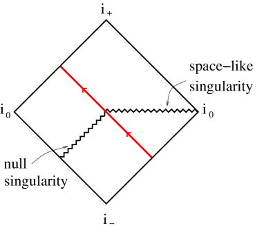
Figure 13: CP diagram for the shock wave solution in the null–boost geometry.

Finally, if one considers perturbing the pure boost geometry with a shock wave, one does not expect drastic changes of space–time structure, since one interpolates, across the shock, between two non–BPS geometries with equal global structure.

3.3 Tree–level Amplitudes

In this section we concentrate on the computation of tree–level amplitudes of field theory and string theory on the orbifolds $(\mathbb{M}^{3}/e^{\kappa})\mathbb{\times T}^{D-3}$, where $D$ is the space–time dimension. The basic tool used to compute these amplitudes is the inheritance principle, which states that we may use directly the amplitudes of the parent theory on $\mathbb{M}^{3}\mathbb{\times T}^{D-3}$, as long as we restrict our attention to external states which are invariant under the orbifold action. This principle is certainly valid in field theory, and is also the correct prescription for string states which do not carry winding charge. For concreteness of exposition, we shall consider only the $O$–plane orbifold [18], but notice that similar techniques have been used for other orbifolds discussed in these lectures: the amplitudes for the null–boost and null–brane, which can be derived easily from the computation here presented, were considered in [15, 16] and for the boost–orbifold in [17].

Let us discuss first, in general, the $n$–point amplitude and then restrict our attention to $n=3,4$. Let the parent amplitude be given by

$$\delta^{3}\left(\mathop{\textstyle\sum}\nolimits_{i}\vec{p}_{i}\right)\mathcal{A}\left(\vec{p}_{1},\cdots,\vec{p}_{n}\right)\,,$$

where the momenta $\vec{p}_{i}$ refer to the momenta in the $\mathbb{M}^{3}$ directions . We will consider as given, once and for all, the discrete momenta $\vec{p}_{i\perp}$ in the torus directions $\mathbb{T}^{D-3}$, with the only obvious requirement that $\sum_{i}\vec{p}_{i\perp}=0$.

As we saw in section 2.3, the external states are characterized by their mass $m_{i}$, together with the conserved quantum numbers $(p_{i+},n_{i})$. Moreover, the mass is clearly related to the $D$–dimensional mass $M_{i}^{\,2}$ by

$$m_{i}^{\,2}=M_{i}^{\,2}+(\vec{p}_{i\perp})^{2}\,.$$

Using the basic external states (19), we may directly apply the inheritance principle to obtain the expression

$$\frac{1}{\sqrt{\left|\prod_{i}p_{i+}\right|}}\int dp_{1}\cdots dp_{n}\,\delta\left(\mathop{\textstyle\sum}\nolimits_{i}p_{i+}\right)\delta\left(\mathop{\textstyle\sum}\nolimits_{i}p_{i}\right)\delta\left(\mathop{\textstyle\sum}\nolimits_{i}p_{i-}\right)e^{i\varphi\left(p_{i}\right)}\,\mathcal{A}\left(\vec{p}_{i}\right)\ .$$ (25)

As we just mentioned, the momenta $p_{i+}$ are fixed. On the other hand, the momenta $p_{i}$, which are momenta in the $X$–direction, are integrated and the momenta $p_{i-}$ are given by the quadratic on–shell condition

$$p_{-}=\frac{p^{2}+m^{2}}{2p_{+}}\,.$$

Therefore, of the three delta functions, the one related to the $X^{+}$–direction factors out of the integral, whereas the ones related to the directions $X$ and $X^{-}$ give, respectively, a linear and a quadratic constraint on the integration variables $p_{i}$. Finally, the phase $\varphi\left(p_{i}\right)$ is given by

$$\varphi\left(p_{i}\right)=\frac{1}{E}\sum_{i}\left(\frac{p_{i}n_{i}}{Rp_{i+}}-\frac{p_{i}m_{i}^{\,2}}{2p_{i+}^{2}}-\frac{p_{i}^{\,3}}{6p_{i+}^{\,2}}\right)\,.$$

In the above expression for the amplitude, we have actually over–counted the final answer, due to the invariance of the full expression under the isometries generated by the Killing vector $\kappa$. To understand this fact, consider the action of the isometry generated by $\kappa$ on the plane–wave external momenta, by defining the transformed momenta $\vec{p}_{i}\,^{\prime}$

$$p_{i+}^{\prime} = p_{i+}$$

$$p_{i}^{\prime} = p_{i}+\beta p_{i+}$$

$$p_{i-}^{\prime} = p_{i-}+\beta p_{i}+\frac{1}{2}\,\beta^{2}p_{i+}\ ,$$

where $\beta\in\mathbb{R}$ parametrizes the action of the isometry. Note that, due to the conservation $\sum_{i}\vec{p}_{i}=0$, we can show that

$$\varphi\left(p_{i}^{\prime}\right)=\varphi\left(p_{i}\right)+\frac{\beta}{ER}\mathop{\textstyle\sum}\nolimits_{i}n_{i}\,.$$

Thus, if the charge $n_{i}$ is conserved, the phase $\varphi\left(p_{i}\right)$ is invariant. Moreover, due to Lorentz invariance, the amplitude $\mathcal{A}$ does not change under the isometry $\kappa$. Therefore, in order to undo the over–counting, we follow the standard Faddeev–Popov procedure. First we must choose a gauge–fixing, which depends on convenience of computation. The simplest possible gauge choice is a linear constraint $\mathop{\textstyle\sum}\nolimits_{i}c_{i}p_{i}^{\prime}=0$, where the constants $c_{i}$ are chosen case–by–case to simplify the expressions. We then insert, in the integral (25), the identity “$1$”

$$\left|\mathop{\textstyle\sum}\nolimits_{i}c_{i}p_{i+}\right|\int d\beta\,\delta\left(\mathop{\textstyle\sum}\nolimits_{i}c_{i}p_{i}^{\prime}\right),$$

where we are implicitly assuming that $\mathop{\textstyle\sum}\nolimits_{i}c_{i}p_{i+}\neq 0$. Changing variables to the primed momenta $p_{i}^{\prime}$, using the invariance of the phase $\varphi$ and of the amplitude $\mathcal{A}$, and dropping the primes, we are left with the integral (25) with the extra linear delta function

$$\delta\left(\mathop{\textstyle\sum}\nolimits_{i}c_{i}p_{i}\right)\,,$$

together with the normalization

$$\left|\mathop{\textstyle\sum}\nolimits_{i}c_{i}p_{i+}\right|\int d\beta\,e^{i\frac{\beta}{ER}\mathop{\textstyle\sum}\nolimits_{i}n_{i}}\longrightarrow 2\pi ER\left|\mathop{\textstyle\sum}\nolimits_{i}c_{i}p_{i+}\right|\delta_{{}_{\sum_{i}n_{i}}}\ .$$

Note that we have eliminated the over–counting by restricting the integration over $\beta$ to a single action of the orbifold generator, from $0$ to $2\pi ER$, thus replacing the Dirac delta function with the Kronecker symbol. We are then left with the final expression

$$\begin{array}[]{rcl}\mathcal{A}\left(p_{i+},n_{i}\right)&=&\displaystyle{\left(2\pi ER\right)\,\,\delta_{{}_{\sum_{i}n_{i}}}\,\,\delta\left(\mathop{\textstyle\sum}\nolimits_{i}p_{i+}\right)\,\frac{\left|\mathop{\textstyle\sum}\nolimits_{i}c_{i}p_{i+}\right|}{\sqrt{\left|\prod_{i}p_{i+}\right|}}}\phantom{\framebox{\rule[-17.07182pt]{0.0pt}{0.0pt}}}\\ &&\displaystyle{\int dp_{1}\cdots dp_{n}\,\delta\left(\mathop{\textstyle\sum}\nolimits_{i}p_{i}\right)\,\delta\left(\mathop{\textstyle\sum}\nolimits_{i}p_{i-}\right)\,\delta\left(\mathop{\textstyle\sum}\nolimits_{i}c_{i}p_{i}\right)\,e^{i\varphi\left(p_{i}\right)}\,\mathcal{A}\left(\vec{p}_{i}\right)}\ .\end{array}$$

The three $\delta$ functions inside the integral reduce the $n$ integrations to $n-3$. Now we move to the concrete examples of the three– and four–point functions. In what follows we shall omit the overall factor $\left(2\pi ER\right)\,\delta_{{}_{\sum_{i}n_{i}}}\,\delta\left(\mathop{\textstyle\sum}\nolimits_{i}p_{i+}\right)$, which we leave as understood.

3.3.1 The three–point amplitude

Let us choose, for concreteness, particles $1$, $2$ to be incoming and particle $3$ to be outgoing, so we have $p_{1+},$ $p_{2+}>0$ and $p_{3+}<0$. We also assume, for simplicity, that the parent amplitude is just a constant $\mathcal{A}=1$. We choose the gauge $p_{3}=0$, so that the amplitude reads

$$\sqrt{\left|\frac{p_{3+}}{p_{1+}p_{2+}}\right|}\int dp_{1}dp_{2}dp_{3}\,\delta\left(\mathop{\textstyle\sum}\nolimits_{i}p_{i}\right)\,\delta\left(\mathop{\textstyle\sum}\nolimits_{i}p_{i-}\right)\,\delta\left(p_{3}\right)\,e^{i\varphi\left(p_{i}\right)}\ .$$

Choosing as integration variable $p_{1}=-p_{2}$, with $p_{3}=0$, we obtain

$$2\,\sqrt{\frac{\left|p_{3+}\right|}{\left|p_{1+}p_{2+}\right|}}\int dp_{1}\,\delta\left(4\alpha+p_{1}^{\,2}(\mu_{12})^{-1}\right)\,e^{i\varphi\left(p_{i}\right)}\ ,$$

where we have defined

$$\mu_{12}=\frac{p_{1+}p_{2+}}{p_{1+}+p_{2+}}\ ,\ \ \ \ \ \ \ \ \ \ \ \ \ \ \ \ \alpha=\sum_{i}\,\frac{m_{i}^{\,2}}{4p_{i+}}\ .$$

Therefore the amplitude vanishes if $\alpha>0$. The result can, in general, be written in terms of $\varphi(p_{1},p_{2},p_{3})$ as

$$2\,\frac{\sqrt{\mu_{12}}}{\bar{p}}\,\theta\left(-\alpha\right)\,\cos\varphi\left(\bar{p},-\bar{p},0\right),$$

where

$$\bar{p}=\sqrt{-4\alpha\mu_{12}}\ .$$

3.3.2 The four–point amplitude

We consider the scattering of incoming particles $1,2$ into outgoing particles $3,4$, so that we have $p_{1+},$ $p_{2+}>0$ and $p_{3+},$ $p_{4+}<0$. A natural gauge choice is $p_{1}+p_{2}=0$, so that the expression for the amplitude reads

$$\frac{p_{1+}+p_{2+}}{\sqrt{p_{1+}p_{2+}p_{3+}p_{4+}}}\int dp_{1}\cdots dp_{n}\,\delta\left(\mathop{\textstyle\sum}\nolimits_{i}p_{i}\right)\,\delta\left(\mathop{\textstyle\sum}\nolimits_{i}p_{i-}\right)\,\delta\left(p_{1}+p_{2}\right)\,e^{i\varphi\left(p_{i}\right)}\,\mathcal{A}\left(s,t\right)\ ,$$

where we have used the Lorentz invariance of $\mathcal{A}$ to replace the momenta $\vec{p}_{i}$ with the Mandelstam variables

$$s=-\left(\vec{p}_{1}+\vec{p}_{2}\right)^{2}+s_{\perp}\,,$$

$$t=-\left(\vec{p}_{1}+\vec{p}_{3}\right)^{2}+t_{\perp}\,,$$

with $s_{\perp}=-\left(\vec{p}_{1\perp}+\vec{p}_{2\perp}\right)^{2}$, $t_{\perp}=-\left(\vec{p}_{1\perp}+\vec{p}_{3\perp}\right)^{2}$. In order to solve the quadratic $p_{-}$ constraint, it is convenient to introduce, as for the three–point function, the positive constants

$$\mu_{12}=\frac{p_{1+}p_{2+}}{p_{1+}+p_{2+}}\ ,\ \ \ \ \ \ \ \ \ \ \ \ \ \ \ \ \mu_{34}=-\frac{p_{3+}p_{4+}}{p_{3+}+p_{4+}}\ ,$$

together with

$$\alpha=\sum_{i}\frac{m_{i}^{\,2}}{4p_{i+}}\ .$$

It is then relatively straightforward to show that the amplitude reduces to the following expression

$$\int dqd\widetilde{q}\,\,\delta\left(q\widetilde{q}-\alpha\right)\,e^{i\varphi}\mathcal{A}\ ,$$ (26)

where the momenta $p_{i}$ are defined in terms of the integration variables by

$$p_{1}=-p_{2}=\sqrt{\mu_{12}}\left(q-\widetilde{q}\right)\,,$$

$$p_{3}=-p_{4}=-\sqrt{\mu_{34}}\left(q+\widetilde{q}\right)\,.$$

For generic kinematics the amplitude is well defined and, in fact, can be approximated by doing a saddle point computation for small $E$. Let us then discuss the basic problem in the amplitude (26), which is common to the time–dependent orbifolds here considered, and was first analyzed in [15]. Consider the specific kinematical regime

$$n_{1}+n_{3}=p_{1+}+p_{3+}=0\text{\thinspace},$$ (27)

i.e. vanishing $t$–channel exchange in the conserved $(\mathbb{M}^{3}/e^{\kappa})$–charges. We also assume, for simplicity, that the masses $m_{i}=m$ are all equal. In this case we have that

$$\alpha=0\,,\ \ \ \ \ \ \ \ \ \ \ \ \ \ \ \ \ \ \ \ \ \ \ \ \ \mu_{12}=\mu_{34}\,.$$

The integral (26) splits into two branches, with $q=0$ and $\widetilde{q}=0$, respectively. Let us focus on the $\widetilde{q}=0$ branch, where we have

$$p_{1}=-p_{2}=-p_{3}=p_{4}=\sqrt{\mu_{12}}\,q$$

and therefore the $t$–exchange $\vec{p}_{1}+\vec{p}_{3}=0$ vanishes throughout the integral for all values of $q$. On this branch, the phase $\varphi$ also vanishes. Finally, the Mandelstam variables $s$, $t$ are given by

$$s\left(q\right)=s_{\perp}+\left(m^{2}(\mu_{12})^{-1}+q^{2}\right)\left(p_{1+}+p_{2+}\right)\,,$$

$$t\left(q\right)=t_{\perp}\,.$$

Putting everything together we arrive at the expression

$$\int\frac{dq}{\left|q\right|}\,\,\mathcal{A}\left(s\left(q\right),t_{\perp}\right)\,.$$

As $\left|q\right|\rightarrow\infty$, the center of mass energy $s$ goes to infinity as $q^{2}$, while the $t$–exchange is fixed at $t_{\perp}$. Therefore we are in the small–angle Regge regime of the amplitude, where we expect a similar behavior for the parent amplitude $\mathcal{A}$ in string theory and in field theory, a behavior of the form

$$\mathcal{A}\sim G\,\frac{s^{J}}{-t}\ ,$$

where $G$ is the coupling and where $J$ is the spin of the exchanged massless minimally coupled particle. For a field–theoretic graviton exchange, $J=2$, whereas in string theory, which exhibits Regge behavior, $J=2+\frac{1}{2}\alpha^{\prime}t$. In both cases, we should interpret $Gs^{J}$ as the effective coupling, which diverges in the $q\rightarrow\infty$ limit, rendering the integral ill–defined, and signaling the breakdown of perturbation theory. Note that, since $t$ is fixed, the divergence is present in string theory whenever $-\alpha^{\prime}t_{\perp}\geq 4$, which is the basic result of [15]. Let us note that the $O$–plane orbifold discussed here is stable to formation of large black–holes, following the analysis in section 3.1. Therefore the above computation contradicts the claim, often found in the literature, that the Horowitz–Polchinski instability is responsible, indirectly, for the breakdown of perturbation theory. Moreover, note that the $O$–plane invariant external states (19) are perfectly regular functions in the covering space, and do not exhibit any focusing with a diverging wave–function. This is also not the cause of the breakdown of perturbation theory.

3.4 Eikonal Resummation

We have seen in the previous section that, for vanishing $t$–exchange, the amplitude diverges, signaling a breakdown of perturbation theory. We now wish to better understand the structure of the divergence, by considering the amplitude as $p_{1+}+p_{3+}\rightarrow 0$. In order to keep notation to a minimum, and to be able to focus on the essential point, let us specialize to the massless case with

$$\vec{p}_{i\perp}=M^{2}=m^{2}=0\text{\thinspace}.$$

The reader can think, for instance, at the case of scattering, in superstring theory, of four dilatons which have no momentum in the transverse compact directions. Let us start by relaxing the condition (27) by defining

$$\delta=\frac{1}{2\sqrt{p_{1+}p_{2+}}}\left(p_{1+}+p_{3+}\right)\,,$$

so that we shall study the amplitude as a function of $\delta\ll 1$. A simple computation shows that the Mandelstam variables in string units are now given, to leading order in $\delta$, by

$$\alpha^{\prime}s=\alpha^{\prime}q^{2}\left(p_{1+}+p_{2+}\right)=\lambda^{2}\,,$$

$$\alpha^{\prime}t\simeq-\alpha^{\prime}s\,\delta^{2}=-\lambda^{2}\delta^{2}\,,$$

where we have defined the dimensionless integration variable

$$\lambda=q\sqrt{\alpha^{\prime}\left(p_{1+}+p_{2+}\right)}\ .$$

Moreover, the phase $\varphi$ is given, again to leading order in $\delta$, by the expression

$$\varphi(\lambda)\simeq\frac{\delta}{E\alpha^{\prime 3/2}p_{1+}p_{2+}}\left[-\frac{n}{R}\left(p_{1+}+p_{2+}\right)\alpha^{\prime}\lambda+\frac{1}{6}\,\lambda^{3}\right]\,.$$

We see that the ratio

$$\frac{-t}{s}\simeq\delta^{2}$$

is fixed for fixed $\delta$, and the large $\lambda$ region of the integration is therefore dominated by fixed angle scattering. As it is well known in string theory, at fixed angles, the amplitude is exponentially damped whenever $\alpha^{\prime}s,\alpha^{\prime}t\gg 1$, due to the finite size of the string, or, equivalently, to the presence of the infinite tower of massive modes. Therefore, the integral defining the amplitude is effectively cut at

$$\lambda_{t}=\frac{1}{\delta}\,.$$

Let us assume, to estimate the integral defining the amplitude, that the parent amplitude is dominated, up to $\lambda_{t}$, by the graviton exchange

$$\mathcal{A}\sim G\,\frac{s^{2}}{-t}\sim\frac{G}{\alpha^{\prime}}\,\frac{\lambda^{2}}{\delta^{2}}\ .$$

We are omitting the correction due to the higher massive modes, which modify this formula and give the Regge behavior. Therefore we see that the integral (26) is given by

$$2\,\frac{G}{\alpha^{\prime}}\frac{1}{\delta^{2}}\int_{0}^{1/\delta}d\lambda\,\lambda\,e^{i\varphi\left(\lambda\right)}\,.$$

Neglecting the phase $\varphi$ in the $\delta\rightarrow 0$ limit, we see that the orbifold amplitude goes as

$$\frac{G}{\alpha^{\prime}}\,\frac{1}{\delta^{4}}\,,$$ (28)

a highly non–integrable singularity in $\delta$ (note that one may consider building small wave packets and integrate the above result over $\delta$ to alleviate the divergence).

Figure 14: Planar and non–planar ladder graphs for the four–point amplitude. In the eikonal approximation one assumes that the momentum along the vertical lines is much larger than the exchanged graviton momentum.

We have seen that the major divergence comes from the region of large $s$, with $t$ bounded. This is the regime of high–energy small–angle scattering in which, to estimate the amplitude it is necessary to go beyond tree level, and often one uses the standard eikonal approximation. This approximation resums part of the generalized ladder graphs represented in figure 14, in which the intermediate gravitons are soft, and where the external scattered particles are considered essentially as classical particles. In order to use the eikonal approximation, though we will have to make the following assumptions:

• We will (naively) apply the inheritance principle to a loop amplitude of the parent theory. This is certainly part of the full result in the orbifold theory, but we are leaving out all graphs where the orbifold group acts non–trivially in the internal loops.

• We are going to assume that the eikonal scheme is a good approximation to the problem of high–energy scattering. For early references on the subject see [83, 84, 85].

• We assume, for convenience, that the problem is essentially three–dimensional. In order to achieve this, it is simplest to take the compactification scale to be of the order of the string scale. Then, in the scattering process, before the amplitude is damped exponentially by string effects, the $t$–exchange is smaller than the compactification scale and the compactified momenta are not appreciably excited.

The eikonal approximation in string theory has been considered in [86, 87], and the result is analogous to the field theory results in [88], where the scattering is dominated by the eikonal graviton exchange. The graviton exchange can be resummed, with a resulting expression depending on the number of non–compact dimensions. The result in dimension three is given in [89] and reads

$$\mathcal{A}\sim-G\,\frac{s^{2}}{t+\left(2\pi Gs\right)^{2}}\ .$$

We therefore see that, for

$$\left(2\pi Gs\right)^{2} \gg -t\,,$$

$$\lambda \gg \lambda_{e}\,,$$

where we defined

$$\lambda_{e}=\frac{\sqrt{\alpha^{\prime}}}{2\pi G}\,\delta\,,$$

the amplitude $\mathcal{A}$ goes to a constant

$$\mathcal{A}\sim-\frac{1}{(2\pi)^{2}}\,\frac{1}{G}\,.$$

Again neglecting the phase, we conclude that a corrected version of the amplitude for the orbifold theory is given by

$$2\,\frac{G}{\alpha^{\prime}}\frac{1}{\delta^{2}}\int_{0}^{\lambda_{e}}d\lambda\,\lambda-\frac{1}{2\pi^{2}}\,\frac{1}{G}\int_{\lambda_{e}}^{\lambda_{t}}\frac{d\lambda}{\lambda}\,\,\sim\,\,\frac{1}{(2\pi)^{2}}\,\frac{1}{G}\left[1+2\ln\left(\frac{\sqrt{\alpha^{\prime}}\,\delta^{2}}{2\pi G}\right)\right]\,.$$ (29)

The singularity is clearly much milder in $\delta$ then equation (28), and it is now perfectly integrable. As explained above, even if we are not including all the orbifold graphs due to the internal loops, the graphs here consider already cure the divergence. This is the first hint that, although much needs to be understood in these orbifold models, gravity, or more precisely string theory, might possibly be a valid description. We need though more control over scattering at trans–planckian energies, a notoriously difficult subject.

3.5 One–loop Amplitudes

In this section we discuss the computation of the partition function in (bosonic) string theory. This is the simplest possible exact one–loop computation in string theory. Even though these computations are formally possible, their physical interpretation is still not clear. They generically present divergences which are not understood and might again signal a problem in perturbation theory, or alternatively, are related to the quantization of the coupling constant to be discussed in section 4.1. As an example of these kind of computations, we shall concentrate in this section on the shifted boost orbifold [19, 20], with identifications given by

$$X^{\pm}\sim e^{\pm 2\pi\Delta}X^{\pm}\ ,\ \ \ \ \ \ \ \ \ \ \ \ \ \ \ X\sim X+2\pi R\ .$$ (30)

These computations can be carried out in all the orbifolds discussed in these lectures. For the null–boost and null–brane case see [15, 16].

We will use units such that $\alpha^{\prime}=2$. We concentrate on the sector with winding number $w$. The mode expansion of the field $X\left(z,\overline{z}\right)$ is the usual one of a compact boson (where, as usual, $z$ is the complex coordinate on the Euclidean string world–sheet). The only difference with the standard $S^{1}$ compactification is given by a modified constraint on the total momentum $P$, which must be compatible with the identification (30) and must therefore satisfy $e^{2\pi i\left(RP+\Delta J\right)}=1$, or

$$P=\frac{1}{R}\left(n-\Delta J\right)\ ,$$

where $n$ is an integer and $J$ is the boost operator. The left and right momenta for $X$ are then given, as usual, by

$$p_{L,R}=P\pm\frac{wR}{2}\,.$$

On the other hand the mode expansions of the fields $X^{\pm}\left(z,\overline{z}\right)$ are modified and are given explicitly by

$$X^{\pm}\left(z,\overline{z}\right)=i\sum_{n}\left(\frac{1}{n\pm i\nu}\frac{a_{n}^{\pm}}{z^{n\pm i\nu}}+\frac{1}{n\mp i\nu}\frac{\widetilde{a}_{n}^{\pm}}{\overline{z}^{n\mp i\nu}}\right),$$

where $\nu=w\Delta$ and where the oscillators satisfy the commutation relations

$$\left[a_{m}^{\pm},a_{n}^{\mp}\right]=-\left(m\pm i\nu\right)\delta_{m+n}\ ,\ \ \ \ \ \ \ \ \ \ \ \ \ \ \ \left[\widetilde{a}_{m}^{\pm},\widetilde{a}_{n}^{\mp}\right]=-\left(m\mp i\nu\right)\delta_{m+n}\ ,$$

and the hermitianity conditions $\left(a_{m}^{\pm}\right)^{\dagger}=a_{-m}^{\pm}$, $\left(\widetilde{a}_{m}^{\pm}\right)^{\dagger}=\widetilde{a}_{-m}^{\pm}$.

Let us focus on the zero–mode sector, with oscillators satisfying the relations

$$\left[a_{0}^{\pm},a_{0}^{\mp}\right]=\mp i\nu\ ,\ \ \ \ \ \ \ \ \ \ \ \ \ \ \ \left[\widetilde{a}_{0}^{\pm},\widetilde{a}_{0}^{\mp}\right]=\pm i\nu\ .$$

The correct way [21] to quantize the above commutators is to start from the usual position and momentum operators $x^{\pm}$ and $P^{\pm}$, and to construct the combinations

$$a_{0}^{\pm}=P^{\pm}\pm\frac{\nu}{2}x^{\pm}\,,\,\ \ \ \ \ \ \ \ \ \ \ \ \ \ \ \ \ \ \ \ \ \ \widetilde{a}_{0}^{\pm}=P^{\pm}\mp\frac{\nu}{2}x^{\pm}.$$

When $\Delta=0$ we recover the usual relation between the zero–modes and the momenta. We see that the contribution of the winding is to make the zero–modes $a_{0}^{\pm},\widetilde{a}_{0}^{\pm}$ non–commuting coordinates on the Minkowskian two–plane $X^{\pm}$. This representation for the zero–modes is very convenient if one wants to analyze the wave functions associated with on shell winding states, as we shall discuss at the end of this section. To compute the partition function, on the other hand, it is technically more convenient to use, instead of the above representation, the more naive representation used in [19], which treats $a_{0}^{-}$ and $\widetilde{a}_{0}^{+}$ as creation operators. As discussed in [21], the two prescriptions give the same result. More precisely, let us define the occupation number operators $N_{n}^{\pm}=-\left(n\mp i\nu\right)^{-1}a_{-n}^{\pm}a_{n}^{\mp}$ and $\widetilde{N}_{n}^{\pm}=-\left(n\pm i\nu\right)^{-1}\widetilde{a}_{-n}^{\pm}\widetilde{a}_{n}^{\mp}$ , which we assume to have integral eigenvalues. Start by defining the left and right parts of the boost operator $J=J_{L}+J_{R}$, according to $i\left[J_{L,R},X^{\pm}\right]=\pm X^{\pm}$, and given explicitly by

$$J_{L}=-i\sum_{n\geq 1}N_{n}^{+}+i\sum_{n\geq 0}N_{n}^{-}\ ,\ \ \ \ \ \ \ \ \ \ \ \ \ \ J_{R}=-i\sum_{n\geq 0}\widetilde{N}_{n}^{+}+i\sum_{n\geq 1}\widetilde{N}_{n}^{-}\ .$$

The contribution to the Virasoro generators from the fields $X^{\pm}$ has been computed in [91, 92] and is given by ($\cdots$ denotes contributions from other fields)

$$L_{0}=\cdots+\ \frac{1}{2}i\nu\left(\ 1-i\nu\right)\ -\sum_{n\geq 1}a_{-n}^{+}a_{n}^{-}-\ \sum_{n\geq 0}a_{-n}^{-}a_{n}^{+}\,,$$

$$\widetilde{L}_{0}=\cdots+\ \frac{1}{2}i\nu\left(\ 1-i\nu\right)-\ \sum_{n\geq 0}\widetilde{a}_{-n}^{+}\widetilde{a}_{n}^{-}-\ \sum_{n\geq 1}\widetilde{a}_{-n}^{-}\widetilde{a}_{n}^{+}\,.$$

It is then clear that one can rewrite the total Virasoro generators for the three bosons $X^{\pm}$, $X$ in terms of the usual integral level numbers $\mathbb{L},\widetilde{\mathbb{L}}$ and the boost operator as

$$L_{0}=\frac{1}{2}\,i\nu\left(1-i\nu\right)+\nu J_{L}+\frac{1}{2}\,p_{L}^{\,2}+\mathbb{L}\ ,$$

$$\widetilde{L}_{0}=\frac{1}{2}\,i\nu\left(1-i\nu\right)-\nu J_{R}+\frac{1}{2}\,p_{R}^{\,2}+\widetilde{\mathbb{L}}\ .$$

We are now ready to compute the partition function $\;Z\,\$for the three bosons $X^{\pm}$, $X$. We have

$$Z = \left(q\overline{q}\right)^{-1/8}\sum_{w,n}\mathrm{Tr}\,q^{\,\mathbb{L}}\overline{q}^{\,\widetilde{\mathbb{L}}}\left(\frac{q}{\overline{q}}\right)^{\left(1/2\right)nw}$$

$$\times\,\left(q\overline{q}\right)^{\left(1/2\right)\left[\left(wR/2\right)^{2}+\left(n-\Delta J/R\right)^{2}\right]}$$

$$\times\,\left(q\overline{q}\right)^{\left(1/2\right)\nu\left(J_{L}-J_{R}\right)}\left(q\overline{q}\right)^{\left(1/2\right)i\nu\left(1-i\nu\right)}\,,$$

where $q=e^{2\pi i\tau}$, and where $\tau=\tau_{1}+i\tau_{2}$ is the torus modular parameter. Performing the usual Poisson resummation on $n$ brings the above expression to the simpler form

$$Z = \left(q\overline{q}\right)^{-1/8}\frac{R}{\sqrt{2\tau_{2}}}\,\sum_{w,w^{\prime}}\exp\left[-\frac{\pi R^{2}}{2\tau_{2}}\,T\overline{T}-2\pi\tau_{2}\Delta^{2}w^{2}\right]$$

$$\times\,q^{\,\left(1/2\right)i\nu}\,\mathrm{Tr}_{L}\left(e^{2\pi iT\Delta J_{L}}q^{\,\mathbb{L}}_{\phantom{\frac{1}{1}}}\right)$$

$$\times\,\overline{q}^{\,\left(1/2\right)i\nu}\,\mathrm{Tr}_{R}\left(e^{2\pi i\overline{T}\Delta J_{R}}\overline{q}^{\,\widetilde{\mathbb{L}}}\right)\,,$$

with

$$T=w\tau-w^{\prime}\,.$$

As usual, in the above sum, the term with $w=w^{\prime}=0$ is by itself modular invariant, and gives the partition function of the uncompactified theory (the one obtained by the naive application of the inheritance principle). We therefore focus on the other terms in the sum, denoting the restricted sum with $\sum^{\prime}$. If we define the constant $c$ by

$$c=e^{2\pi i\left(i\Delta T\right)}=q^{i\nu}e^{2\pi w^{\prime}\Delta},$$

the traces $\mathrm{Tr}_{L}$ and $\mathrm{Tr}_{R}$ are easy to compute, and are given by

$$\mathrm{Tr}_{L}\left(e^{2\pi iT\Delta J_{L}}q^{\,\mathbb{L}}\right)=\mathrm{Tr}_{L}\left(c^{-iJ_{L}}q^{\,\mathbb{L}}\right)=$$

$$= \frac{1}{1-c}\prod_{n\geq 1}\frac{1}{\left(1-q^{n}\right)\left(1-q^{n}c\right)\left(1-q^{n}c^{-1}\right)}$$

$$= iq^{1/8}c^{-1/2}\frac{1}{\theta_{1}\left(i\Delta T|\tau\right)}\,,$$

and by $\mathrm{Tr}_{R}=\overline{c}\,\overline{\mathrm{Tr}_{L}}$. Therefore the partition function $Z$ is given by the final expression (reinserting $\alpha^{\prime}$)

$$Z=\frac{R}{\sqrt{\alpha^{\prime}\tau_{2}}}\sum_{w,w^{\prime}}{}^{{}^{\prime}}e^{-\left(\pi R^{2}/\alpha^{\prime}\right)\left(T\overline{T}/\tau_{2}\right)-2\pi\tau_{2}\Delta^{2}w^{2}}\,\left|\theta_{1}^{\phantom{2}}\left(i\Delta T|\tau\right)\right|^{-2}\,.$$ (31)

Let us comment briefly on the above result. First of all, we note the strong similarity with the expression for the partition function of the Euclidean BTZ black hole found in [90]. This is to be expected since the BTZ black holes are nothing but orbifolds of $AdS_{3}$ space, and we are therefore considering a special limit, with the radius of $AdS$ sent to infinity [19]. Secondly, and more problematically, the above partition function exhibits poles at the zeros of $\theta_{1}\left(i\Delta T|\tau\right)$, which are located at

$$i\Delta T=a\tau-b\ ,$$

for $a,b\in\mathbb{Z}$. These poles where interpreted in [90] as coming from the contribution of long strings in the partition function of the Euclidean thermal BTZ black hole. In the present setting though, the Euclidean interpretation is unclear, as is the presence and contribution of the long strings. Another possibility, is that these infinities have to do with the basic problem of defining perturbation theory order by order in these models, as discussed previously. In fact, as is well known, the derivative of the partition function with respect to $\alpha^{\prime}$ is nothing but the one–loop tadpole for the dilaton. Recall that we are discussing a space–time with closed time–like curves, and that the space–time has surfaces of polarization, where points are light–like related to their $n$–th image. If we compute the string two–point function using the method of images, and evaluate it at equal points, it will diverge at the polarization surfaces, thereby implying a possible divergence of the full dilaton tadpole. We shall come back to this important point more thoroughly in section 4.1.

Let us conclude this section by discussing the issue of the free spectrum of on–shell winding strings in the shift–boost orbifold, by briefly discussing their wave functions. This was done for the boost–orbifold in [21]. For simplicity, we shall assume that we are in the groundstate of all the non–zero oscillators $a_{n}^{\pm}$, $\widetilde{a}_{n}^{\pm}$, ($n\neq 0$), so that, in the $X^{\pm}$ plane, we only consider the zero modes. The generators $L_{0}$, $\widetilde{L}_{0}$ can be written, using the $x$–$P$ representation of $a_{0}^{\pm}$, $\widetilde{a}_{0}^{\pm}$, as

$$\begin{array}[]{l}\displaystyle{L_{0}=\frac{\nu^{2}}{2}-P_{+}P_{-}+\frac{\nu^{2}}{4}\,x^{+}x^{-}+\frac{\nu}{2}\,\mathcal{J}+\frac{1}{2}\,P_{L}^{\,2}+\ell_{0}\,,}\phantom{\framebox{\rule[-11.38092pt]{0.0pt}{0.0pt}}}\\ \displaystyle{\widetilde{L}_{0}=\frac{\nu^{2}}{2}-P_{+}P_{-}+\frac{\nu^{2}}{4}\,x^{+}x^{-}-\frac{\nu}{2}\,\mathcal{J}+\frac{1}{2}\,P_{R}^{\,2}+\widetilde{\ell}_{0}\,,}\end{array}$$

where

$$\mathcal{J}=-\left(x^{+}P^{-}-x^{-}P^{+}\right)=-i\left(x^{+}\partial_{+}-x^{-}\partial_{-}\right)$$

is the zero–mode part of the boost operator, and where $\ell_{0}$ and $\widetilde{\ell}_{0}$ are constants which come from the oscillator part of the boson $X$, together with the conformal weight relative to the CFT of the spectator directions. Note that the complex term $i\nu/2$ has dropped from the expressions for the Virasoro generators. The level matching condition reads $L_{0}-\widetilde{L}_{0}=wn+\ell_{0}-\widetilde{\ell}_{0}=0$. The on–shell condition $L_{0}+\widetilde{L}_{0}-2=0$, on the other hand, leads to the differential equation

$$2\partial_{+}\partial_{-}+M^{2}+P^{2}+\frac{w^{2}\Delta^{2}}{2}\,x^{+}x^{-}=0\,,$$ (32)

where we have defined the constant mass

$$M^{2}=\frac{w^{2}R^{2}}{4}+w^{2}\Delta^{2}+\ell_{0}+\widetilde{\ell}_{0}-2\,\,,$$

and we recall that $P=\left(n-\Delta\mathcal{J}\right)/R$. Now equation (32) is a real PDE, with classical solutions corresponding to on–shell winding states, whose existence has been questioned in the literature [20]. To solve (32), we look for solutions, in region I, of the form

$$G\left(\omega t\right)e^{\,i\left(E\mathcal{J}y+\frac{n}{R}z\right)}\,,$$ (33)

where $\omega^{2}=P^{2}+M^{2}$, and where $G$ satisfies

$$\left[\frac{d^{2}\ }{d\sigma^{2}}+\frac{1}{\sigma}\,\frac{d\ }{d\sigma}+\frac{\mathcal{J}^{2}}{\sigma^{2}}+1+A^{2}\sigma^{2}\right]G\left(\sigma\right)=0\,.$$

The constant $A$ is given, reinserting $\alpha^{\prime}$, by

$$A=\frac{w\Delta}{\alpha^{\prime}\omega^{2}}\ .$$

Performing the change of variables $z=iA\sigma^{2}$ and $F=e^{\frac{iA}{2}\sigma^{2}}\sigma^{-i\mathcal{J}}\,G$ we obtain the differential equation

$$zF^{\prime\prime}\left(z\right)+\left(\beta-z\right)F^{\prime}\left(z\right)-\alpha F\left(z\right)=0\,,$$ (34)

with $\alpha$, $\beta$ given by

$$\alpha=\frac{1}{2}\left(1+i\mathcal{J}\right)+\frac{i}{4A}\ ,\ \ \ \ \ \ \ \ \ \ \ \ \ \ \ \ \beta=1+i\mathcal{J}\,.$$

The independent solutions to (34) are given by $\mathcal{F}\left(z,\alpha,\beta\right)$ and $z^{1-\beta}\mathcal{F}\left(z,\alpha-\beta+1,2-\beta\right)$, where $\mathcal{F}$ is the confluent hypergeometric function, defined in the whole complex plane by

$$\mathcal{F}\left(z,\alpha,\beta\right)=1+\frac{\alpha}{\beta}\,z+\frac{\alpha\left(\alpha+1\right)}{\beta\left(\beta+1\right)}\,\frac{z^{2}}{2!}+\cdots.$$

We conclude that the two solutions for the winding modes wave function are given by

$$\left|X^{\pm}\right|^{\pm i\mathcal{J}}e^{-\frac{i\rho}{2}}\,\mathcal{F}\left(i\rho,\frac{1}{2}\left(1\pm i\mathcal{J}\right)+\frac{i}{4A},1\pm i\mathcal{J}\right)e^{iPX}\,,$$

with

$$\rho=\frac{2w\Delta}{\alpha^{\prime}}\,X^{+}X^{-}\,.$$

Finally, let us discuss the asymptotics of the solutions, which are easily deduced from the large $\rho$ asymptotic formula

$$e^{-\frac{i\rho}{2}}\,\mathcal{F}\left(i\rho,\alpha,\beta\right)\sim\frac{\Gamma\left(\beta\right)}{\Gamma\left(\alpha\right)}\,e^{\frac{i\rho}{2}}\left(i\rho\right)^{\alpha-\beta}+\frac{\Gamma\left(\beta\right)}{\Gamma\left(\beta-\alpha\right)}\,e^{-\frac{i\rho}{2}}\left(i\rho\right)^{-\alpha}\,.$$

We then easily see that the winding solutions are localized around the cosmological horizons, since they decay, in modulus, as $(X^{+}X^{-})^{-\frac{1}{2}}$, both in region I and in regions II, III. In particular, in region I, the wave functions go as $t^{-1}$, as opposed to the non–winding states whose wave function decays only as $t^{-\frac{1}{2}}$.

4 Orientifold cosmology

Throughout this review we have referred to the orbifold of $\mathbb{M}^{3}$ by a null boost and a null translation as the $O$–plane orbifold. In several occasions we used the fact that this orbifold’s singularity should be interpreted as a string theory orientifold plane, excising the region behind it. In particular, we have imposed specific boundary conditions on the fields at the singularity. This fact was used in the context of the shifted–boost orbifold, since near the singularities it reduces to the $O$–plane orbifold. In the following we shall justify these assumptions by arguing that the $O$–plane orbifold is dual to a type IIA orientifold 8–plane[18]. Then we interpret the M–theory shifted–boost orbifold as an $O8/\overline{O}8$ system. The corresponding geometry is a two–dimensional cosmological toy model. This construction is then generalized at the level of supergravity to a four–dimensional model arising from a string theory flux compactification. The late time evolution of this cosmological model exhibits a cyclic acceleration [26].

4.1 $O$–plane orbifold revisited

Consider M–theory, with Planck length $l_{P}$, on the space

$$\left(\mathbb{M}^{3}/e^{\kappa}\right)\times\mathbb{T}^{\,7}\times S^{1}\ ,$$

where $\kappa$ is the $O$–plane orbifold generator (4). In the $(y^{\pm},y)$ coordinates introduced in section 2.4 the eleven–dimensional supergravity metric has the form

$$ds_{11}^{\,2}=-2dy^{+}dy^{-}+2Ey\left(dy^{-}\right)^{2}+dy^{2}+ds^{2}\left(\mathbb{T}^{7}\times S^{1}\right)\,,$$

with $y^{-}\sim y^{-}+2\pi R$.

Let us first look at the M–theory compactification on the $S^{1}$ circle of radius $R_{11}$. This defines the type IIA $O$–plane orbifold

$$\left(\mathbb{M}^{3}/e^{\kappa}\right)\times\mathbb{T}^{7}\ ,$$

with string coupling and string length

$$g_{s}=(R_{11}/l_{P})^{3/2}\,,\ \ \ \ \ \ \ \ \ \ \ \ \ \ \ \ \ \ \ \ \ \ l_{s}^{\,2}=l_{p}^{\,3}/R_{11}\,.$$ (35)

This orbifold is defined by three parameters $(R,\Delta,V_{7})$, where $V_{7}$ is the volume of the 7–torus (and we ignore the other torus moduli).

On the other hand, one can consider the M–theory compactification on the orbifold circle, i.e. along the $y^{-}$–direction. Then one obtains type IIA with string length $l_{s}^{\prime}$ and with background fields

$$\begin{array}[]{c}\displaystyle{ds_{10}^{\ 2}=-H^{-1/2}\left(dy^{+}\right)^{2}+H^{1/2}\left(dy^{2}+ds^{2}\left(\mathbb{T}^{7}\times S^{1}\right)\right)}\ ,\phantom{\framebox{\rule[-8.5359pt]{0.0pt}{0.0pt}}}\\ \displaystyle{e^{\phi}=g_{s}^{\prime}\,H^{3/4}\ ,\ \ \ \ \ \ \ \ \ \ \ \ \ \ \ \ A=-H^{-1}dy^{+}}\,,\end{array}$$

where $H=2Ey$ and where

$$g_{s}^{\prime}=(R/l_{P})^{3/2}\,,\ \ \ \ \ \ \ \ \ \ \ \ \ \ \ \ \ \ \ \ \ \ l_{s}^{\prime}{}^{2}=l_{p}^{\,3}/R\,.$$ (36)

Notice that this geometry is only defined for $y>0$. Finally we T–dualize along the 8–torus $\mathbb{T}^{7}\times S^{1}$ to obtain a solution of the massive supergravity theory [93, 94] with background fields

$$\begin{array}[]{c}\displaystyle{ds_{10}^{\ 2}=H^{-1/2}\left(-\left(dy^{+}\right)^{2}+ds^{2}\left(\mathbb{T}^{7}\times S^{1}\right)\right)+H^{1/2}dy^{2}}\ ,\phantom{\framebox{\rule[-8.5359pt]{0.0pt}{0.0pt}}}\\ \displaystyle{e^{\phi}=\hat{g}_{s}\,H^{-5/4}\ ,\ \ \ \ \ \ \ \ \ \ \ \ \ \ \ \ \ \star F=2E}\ ,\end{array}$$ (37)

where $F$ is a 10–form. The string coupling and string length of the dual theory are

$$\hat{g}_{s}=g_{s}^{\prime}\,\frac{(2\pi)^{7}\,l_{s}^{\prime}{}^{8}}{R_{11}V_{7}}\ ,\ \ \ \ \ \ \ \ \ \ \ \ \ \ \ \ \ \ \ \ \hat{l}_{s}=l_{s}^{\prime}\ .$$ (38)

This background preserves one half of the type IIA supersymmetries and it has the standard form of RR charged objects in string theory. In particular, the function $H$ is harmonic on the transverse $y$–direction. As one approaches $y=0$ the curvature and the string coupling diverge. For $y<0$, the background fields are not well defined, since the dilaton field would be complex.

How are we supposed to interpret this singularity? The above background fields solve the supergravity equations of motion with a localized source at $y=0$. This source is extended along the 8–torus and couples to the graviton, dilaton field and 9–form gauge potential, with the action

$$S=\tau\left(-\int d^{9}x\,e^{-\phi}\sqrt{-\hat{g}}\pm\int A_{9}\right)\,,$$

where $\hat{g}$ is the induced metric and the $\pm$ signs correspond to positive or negative charge. Placing this source at the singularity, the geometry can be extended to the $y<0$ region by setting

$$H=2E|y|\ .$$

The singularity of $\bigtriangleup_{y}H=4E\delta(y)$ is then related to the tension $\tau$ of the source by the equations of motion according to

$$\frac{1}{\left(2\pi\right)^{7}\hat{l}_{s}^{\,8}\hat{g}_{s}^{\,2}}\,\bigtriangleup_{y}H=-\tau\,\delta(y)\ ,$$

and therefore the source 8–brane has negative tension. This object is called an orientifold 8–plane in string theory and the geometry (37) is the same as that found in [95]. At zero coupling, an $O8$–plane is a $Z_{2}$ orbifold of the IIA theory with group element $g=I\Omega$, where $I$ is the reflection along the $y$–direction and where $\Omega$ is the world–sheet parity operator. The $O8$–plane tadpole has opposite sign to the $D8$–brane tadpole, so it has negative tension and charge. As one turns on the coupling, the closed strings react giving the above geometry, which has a large dilaton field near the singularity. However, supersymmetry suggests that quantum corrections are under control. Unlike for D–branes, there is no freedom to have an arbitrary number of $O8$–planes, so that the tension $\tau$ is fixed to be [96, 97]

$$\tau=-\frac{N}{(2\pi)^{8}\hat{g}_{s}\hat{l}_{s}^{\,9}}\ ,\ \ \ \ \ \ \ \ \ \ \ \ (N=16)\,,$$

where we have written $\tau$ in units of the tension of the $D8$–brane. This condition fixes the parameter $E=\Delta/R$ of the orbifold to

$$8\pi\hat{l}_{s}E=N\hat{g}_{s}\ .$$ (39)

The above duality chain leads to the conjecture that the type IIA $O$–plane orbifold is dual to an $O8$–plane of the type IIA theory. Moreover, the relations (35), (36), (38) between the couplings and string lengths can be used to write the orientifold charge quantization condition (39) in terms of the original parameters of the orbifold. Quite surprisingly, $O8$–plane charge quantization becomes, in the dual theory, quantization of the coupling constant

$$g_{s}^{\,2}=\frac{4}{(2\pi)^{6}\,N}\,\frac{\Delta RV_{7}}{l_{s}^{\,8}}\ .$$ (40)

Let us comment on the above result. First it depends on $R$ and $\Delta$ only through the invariant combination $\Delta R$, which parametrizes the inequivalent conjugacy classes of $O$–plane orbifolds. Secondly, it is $S$– and $T$–duality invariant, since it can be written explicitly in terms of the $10$ and $3$ dimensional Newton constants as

$$\begin{array}[]{rcl}G_{10}&=&\displaystyle{\frac{1}{2N}\,\Delta RV_{7}}\,,\phantom{\framebox{\rule[-8.5359pt]{0.0pt}{0.0pt}}}\\ G_{3}&=&\displaystyle{\frac{1}{2N}\,\Delta R}\,.\end{array}$$

Therefore we might start just as well with a IIB orbifold.

How should we interpret the above result? In order to answer this question, let us summarize the basic known facts about the $O$–plane orbifold. First of all, and most importantly, it consists of string theory on a space with CTC’s. Therefore, although we can formally write down a perturbation theory in $g_{s}$, it is clear that it will not define a unitary theory order by order in the coupling (the conventional check of perturbative unitarity fails due to loops which wind around the CTC’s). On the other hand, the duality just described suggests that the region where $\kappa^{2}<0$ should act as a wall for the propagation of string fields, which should bounce and be reflected with unit probability. The wall in the orbifold theory is replaced by the whole region $\kappa^{2}<0$. A first hint of this fact comes from the analysis of the single particle wave functions at zero coupling. Recall that, in the region $\kappa^{2}<0$, the particles face a linearly increasing potential, and their wave function is exponentially damped. Therefore, without interactions, the picture is consistent. As one turns on interactions, one usually looses unitarity. The natural conjecture is then that unitarity is restored just at a specific value of the coupling constant, given by (40). Therefore charge quantization on one side of the correspondence becomes, on the other side, unitarity in the presence of CTC’s. Chronology protection is therefore restored, but with a mechanism quite different from the one advocated by Hawking [98], which excludes CTC’s from the start. Note that, if this conjecture is correct, perturbative unitarity looses its significance, since we are no longer free to choose the coupling at will. One example where perturbative computations fail is the one–loop quantum stress–energy tensor, which diverges generically at the polarization surfaces. This is also related to violations of causality and should therefore be solved by higher order corrections. A more thorough discussion of these subtle points, as well as more evidence, can be found in [18].

4.2 $O/\bar{O}$ system

The near singularity limit of the shifted–boost orbifold is the $O$–plane orbifold. Clearly, the same duality arguments of the previous section lead to the conjecture that the type IIA shifted–boost orbifold is dual to a system with two orientifolds.

Consider again M–theory on the space

$$\left(\hbox{\mybb M}^{3}/e^{\kappa}\right)\times\hbox{\mybb T}^{\,7}\times S^{1}\ ,$$

but now let $\kappa$ be the shifted–boost orbifold generator (3). If $S^{1}$ is the circle along the eleventh direction, then we have the type IIA shifted–boost orbifold. On the other hand, one can take the orbifold circle to be the eleventh compact direction. The corresponding background fields are similar to those of (8) and (9), appropriately embedded in M–theory. Then, a T–duality transformation on the 8–torus $T^{7}\times S^{1}$ gives a type IIA background, with the following metric in regions ${\mathrm{I}}$ and ${\mathrm{I}I}$ of space–time

$$\begin{array}[]{rl}{\mathrm{I}}:&\displaystyle{ds^{2}=\Phi^{-1}\left[(Et)^{2}dy^{2}+ds^{2}\left(T^{7}\times S^{1}\right)\right]-\Phi\,dt^{2}}\ ,\phantom{\framebox{\rule[-11.38092pt]{0.0pt}{0.0pt}}}\\ {\mathrm{I}I}:&\displaystyle{ds^{2}=\Phi^{-1}\left[-(Ex)^{2}dw^{2}+ds^{2}\left(T^{7}\times S^{1}\right)\right]+\Phi\,dx^{2}}\ ,\end{array}$$ (41)

where $\Phi^{2}=1+(Et)^{2}$ or $\Phi^{2}=1-(Ex)^{2}$, respectively. The dilaton field and the massive IIA cosmological constant are

$$e^{\phi}=\hat{g}_{s}\,\Phi^{-5/2}\ ,\ \ \ \ \ \ \ \ \ \ \ \star F=2E\ ,$$

where $\hat{g}_{s}$ is the string coupling at the horizons. The string coupling and the curvature diverge at the singularities, and vanish at late times in region I. Moreover, the volume of the 8–torus is also converging to zero at late times, so that this geometry describes a two–dimensional cosmology.

To analyze the geometry near the singularities, consider the coordinate transformations $Ey=1\mp Ex\ll 1$ in regions ${\mathrm{I}I}_{R}$ and ${\mathrm{I}I}_{L}$, respectively. The geometry becomes precisely that of the $O8$– or $\overline{O}8$–planes of the previous section, so that the background (41) solves the massive supergravity equations of motion with two localized sources. Also, the near–singularity geometries preserve opposite halfs of the supersymmetries, just like D–branes of opposite charge. Using two–dimensional gravity techniques, we saw that this geometry is completely determined by a constant of motion. This fact shows that the $O8/\overline{O}8$ boundary conditions at the singularities determine the geometry uniquely. In other words, there is no fine tunning of boundary conditions at the singularities to obtain the cosmological bounce. These arguments justify the conjectured duality between the IIA shifted–boost orbifold and the $O8/\overline{O}8$ system. Note that the relation between the couplings and string lengths $(g_{s},l_{s})$ and $(\hat{g}_{s},\hat{l}_{s})$ is unchanged from the previous section, and therefore the coupling quantization (40) still holds.

At zero coupling the $O8/\overline{O}8$ system is a $Z_{2}\times Z_{2}$ orbifold of the type IIA theory [99, 100], where the first and second $Z_{2}$ group elements are, respectively,

$$g_{1}=I\Omega\ ,\ \ \ \ \ \ \ \ \ \ \ \ \ g_{2}=I\Omega(-1)^{F}\delta\ ,$$

with $F$ space–time fermion number and $\delta$ a translation by $2L$. The orientifold is at the fixed point $y=0$ of the group element $g_{1}$, while the anti–orientifold is at the fixed point $y=L$ of $g_{2}$. The distance $L$ between the $O$–planes is a free modulus. When the coupling is turned on, the reaction of the closed strings changes drastically the space–time global structure, even if one still has strong coupling near the $O$–plane and weak coupling far away. A slice of constant time in regions II of the $O8/\overline{O}8$ geometry can then be used to define the distance between the $O$–planes, with the result

$$L=\,\frac{2}{E}\,\int_{0}^{1}\left(1-u^{2}\right)^{1/4}\,du\,\propto\,\frac{\hat{l}_{s}}{\hat{g}_{s}}\ ,$$

so that for $\hat{g}_{s}\rightarrow 0$ the pair is far apart. Since the geometry breaks supersymmetry, how reliable is this supergravity prediction for the moduli fixing in the $O8/\overline{O}8$ system? If $\hat{g}_{s}$ is very small, the coupling $e^{\phi}$ will be small everywhere except for $x\sim\pm 1/E$, however, this is precisely where the geometry becomes approximately that of the supersymmetric orientifolds. For that reason it is reasonable that quantum corrections are small. Also, in the limit of small coupling, curvature corrections are small everywhere except near the singularities.

The previous analysis shows a sharp distinction between small coupling and strictly vanishing coupling. A different way to look at the problem is to start with the $O8/\overline{O}8$ system and place sixteen $D8$– and $\overline{D}8$–branes on top of the orientifolds to cancel the tadpole, obtaining a flat space–time. However, since supersymmetry is broken, there will be a one–loop potential between the D–branes, which will attract each other and annihilate. The end point of this process, described by the condensation of the open string tachyon, is the $O8/\overline{O}8$ vacuum.

To understand better the dynamics behind the $O8/\overline{O}8$ system, let us revise some basic facts about domain wall physics using the linearized theory of gravity, even though the complete results must be derived in the full non–linear setting. The physics of domain walls in gravity is rather non–intuitive, and it was first explored in some detail in [101]. One of the interesting results is that, in pure gravity, positive tension domain walls repel, so we should be careful with our physical intuition. Consider ten–dimensional space–time and a gravitational brane source localized on an eight–dimensional hypersurface. If we denote by $y$ the transverse direction to the brane, then the linearized equations for the Einstein metric perturbations are

$$-\bigtriangleup_{y}h_{ab}=\tau_{ab}\,\delta(y)\ ,$$

where $\tau_{ab}$ is related to the stress tensor of the brane by

$$\tau_{ab}=T_{ab}-\frac{T}{8}\,\eta_{ab}\ ,\ \ \ \ \ \ \ \ \ \ \ \ \ \ \ \left(T=T^{a}_{\ a}\right)\ .$$

For a BPS brane of tension $\tau$, we have $T_{00}=-T_{ii}=-\tau$, so that the effective gravitational mass is $\tau_{0}=-\tau/8$, which is negative for positive tension branes and vice–versa. However, in type II strings, all brane–like sources, as well as massive probes, have non–trivial couplings to other supergravity fields. For a BPS 8–brane, the action, written in the Einstein frame, is

$$S=\tau\left(-\int d^{9}x\,e^{\frac{5}{4}\phi}\sqrt{-\hat{g}}\pm\int A_{9}\,\right)\ ,$$

where the tension $\tau$ can be either positive or negative. Then the linear equations for the dilaton and gauge potential are

$$\begin{array}[]{rcl}-\bigtriangleup_{y}\phi&=&\displaystyle{-\frac{5}{4}\,\tau\,\delta(y)}\ ,\phantom{\framebox{\rule[-8.5359pt]{0.0pt}{0.0pt}}}\\ -\bigtriangleup_{y}A_{9}&=&\displaystyle{\pm\,\tau\,\delta(y)}\ .\end{array}$$

Let us now consider the fields created in the linear regime by a $O$8– or a $\overline{O}$8–plane source, which have negative tension $\tau$. We can compute the potentials seen by a $D$8–brane probe due to graviton, dilaton and $RR$ exchange with a $O$8– or a $\overline{O}$8–plane, which are respectively given by

$$\begin{array}[]{rcl}V_{g}+V_{\phi}&=&\tau\,y\ ,\\ V_{A}&=&\mp\,\tau\,y\ .\end{array}$$

As expected, a $D$8-brane feels no force in the presence of a $O$8–plane and it is repelled by a $\overline{O}8$–plane. One could, naively, consider a $O8$–plane probe in the presence of the linear fields created by a $\overline{O}8$–plane. Then the resulting potential is attractive, predicting that such system is unstable. This analysis is, however, very naive because $O8$–planes have no degrees of freedom and therefore cannot be analyzed with a dynamical probe action. Also, non–linear effects in the fields are ignored in this approximation.

Figure 15: The static potential for a $D8$–brane probe in the $O8/\overline{O}8$ geometry. The $D$–brane is repelled away from both orientifolds. The vertical dashed line represents the horizon.

To investigate non–linear effects in the $O8/\overline{O}8$ geometry, recall that, within the linear theory, a $D$8–brane probe placed in between the orientifolds will feel a repulsive force from the $\overline{O}8$–plane, which will drive it towards the $O8$–plane. However, in this case we can compute the static potential for the $D$–brane in the full $O8/\overline{O}8$ geometry. Recalling the form of the fields in region II (41), a simple calculation shows that a $D$8–brane placed at constant $x$, with vanishing velocity, has a potential

$$V(x)=\frac{(Ex)^{2}}{1-(Ex)^{2}\,{\mathrm{s}ign}(x)}\ .$$

The full potential is plotted in figure 15, where one sees that now the $D$8–brane feels a repulsive force in region ${\mathrm{I}I}_{L}$, driving it away from the $O$8–plane. What is the reason for this force? Clearly, it cannot be the repulsion from the $\overline{O}8$–plane, since the space–time global structure is such that the $\overline{O}8$–plane is causally disconnected from any probe in region ${\mathrm{I}I}_{L}$. In fact, as shown in the figure, $x=0$ is at the horizon where the coordinate system becomes singular. This force is due to the backreaction of the $O8/\overline{O}8$ system on the geometry. In other words, the $O8/\overline{O}8$ vacuum has an extra energy density (or curvature) on its core, when compared to the fields created by both orientifolds in the linear regime. This extra energy density will gravitationally attract the $D$–brane to the core of the geometry, explaining the shape of the potential in region ${\mathrm{I}I}_{L}$.

The above analysis is an example that the non–linear gravity effects due to the orientifolds change drastically the naive expectation that the $O8/\overline{O}8$ system is unstable under collapse and annihilation. In fact, in the $O8/\overline{O}8$ geometry the orientifolds are not even in causal contact, in sharp contrast to the zero coupling situation.

4.3 Four–dimensional cosmology

The time–dependent geometries reviewed in these lectures are far from being realistic cosmological models. In this section we shall construct a four–dimensional FRW cosmology from a string compactification, using a generalization to higher dimensions of the previous $O/\overline{O}$ system. The construction can be done in arbitrary dimensions but we shall concentrate on the four–dimensional case for obvious reasons.

Let us start quite generically by considering four–dimensional gravity coupled to a scalar field $\psi$

$$S=\frac{1}{2\kappa^{2}{\cal E}^{2}}\int d^{4}x\,\sqrt{-g}\left[R-\frac{\beta}{2}\left(\nabla\psi\right)^{2}-V\left(\psi\right)\right]\ ,$$ (42)

where ${\cal E}$ is an energy scale. In this equation, $V\left(\psi\right)$ is the potential for the scalar field, $\beta$ is a dimensionless constant and the coordinates are dimensionless in units of $1/{\cal E}$. Following the previous two–dimensional toy model, we are interested in cosmological solutions to the equations of motion of the above action with a contracting and an expanding phase, which we call, respectively, regions ${\mathrm{I}}_{in}$ and ${\mathrm{I}}_{out}$, together with an intermediate region denoted by region ${\mathrm{I}I}$. The expanding phase is the standard FRW geometry for an open universe, described by the fields

$$\begin{array}[]{rcl}\displaystyle{ds^{\,2}_{4}}&=&\displaystyle{-dt^{2}+a_{\mathrm{I}}^{\,2}\left(t\right)ds^{2}\left(H_{3}\right)}\ ,\phantom{\framebox{\rule[-5.69046pt]{0.0pt}{0.0pt}}}\\ \psi&=&\displaystyle{\psi_{\mathrm{I}}\left(t\right)}\ ,\end{array}$$ (43)

where $H_{3}$ is the three–dimensional hyperbolic space with unit radius. Therefore, the dynamics of the system is described by the scalar and Friedman equations

$$\begin{array}[]{rcl}\displaystyle{\ddot{\psi}_{I}+3\,\dot{\psi}_{\mathrm{I}}\,\frac{\dot{a}_{\mathrm{I}}}{a_{\mathrm{I}}}}&=&\displaystyle{-\frac{1}{\beta}\,\frac{\partial V}{\partial\psi_{\mathrm{I}}}}\ ,\phantom{\framebox{\rule[-14.22636pt]{0.0pt}{0.0pt}}}\\ \displaystyle{\left(\frac{\dot{a}_{\mathrm{I}}}{a_{\mathrm{I}}}\right)^{2}-\frac{1}{a_{\mathrm{I}}^{\ 2}}}&=&\displaystyle{\frac{1}{6}\left[\,\frac{\beta}{2}\,\dot{\psi}_{\mathrm{I}}^{2}+V\left(\psi_{\mathrm{I}}\right)\,\right]}\ ,\end{array}$$ (44)

where dots denote derivatives with respect to the cosmological time $t$. The contracting phase is nothing but the time–reversed solution, where we replace in (43) $t$ by $-t$.

In order to have an intermediate region II, we are interested in solutions of (44) where $a_{\mathrm{I}}(t)$ and $\psi_{\mathrm{I}}(t)$ are, respectively, odd and even functions of $t$, with initial conditions

$$a_{\mathrm{I}}\left(t\right)=t+{\cal{O}}\left(t^{3}\right)\ ,\ \ \ \ \ \ \ \ \ \ \ \ \ \ \ \ \ \psi_{\mathrm{I}}\left(t\right)=\psi_{0}+{\cal{O}}\left(t^{2}\right)\ ,$$ (45)

for small cosmological time $t$. This implies that the $t=0$ surface does not correspond to a big–bang singularity, but represents a null cosmological horizon [19]. In this case, the space–time can be extended across the horizon to an intermediate region, where the solution has the form

$$\begin{array}[]{rcl}\displaystyle{ds^{\,2}_{4}}&=&\displaystyle{a_{\mathrm{I}I}^{\,2}\left(x\right)\,ds^{2}\left(dS_{3}\right)+dx^{2}}\ ,\phantom{\framebox{\rule[-5.69046pt]{0.0pt}{0.0pt}}}\\ \psi&=&\displaystyle{\psi_{\mathrm{I}I}\left(x\right)}\ ,\end{array}$$ (46)

with $dS_{3}$ the three–dimensional de Sitter space. $a_{\mathrm{I}I}$ and $\psi_{\mathrm{I}I}$ are determined again by the equations (44), with the potential $V$ replaced by $-V$, and are given by the analytic continuation

$$a_{\mathrm{I}I}(x)=-ia_{\mathrm{I}}(ix)\ ,\ \ \ \ \ \ \ \ \ \ \ \ \psi_{\mathrm{I}I}(x)=\psi_{\mathrm{I}}(ix)\ .$$

Given the boundary conditions (45), regions $I$ and $II$ can be connected along the null cosmological horizon, just as a Milne universe can be glued to a Rindler wedge to form flat Minkowski space, explaining the choice of an open universe. Moreover, it is clear that the solution possesses a global $SO\left(3,1\right)$ symmetry, which acts both on $H_{3}$ and on $dS_{3}$ (see figure 16).

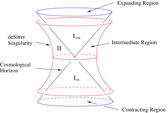
Figure 16: The space–time global structure. We shall see that the geometry develops a time–like singularity in region $II$ interpreted as a deSitter negative tension brane at the boundary of space–time. This geometry describes a transition from a contracting to an expanding cosmological phase. Clearly, with this space–time global structure the standard cosmological horizon problem, associated with the conventional big–bang space–like singularity, does not arise.

The existence of an intermediate region with a generic metric of the form (46) implies that any singularity that may develop in this region is time–like, with a deSitter worldvolume. As we shall see bellow, this fact introduces the possibility of having a brane–like interpretation of the singularity. Moreover, the existence of this region demands generically a field theory effective potential whose form is highly restrictive due to the unnatural (fine–tuned) boundary conditions at the horizon. As we shall also see, string effective supergravity theories provide a Liouville–Toda like potential which naturally respects the boundary conditions at the horizon.

4.3.1 Embedding in String Theory

Let us now consider a particular case of the construction of the previous section which can be embedded in Type IIA string theory (or M–theory). We consider a background with a non–trivial $RR$ 9–form potential. The corresponding ten–dimensional Type II effective theory is given by the massive supergravity theory, and in this case the relevant action is

$$S=\frac{1}{(2\pi)^{7}\,\hat{l}_{s}^{\,8}}\,\left[\int d^{10}x\,\sqrt{-g}\,e^{-2\phi}\left(R+4\left(\nabla\phi\right)^{2}\right)-\frac{1}{2}\int F\wedge\widetilde{F}\,\right]\ ,$$

where $F$ is a $RR$ 10–form field strength and $\widetilde{F}=\star F$ is related to the cosmological constant. As mentioned before, we are considering a particular case for simplicity, but the analysis can be extended to any dimensionality and degree of the form potential [22]. Also, we consider a solution of massive SUGRA to make contact with the $O8$–plane interpretation of the previous sections. A family of solutions, parameterized by an arbitrary constant $\hat{g}_{s}$, can be constructed by considering the following ansatz

$$\begin{array}[]{c}\displaystyle{{\cal E}^{2}\,ds^{2}=\Lambda^{-1}\,ds_{4}^{\,2}+\Lambda^{-1/2}\,ds^{2}(\hbox{\mybb T}^{6})}\ ,\phantom{\framebox{\rule[-8.5359pt]{0.0pt}{0.0pt}}}\\ \displaystyle{e^{\phi}=\hat{g}_{s}\,\Lambda^{-5/4}\ ,\ \ \ \ \ \ \ \ \ \star F={\cal E}}\ ,\end{array}$$ (47)

where the line element $ds_{4}$ is that of the previous section and we conveniently define the scalar field $\psi$ by

$$\Lambda=e^{\,2\psi/7}\ .$$

The constants $\cal E$ and $\hat{g}_{s}$ define the electric field and the string coupling at the horizon, respectively. It is now a mater of computation to show that the equations of motion for the effective four–dimensional theory can be derived from the action (42) with

$$V=\frac{1}{2}\,e^{-\psi}\ ,\ \ \ \ \ \ \ \ \ \ \beta=\frac{1}{7}\ .$$ (48)

Let us start by considering the expanding region ${\mathrm{I}}_{out}$. Solving in powers of the dimensionless coordinate $t$ around the cosmological horizon, a straightforward calculation gives the first terms in this expansion

$$\begin{array}[]{c}\displaystyle{a_{\mathrm{I}}(t)=t\,\left(1+\frac{e^{-\psi_{0}}}{18}\,t^{2}+\cdots\right)}\ ,\phantom{\framebox{\rule[-11.38092pt]{0.0pt}{0.0pt}}}\\ \displaystyle{\psi(t)=\psi_{0}+\frac{7e^{-\psi_{0}}}{4}\,t^{2}+\cdots}\ .\end{array}$$ (49)

At late times the universe becomes curvature dominated and the solution has the asymptotic behavior

$$a(t)=\sqrt{\frac{7}{6}}\,t\ ,\ \ \ \ \ \ \ \ \ \ \psi(t)=\log\left(\,\frac{7}{8}\,t^{2}\,\right)\ ,$$ (50)

so that the scalar field is rolling down the potential. The solution in the contracting region ${\mathrm{I}}_{in}$ is the time reversal of the solution in the expanding region.

Figure 17: Behavior of the scalar field along the potential in regions I and II. Starting from the horizon, where $\psi=\psi_{0}$, the scalar field rolls down the potential along region ${\mathrm{I}}_{out}$ and has the time reversed behavior in region ${\mathrm{I}}_{in}$. In region II the equations of motion are equivalent to those with an inverted potential potential, and therefore the field roles to $-\infty$ at the singularity.

Next consider the intermediate region ${\mathrm{I}I}$. The form of the solution near the horizon can be obtained simply from the analytic continuation

$$\begin{array}[]{c}\displaystyle{a_{\mathrm{I}I}(x)=x\,\left(1-\frac{1}{18}\,e^{-\psi_{0}}\,x^{2}+\cdots\right)}\ ,\phantom{\framebox{\rule[-11.38092pt]{0.0pt}{0.0pt}}}\\ \displaystyle{\psi_{\mathrm{I}I}(x)=\psi_{0}-\frac{7}{4}\,e^{-\psi_{0}}\,x^{2}+\cdots}\ .\end{array}$$ (51)

One can then integrate the differential equations away from the horizon, to see that the geometry develops a time–like singularity, where the scale factor and the scalar field have the behavior

$$\begin{array}[]{c}\displaystyle{a_{\mathrm{I}I}\left(x\right)=a_{s}\left(x_{s}-x\right)^{1/7}}\ ,\phantom{\framebox{\rule[-8.5359pt]{0.0pt}{0.0pt}}}\\ \displaystyle{\psi_{\mathrm{I}I}\left(x\right)=2\,\log{\left(\frac{7}{4}\,\left(x_{s}-x\right)\right)}}\ .\end{array}$$ (52)

The dimensionless constants $a_{s}$ and $x_{s}$ can be determined numerically, and are fixed by the boundary conditions imposed at the horizon. The behavior of the scalar field along the potential is represented schematically in figure 17. The CP diagram for this geometry is represented in figure 18, where it is compared with the standard diagram for an open cosmology. Let us remark that the global structure of this model is related to the earlier work of Hawking and Turok [102], where the top half of diagram 18(a) is glued to an Euclidean gravitational instanton.

Figure 18: CP diagrams for open Universe cosmologies. In both diagrams each point represents a two–sphere and $\chi=0$ is a coordinate singularity. The standard diagram, with a space–like singularity, is presented for comparison with the orientifold cosmology diagram.

Before we investigate the geometry near the singularity, let us comment on the issue of cosmological particle production for this geometry. Generically, from the existence of a horizon, one expects Hawking thermal radiation. In fact, in the two–dimensional toy model associated to the shifted–boost orbifold, we showed that, starting from the asymptotic vacuum in the contracting region, an observer in the far future sees a thermal spectrum. To extend this result to a four–dimensional cosmological solution one just needs to compute the surface gravity of the cosmological horizon with respect to the appropriate Killing vector field. The natural Killing vector fields to use are the generators of the $SO(1,3)$ isometries of $H_{3}$. With this in mind, one arrives at the general result

$$T=\frac{{\mathcal{E}}}{2\pi\,a(\tau)}\ .$$ (53)

This is expected for radiation in a three–dimensional cosmology, since, from Boltzmann law $\rho\sim T^{4}$, we obtain $\rho\sim 1/a^{4}(\tau)$, which follows from the radiation equation of state $\rho=3\,p$.

Like in the two–dimensional toy model of the previous section, to make sense of this geometry it is fundamental to understand the naked singularity. From the behavior of the scalar field at the singularity $(\psi\rightarrow-\infty)$ and at the horizon $(\psi=\psi_{0})$, and from the fact that the scalar field is a growing function as one moves from the singularity to the horizon, it is natural to use $\Lambda$ as a radial variable instead of $x$. At the singularity we have $\Lambda=0$ and at the light–cone $\Lambda=\Lambda_{0}\equiv e^{2\psi_{0}/7}$. Then, near the singularity, in the limit $\Lambda\ll\Lambda_{0}$, we obtain the following ten–dimensional metric

$${\cal E}^{2}ds^{2}=\Lambda^{-1/2}\left(\,\mu\,ds^{2}(dS_{3})+ds^{2}\left(\hbox{\mybb T}^{6}\right)\right)+\Lambda^{1/2}d\Lambda^{2}\ .$$

The dilaton field and the cosmological constant are still given by (47) and the constant $\mu$ can be determined from $a_{s}$ in the expansion (52). This geometry looks very similar to the $O8$–plane geometry of section 4.1, with the important difference that the orientifold has worldvolume $dS_{3}\times\hbox{\mybb T}^{6}$, with deSitter radius $\sqrt{\mu}$. In the limit $\Lambda\rightarrow 0$ the curvature of the induced metric on the orientifold worldvolume vanishes, so that locally the orientifold looks flat. This is simply a higher dimensional generalization of the $O8/\overline{O}8$ system, since now one has a single $O8$–plane with spatial worldvolume $S^{2}\times T^{6}$. Antipodal points on the sphere will have opposite charges, and therefore the near singularity geometry is locally BPS but breaks SUSY globally. These arguments are purely based on the supergravity description of the system and should be taken only as such. In fact, while there is a perturbative string theory definition of the $O8/\overline{O}8$ system at zero coupling, such definition does not exist for this curved $O8$–plane. If the locally flat description of the $O8$–plane is valid in string theory, one can quantize the charge as before, with the result

$$2\pi\hat{l}_{s}\,{\cal E}=8\,\hat{g}_{s}\ .$$

Naively the solution just described is parameterized by $\hat{g}_{s}$, ${\cal E}$ and the position of the horizon $\Lambda_{0}$. However, we can set $\Lambda_{0}=1$ using the rescaling of the coordinates $\Lambda\to c\Lambda$ and $\hbox{\mybb T}^{6}\to c\,\hbox{\mybb T}^{6}$, which leaves the form of the solution invariant, if we also redefine $\hat{g}_{s}\to c^{-1/4}\,\hat{g}_{s}\,$, ${\cal E}\to c^{5/4}\,{\cal E}$. Therefore, after imposing the quantization of the orientifold charge, the solution is parametrized only by the string coupling. The situation is analogous to the $O8/\overline{O}8$ system, where the geometry is fixed by a single constant of motion which is determined only, after charge quantization, by the string coupling.

4.3.2 Cosmological acceleration

When the scale factor vanishes, according to the behavior (49), one has a non–singular cosmological horizon. Naturally, to evade the singularity theorems briefly discussed in the introduction, it must be that the strong energy condition is violated. In fact, the boundary condition imposed on the scalar field at the horizon was $\dot{\psi}=0$, and therefore the kinetic energy at the horizon vanishes. At this point, all the field’s energy is in the form of the potential energy $V(\psi_{0})$, which acts as a positive cosmological constant. Hence, in this region the field does not obey the strong energy condition, explaining why in both regions I there are no singularities. Moreover, the power expansion (49) shows that the scale factor starts with an acceleration, as noted in [19]. The fact that a period of transient acceleration is quite generic, whenever the kinetic energy vanishes and the potential is positive, was shown in the context of String/M–theory compactifications in [103].

The above acceleration occurs near the cosmological horizon. Another important question, related to the current observed acceleration of the universe, is whether this geometry exhibits a late time acceleration. This problem has been considered recently by many people in the context of time–dependent string compactifications [104]–[115]. Clearly, this can be answered by analyzing the convergence to the asymptotic solution (50). This is a well posed problem in dynamical systems and was investigated in great detail by Halliwell [116] for the cases of open ($k=-1$), flat ($k=0$) and closed ($k=1$) four–dimensional cosmologies with an exponential potential of the type here considered. Let us review here Halliwell’s results. Start with a scalar field with canonically normalized kinetic energy and consider a family of potentials, parametrized by a constant $a>0$, of the form

$$V(\psi)=\Lambda\,e^{-a\psi}\,,\ \ \ \ \ \ \ \ \ \ \ \ \ \ \ \ \ \ \ \ (\Lambda>0)\,,$$

together with the FRW geometry

$$-N^{2}\left(t\right)\,dt^{2}+e^{2A\left(t\right)}\,ds^{2}\left(\mathcal{M}_{k}\right),$$

where we introduce the lapse function $N\left(t\right)$ to allow for a more general time coordinate, and where $\mathcal{M}_{k}$ is $\mathbb{M}^{3}$, $S^{3}$ or $H^{3}$ depending on whether $k=0,1,-1$. The Friedman equation reads

$$\frac{\dot{A}^{2}}{N^{2}}+k\,e^{-2A}=\frac{1}{12}\,\frac{\dot{\psi}^{2}}{N^{2}}\,+\frac{1}{6}\,V\left(\psi\right),$$

and the usual equations of motion for $A$ and $\psi$ are

$$\frac{1}{N}\,\frac{d}{dt}\left(\frac{\dot{A}}{N}\right)-k\,e^{-2A}+\frac{1}{4}\,\frac{\dot{\psi}^{2}}{N^{2}}=0\,,$$

$$\frac{1}{N}\,\frac{d}{dt}\left(\frac{\dot{\psi}}{N}\right)+3N^{-2}\dot{A}\,\dot{\psi}+V^{\prime}\left(\psi\right)=0\,.$$

We shall choose a time coordinate $t$ such that $N^{2}=V^{-1}$. It is then easy to check that the Friedman equation becomes

$$\dot{A}^{2}-\frac{1}{12}\,\dot{\psi}^{2}=\frac{1}{6}-\frac{k}{\Lambda}\,e^{a\psi-2A}\,.$$

Therefore the hyperbola $\dot{A}^{2}=\frac{1}{12}\,\dot{\psi}^{2}+\frac{1}{6}$ divides the regions where $k$ is positive or negative. Moreover, the equations of motion reduce to the following dynamical system

$$\ddot{A}=\frac{1}{6}-\frac{1}{6}\,\dot{\psi}^{2}-\dot{A}^{2}+\frac{a}{2}\,\dot{A}\,\dot{\psi}\,,$$

$$\ddot{\psi}=\frac{a}{2}\,\dot{\psi}^{2}-3\dot{A}\,\dot{\psi}+a\,,$$

which has fixed points in the $\dot{\psi}\dot{A}$–plane (neglecting the ones obtained by $t\rightarrow-t$, which correspond to a contracting universe)

$$P_{1} = \left(\frac{a\sqrt{2}}{\sqrt{3-a^{2}}}\,,\frac{1}{\sqrt{2(3-a^{2})}}\right)\,,$$ (54)

$$P_{2} = \left(1,\,\frac{a}{2}\,\right)\,.$$

Note that $P_{1}$ is always on the $k=0$ parabola.

To check if the corresponding cosmological solution is accelerating, we must check the positivity of the second derivative of the scale factor with respect to proper time

$$\left(\frac{1}{N}\frac{d}{dt}\right)^{2}e^{A}>0\,.$$

Using the above equations, it is easy to check that this condition is equivalent to [26]

$$\dot{\psi}^{2}<1\,.$$

Now we can analyze the various trajectories in the $\dot{\psi}\dot{A}$–plane, and check whether they correspond to an accelerating universe. We first note that the attractor solution is $P_{1}$ for $0<a<1$ and is $P_{2}$ otherwise. Moreover, for $a>\sqrt{3}$ the point $P_{1}$ no longer exists. Generically flux compactifications have $a>\sqrt{3}$. This includes the string compactification considered in the previous section where $a=\sqrt{7}$. On the other hand, in hyperbolic compactifications [104], where the field $\psi$ is related to the size of an internal compactification hyperbolic manifold of dimension $n\geq 2$, one has

$$1<a=\sqrt{\frac{n+2}{n}}<\sqrt{3}\,.$$

Therefore, in both cases, the attractor solution has $k=-1$  and is given by $P_{2}$.

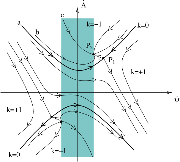
Figure 19: Trajectories in the $\dot{\psi}\dot{A}$–plane for $1<a<\sqrt{4/3}$. When $\sqrt{4/3}<a<\sqrt{3}$ the diagram is similar but the trajectories spiral around the stable attractors. These are the two regimes associated with hyperbolic compactifications. Inside the shaded region the universe is accelerating, whereas outside it decelerates.

Let us first consider the fixed point $P_{1}$, by concentrating, for the moment, on a flat universe with $k=0$. The class of solutions for a flat universe and arbitrary constant $a$ were found explicitly in [115]. For $0<a<\sqrt{3}$, the point $P_{1}$ is always an attractor, if we restrict to the $k=0$ hyperbola. We must then distinguish two cases. For $a<1$, and therefore not for hyperbolic or flux compactifications, the fixed point has $\dot{\psi}^{2}<1$. Hence, the asymptotic solution is accelerating. The particular case with $a=1$ has a solution which accelerates and a solution which decelerates, depending if one starts from $\dot{\psi}=\mp\infty$. In particular, the accelerating solution does not have a future event horizon [115]. For $1<a<\sqrt{3}$, which includes hyperbolic compactifications, the asymptotic solution is always decelerating (figure 19). For example, let us consider, following [104], the trajectory (a) in figure 19, starting with large negative $\dot{\psi}$ (the field rolling up the potential). Then, as $\dot{\psi}^{2}$ becomes less then $1$, we enter into a period of transient acceleration, followed again by a period of deceleration. Finally, for $a>\sqrt{3}$, the $k=0$ trajectory (a) of figure 20, associated to flux compactifications, has a runaway behavior, always with a period of transient acceleration.

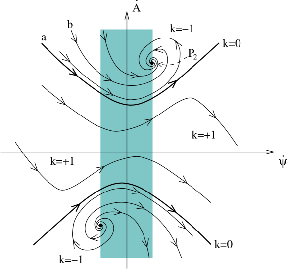
Figure 20: Trajectories in the $\dot{\psi}\dot{A}$–plane for $a>\sqrt{3}$, corresponding to flux compactifications. The late time behavior of the acceleration is always oscillatory.

Let us move to the case of $k=-1$, with $a>1$, where there is always an attractor at $P_{2}$. Note that $P_{2}$ is on the boundary of the region $\dot{\psi}^{2}<1$ of acceleration, because at late times curvature dominates and one has linear expansion. Consequently, these geometries do not have a future event horizon. The behavior of the trajectories converging to $P_{1}$ changes at $a=\sqrt{4/3}$ (see [116] for details). For $a<\sqrt{4/3}$ the trajectories are as in figure 19, whereas for $a>\sqrt{4/3}$ the trajectories spiral to $P_{2}$, like in figure 20. Whenever $a<\sqrt{4/3}$, we can arrange initial conditions to have a period of transient acceleration similar to the $k=0$ case, as in the trajectory (b) in figure 19. Other initial conditions will give a cosmology with a late time acceleration, as for the trajectory (c) in the same figure. When $a>\sqrt{4/3}$ (so, in particular, for all flux compactifications and for hyperbolic compactifications with $n<6$), independently of initial conditions, we have a cyclic behavior, with the acceleration oscillating around zero, with decreasing magnitude.

To summarize, for open cosmologies, both compactifications can give at late times periods of positive acceleration. This result is in contrast with the case of flat universes, where a positive acceleration is always transient for both type of compactifications.

5 Conclusion

In these lectures we have extensively discussed the physics of time–dependent orbifolds of string theory, focusing on the key examples of orbifolds of three–dimensional Minkowski space, together with their implications for the study of the cosmological singularity. Although the free propagation of particles is well understood, the physics of interactions presents new challenges which are intimately tied with the physics of quantum gravity at trans–Planckian energies. At first, the problem seems insurmountable, of the same order of complexity as the analysis of black–hole singularities. On the other hand, as we have discussed in the section of eikonal resummation, there are hints that one can have a better control over these theories, due to their orbifold structure and to some partial facts known about gravity at high energies in flat space–time. Certainly these models are a laboratory where we can try to push our knowledge of quantum gravity to its limits. Such an example is the series of string dualities that led us to conjecture a remarkably simple quantization condition for the gravitational constant in the presence of closed time–like curves. This condition is related to quantization of charge, and should rely only on basic properties of quantum gravity, together with the requirement of unitarity of the orbifold theory. Therefore, even though we are probing physics at trans–Planckian energies, we are in a more controlled situation than with black–holes, and more conclusive statements can be made.

Acknowledgments: We are grateful to Costas Kounnas for many discussions and collaboration on some of the material here presented. We would also like to thank Carlos Herdeiro, Costas Bachas, Fernando Quevedo, Frank Ferrari, Gianmassimo Tasinato, Ivonne Zavala, Joe Polchinski, Paul Steinhardt, Neil Turok, Paul Townsend, Rodolfo Russo and Pedro Vieira for discussions and correspondence. We are both grateful to the organizers of the RTN Winter School in Torino for a great meeting and for their kind hospitality. M.S.C. thanks Amsterdam University and L.C. thanks Oporto University for hospitality during the course of these work. We are also grateful to LPTENS and DAMTP for their hospitality. L.C. is supported by a Marie Curie Fellowship under the European Commission’s Improving Human Potential programme (HPMF–CT–2002–02016). This work is partially funded by CERN under contract POCTI/FNU/49507/2002–FEDER and by FCT under contract POCTI/FNU/38004/2001–FEDER.

References

- [1] S. W. Hawking and G. F. R. Ellis, The large scale structure of space–time, Cambridge Monographs on Mathematical Physics, Cambridge University Press (1973).
- [2] M. B. Green, J. H. Schwarz and E. Witten, Superstring Theory. Vol. 1 and 2, Cambridge Monographs on Mathematical Physics, Cambridge University Press (1987).
- [3] J. Polchinski, String Theory. Vol. 1 and 2, Cambridge Monographs on Mathematical Physics, Cambridge University Press (1998).
- [4] A. H. Guth, The Inflationary Universe: A Possible Solution To The Horizon And Flatness Problems, Phys. Rev. D 23 (1981) 347.
- [5] J. B. Hartle and S. W. Hawking, Wave Function Of The Universe, Phys. Rev. D 28 (1983) 2960.
- [6] G. Veneziano, String Cosmology: The Pre–Big Bang Scenario, Les Houches 1999 – The primordial universe, 581–628, hep-th/0002094.
- [7] J. Khoury, B. A. Ovrut, P. J. Steinhardt and N. Turok, The ekpyrotic universe: Colliding branes and the origin of the hot big bang, Phys. Rev. D 64 (2001) 123522, hep-th/0103239; Density perturbations in the ekpyrotic scenario, Phys. Rev. D 66 (2002) 046005, hep-th/0109050.
- [8] P. J. Steinhardt and N. Turok, Cosmic evolution in a cyclic universe, Phys. Rev. D 65 (2002) 126003, hep-th/0111098.
-
[9]
J. Khoury, B. A. Ovrut, N. Seiberg, P. J. Steinhardt and N. Turok,
From big crunch to big bang,
Phys. Rev. D 65 (2002) 086007,
hep-th/0108187.
N. Seiberg, From big crunch to big bang – is it possible?, hep-th/0201039. -
[10]
A. J. Tolley and N. Turok,
Quantum fields in a big crunch / big bang spacetime,
Phys. Rev. D 66 (2002) 106005,
hep-th/0204091.
C. Gordon and N. Turok, Cosmological perturbations through a general relativistic bounce, Phys. Rev. D 67 (2003) 123508, hep-th/0206138.
A. J. Tolley, N. Turok and P. J. Steinhardt, Cosmological perturbations in a big crunch / big bang space–time, hep-th/0306109. - [11] G. T. Horowitz and A. R. Steif, Singular String Solutions With Nonsingular Initial Data, Phys. Lett. B 258 (1991) 91.
- [12] G. T. Horowitz and J. Polchinski, Instability of spacelike and null orbifold singularities, Phys. Rev. D 66 (2002) 103512, hep-th/0206228.
- [13] A. Lawrence, On the instability of 3D null singularities, JHEP 0211 (2002) 019, hep-th/0205288.
- [14] L. Cornalba and M. S. Costa, On the classical stability of orientifold cosmologies, Class. Quant. Grav. 20 (2003) 3647, hep-th/0302137.
- [15] H. Liu, G. Moore and N. Seiberg, Strings in a time–dependent orbifold, JHEP 0206 (2002) 045, hep-th/0204168.
- [16] H. Liu, G. Moore and N. Seiberg, Strings in time–dependent orbifolds, JHEP 0210 (2002) 031, hep-th/0206182.
- [17] M. Berkooz, B. Craps, D. Kutasov and G. Rajesh, Comments on cosmological singularities in string theory, JHEP 0303 (2003) 031, hep-th/0212215.
- [18] L. Cornalba and M. S. Costa, to appear.
- [19] L. Cornalba and M. S. Costa, A New Cosmological Scenario in String Theory, Phys. Rev. D 66 (2002) 066001, hep-th/0203031.
- [20] N. A. Nekrasov, Milne universe, tachyons, and quantum group, Surveys High Energ. Phys. 17 (2002) 115, hep-th/0203112.
- [21] B. Pioline and M. Berkooz, Strings in an electric field, and the Milne universe, hep-th/0307280.
- [22] L. Cornalba, M. S. Costa and C. Kounnas, A resolution of the cosmological singularity with orientifolds, Nucl. Phys. B 637 (2002) 378, hep-th/0204261.
- [23] C. Kounnas and D. Lust, Cosmological string backgrounds from gauged WZW models, Phys. Lett. B 289 (1992) 56, hep-th/9205046.
- [24] C. Grojean, F. Quevedo, G. Tasinato and I. Zavala, Branes on charged dilatonic backgrounds: Self–tuning, Lorentz violations and cosmology, JHEP 0108 (2001) 005, hep-th/0106120.
- [25] C. P. Burgess, F. Quevedo, S. J. Rey, G. Tasinato and I. Zavala, Cosmological spacetimes from negative tension brane backgrounds, JHEP 0210 (2002) 028, hep-th/0207104.
- [26] P. G. Vieira, Late-time cosmic dynamics from M-theory, Class. Quant. Grav. 21 (2004) 2421, hep-th/0311173.
- [27] V. Balasubramanian, S. F. Hassan, E. Keski–Vakkuri and A. Naqvi, A space–time orbifold: A toy model for a cosmological singularity, Phys. Rev. D 67 (2003) 026003, hep-th/0202187.
- [28] J. Simon, The geometry of null rotation identifications, JHEP 0206 (2002) 001, hep-th/0203201.
- [29] S. Elitzur, A. Giveon, D. Kutasov and E. Rabinovici, From big bang to big crunch and beyond, JHEP 0206 (2002) 017, hep-th/0204189.
- [30] B. Craps, D. Kutasov and G. Rajesh, String propagation in the presence of cosmological singularities, JHEP 0206 (2002) 053, hep-th/0205101.
- [31] E. J. Martinec and W. McElgin, Exciting AdS orbifolds, JHEP 0210 (2002) 050, hep-th/0206175.
- [32] M. Fabinger and J. McGreevy, On smooth time–dependent orbifolds and null singularities, JHEP 0306 (2003) 042, hep-th/0206196.
- [33] A. Buchel, P. Langfelder and J. Walcher, On time–dependent backgrounds in supergravity and string theory, Phys. Rev. D 67 (2003) 024011, hep-th/0207214.
- [34] S. Hemming, E. Keski–Vakkuri and P. Kraus, Strings in the extended BTZ spacetime, JHEP 0210 (2002) 006, hep-th/0208003.
- [35] A. Hashimoto and S. Sethi, Holography and string dynamics in time–dependent backgrounds, Phys. Rev. Lett. 89 (2002) 261601, hep-th/0208126.
- [36] J. Simon, Null orbifolds in AdS, time dependence and holography, JHEP 0210 (2002) 036, hep-th/0208165.
- [37] M. Alishahiha and S. Parvizi, Branes in time–dependent backgrounds and AdS/CFT correspondence, JHEP 0210 (2002) 047, hep-th/0208187.
- [38] E. Dudas, J. Mourad and C. Timirgaziu, Time and space dependent backgrounds from nonsupersymmetric strings, Nucl. Phys. B 660 (2003) 3, hep-th/0209176.
- [39] Y. Satoh and J. Troost, Massless BTZ black holes in minisuperspace, JHEP 0211 (2002) 042, hep-th/0209195.
- [40] L. Dolan and C. R. Nappi, Noncommutativity in a time–dependent background, Phys. Lett. B 551 (2003) 369, hep-th/0210030.
- [41] R. G. Cai, J. X. Lu and N. Ohta, NCOS and D-branes in time–dependent backgrounds, Phys. Lett. B 551 (2003) 178, hep-th/0210206.
-
[42]
C. Bachas and C. Hull,
Null brane intersections,
JHEP 0212 (2002) 035,
hep-th/0210269. - [43] R. C. Myers and D. J. Winters, From D– anti–D pairs to branes in motion, JHEP 0212 (2002) 061, hep-th/0211042.
- [44] K. Okuyama, D–branes on the null–brane, JHEP 0302 (2003) 043, hep-th/0211218.
- [45] G. Papadopoulos, J. G. Russo and A. A. Tseytlin, Solvable model of strings in a time–dependent plane–wave background, Class. Quant. Grav. 20 (2003) 969, hep-th/0211289.
- [46] T. Friedmann and H. Verlinde, Schwinger meets Kaluza–Klein, hep-th/0212163.
-
[47]
M. Fabinger and S. Hellerman,
Stringy resolutions of null singularities,
hep-th/0212223. - [48] S. Elitzur, A. Giveon and E. Rabinovici, Removing singularities, JHEP 0301 (2003) 017, hep-th/0212242.
- [49] P. Kraus, H. Ooguri and S. Shenker, Inside the horizon with AdS/CFT, Phys. Rev. D 67 (2003) 124022, hep-th/0212277.
- [50] B. Durin and B. Pioline, Open strings in relativistic ion traps, JHEP 0305 (2003) 035, hep-th/0302159.
- [51] J. R. David, Plane waves with weak singularities, hep-th/0303013.
- [52] R. Biswas, E. Keski-Vakkuri, R. G. Leigh, S. Nowling and E. Sharpe, The taming of closed time–like curves, hep-th/0304241.
- [53] J. G. Russo, Cosmological string models from Milne spaces and orbifold, hep-th/0305032.
- [54] A. Giveon, E. Rabinovici and A. Sever, Strings in singular time–dependent backgrounds, Fortsch. Phys. 51 (2003) 805, hep-th/0305137.
- [55] L. Fidkowski, V. Hubeny, M. Kleban and S. Shenker, The black hole singularity in AdS/CFT, hep-th/0306170.
- [56] B. Craps and B. A. Ovrut, Global fluctuation spectra in big crunch / big bang string vacua, hep-th/0308057.
- [57] E. Dudas, J. Mourad and C. Timirgaziu, On cosmologically induced hierarchies in string theory, hep-th/0309057.
- [58] P. Fre, V. Gili, F. Gargiulo, A. Sorin, K. Rulik and M. Trigiante, Cosmological backgrounds of superstring theory and Solvable Algebras: Oxidation and Branes, hep-th/0309237.
- [59] C. P. Bachas and M. R. Gaberdiel, World–sheet duality for D–branes with travelling waves, hep-th/0310017.
- [60] L. J. Dixon, J. A. Harvey, C. Vafa and E. Witten, Strings On Orbifolds, Nucl. Phys. B 261 (1985) 678; Strings On Orbifolds. 2, Nucl. Phys. B 274 (1986) 285.
- [61] S. Kachru and E. Silverstein, 4d conformal theories and strings on orbifolds, Phys. Rev. Lett. 80 (1998) 4855, hep-th/9802183.
- [62] A. E. Lawrence, N. Nekrasov and C. Vafa, On conformal field theories in four dimensions, Nucl. Phys. B 533 (1998) 199, hep-th/9803015.
- [63] J. Figueroa–O’Farrill and J. Simon, Generalized supersymmetric fluxbranes, JHEP 0112 (2001) 011, hep-th/0110170.
- [64] G. W. Moore, Finite In All Directions, hep-th/9305139.
- [65] S. W. Kim and K. P. Thorne, Do Vacuum Fluctuations Prevent The Creation Of Closed Timelike Curves?, Phys. Rev. D 43 (1991) 3929.
- [66] J. C. Breckenridge, R. C. Myers, A. W. Peet and C. Vafa, D-branes and spinning black holes, Phys. Lett. B 391 (1997) 93, hep-th/9602065.
- [67] G. W. Gibbons and C. A. R. Herdeiro, Supersymmetric rotating black holes and causality violation, Class. Quant. Grav. 16 (1999) 3619, hep-th/9906098; C. A. R. Herdeiro, Special properties of five dimensional BPS rotating black holes, Nucl. Phys. B 582 (2000) 363, hep-th/0003063.
- [68] M. Banados, M. Henneaux, C. Teitelboim and J. Zanelli, Geometry of the (2+1) black hole, Phys. Rev. D 48 (1993) 1506, gr-qc/9302012.
- [69] M. Simpson and R. Penrose, Internal Instability in a Reissner–Nordstrom Black Hole, Int. Journ. Theor. Physics 7 (1973) 183.
- [70] S. Chandrasekhar and J. B. Hartle, On Crossing the Cauchy Horizon of a Reissner–Nordstrom Black–Hole, Proc. R. Soc. Lond. A 384 (1982) 301.
- [71] C. P. Burgess, P. Martineau, F. Quevedo, G. Tasinato and I. Zavala C., Instabilities and particle production in S–brane geometries, hep-th/0301122.
- [72] L. Randall and R. Sundrum, A large mass hierarchy from a small extra dimension, Phys. Rev. Lett. 83 (1990) 3370, hep-ph/9905221; An alternative to compactification, Phys. Rev. Lett. 83 (1990) 4690, hep-th/9906064.
- [73] P. C. Aichelburg and R. U. Sexl, On The Gravitational Field Of A Massless Particle, Gen. Rel. Grav. 2 (1971) 303.
- [74] P. D. D’Eath and P. N. Payne, Gravitational Radiation In High Speed Black Hole Collisions. 1. Perturbation Treatment Of The Axisymmetric Speed Of Light Collision, Phys. Rev. D 46 (1992) 658.
- [75] P. J. Steinhardt, A. J. Tolley and N. Turok, unpublished.
- [76] D. Louis-Martinez and G. Kunstatter, On Birckhoff’s theorem in 2–D dilaton gravity, Phys. Rev. D 49 (1994) 5227.
- [77] D. Grumiller, W. Kummer and D. V. Vassilevich, Dilaton gravity in two dimensions, Phys. Rept. 369 (2002) 327, hep-th/0204253.
- [78] C. G. Callan, S. B. Giddings, J. A. Harvey and A. Strominger, Evanescent Black Holes, Phys. Rev. D 45 (1992) 1005, hep-th/9111056.
- [79] J. R. Gott, Closed Timelike Curves Produced By Pairs Of Moving Cosmic Strings: Exact Solutions, Phys. Rev. Lett. 66 (1991) 1126.
- [80] S. Deser, R. Jackiw and G. ’t Hooft, Physical cosmic strings do not generate closed timelike curves, Phys. Rev. Lett. 68 (1992) 267.
- [81] D. N. Kabat, Conditions For The Existence Of Closed Timelike Curves In (2+1) Gravity, Phys. Rev. D 46 (1992) 2720.
- [82] M. P. Headrick and J. R. Gott, (2+1)–Dimensional Space–Times Containing Closed Timelike Curves, Phys. Rev. D 50 (1994) 7244.
- [83] H. Cheng and T. T. Wu, High–Energy Elastic Scattering In Quantum Electrodynamics, Phys. Rev. Lett. 22 (1969) 666.
- [84] H. D. Abarbanel and C. Itzykson, Relativistic Eikonal Expansion, Phys. Rev. Lett. 23 (1969) 53.
- [85] M. Levy and J. Sucher, Eikonal Approximation In Quantum Field Theory, Phys. Rev. 186 (1969) 1656.
- [86] I. J. Muzinich and M. Soldate, High–Energy Unitarity Of Gravitation And Strings, Phys. Rev. D 37 (1988) 359.
- [87] D. Amati, M. Ciafaloni and G. Veneziano, Superstring Collisions At Planckian Energies, Phys. Lett. B 197 (1987) 81; Classical And Quantum Gravity Effects From Planckian Energy Superstring Collisions, Int. J. Mod. Phys. A 3 (1988) 1615; Higher Order Gravitational Deflection And Soft Bremsstrahlung In Planckian Energy Superstring Collisions, Nucl. Phys. B 347 (1990) 550.
- [88] G. ’t Hooft, Graviton Dominance In Ultrahigh–Energy Scattering, Phys. Lett. B 198 (1987) 61.
- [89] S. Deser, J. G. McCarthy and A. R. Steif, Ultraplanck Scattering In Gravity Theories, Nucl. Phys. B 412 (1994) 305, hep-th/9307092.
- [90] J. M. Maldacena, H. Ooguri and J. Son, Strings in AdS(3) and the SL(2,R) WZW model. II: Euclidean black hole, J. Math. Phys. 42, 2961 (2001, hep-th/0005183.
- [91] C. Bachas, D–brane dynamics, Phys. Lett. B 374 (1996) 37, hep-th/9511043.
-
[92]
J. G. Russo and A. A. Tseytlin,
Constant magnetic field in closed string theory:
An Exactly solvable model,
Nucl. Phys. B 448 (1995) 293, hep-th/9411099;
Magnetic flux tube models in superstring theory,
Nucl. Phys. B 461 (1996) 131, hep-th/9508068;
A. A. Tseytlin, Closed superstrings in magnetic flux tube background, Nucl. Phys. Proc. Suppl. 49 (1996) 338, hep-th/9510041. - [93] L. J. Romans, Massive N=2a Supergravity In Ten–Dimensions, Phys. Lett. B 169 (1986) 374.
- [94] E. Bergshoeff, M. de Roo, M. B. Green, G. Papadopoulos and P. K. Townsend, Duality of Type II 7–branes and 8–branes, Nucl. Phys. B 470 (1996) 113, hep-th/9601150.
- [95] J. Polchinski and E. Witten, Evidence for Heterotic – Type I String Duality, Nucl. Phys. B 460 (1996) 525, hep-th/9510169.
- [96] J. Polchinski, Lectures on D–branes, Fields, strings and duality, 293–356, Boulder (1996), hep-th/9611050.
- [97] C. Angelantonj and A. Sagnotti, Open strings, Phys. Rept. 371 (2002) 1, Erratum–ibid. 376 (2003) 339, hep-th/0204089.
- [98] S. W. Hawking, The Chronology protection conjecture, Phys. Rev. D 46 (1992) 603.
- [99] I. Antoniadis, E. Dudas and A. Sagnotti, Supersymmetry breaking, open strings and M–theory, Nucl. Phys. B 544 (1999) 469, hep-th/9807011.
- [100] S. Kachru, J. Kumar and E. Silverstein, Orientifolds, RG flows, and closed string tachyons, Class. Quant. Grav. 17 (2000) 1139, hep-th/9907038.
- [101] A. Vilenkin, Gravitational Field Of Vacuum Domain Walls And Strings, Phys. Rev. D 23 (1981) 852.
- [102] S. W. Hawking and N. Turok, Open inflation without false vacua, Phys. Lett. B 425 (1998) 25, hep-th/9802030.
- [103] R. Emparan and J. Garriga, A note on accelerating cosmologies from compactifications and S–branes, JHEP 0305 (2003) 028, hep-th/0304124.
- [104] P. K. Townsend and M. N. Wohlfarth, Accelerating cosmologies from compactification, Phys. Rev. Lett. 91 (2003) 061302, hep-th/0303097.
- [105] N. Ohta, Accelerating cosmologies from S–branes, Phys. Rev. Lett. 91 (2003) 061303, hep-th/0303238.
- [106] S. Roy, Accelerating cosmologies from M/string theory compactifications, Phys. Lett. B 567 (2003) 322, hep-th/0304084.
- [107] M. N. Wohlfarth, Accelerating cosmologies and a phase transition in M–theory, Phys. Lett. B 563 (2003) 1, hep-th/0304089.
- [108] N. Ohta, A study of accelerating cosmologies from superstring / M theories, Prog. Theor. Phys. 110 (2003) 269, hep-th/0304172.
- [109] C. M. Chen, P. M. Ho, I. P. Neupane and J. E. Wang, A note on acceleration from product space compactification, JHEP 0307 (2003) 017, hep-th/0304177.
- [110] M. Gutperle, R. Kallosh and A. Linde, M/string theory, S–branes and accelerating universe, JCAP 0307 (2003) 001, hep-th/0304225.
- [111] C. P. Burgess, C. Nunez, F. Quevedo, G. Tasinato and I. Zavala, General brane geometries from scalar potentials: Gauged supergravities and accelerating universes, JHEP 0308 (2003) 056, hep-th/0305211.
- [112] C. M. Chen, P. M. Ho, I. P. Neupane, N. Ohta and J. E. Wang, Hyperbolic space cosmologies, hep-th/0306291.
- [113] S. Nojiri and S. D. Odintsov, Where new gravitational physics comes from: M–theory, hep-th/0307071.
- [114] V. D. Ivashchuk, V. N. Melnikov and A. B. Selivanov, Cosmological solutions in multidimensional model with multiple exponential potential, JHEP 0309 (2003) 059, hep-th/0308113.
- [115] P. K. Townsend, Cosmic acceleration and M–theory, hep-th/0308149.
- [116] J. J. Halliwell, Scalar Fields In Cosmology With An Exponential Potential, Phys. Lett. B 185 (1987) 341.