Caged Black Holes:
Black Holes in Compactified Spacetimes II –
5d Numerical Implementation

Abstract:

We describe the first convergent numerical method to determine static black hole solutions (with $S^{3}$ horizon) in 5d compactified spacetime. We obtain a family of solutions parametrized by the ratio of the black hole size and the size of the compact extra dimension. The solutions satisfy the demanding integrated first law. For small black holes our solutions approach the 5d Schwarzschild solution and agree very well with new theoretical predictions for the small corrections to thermodynamics and geometry. The existence of such black holes is thus established. We report on thermodynamical (temperature, entropy, mass and tension along the compact dimension) and geometrical measurements. Most interestingly, for large masses (close to the Gregory-Laflamme critical mass) the scheme destabilizes. We interpret this as evidence for an approach to a physical tachyonic instability. Using extrapolation we speculate that the system undergoes a first order phase transition.

1 Introduction

In backgrounds with additional compact dimensions there may exist several phases of black objects including black-holes and black-strings. The phase transition between these phases raises puzzles and touches fundamental issues such as topology change, uniqueness and Cosmic Censorship.

Consider for concreteness a background with a single compact dimension – ${\mathbb{R}}^{d-2,1}\times{\bf S}^{1}$. We denote the coordinate along the compact dimension by $z$ and the period by $\hat{L}$. The problem is characterized by a single dimensionless parameter, e.g. the dimensionless mass, $\mu=G_{N}M/\hat{L}^{d-3}$ where $G_{N}$ is the $d$ dimensional Newton constant and $M$ is the (asymptotic) mass. Gregory and Laflamme (GL) [1, 2] discovered that a uniform black string – the $d-1$ Schwarzschild solution times a line – becomes classically unstable below a certain critical value $\mu_{\rm GL}$. They interpreted this instability as a decay of the string to a single localized black hole. Their discovery has initiated intensive research [3, 4, 5, 6, 7, 8, 9, 10, 11, 12, 13, 14, 15, 16, 17] that attempted to trace out the fate of the unstable GL string: whether it settles at another intermediate stable phase as advocated in [3, 4], or whether it really decays to a single black hole. By now there is mounting direct evidence against the former possibility [8, 9], together with additional circumstantial evidence [5, 6]; and [15] which we also regard as evidence against stable non-uniform black string phase.

Here motivated by [8] we take another route, namely we address the question: what happens to a small localized black hole as its mass increases (by e.g. absorption of an interstellar dust)? Such a black hole grows and naively one expects that there is a moment when its “north” and “south” poles touch. Whether this is the case or not is yet to be established, but it is clear that some sort of instability will show up when the poles are getting closer. Put differently: is there a maximal mass, beyond which the black hole “does not fit into the circle” and there are no stable black holes. This maximal mass would be analogous to the GL critical mass, and would correspond to a perturbative, tachyonic instability . Yet another kind of instability may occur before that maximal mass is reached. Once the entropy of a black hole equals the entropy of uniform black string with the same mass, a transition between both phases will be allowed by quantum tunneling, or by thermal fluctuations. This first order phase transition is slower than the classical perturbative instability due to tunneling suppression.

No analytical solution for a black hole is known. Moreover, even though one can expect approximate analytic solutions to exist for very small black holes, the phase transition physics happens when the size of the black hole is comparable to the size of the compact dimension. Hence, in this work we take the numerical avenue.

In our first article [23] we considered the theoretical background for the static d-dimensional quasi-spherical black holes (BHs). There we outlined the goals of the numerical study. Prime among these goals is to establish the very existence of the static black hole solutions. To our knowledge, there is no direct evidence in the literature that such BHs do exist though there are positive indications for that [14]. Among other goals is the study of such BH solutions in various regimes and dimensions. The ultimate and the most interesting aim is of course to determine the point of phase transition.

Based on recent progress [9, 21] we develop a numerical scheme that allows us to find static axisymmetric BH solutions. Our scheme is dimension independent, provided that $d>4$. As a first step, in this paper, we apply it to the 5d case, which is the example with the lowest dimension among spacetimes with extra dimensions. In 5d we construct numerically a family of static BHs, parametrized by $x$, which is the ratio of the size of the black hole to the size of the compact dimension, see (4). For small values of $x$ the horizon region of our solutions approaches the 5d Schwarzschild solution which can be considered as the ’zeroth order in a perturbative expansion’ in powers of $x$. Moreover, in this limit our solutions satisfy the theoretical expectations for some next order corrections in this perturbative analysis [24] thereby allowing a confirmation of a new theoretical method through numerical “experiment”. This establishes the existence of static higher-dimensional BHs and shows that the Schwarzschild solution is the smooth limit of these solutions for $x\rightarrow 0$.

We succeed to control the accuracy of our solutions up to $x\lesssim x_{1}\simeq 0.20$ (corresponding to $\mu_{1}\simeq 0.047$). Above this limit, up to the last value $x_{2}\simeq 0.25$ (corresponding to $\mu_{2}\simeq 0.074$), for which our solutions do not diverge the convergence rate was very slow and the numerical errors were not small. These values of $\mu$ should be compared with the critical GL mass $\mu_{\rm GL}\simeq 0.070$. The slowdown of convergence and eventual divergence is mainly seen on one of our metric functions. By examining the equations of motion for our system we observe a ”wrong” sign in one of the equations (just like the plus sign in the following harmonic oscillator equation, $\psi^{\prime\prime}+\omega_{o}^{2}\psi=0$), which is an indication of the presence of the tachyon. One could expect that the tachyonic behavior is suppressed for small $x$ values and it is manifest for large $x$ values, for which there are no static BH solutions . However, the tachyonic behavior influences the numerics even before that critical $x$ value and slows down the convergence. We believe that the problematic variable is coupled to the tachyonic mode, and hence when the latter drives the former to behave pathologically, is an indication that the system is close to the phase transition point.

In [23] we derived the d-dimensional Smarr formula, also known as the integrated first law, for the geometry under study (see also [16]). It is a relation between thermodynamic quantities at the horizon and those at infinity, relying on the generalized Stokes formula and the validity of the equations of motion in the interior. This naturally suggests to use this formula to estimate the “overall numerical error” in our numerical implementations. This method comes in addition to the standard numerical tests such as convergence rate, constraint violation etc. While it is possible that this is a lucky coincidence (though we believe it is not), for our solutions the Smarr formula is satisfied with $3-4\%$ accuracy. Moreover, it is intriguing enough that the Smarr formula is satisfied with the same $4\%$ accuracy even for the problematic solutions for $x\gtrsim 0.20$. This has to do with the fact that this formula relates only 3 variables of the 4 thermodynamical variables, characterizing the system. It turns out that the 4th variable is somewhat decoupled from the other three. However, as the inaccuracy in determining this 4th variable grows with $x$, this slows down and ultimately ruins the convergence. We believe that this is the variable which is coupled to the tachyonic mode.

Even though the Smarr formula is satisfied to a good accuracy, we do have some larger inaccuracies in the solutions. One of the fields suffers from a certain convergence problems, and its asymptotic behavior departs by some $30\%$ from small $x$ predictions. This is exactly the “fourth” asymptotic charge that does not appear in Smarr’s formula. Due to its approximate decoupling it is plausible that indeed we have good accuracy for all other measurements. Even better, we have indications that this field is reliable for a sub-range of $x$: $0.08\lesssim x\lesssim 0.15$.

One can question what information can be extracted from knowledge of only three parameters for the entire sequence of BHs ($x\lesssim 0.25$), and knowledge of the fourth one for a smaller range ($0.08\lesssim x\lesssim 0.15$). In particular, we show that the last black hole that we find (at $x\simeq 0.25$) deviates only slightly from being spherical, and moreover, its poles are quite distant from each other.

In addition, one can ask whether there is a first order phase transition. We cannot establish this with certainty, since the entropy of our last black hole (at $x_{2}\simeq 0.25$) is still larger than the entropy of the corresponding uniform black string. A naive extrapolation of our data to larger values of $x$ indicates that the entropies will become equal just above the maximal BH that we find, namely at $x_{3}\simeq 0.26$ that corresponds to $\mu_{3}\simeq 0.082$. It is rather suggestive that $\mu_{GL},\mu_{2}$ and $\mu_{3}$ are all very close each to another. Since, all the numbers in the system are expected to be of the same order, this fact may be regarded as an indication that we have found a real phase transition. Note that since $\mu_{2}\simeq\mu_{\rm GL}$ we come close to a first demonstration of a failure of higher dimensional uniqueness with two stable phases. Finally we note, that generally in a first order phase transition one expects $\mu_{\rm GL}\leq\mu_{3}\leq\mu_{2}$. This remains to be tested numerically.

While we expect that the instability we found corresponds to a physical one we stress that we cannot rule out the conservative possibility that it is a manifestation of imperfections of the numerics. Since our numerical scheme is independent of the dimensionality of the problem provided $d>4$, the immediate aim for the future work would be its application to higher dimensions, $d\geq 6$, where the asymptotic fall off is faster and the solutions might be more stable.

In section 2 we describe our system. We employ the “conformal ansatz” and derive the equations of motion and the boundary conditions. A short excursion into theoretical background (summarized from [23]) is made in section 3. Our numerical implementation is described in detail in section 4, where we also describe various tests. The results are listed in section 5. We outline future directions in the final section 6. In appendix A, we derive the d-dimensional field equations and boundary conditions for the cylinder ${\mathbb{R}}^{d-2,1}\times{\bf S}^{1}$. In appendix B we consider the asymptotic behavior of the equations.

We also refer the reader to independent work by Kudoh and Wiseman who performed recently related calculations in 6d [25].

2 Formulation

In this section we focus on the five dimensional case – we derive the field equations and discuss the boundary conditions (b.c.). Equations and b.c. on a general d-cylinder are discussed in appendix A . The fifth spatial direction is denoted by $z$ and it is compact with a period $\hat{L}$, i.e. $z$ and $z+\hat{L}$ are identified . We consider static localized BHs with an $S^{3}$ horizon topology. We assume spherical symmetry ($SO(3)$ isometry) of the 3 extended spatial dimensions and we denote the 4d radial coordinate by $r$.

2.1 Choice of coordinates

We consider a static axisymmetric metric which is built out of three functions. We adopt a conformal (in the $\{r,z\}$ plane) ansatz of the form

$$ds^{2}=-A^{2}dt^{2}+e^{2B}(dr^{2}+dz^{2})+e^{2C}r^{2}d\Omega^{2}_{2}\ ,$$ (1)

where $A,B$ and $C$ are functions of $r,z$ only and $d\Omega^{2}_{2}=d\theta^{2}+\sin^{2}\theta\,d\phi^{2}$

To describe a BH it is convenient to transform to polar coordinates, defined by

$$r=\rho\sin\chi,~{}~{}\ z=\rho\cos\chi,$$ (2)

since the BH horizon is represented by a closed curve in the $\{r,z\}$ plane. The metric in these coordinates reads now

$$ds^{2}=-A^{2}dt^{2}+e^{2B}(d\rho^{2}+\rho^{2}d\chi^{2})+e^{2C}\rho^{2}\sin^{2}\chi d\Omega^{2}_{2}\ ,$$ (3)

To simplify the numerical procedure it is desirable that the boundaries of the integration domain lie along the coordinate lines. Note that by choosing the ansatz (1), or (3) we still did not fix the gauge completely. There is still a freedom to move the boundaries of the integration domain by a conformal transformation. It was shown in [21] that using this conformal freedom the horizon boundary could be set at a constant radius $\rho_{h}$, leaving the periodic boundaries along $z=const$ lines. Thus the domain is $\{(r,z):|z|\leq L,~{}r^{2}+z^{2}\geq\rho_{h}^{~{}2}\}$, where for future use we define the half-period $L=\hat{L}/2$ of the compact circle, see Fig. (1). In addition, by fixing the ratio of the radius of the horizon to the period of the circle

$$x:={\rho_{h}\over L},$$ (4)

all residual gauge freedom is eliminated. In our implementation, we set $\rho_{h}=1$, without a loss of generality, and generate different solutions by varying $L$.

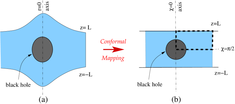
Figure 1: A spacelike slice of the black-hole spacetime. $(a)$ In the $\{r,z\}$ plane the black hole’s horizon is a curve with a spherical $S^{3}$ topology. $(b)$ There is a conformal freedom to transform the domain to $\{(r,z):|z|\leq L,~{}r^{2}+z^{2}\geq\rho_{h}^{~{}2}\}$. By fixing $\rho_{h}/L$ the domain is uniquely specified [21].

The fact that $x$ cannot be changed freely for a given solution implies that $x$ is a characteristic parameter analogous to the (normalized) total mass or the temperature even though it does not have a clear physical meaning. For example, if one enforces the horizon of a BH to be at a fixed radius set by some given $x$, it would be excessive to specify also the temperature. Conversely, specifying the temperature one does not have the freedom to constrain the location of the horizon [21].

In polar coordinates the reflecting boundary of the compact circle, $z=0$, is at $\chi=\pi/2$, but the periodic boundary, $z=L$, does not lie along a coordinate line in the $\{\rho,\chi\}$ plane. The treatment of this irregular boundary introduces a certain complication in the numerical scheme as described in section (4.1). Nevertheless, we believe that it is preferable to work in polar coordinates (2) and to have an irregular boundary at $z=L$, rather than work in rectangular coordinates $\{r,z\}$ and have an irregular boundary at the horizon. Intuitively, this is because we expect that the region near the horizon would become the region of the ’activity’ as $x$ increases.

For numerical reasons it would be convenient to use another angular coordinate

$$\xi=\cos(\chi)\ .$$ (5)

The benefit of using this coordinate is twofold. First, the irregular $z=L$ boundary has a particularly simple representation, $\rho=L/\xi$. Second, as we explain shortly, the coordinate singularity at the axis, $r=0$, becomes first order instead of second order.

2.2 Equations of motion

Our basic equations are the five-dimensional time independent vacuum Einstein equations. There are five equations in 5d: two are equations of motion for $A,C$, while variation with respect to the metric in the $(r,z)$ plane yields three additional equations. In the conformal ansatz one of them is an equation of motion for $B$ while the other two result from the gauge fixing. The equations can be combined in a way that three of them will take the form of elliptic equations, which we call the interior equations. The other two combinations that contain a hyperbolic differential operator will be termed ’the constraints’. These constraint equations are not independent as they are related to the interior equations via the Bianchi identities.

In order to obtain the interior equations we can follow the general procedure described in appendix A, or alternatively, use a suitable symbolic math application e.g. GRTensor [28] to evaluate the relevant quantities. In either route one obtains the interior equations which are the following combinations of the components of the Einstein tensor: ${\cal G}^{\theta}_{\theta}+{1/2}{\cal G}_{\chi}^{\chi}+{1/2}{\cal G}^{\rho}_{\rho}-2{\cal G}_{t}^{t}\ ,2{\cal G}^{\theta}_{\theta}-{2}{\cal G}_{\chi}^{\chi}-{2}{\cal G}^{\rho}_{\rho}+{\cal G}_{t}^{t}$ and ${\cal G}^{\theta}_{\theta}+{\cal G}_{\chi}^{\chi}+{\cal G}^{\rho}_{\rho}-{\cal G}_{t}^{t}$. They can be written respectively as

$$\triangle A + {2\partial_{\xi}A\over\rho^{2}}\left(-\xi+(1-\xi^{2})\partial_{\xi}C\right)+2\partial_{\rho}A\left({1\over\rho}+\partial_{\rho}C\right)=0,$$ (6)

$$\triangle B + \frac{2\,\partial_{\xi}A\,\left(\xi-\left(1-{\xi}^{2}\right)\,\partial_{\xi}C\right)}{A\,\rho^{2}}+\frac{2\,\partial_{\xi}C\,\left(\xi-{1\over 2}\left(1-{\xi}^{2}\right)\,\partial_{\xi}C\right)}{\rho^{2}}-$$ (7)

$$- \frac{2\,\partial_{\rho}C}{\rho}-\left({\partial_{\rho}C}\right)^{2}-\frac{2\,\partial_{\rho}A}{A}\left(\frac{1}{\rho}+\partial_{\rho}C\right)-\frac{1-e^{2\,B-2\,C}}{\rho^{2}\,\left(1-{\xi}^{2}\right)}=0\ ,$$

$$\triangle C - \frac{\partial_{\xi}A\,\left(\xi-\left(1-{\xi}^{2}\right)\,\partial_{\xi}C\right)}{A\,\rho^{2}}-\frac{4\,\partial_{\xi}C\,\left(\xi-{1\over 2}\left(1-{\xi}^{2}\right)\,\partial_{\xi}C\right)}{\rho^{2}}+$$ (8)

$$+ \frac{4\,\partial_{\rho}C}{\rho}+2\,\left({\partial_{\rho}C}\right)^{2}+\frac{\partial_{\rho}A}{A}\,\left(\frac{1}{\rho}+\partial_{\rho}C\right)+\frac{1-e^{2\,\left(B-C\right)}}{\rho^{2}\,\left(1-{\xi}^{2}\right)}=0\ .$$

Here we used the variable $\xi$ instead of $\chi$ and the Laplacian becomes $\triangle\equiv\partial_{\rho}^{2}+(1/\rho)\partial_{\rho}+(1/\rho^{2})\sqrt{1-\xi^{2}}\partial_{\xi}\left(\sqrt{1-\xi^{2}}\partial_{\xi}\right)$.

The constraint equations expand to

$${\cal G}_{\rho}^{\xi} \equiv \frac{{\sqrt{1-{\xi}^{2}}}}{\rho^{2}}\Big{\{}\frac{\partial_{\xi}A\,\left(\frac{1}{\rho}+\partial_{\rho}B\right)}{A}-\frac{2\,\xi\,\left(\partial_{\rho}B-\partial_{\rho}C\right)}{1-{\xi}^{2}}+\frac{2\,\partial_{\xi}B}{\rho}+2\,\partial_{\xi}C\,\partial_{\rho}B$$ (9)

$$+ 2\,\partial_{\xi}B\,\partial_{\rho}C-2\,\partial_{\xi}C\,\partial_{\rho}C+\frac{\partial_{\xi}B\,\partial_{\rho}A-\partial_{\rho\xi}A}{A}-2\,\partial_{\rho\xi}C\Big{\}}=0\,$$

$${\cal G}_{\rho}^{\rho}-{\cal G}_{\xi}^{\xi} \equiv -\frac{\partial_{\xi}A\,\left(\xi-2\,\left(1-{\xi}^{2}\right)\,\partial_{\xi}B\right)}{A\,\rho^{2}}+\frac{4\,\xi\,\left(\partial_{\xi}B-\partial_{\xi}C\right)}{\rho^{2}}-$$ (10)

$$- \frac{2\,\left(1-{\xi}^{2}\right)\,\left(2\,\partial_{\xi}B-\partial_{\xi}C\right)\,\partial_{\xi}C}{\rho^{2}}+\frac{\left(1-{\xi}^{2}\right)\,\partial_{\xi}^{2}A}{A\,\rho^{2}}+$$

$$+ \frac{2\,\left(-\xi\,\partial_{\xi}C+\left(1-{\xi}^{2}\right)\,\partial_{\xi}^{2}C\right)}{\rho^{2}}+\frac{\partial_{\rho}A\,\left(\frac{1}{\rho}+2\,\partial_{\rho}B\right)}{A}+$$

$$+ 2\,\left(2\,\partial_{\rho}B-\partial_{\rho}C\right)\,\left(\frac{1}{\rho}+\partial_{\rho}C\right)-\frac{\partial_{\rho}^{2}A}{A}-2\,\partial_{\rho}^{2}C=0\ .$$

Assuming that the interior equations are satisfied, the Bianchi identities ${{\cal G}_{\alpha}^{\beta}}_{;\beta}=0$, imply [9] the following relations between the constraint equations

$$\partial_{\zeta}{\cal U}+\partial_{\xi}{\cal V}=0\ ,$$

$$\partial_{\zeta}{\cal V}-\partial_{\xi}{\cal U}=0\ ,$$ (11)

where $\zeta=\log\rho.$, and we define the rescaled constraints ${\cal U}=\rho\sqrt{-g}\left({\cal G}_{\rho}^{\rho}-{\cal G}_{\xi}^{\xi}\right)/2\ ,{\cal V}=\rho^{2}\sqrt{-g}{\cal G}_{\rho}^{\xi}$ with $g\equiv det\ g_{\alpha\beta}$.

A nice feature follows[9]. The constraints ${\cal U}$ and ${\cal V}$ satisfy the Cauchy-Riemann (2.2) relations and hence each one of them is a solution of the Laplace equation. Hence, if one of the constraints is satisfied at all boundaries and the other at a single point along some boundary these constraints must be satisfied everywhere inside the domain. This fact will be referred hereafter as the “constraint rule”. In our implementation, following the choice in [9] we imposed ${\cal V}=0$ along all boundaries and ${\cal U}=0$ in the asymptotic region. It is important to check and confirm that the constraint ${\cal U}$ and ${\cal V}$ are satisfied everywhere for our numerical solutions, as we describe in section 4.2.

2.3 Boundary conditions and constraints

The interior elliptic equations (6-8) are subject to boundary conditions. In this section we describe the boundary conditions that define the problem completely. The integration domain is defined by $\{(r,z):0\leq z\leq L,~{}r^{2}+z^{2}\geq\rho_{h}^{~{}2}\}$, designated by the thick dashed line in Fig. 1. The boundary conditions are specified on the axis, at the horizon, in the asymptotic region and at the reflecting and periodic boundaries $z=L$ and $z=0$.

2.3.1 The $z=0$ and $z=L$ boundaries.

On the reflecting, $z=0$, and the periodic, $z=L$, boundaries we impose

$$\partial_{z}\psi=0,~{}~{}\psi=A,B,C.$$ (12)

While at the reflecting boundary this condition is simply $\partial_{\xi}=0$, at the periodic boundary its implementation is not direct, see section 4.1.1.

2.3.2 The $r=0$ axis.

Regularity of the metric on the axis (absence of a conical singularity) requires

$$B=C.$$ (13)

We use this equation as a Dirichlet condition for $B$. Equation (7) is not solved at the axis but it is only monitored there. For $A$ and $C$ the boundary conditions are automatic – on axis the (interior) equations for these functions become first order in derivatives normal to the boundary and have precisely the form of a b.c. Namely these equations are already incorporate b.c. and these do not need to be additionally specified. We term this an “automatic boundary condition”. This occurs because of our particular choice of the angular coordinate: we use $\xi$ instead of $\chi$. The axial symmetry of the problem dictates the $\partial_{r}=0$ condition for the metric functions, which translates to $\partial_{\chi}=0$ in spherical coordinates and $\sqrt{1-\xi^{2}}\partial_{\xi}=0$ in our coordinates. But on axis $\xi=1$ and hence this condition need not be imposed in our coordinates. While the coordinate singularity at the axis is quadratic, $\sim\sin(\chi)^{-2}$ when using $\chi$, it becomes linear $\sim(1-\xi)^{-1}$ when using $\xi$. With this advantage there is, however, a drawback: the metric functions are not differentiable at $\xi=1$. This requires a modification of the numerical scheme there, replacing the second order normal derivative of the interior equations by a first order one due to the considerations above as described in subsection (4.1).

2.3.3 The horizon

The horizon in our construction is located at $\rho_{h}=1$. For static solutions various notions of the horizon coincide – the event horizon (globally marginally trapped ), the apparent horizon (the outermost boundary of locally trapped surfaces) and the Killing horizon are all the same. The latter characterizes the horizon as a surface where

$$A\equiv 0.$$ (14)

This implies that along the horizon

$$\partial_{\xi}A=\partial_{\xi}^{2}A=0.$$ (15)

Even though the horizon normally is not singular (in curvatures) our equations do become singular there as the function $A$ vanishes. Now we describe how the physical regularity of the equations at the horizon gives boundary conditions for our functions. Expanding Eqs. (7,8) at the horizon we obtain the condition

$$\partial_{\rho}C=-1\ .$$ (16)

We still need a condition for $B$. We obtain this condition from the zeroth law of the black-hole mechanics (or thermodynamics), namely that for static solutions the surface gravity must be constant along the horizon (see for example [26]). The surface gravity along the horizon reads

$$\kappa=e^{-B}\partial_{\rho}A,$$ (17)

and the derivative of $\kappa$ along the horizon vanishes

$$\partial_{\xi}\kappa\sim\partial_{\xi}B-\frac{\partial_{\rho\xi}A}{\partial_{\rho}A}=0,\ \rm{at}\ \rho=\rho_{h}.$$ (18)

The upshot is that the boundary condition for $B$ can be obtained in one of the forms: either

$$B=C_{\xi=1}+\log{\left(\partial_{\rho}A\over\partial_{\rho}A_{\xi=1}\right)}\mid_{\rho_{h}},$$ (19)

from (17) and (13), or by integrating (18) outwards from the axis along the horizon. In our implementation we used the former form. However we have checked that a corresponding solution obtained by using the other option differs only slightly from our original one.

Note that the condition (18) implies that eqn. (9) (or ${\cal V}=0$) is guaranteed along the horizon, and vice versa.

We can get a different condition for $B$ as well. Examining eqn. (10) (${\cal U}=0$) one obtains the condition

$$\partial_{\rho}B=-1\ ,$$ (20)

which is necessary to ensure regularity of that equation along the horizon.

Altogether we now have too many conditions at the horizon: four boundary condition (14,16,19,20) for the three metric functions. However, as explained in [9] it is unnecessary to impose both constraints (${\cal U}=0$ and ${\cal V}=0$) at the same boundary, and actually it is necessary not to impose both in order to protect the problem from being over constrained.

Out of (19,20) we choose to impose (19). The condition (20) is satisfied for these solutions. The error becomes smaller with grid refinement and reaches $2\%$ for our finest grid. For the sake of completeness we also obtained solutions using (20) instead of (19). However, these solutions do not have a manifestly constant surface gravity. The variation of $\kappa$ along the horizon is small for small $x$, but can reach as much as $15\%$ for larger $x$ values. The overall difference between the two solutions is maximal near the horizon, being of the same $15\%$ magnitude. This difference fades off asymptotically and the constraints are still satisfied (with the same accuracy). We conclude that, in principle, it is possible to use the condition (20) to generate solutions, though the numerics should be refined further to reach an acceptable accuracy.

2.3.4 The asymptotic boundary.

Performing a Kaluza-Klein reduction one observes that the $z$-dependence of all fields is carried by massive KK-modes and hence fades off exponentially for large $r$. Thus, in the asymptotic region we can rewrite Eqs. (6-8) retaining only the $r$-dependence. Defining for convenience $\zeta\equiv log(r)$, we get

$$A^{\prime\prime}+A^{\prime}+2A^{\prime}C^{\prime}=0,$$

$$B^{\prime\prime}-B^{\prime}-2C^{\prime}-(C^{\prime})^{2}-{2A^{\prime}\over A}(C^{\prime}+1)-1+e^{2B-2C}=0,$$

$$C^{\prime\prime}+3C^{\prime}+2(C^{\prime})^{2}+{A^{\prime}\over A}(C^{\prime}+1)+1-e^{2B-2C}=0.\$$ (21)

Here the derivatives are calculated with respect to $\zeta$.

Asymptotic flatness at $r\rightarrow\infty$, requires $A-1=B=C=0.$ Linearizing the above equations we can solve them analytically (see appendix B) with these boundary conditions obtaining

$$A = 1-{a\over r}+{\cal O}({\log^{2}r\over r^{2}})\ ,$$ (22)

$$B = {b\over r}+{\cal O}({1\over r^{2}})\ ,$$ (23)

$$C = {c\log(r)\over r}+{\cal O}({1\over r})\ ,$$ (24)

where we also included the order of the corrections. Note the logarithmic term in C. This log-behavior is specific to 5d and indicates a very slow asymptotic fall-off. At leading order the coefficients in (22) are related by [23]

$$a-2b+c=0.$$ (25)

In the numerical solution one can impose the simplest Dirichlet conditions: $A-1=B=C=0$ at the asymptotic boundary. However, since in our numerical implementation the “infinity” boundary is located at a finite $r$ this option appears to be too crude. One can improve that by going to the next order in the expansion (22) and using (25) to get the refined conditions

$${d\over dr}(Ar)=1\ ,$$ (27)

$${d(Br)\over dr}=0\ ,$$

$$C=(-1+A+2B)\log(r)\ .$$ (28)

Here we have rewritten the conditions in a form convenient for a numerical implementation.

Unfortunately, we discovered that these linear conditions do not lead to a convergent scheme. To understand this, observe that the function with the slowest decay is $C$. In 5d, to resolve the difference between the first two terms in its asymptotic expansion with just $10\%$ accuracy one has to go to $r\sim exp(10)\rho_{h}$ – the log strikes hard! When the maximal $r$ is not extremely large (which is the case here for practical reasons) the non-linear corrections appear to be important for stabilizing the scheme [9].

Recall the “constraint rule” which will help us to derive a more subtle b.c. for C. In accordance with it we choose to enforce ${\cal V}=0$ along all boundaries. The rationale behind it is that this constraint is satisfied trivially at the axis and at the reflecting boundaries, asymptotically it decays exponentially fast, and only at the horizon this constrain is not trivial and yields (19). The second constraint must not be imposed at the horizon. At the axis it vanishes. Along the reflecting, $z=0$, and the periodic, $z=L$, boundaries this constraint does not carry any new information as it is just a linear combination of the interior equations. Hence, we are left with the asymptotic boundary. This boundary can be potentially dangerous since on one hand, $\left({\cal G}_{\rho}^{\rho}-{\cal G}_{\xi}^{\xi}\right)$ decays here and on the other hand the measure $\rho\sqrt{-g}$ blows up. This competitive behavior can result in an unpredictable ${\cal U}$. Thus, to guarantee that the constraint is satisfied, the natural and unique place to impose ${\cal U}$ is the infinity.

The upshot is that instead of the linear condition (28) we compute $C$ at the asymptotic boundary using the constraint equation ${\cal U}=0.$ By doing so we stabilize our algorithm and satisfy the “constraint rule”. Note that at the leading order the vanishing of ${\cal U}$ is consistent with the linear condition (28).

3 Thermodynamical and Geometrical Variables

In this section we briefly summarize the results from our previous paper [23] with a particular focus on the 5d case. Hereafter we work in units such that $G_{4}=1$.

At infinity

As stated in [23] (see also [16]) there are two energy-momentum charges that asymptotically characterize our configuration. These are the total mass, $m$ (or the dimensionless mass $\mu:=m/\hat{L}$), and what we called the tension. The latter is what an observer at infinity interprets as the tension of an imaginary string stretched along the compact circle. These charges can be calculated in terms of the numerical asymptotics [23]

$$\hat{L}\,\left[\begin{array}[]{c}\mu\\ \tau\\ \end{array}\right]={1\over 2\,}\left[\begin{array}[]{cc}2&-1\\ 1&-2\\ \end{array}\right]\,\left[\begin{array}[]{c}a\\ b\\ \end{array}\right].$$ (29)

The asymptotic mass can be calculated also in a direct way, using the free energy or the Hawking-Horowitz prescription [27] which gives the same result. In the linear regime, using the relation (25) in the above formulae one can express the physical charges in terms of any two of the numerical asymptotics.

At the horizon

The characteristic quantities at the horizon are the surface gravity (the temperature) and the area (the entropy) of the horizon. We have already defined the surface gravity in (17), and the temperature is proportional to it $T=\kappa/2\pi$. The entropy is related to the surface area by the famous Bekenstein-Hawking formula $S_{BH}=(A/4G_{N})$. In our coordinates the surface area reads

$$A_{3}=4\pi\rho_{h}^{3}\int_{-1}^{1}{e^{B+2C}}\sqrt{1-\xi^{2}}d\xi=4\pi(2L)^{3}x^{3}\int_{-1}^{1}{e^{B+2C}}\sqrt{1-\xi^{2}}d\xi\ .$$ (30)

Out of these thermodynamical variables a single dimensionless quantity can be formed

$$A^{(\kappa)}:=A_{3}\,\kappa^{3}.$$ (31)

In addition to the 3-area it is useful to define a pair of 2-areas of horizon sections. The equatorial 2-area section is given by

$$A_{\parallel}=4\pi\rho_{h}^{2}e^{2C}.$$ (32)

The 2-area of the section of the horizon along the axis is just

$$A_{\perp}=2\pi\rho_{h}^{2}\int_{-1}^{1}{e^{B+C}}d\xi.$$ (33)

With these 2-areas we define the eccentricity or the “deformation” of the horizon as

$$\epsilon={A_{\perp}\over A_{\parallel}}-1.$$ (34)

Finally we define “the inter-polar distance” which is the proper distance between the “north” and the “south” poles of the black hole calculated along the axis. This distance reads

$$L_{\mbox{poles}}=2\int_{\rho_{h}}^{L}dz\,e^{B},~{}~{}{\rm at}\ r=0.$$ (35)

Small black holes

For small black holes ($x\ll 1$) the tension should vanish, $\tau\simeq 0$, according to Myers [19]. In this case we have

$$\left[\begin{array}[]{c}a\\ b\\ \end{array}\right]\simeq\left[\begin{array}[]{c}4/3\\ 2/3\\ \end{array}\right]m,$$ (36)

In addition, in this limit we have

$$\mu\simeq{3\pi\over 8}x^{2}.$$ (37)

Small black holes are expected to resemble a 5d Schwarzschild black hole for which we have

$$\rm{5d~{}Schwarzschild:}~{}~{}~{}~{}~{}~{}A_{3}^{Sch}=16\pi^{2}\rho_{h}^{3},~{}~{}~{}A_{2}^{Sch}=16\pi\rho_{h}^{2},~{}~{}~{}\kappa={1\over 2\rho_{h}}.$$ (38)

More generally, the dimensionless variables can be expanded in a Taylor series as a function of $x$. It can be shown [24] that this expansion for $A^{(\kappa)}$ takes the form

$$A^{(\kappa)}=2\,\pi^{2}\,(1-3\cdot\zeta(2)\,x^{2}+\dots)~{},$$ (39)

where $\zeta(2)=\pi^{2}/6$ is the Riemann zeta function.

The analogous expansion for the eccentricity reads

$$\epsilon={8\over 3}\zeta(4)\,x^{4}+\dots\ .$$ (40)

Thus the prediction is that $\epsilon$ is positive, i.e. the black hole becomes prolate along the axis. This agrees with the intuitive expectation that the black hole should approach a string shape as it grows.

Other dimensionless quantities are the 3-area

$${\cal A}_{3}:={A_{3}\over\hat{L}^{3}}=2\pi^{2}x^{3}+\dots,$$ (41)

the surface gravity and the temperature

$$\bar{\kappa}:=\kappa\hat{L}=x^{-1}+\dots~{}~{}{\rm and}~{}~{}\bar{T}=2\pi x^{-1}+\dots\ .$$ (42)

and the polar distance

$$\ell:=L_{\mbox{poles}}/\hat{L}.$$ (43)

Smarr’s formula

The Smarr formula, also known as the integrated first law, is a relation between the thermodynamical variables of the problem both at the horizon and at infinity. It can be obtained either from the (differential) first law together with scale invariance, or by computing the Gibbons-Hawking free energy and combining it with the expression for the mass. We find [23]

$$A_{3}={8\pi\over\kappa}aL.$$ (44)

This formula relates the horizon characteristics $A_{3}$ and $\kappa$ with the asymptotic variable $a$, together with the dimensionful parameter $\hat{L}$. This formula is an important test for our numerical solutions.

A phase transition

One of the most important questions that we aim to answer is whether there is a maximal (dimensionless) mass of the black hole phase as anticipated in [8]. This is analogous to the minimal mass $\mu_{GL}$ of the uniform black string below which the string is classically unstable. What happens to a black hole more massive than the critical black hole is unknown and constitutes one of the puzzles of this system. The appearance of a critical mass should be signaled in the numerics by a very slow convergence and ultimately no convergence.

Given the asymptotic mass (29) of the black hole we can calculate the area of the corresponding black string of the same mass

$$A_{BS}=4\,\pi\,(2\,G_{4}\,m)^{2}\hat{L}.$$ (45)

or in a dimensionless form

$${\cal A}_{BS}:={A_{BS}\over\hat{L}^{3}}=16\pi\mu^{2}.$$ (46)

While the existence of a maximal mass designates a perturbative (tachyonic) instability, the solution with ${\cal A}_{BS}={\cal A}_{3}$ designates the point of the first order transition between the black hole and the black string phases. This transition can occur quantum mechanically, via tunneling, or by thermal fluctuations.

Summary

In our problem we define four thermodynamic measurable quantities namely the horizon 3-area, the surface gravity, the asymptotic mass, and the tension, as well as two geometric quantities the eccentricity of the horizon, and the inter-polar distance. The thermodynamic ones are related by the very non-trivial Smarr formula (44). The validity of this formula for our measurables is one of the most important tests for the numerics (in addition to usual numerical tests of convergence, constraint violation etc.) This is because the Smarr formula relates horizon variables, with asymptotic ones. Hence the degree of violation of this formula can serve as an indication of the global accuracy of the numerical method. Another important task is to check whether the measurables have the small $x$ asymptotics as expected/derived theoretically. We use dimensionless measurables: in this form the relations between them remain the same regardless of whether $\rho_{h}$ or $L$ are varied.

4 Numerical Implementation

In this section we describe our numerical algorithm for solving the system of partial non-linear elliptic equations (6-8). We estimate the rate of convergence of the numerics and check that the numerical errors are small and the constraints are satisfied. All our simulations were written in Fortran. The typical run time on a 2GHz Pentium4 PC took about 1-2 days. The output of the code was analyzed and visualized using Matlab.

4.1 The scheme

The numerical technique that is often implemented to solve partial elliptic equations is an iterative method, called ’Relaxation’, see e.g. [30, 31]. In this method the solutions are iteratively corrected, starting from some initial guess, until a desired accuracy is reached. For non-linear equations a modification is needed. Often an iterative Newton procedure is combined with relaxation to find solutions of non-linear equations [30, 31].

4.1.1 Numerical lattice and discretization

Near the horizon we employ polar coordinates $\{\rho,\xi\}$. Asymptotically, however, cylindrical coordinates are the natural choice. In order to use both we choose to divide our integration domain into two parts: (i) ’The nearby region’ near the horizon is covered by polar coordinates. (ii) ’The asymptotic region’ is glued to the nearby domain from the outer, far side and is covered by cylindrical coordinates. The two patches overlap in order to exchange information about the functions during the relaxation.

We discretize our equations on a lattice that covers the domain of the integration. We employ finite difference approximation (FDA) in which one replaces derivative operators by their discrete counterparts. The discrete operators are obtained by a formal Taylor expansion of functions at the grid points. We use an FDA which is second order in the grid spacing. For example, if $h$ is the stepsize in, say, the $\rho$ direction, which is sampled by index $j$, then the first and the second derivatives of a function $\psi$ at the lattice point $(k,j)$ are written to second order as

$$\partial_{\rho}\psi_{k,j}={\psi_{k,j+1}-\psi_{k,j-1}\over 2h}+{\cal O}(h^{3}),\ \partial_{\rho}^{2}\psi_{k,j}={\psi_{k,j+1}-2\psi_{k,j}+\psi_{k,j-1}\over h^{2}}+{\cal O}(h^{3}).$$ (47)

Analogous expressions can be found for all other derivatives.

Our second order FDA incorporates a 5 point computation molecule in the interior. Obviously, it would be nice to have the same feature also at the boundaries. In fact, we retain this feature at all boundaries but the axis through the introduction of false grid points. For the functions that have a Dirichlet boundary condition we solve inside the domain using data at the boundaries. This is the method for A and B on the horizon and for C asymptotically. To implement a Neumann condition we introduce false grid points located one stepsize outside the real boundaries. Since the normal derivative is given at the real boundary we define the function at the false grid points using the corresponding inner points. For example, at the horizon: $\partial_{\rho}C=(C_{k,j_{h}+1}-C_{k,j_{h}-1})/2\Delta\rho=-1$, where $j_{h}=1$ is the location of the horizon $\rho_{h}$; at the false point $(k,j_{h}-1)$ we have $C_{k,j_{h}-1}=C_{k,j_{h}+1}+2\Delta\rho$. Now we solve the equation on the real boundary just as for an interior point, using data at the false grid points. This is the method for C on the horizon and for A, B and C on the equator. The mixed Neumann-Dirichlet conditions for A and B, that are written in the form (27-27), are imposed in the same fashion. At the axis we have “automatic conditions” for A and C. Since the functions are not differentiable here in the $\xi$ direction we use one-sided (first-order) $\xi$-derivatives. Here our FDA, becomes 4 point and not completely second order as (47), see also the discussion in section 2.3.2.

The boundary $z=L$ is rather complicated in polar coordinates while being very simple in cylindrical ones. This brings us to a closer examination of the coordinate patches.

The nearby region: $\{\rho,\xi\}$ - patch.

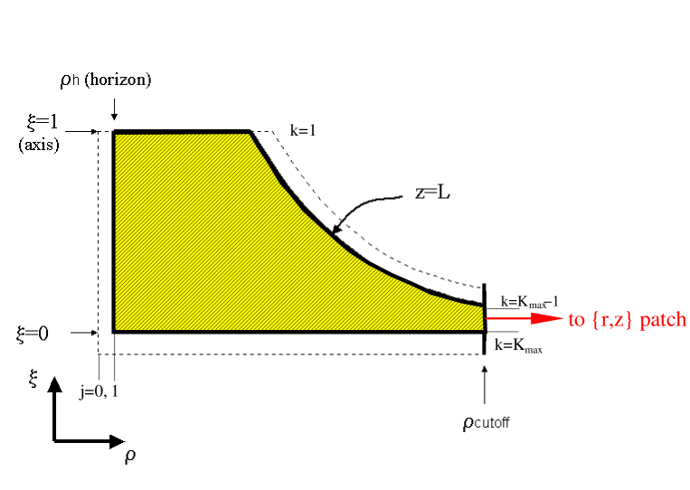
Figure 2: ’The nearby region’ of the integration domain covered by the polar coordinates $\rho,\xi$. The thin dashed lines mark the location of the false grid points used for numerical implementation of the Neumann or mixed Neumann-Dirichlet boundary conditions.

The lattice that covers this domain, see Fig.(2), has nodes at $k=1,...,K_{\rm max},K_{\rm max}+1$, in the $\xi$ direction, and nodes at $j=0,1,...,J_{\rm in}(k)$ in the $\rho$ direction. Here $J_{\rm in}(k)$ is the coordinate of the last point that lies within the boundary $z=L$, which is represented by the curve $\rho=L/\xi$. The false grid points here are introduced by the requirement that for each inner point there will be outer points that allow the implementation of the regular 5 point second order FDA scheme. This implies that at each $k$ the outer points occupy $J_{\rm in}(k)<j\leq J_{\rm out}(k)$ where $J_{\rm out}(k)=J_{\rm in}(k+1)$. During the relaxation we sweep the lattice from $k=1$ to $k=K_{\rm max}$ and from $j=0$ to $j=J_{\rm in}(k)$. At a given ray $k$ we correct the outer points at $k-1$ when we reach $j>J_{\rm in}(k-1)$ using the reflection b.c. To this end, for each outer point, ${\cal O}$, we find the corresponding inner point, ${\cal I}$, which is its mirror reflection with respect to the boundary ($(r,z)\to(r,2\,L-z)$). The functions at the inner point are obtained by a two dimensional interpolation from the surrounding points and then the corresponding outer point is updated. The important practical note is that the inner mirror points should be calculated only once prior to relaxation.

We choose fixed lattice spacings both in $\rho$ and $\xi$ directions. In the $\rho$ direction the grid is truncated at a finite $\rho_{\rm cutoff}$. For a specific $\xi-$stepsize, $\Delta\xi$, the maximal $\rho$ is

$$\rho_{\rm cutoff}={L\over\Delta\xi}.$$ (48)

The $\Delta\xi$ step is chosen such that $\rho_{\rm cutoff}\gg L$ (usually we took $\rho_{\rm cutoff}\sim 10L$.) Note that there are only two grid points on this far boundary in the $\chi$ direction for $\rho_{\mbox{cutoff}}$: one is at $K_{\rm max}-1$ and the other is at $K_{\rm max}$, see Fig. 2. Here the second patch of the integration begins.

The asymptotic region: $\{r,z\}$ - patch. This patch begins at $r=r_{\rm min}<\rho_{\rm cutoff}$ and extends up to $r=r_{\rm max}$. Note that there is a ’buffer zone’ where both patches overlap, see Fig.3. The variation of the functions in this portion of the integration domain is expected to be small provided that $\rho_{\rm cutoff}\gg L$. Thus, the lattice covering this portion does not need to be very dense. The grid has a simple rectangular geometry with uniform grid spacings. There are two false boundaries at $z=0,z=L$. At the near boundary, $r_{\rm min}$, all functions have Dirichlet b.c., the values being received from the ’nearby patch’. At the far boundary, $r_{\rm max}$,we implement the mixed Dirichlet-Neumann conditions (27-27) for A and B and evaluate C from the constraint ${\cal U}=0$. Since for practical reasons we were obligated to take finite, not too large $r_{\rm max}$ (we usually chose $r_{\rm max}\sim{\cal O}(1000)\rho_{h}$) the use of the non-linear condition for C is essential.

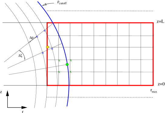
Figure 3: The asymptotic region is glued to the ’nearby patch’. The two patches overlap in order to exchange information about the functions during relaxation.

The equations are relaxed on both patches one after the other. First we sweep the lattice of the ’nearby region’ and then the lattice of the asymptotic region. Then the sweeps are iterated. The patches communicate. When sweeping the near patch we use the information from the far patch to supply boundary conditions at $\rho_{\rm cutoff}$. For example, see Fig. 3, the green point at $\rho_{\rm cutoff}$ can be obtained by e.g. a bi-linear interpolation from the points marked by crosses. While sweeping the far patch the boundary condition along the stitch at $r_{\rm min}$ come from the near patch. For example, the yellow point at $r_{\rm min}$ is obtained from the points marked by stars by a bi-linear interpolation.

To relax the equations we used a scheme which incorporates Newton iteration. To this end, at each grid point $(k,j)$, any function $\psi=A,B,C$ is updated according to

$$\psi^{\rm new}(k,j)=\psi^{\rm old}(k,j)-\omega{{\cal E}_{\psi}(k,j)\over\partial{\cal E}_{\psi}/\partial\psi(k,j)}\mid_{\rm old},$$ (49)

where ${\cal E}_{\psi}(k,j)$ is the FDA equation of motion for this $\psi$, and $\omega$ is a numerical factor.

The basic Gauss-Seidel algorithm uses $\omega=1$ and it leads to a very slow convergence. One way to speed up the performance is to use Successive Over Relaxation (SOR). The name originates from the fact that unlike the Gauss-Seidel scheme where the functions are corrected by exactly what they should be from the equations, in the SOR algorithm the correction is larger. The over-relaxation is managed by the relaxation parameter $1<\omega<2$. Sometimes, for non-linear equations it is better to use under-relaxation. In this case $0<\omega<1$ and the functions are under-corrected. The case $\omega>1$ ($\omega<1$) can be imagined as a sort of acceleration (friction). We implemented the SOR algorithm for our problem and found that the convergence rate is still unsatisfactory for dense grids.

4.1.2 Multigrid technique

The algorithm that we found to work well is what we loosely term here a Multigrid algorithm, see e.g. [31]. In the current simplified version of this method we solve the equations on several successive grids with doubled density. The basic idea of the Multigrid technique is simple – relax perturbations of different wavelengths on suitable lattices. Clearly, relaxation of a long-wave perturbation on a very fine grid will require many iterations, while if we first relax the perturbation on a course grid and use the solution as an input for the fine grid there is a chance to converge faster. Another advantage of using the Multigrid method is that there is a natural measure of accuracy. We can compare the solutions on different grids and see whether and how the differences decrease, indicating convergence and scaling of the truncation error. We used $4$ successive grids with halved stepsizes. Our implementation of the multigrid method was very simple. We just improved the solution going in one direction, namely passing from a coarse grid to a finer one. The original multigrid technique [31] incorporates motion in both directions allowing to relax newly excited modes on suitable grids. This two-directional method is expected to be much more effective and fast (but difficult to program.)

The Multigrid technique was implemented only on the ’nearby patch’. The asymptotic patch was chosen to have fixed grid spacings. This is because the variation of the fields is relatively small at large $r$ and there is no need for very dense grids. Note also that by decreasing the grid spacings in the nearby patch $\rho_{\rm cutoff}$ scales according to (48). Thus for each more dense grid $\rho_{\rm cutoff}$ is doubled. We, however, chose to keep the truncation radius constant, defined by the coarsest grid. In this case when the grid spacings were halved the number of the points on the boundary at $\rho=\rho_{\rm cutoff}$ was doubled.

In most of our simulations typical grid spacings in the asymptotic patch were $\Delta z\simeq 0.25-1.0$, and $\Delta r\simeq 0.075-0.25$. The typical grid spacings in the near patch were $\Delta\rho\simeq 0.1-0.25$ and $\Delta\xi\simeq 0.08-0.12$ for the coarsest grid. One can estimate the size of the lattice taking typical $L\sim 10\rho_{h},~{}\rho_{\rm cutoff},r_{\rm min}\sim 10L~{}~{}{\rm and}~{}~{}r_{\rm max}\sim 10\rho_{\rm cutoff}\sim 100L\sim 1000\rho_{h}$. In this case, the size, $N_{\xi}\times N_{\rho}$, of the coarsest polar grid is $10\times 1000$, while the finest grid is $160\times 16000$. The size, $N_{z}\times N_{r}$, of the asymptotic grid would have been $10\times 1000$, if the grid spacing in the $r$ direction were uniform.

4.1.3 Extracting measurables

Once we have a solution the horizon variables such as $\kappa,A_{3},A_{2}$ are calculated in a straightforward way from (17), (30) and (32,33) respectively . In order to obtain the asymptotic mass and the tension (29) we have to expand the metric functions asymptotically. We use fitting functions of a suitable form to obtain those coefficients. For example to find $b$ we need a quadratic fit in $r^{-1}$ for $B$ in the asymptotic region. To find $a$ a linear fit is usually sufficient for a good result. For $C$ we used a fit of the form $c_{1}\log(r)/r+c_{2}/r$. However, we were unable to find a reliable fitting for $C$. We associate this with the slow logarithmic decay.

4.1.4 Further developments

There are always compromises in numerics between the computation time and the accuracy of the calculation. This has to do with the grid density. Large grids mean small stepsizes and hence better accuracy provided that the FDA is stable, i.e. converges as a stepsize decreases. On the other hand, even if there were unlimited memory resources to store large arrays, such dense grids would result in extended CPU time that would be needed to sweep such large lattices. We tried different tricks to find a reliable compromise for this ’CPU-time vs. accuracy’ issue.

$\bullet$ A non-uniform asymptotic grid. Originally we implemented the asymptotic boundary conditions at $r_{\rm max}$, that is 30-50 $L$, or about 300-500$\rho_{h}$. However, we found that those values of $r_{\rm max}$ are not large enough to determine the mass with sufficient accuracy, especially for large values of $x$. Since in 5d the asymptotic fall-off is slow, (22), implementing the asymptotic boundary conditions at these $r_{\rm max}$ values is not accurate enough. Naturally, one would like to extend the grid to the larger $r_{\rm max}$. One way to do so is to add more points to the grid. However, in order to reach $r_{\rm max}$ larger by a certain factor than the original $r_{\rm max}$ the number of grid points must increase by the same factor. The same is true for the increase in the CPU time. Since we need $r_{\rm max}$ of order $\exp(10)\rho_{h}$, this makes the mere increase in number of points absolutely impractical.

We used another technique – a non-uniform grid spacings in the r-direction. The stepsizes were scaled in the following fashion

$$\Delta r_{i+1}=(1+\epsilon)\Delta r_{i}\ ,\ i=1,2,\ldots,N_{r}$$ (50)

Here $\epsilon$ is a small number that we usually took as $0.01-0.03$. In this case the coordinates of the mesh points in the $r$ direction form a geometric progression and it is possible to reach quite large values of $r_{\rm max}$ with a relatively small number of the mesh points. The discretized equations are now modified and the truncation error at a grid point $i$ scales as ${\cal O}(\epsilon\Delta r_{i})+{\cal O}(\Delta r_{i}^{2})$ rather than just ${\cal O}(\Delta r_{i}^{2})$, which is the case for a uniform grid with the spacing $\Delta r_{i}$. Provided $\epsilon$ is small this modification is not that different from a uniform FDA and does not cause problems. In the $z$-directions stepsizes were left uniform and hence the corresponding FDA derivative operators remained unchanged.

Keeping $\epsilon$ in the above range, in order to reach large enough $r$ (of order $\exp(10)\rho_{h}$)the grid turns out to be large enough to slow down the convergence notably. In practice, we could reach only $r_{\rm max}\simeq 500-800\rho_{h}$. The log strikes again.

$\bullet$ Additional relaxation near the horizon. This is needed in order to increase the accuracy of the calculation of $\kappa$ and the area of the horizon and its sections (30-33). Especially, the eccentricity (34) is sensitive to the accuracy of the area measurement. This relaxation operates over a finite portion of the mesh in the vicinity of the horizon. The boundary conditions along the horizon, axis and the equator are the same as before but along the outer boundary one uses just the Dirichlet boundary conditions that come from the main relaxation.

Over this region the metric functions were relaxed on two additional finer grids. One could suspect that the relaxation over a finite region would produce a mismatch along the stitch, that can be imagined as a kink or a ’ripple’ in the metric fields. However, we have checked that this is not the case, but rather the behavior of the functions was smooth. The maximal change in the functions relative to the previous grids occurred over a few mesh points near the horizon.

In addition, in a couple of runs we relaxed the equations over the entire integration domain on an additional 5th grid. When the area and the surface gravity, obtained in this case, were compared to the ones obtained in the relaxation over only a small region near the horizon, we found that the difference in both results is less then 0.1 %. The gain in computation time was however dramatic – hours vs. days.

$\bullet$ The over-(under-) relaxation parameter $\omega$. There is no universal algorithm to find the optimal $\omega$ that speeds up the convergence. Except for few very simple elliptic equations with simple boundaries there is no analytical prescription to pick such an optimal $\omega$. Often empirical estimates are the only way to find it. In our case the estimation of an optimal $\omega$ is even harder, since we need an omega for each of the three functions for both patches.

While we cannot be confident that the $\omega$-s we have used in our computations are the optimal ones, we can estimate the range of $\omega$ outside which the code slowed down or diverged. The choice $\omega_{A}=1-1.2,\ \omega_{C}=1-1.1,\ \omega_{B}=.5-1.$ in the nearby region, and, $\omega_{A}=\omega_{C}=1-1.2,\ \omega_{B}=.02-0.1$ in the cylindrical patch usually gave reasonable convergence rate. Some of these values depend on $x$. The most influential $\omega$ is $\omega_{B}$ in the asymptotic region: a slight deviation of its value from the narrow range ruins the convergence.

4.2 Testing the numerics

As usual in numerics one has to convince oneself that a particular numerical method produces trustable results. Before discussing our findings, we present in this section the evidence that our method performs well. We show that the numerical errors decrease sufficiently fast indicating a global convergence of the scheme and that the residual errors of the equations are small. In addition, in GR one has to ensure that the constraint equations are satisfied. We show that they are satisfied to a good extent. However, this ceases to be the case when $x$ is ’too large’. For $x$ above a certain value $x_{1}\simeq 0.20$, the convergence is slowed down, the constraints are violated significantly and the errors are not small for the results to be reliable. Additional accuracy estimates come from the Smarr formula, which our solutions satisfy with very good accuracy.

Numerical tests

We relax the equations on four grids with increasing density. For the first and coarsest grid we give some initial guess while when moving to a finer grid we start with the solution relaxed on the previous grid. The first thing that a good method must satisfy is independence of the initial guess. To achieve faster convergence we regularly used as the initial guess the uncompactified 5d Schwarzschild solution restricted to $|z|\leq L$. However, we checked that other initial guesses, such as flat spacetime glued to the horizon etc. relax to the same final solution. As an indicator of the accuracy during the relaxation we use the accumulative residual error defined as

$${\rm Res}\ \psi:={1\over 4^{n-1}}\sum_{k,j}{\left|\triangle\psi_{k,j}-{Src\psi}_{k,j}\right|}\ ,\rm{with}\ \psi=A,B,C\ ,$$ (51)

where $n$ is the grid number ($n=1$ is the coarsest) and the factor $4^{n-1}$ roughly compensates for the increase in the total number of grid points. The iterations on a particular grid were stopped when the residuals were reduced by a desired factor relative to some number, that we usually took as the initial residual calculated before relaxation on that grid. In Fig. 4 we depict the residuals on each grid. Their behavior suggests convergence.

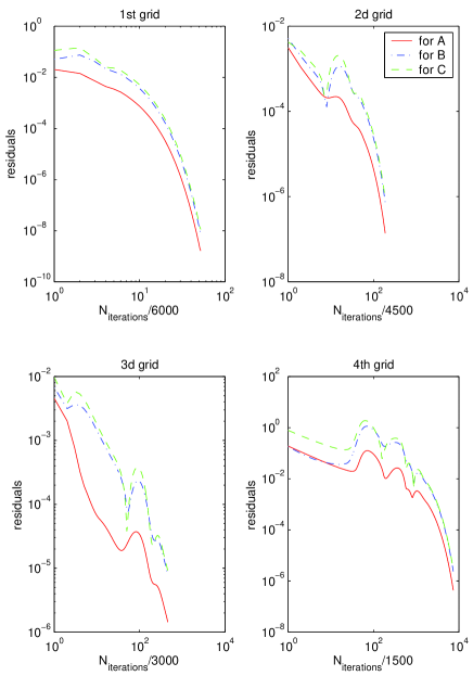
Figure 4: A log-log plot of the normalized residuals, $Res\ \psi$ vs. number of iterations, for $x=1/7$, implying convergence.

Note that the decrease of residuals is not monotonic all the way down. This implies that there are modes that are continuously excited and then decay. For small values of $x$ these modes are harmless, but have an imprint on the residuals’ decay – the oscillations. For larger $x$ values these modes are not suppressed – the oscillation increases their amplitude and then they finally diverge, see Fig.5.

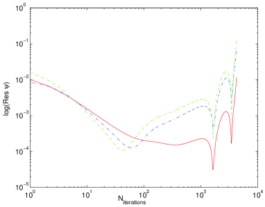
Figure 5: A log-log plot of the normalized residuals vs. number of iterations for $x>0.20$. After an initial convergence the solution diverges.

In addition to the convergence per grid we can use the benefits of the multigrid technique and check the convergence when moving between grids. We examine how much the solution is corrected when relaxed on different grids. To this end in Fig 6 we depict the differences between the solution on the $n$th grid and the solution obtained on the $n-1$, coarser grid. Since we used four grids there are three such pairs. We observe that the solution is corrected less on finer grids, as expected for a convergent method. Most of the corrections occur in the regions near the horizon and near the axis. In fact, this is the sort of behavior that allowed us to perform further relaxation with confidence even on finer grids in the vicinity of the horizon as described in the previous section.

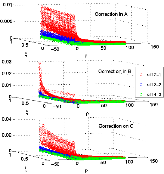
Figure 6: The corrections (or differences) in the elliptic equations when relaxed on different grids for $x=0.1$. One can see that the finer the grid, the less the solution is corrected.

We can also estimate the rate of convergence. Assuming that the solution converges to some $f^{\star}$ in the limit when the grid spacing goes to zero, we can write for the $n$th grid

$$f^{\star}=f_{n}+{\cal O}(h_{n}^{p}),$$ (52)

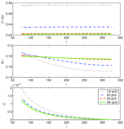
Figure 7: A run with $x=0.12$. Values of the functions at the equator in the asymptotic region for 4 grids. There is clear convergence.

where $h_{n}$ is the grid-spacing for this mesh. The rate of convergence is defined by the power $p$. If $p=1$ one speaks about linear convergence, if $p=2$ there is a quadratic convergence and so on. Taking differences between solutions on different grids and considering the fraction of these differences the value of $p$ can be estimated. Of course, the value of $p$ may vary at different points of the numerical lattice. However, one can calculate the minimal convergence rate by taking the minimum of those $p$. We find that in the asymptotic region the minimal convergence rates are $p_{A}\sim 3,\ p_{B}\sim 2,\ p_{C}\sim 3$ for the three metric functions. In the nearby region the convergence rate is also found to be at least quadratic for all functions. In the above estimates of $p$ we used only the three finest grids. The reason not to include the first grid is simple: its prime role is to perform a rough adjustment of the initial guess to the given boundary conditions. Hence, one expects that the solution on this grid is only a very crude approximation to the final solution. To guide the reader we plot in Fig. 7 the metric functions in the asymptotic region at the equator for four grids. The nice convergence there can be easily seen. When this is the picture we infer that our method converges nicely.

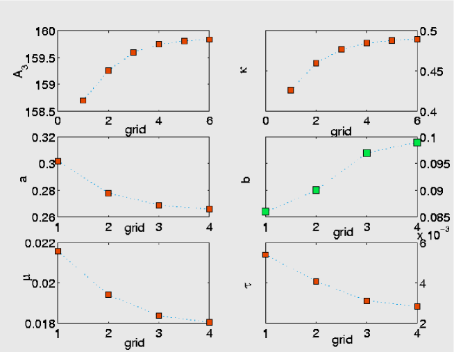
Figure 8: Four measurables and two asymptotics as a function of grid number for $x=1/12$. While the 3-area, $\kappa$ and $a$ converge nicely for all the $x$’s that we relaxed, $b$ does not. The absolute variation of the variables is small however. Note, however that the asymptotic charges, $\mu$ and $\tau$, converge as well.

Convergence of this kind occurred for intermediate values of $x$, roughly for $0.08\lesssim x\lesssim 0.15$. Outside this range the rate of convergence is still very good for all measurables but one. To envisage our point it is more convenient to use the numerical asymptotics $a$ and $b$, instead of our ’physical’ measurables, the asymptotic mass and tension. The typical behavior for our measurables as a function of the grid spacing is depicted in Fig. 8. While $A_{3},\kappa$ and $a$ are observed to reach their asymptotic values, $b$ is special – it does not seem to converge to a definite value. Note that the asymptotic charges, $\mu$ and $\tau$ seems to settle to definite values as well. Moreover, even though $b$ does not behaves monotonically, for small $x$ its value is limited to be within a narrow range, see Fig. 8. We will see below that the real problems of convergence begin when the fluctuations of $b$ are not small anymore. We refer to these fluctuations and the lack of accuracy in the measurements of $b$ as the “the b-problem”.

To get an idea of the overall accuracy of the numerics in the final solution, i.e. after relaxation on all four grids, we plot in Fig. 9 the normalized error in our elliptic equations. This error is defined at each mesh point $(k,j)$ as

$$\delta\psi_{k,j}\equiv{{\triangle\psi}_{k,j}+{Src\ \psi}_{k,j}\over\left|{\partial_{\rho}^{2}\psi}_{k,j}+{{1\over\rho}\partial_{\rho}\psi}_{k,j}\right|+\left|{{1\over\rho^{2}}\sqrt{1-\xi^{2}}\partial_{\xi}\left(\sqrt{1-\xi^{2}}\partial_{\xi}\psi\right)}_{k,j}\right|+\left|{Src\ \psi}_{k,j}\right|}$$ (53)

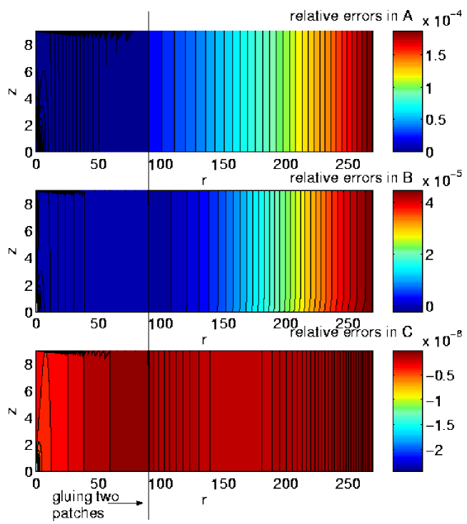
Figure 9: The normalized error in the elliptic equations, for $x=1/9$. This error defined in 53. It is encouraging that the maximal error is less then 0.02 %. We plotted here errors in both patches.

One observes that the relative errors are very small being less then $0.02\%$. As $x$ approaches $0.20$ the errors grow to a level of few percent.

Constraint equations

Additional insight into the accuracy of the method can be gained by studying the behavior of the constraint equations. It is clear that these must be satisfied for the actual solution of the Einstein equations. In Fig. 10 we plot the absolute value of the constraints on both grid patches. The figure shows that the constraints are not small in the far region of the polar patch. We believe that this loss of accuracy is due to the geometric pathology of the polar coordinates in the asymptotic region: the uniform grid cells in polar coordinates become very thin and prolonged when viewed in Cartesian coordinates. This causes a loss of accuracy, since asymptotically there are very few mesh points in the polar patch. Hence, an attempt to compute derivatives in the $z$-direction that are required from the physical point of view, gives inaccurate result. When we passed from grid to grid the constraints were satisfied better. When evaluating the constraints in the Cartesian patch we did not observe any pathologies. The constraints were small and decreased fast in the asymptotic region.

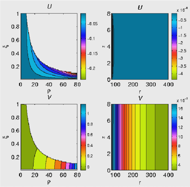
Figure 10: Absolute value of the constraint equations on both grid patches. While there is a loss of accuracy near the far boundary in the polar patch, both constraints are small in the Cartesian patch.

One gets a better insight for the constraints’ accuracy from examining the relative errors in them. These are defined similarly to Eqn. (53) and plotted in Fig. 11. One learns that the relative errors in the polar patch are indeed very small, being less then one percent, even though the absolute value of the constrains is not small. Thus, both Figs. 10 and 11 are complimentary and bring to light different aspects of the constraints behavior. The relative errors in the Cartesian patch are difficult to calculate because of the small absolute values of the constraints there. The absolute errors are small there and vary slowly, see Fig.10. Hence an attempt to evaluate the relative accuracy according to (53) fails, producing unpredictable results because of roundoff errors.

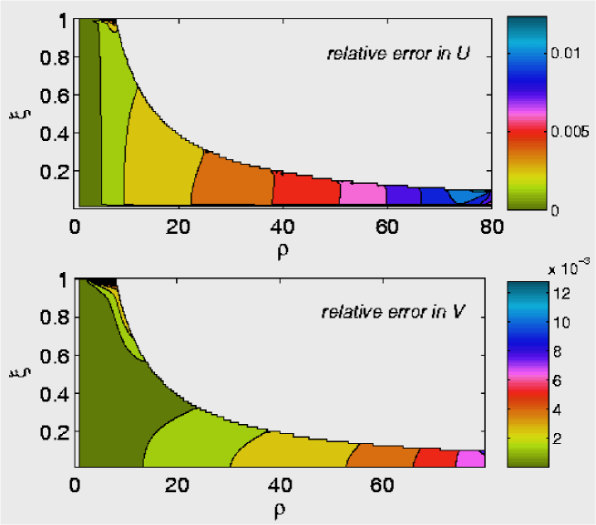
Figure 11: The relative errors in the constraints in the polar patch. These errors are small, being less then $2\%$, even though the absolute values of the constraints plotted in Fig.10 are not.

The fast convergence, small errors and small constraint violation are all attributes of the small $x$ runs. For certain $x$ the convergence rate became noticeably slower and the errors became uncontrollable. This was the $x$ when the ”problematic” asymptotic $b$ started to dominate. Even though we may expect positive tension $\tau>0$, namely $b<a/2$ in 5d $b$ reached $a/2$ and continued to grow for larger $x$. This designated the maximal $x$ for which we could fully trust our results, which is about $x\simeq 0.20$.

Applications of Smarr’s formula

Aside from numerical tests the Smarr formula (44) provides an important theoretical constraint. We found that Smarr’s formula is satisfied within $3-4\%$(!), see Fig. 12. We find a small systematic error: when evaluating $A_{3}\kappa/(8\pi aL)$, which should equal unity, we find that the mean value of the numerical points is about $0.97$ with a mean spread of less then $2\%$. This shows that our numerics produces systematically under-estimated values with a relatively narrow spread. In addition, there is a slight increase in accuracy when the asymptotic boundary is moved farther away. In this case the center of the distribution moves toward unity, though very slowly.

It is intriguing that the Smarr formula is satisfied with good accuracy for all our solutions, including those with a problematic $b$. Even for $x>0.20$ when the “b-dominance” triggered convergence problems this highly nontrivial formula continued to hold, see Fig.12. Together with Fig.8 this suggests that despite the fact that we could not determine the scalar charge accurately, the other three measurables are determined with good accuracy. Our working assumption will be that these measurables are trustable, even for $x>0.20$ up to the last convergent solution, at $x_{2}\simeq 0.25$, though in this regime the assumption becomes somewhat speculative.

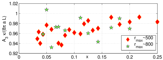
Figure 12: Testing the Smarr formula for two values of $r_{\rm max}$. The formula predicts $A_{3}\kappa/(8\pi aL)=1$. The mean value for distribution of point designated by diamonds is $.967$ with standard deviation of $.017$. The same for the stars is $.97$ and $.02$ correspondingly.

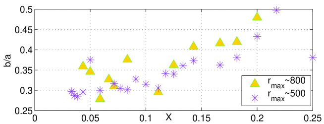
Figure 13: The ratio $b/a$ is expected to start at $0.5$ for $x\ll 1$, and decrease for larger $x$. Since $b=0$ for uniform black string, one might speculate that $b/a\rightarrow 0$ as $x$ increases. Here we see a different behavior. This behavior is not reliable since $b$ is problematic (at $30\%$ level) even at small $x$.

Let us discuss one more aspect of the “b-problem”. As we noted before even for small $x$ $b$ did not really converge, see Fig. 8. In addition, assuming positive tension, $\tau>0$, implies $b\leq a/2$, and the equality is obtained for small black holes that have vanishing tension. Since $b=0$ for a uniform string this suggests that for small $x$ $b/a$ should equal $\sim 1/2$ and should decrease to zero as $x$ increases. In Fig.13 we plot the ratio $b/a$. One observes that for small $x$ values the points are distributed around $1/3$ rather then around $1/2$. In accordance with our working assumption $a$ is calculated correctly, hence we estimate that the accuracy of the b calculation constitutes $30\%$, for small values of $x$. On the other hand, we have seen that for intermediate $0.08\lesssim x\lesssim 0.15$, $b$ does converge well. Hence, since the ratio $b/a$ is expected to decrease as $x$ increases, the measured value of $b/a\sim 0.3$ in this $x$ range can be trusted.

5 Results

One of the most important results of this work is that our numerical solutions are the first strong evidence for the existence of static black holes in a non maximally symmetric higher dimensional spacetime. We constructed a family of solutions parametrized by $x$, defined in (4). The horizon region of the solutions in this branch tend to the 5d Schwarzschild solution in the $x\rightarrow 0$ limit and become unstable for $x\rightarrow 0.25$. Even before that, at $x\simeq 0.20$, numerical errors were not small anymore. Our analysis is not capable to settle with certainty what has destabilized the algorithm. We tend to interpret this as originating from a physical tachyonic instability, though currently we are not able to determine the exact location of the transition point.

The geometry of the black holes

Let us examine the spacetime structure of a typical member of our family of solutions, with $x\sim 1/7$. In Fig. 14 we use contour plots to visualize the behavior of the metric functions and gain some insight for the geometry.

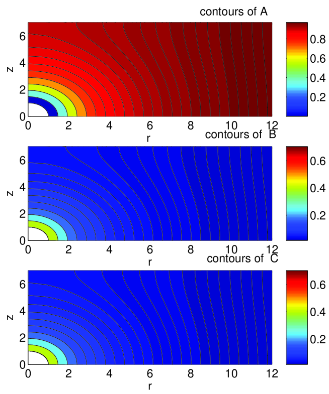
Figure 14: Contours of the metric functions for $x=1/7$. The black hole is located at the left bottom corner. The vertical periodic direction marked by $z$. Note the change of the topology of the contours. Near the horizon they are spherical while far away the contours become cylindrical, indicating translation invariance along $z$ at infinity.

The function $A$ vanishes at the horizon and it approaches unity asymptotically. The functions $B$ and $C$ decay smoothly from a finite value at the horizon to zero at infinity. One observes as well that the $z$-dependence disappears fast as one gets away from a black hole. In addition, one learns that the contours intersect all the boundaries at an angle of 90 degrees: the periodic at $z=L$, the reflecting at $z=0$, and the $r=0$ axis. This shows that the numerical scheme performs well at the boundaries.

The proper deformation or eccentricity of the horizon (34) is depicted in Fig. 15. Below $x\simeq 0.05$ the values that we obtain are randomly distributed around zero with magnitudes of $10^{-6}$, hence we concluded that the black hole is spherical to better then $10^{-6}$ at this regime. The main tendency to be noted in the figure is that $\epsilon>0$. This means that as $x$ grows the black hole becomes prolate along the axis, tending to a string-like form, as one could expect intuitively. Another interesting feature is that the last black hole that we have obtained (with $x\simeq 0.25$) is only slightly deformed, with $\epsilon\simeq 6.5\cdot 10^{-3}$. Comparing with the theoretical quantitative prediction (40), where ${8\over 3}\zeta(4)\simeq 2.89$, we see that the numerical “experiment” agrees exactly. Moreover, the axis intersection value $-3.5\cdot 10^{-5}$ agrees with the expected zero up to the numerical errors, see Table 1. We note that although the agreement looks “too good”, a fairly good agreement persists also for fits on smaller neighborhoods of $x=0$.

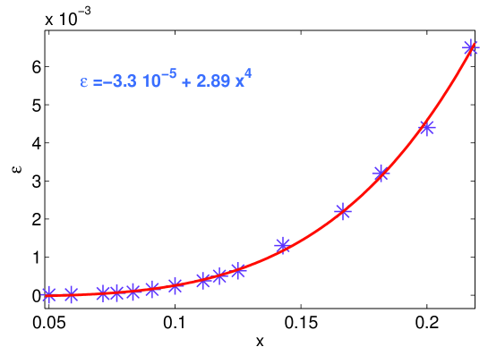
Figure 15: Eccentricity or deformation of the horizon. It stays very small up to $x\simeq 0.25$, where our code becomes unstable. The coefficient of proportionality agrees exactly with (40)!

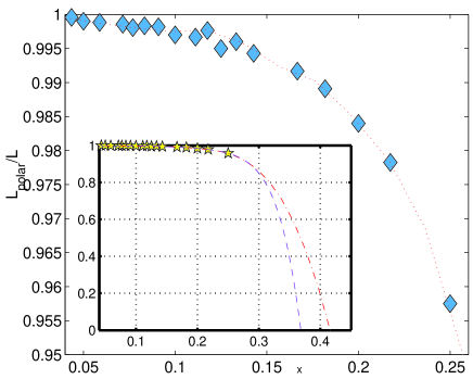
Figure 16: The normalized inter-polar proper distance starts at 1 for small $x$ and decreases as $x$ grows. Note the surprisingly small rate of decrease. The insert contains a speculative extrapolation. If the latter is correct, the “north” and the “south” poles of the black hole will touch at $x\simeq 0.4$. The two extrapolation lines correspond to a spline (dash-dotted) and to a 8-degree polynomial (dashed).

The (normalized) inter-polar distance (43) is plotted in Fig. 16. One observes that $\ell$ decreases so that the “north” and the “south” poles of the black hole approach each other. This decrease however is slow, such that just before the last $x\simeq 0.25$, $\ell$ is still very far from vanishing. This suggests several possibilities: (1) Our numerical solution crashes due to uncontrollable errors, and hence at $x\simeq 0.25$ there is not really a tachyonic instability. In this case the possibility that $\ell$ will shrink to zero and the phase transition will be smooth is not precluded by our analysis. (2) The point $x\simeq 0.25$ is in the vicinity of the real phase transition and $\ell$ does not drop to zero, signaling a non-smooth phase transition. This possibility was advocated in [8]. It is interesting to note that such features as the finiteness of $\ell$ and the smallness of the eccentricity, just before the transition, were obtained in [14] for momentary-static black hole solutions. The small $x$ behavior of $\ell$ is surprising. Neglecting the effect of the black hole on the spacetime metric one would expect a linear decrease. However, as the figure shows the decrease is much slower. This phenomena is not understood yet. It looks like as if the mass of the BH expands space in such a way that compensates almost exactly for its size. This effect can be called an “Archimedes law for caged black holes”.

In an insert in Fig. 16 we plotted a possible extrapolation of the measured $\ell$. If this extrapolation is correct then the poles will touch for $x\sim 0.4$.

Thermodynamical variables

Our prime thermodynamical variables are depicted in Fig. 17.

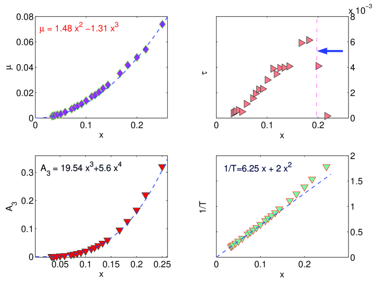
Figure 17: The dimensionless mass, tension, 3-area and the temperature along the found branch. The dashed line designates the corresponding variables for the 5d Schwarzschild solution. The shown equations are an approximation for small $x$, the coefficients with the fitting error are given in Table. 1.

We see that in the small-$x$ limit all variables tend to their Schwarzschild values, designated by the thick dashed line. The uncompactified Schwarzschild solution appears to be a smooth limit of the near horizon region of the caged black holes under discussion. One notes that three of the four thermodynamical variables have a smooth behavior all the way up to $x\simeq 0.25$, while the fourth one (the tension) is somewhat less consistent and for $x\gtrsim 0.20$ its behavior is strange. This is in agreement with our observations in section 4.2. We have argued, based on the success of the Smarr formula, that the three prime measurables ${\cal A}_{3},T,a$ are robust, while the fourth variable, $b$, has an uncertainty of about $30\%$ based on convergence problems and disagreement for small $x$. This rather large error is presumably confined to $b$ due to an approximate decoupling of equations in the asymptotic region, see appendix B. Moreover, it is this decoupling that allows the success of Smarr’s formula. Due to different relative weights that the asymptotics $a$ and $b$ have in the mass and the tension calculation, see (29), $\mu$ appears smooth in Fig. 17, while $\tau$ does not.

For small $x\ll 1$ one can consider a Taylor expansion of the thermodynamical variables in powers of $x$. We can attempt to extract the expansion coefficients by fitting the measurables with polynomials. We applied a fitting procedure for the first 8 to 10 solutions for which $x\leq 0.11$. The expansion coefficients together with the numerical errors are given in Table 1, as well as the expansion coefficients of $A^{(\kappa)}$, defined in Eq. (31) and plotted in Fig.18.

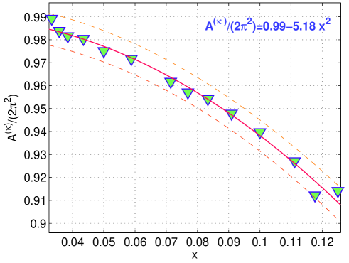
Figure 18: $A^{(\kappa)}/(2\pi^{2})$ for small $x$. The leading correction agrees well with (39)! The confidence bounds are depicted. No other Taylor coefficients could be extracted reliably.

For completeness, the corresponding data for $\epsilon$ is also added to that table. Everywhere the numerical coefficients are given with the estimated error. This is defined here by the variation of the coefficients of the fitting functions, while allowing the fit to vary within the $95\%$ confidence range, which is illustrated in Fig.18.

	Fitting Formula	$f_{1}\pm\delta f_{1}$	$f_{2}\pm\delta f_{2}$	Theoretical $f_{1}$
$\mu$	$f_{1}x^{2}+f_{2}x^{3}$	$1.48\pm.07$	$-1.3\pm 0.6$	$3\pi/8\simeq 1.18$
${\cal A}_{3}$	$f_{1}x^{3}+f_{2}x^{4}$	$19.54\pm.08$	$5.6\pm 1.0$	$2\pi^{2}\simeq 19.74$
$T^{-1}$	$f_{1}x+f_{2}x^{2}$	$6.25\pm.05$	$2.0\pm.12$	$2\pi\simeq 6.28$
$A^{(\kappa)}/(2\pi^{2})$	$f_{1}+f_{2}x^{2}$	$.99\pm.004$	$-5.18\pm.4$	$f_{1}=1,~{}f_{2}\simeq-4.93$
$\epsilon$	$f_{1}+f_{2}x^{4}$	$-(3.3\pm 4.8)\cdot 10^{-5}$	$2.89\pm.06$	$f_{1}=0,~{}f_{2}\simeq 2.89$

Table 1: The numerically computed expansion coefficients of the thermodynamical and geometric variables. Theoretical predictions for the leading terms are listed in the last column.

We can compare now the expansion coefficients to the theoretical predications that are summarized in section 3. The leading expansion coefficients, which are listed in the last column of Table 1, are confirmed with a good confidence, aside for the mass, $\mu$, for which the numeric and the theoretical numbers differ by about $20\%$. This is the imprint of the poor $b$ behavior, since $b$ is a part of the formula (29) for the mass. The higher order corrections to $\epsilon$ and $A^{(\kappa)}$ match beautifully with new theoretical results [24, 23]. Other coefficients have a somewhat greater uncertainty (sometimes tens of percents). Since we do not have a theoretical insight, and because of the large numerical errors we regard them as tentative.

We conclude that in the small $x$ regime most of our measurables are very robust. We argue as well, that the problematic $b$ affects $\mu$, but it is even more influential in the tension calculation, see Eqn.(29). The latter is depicted in Fig. 17. In this plot the demarcation line corresponds to $x\simeq 0.20$. In our numerical relaxation we observed a slow down of convergence and a loss of accuracy when approaching $x\simeq 0.20$. This fact finds its vivid representation in the tension plot. The points beyond the demarcation line drop suddenly and the tension vanishes at $x\simeq 0.22$.

Based on the success of the integrated first law our working assumption is that the entropy, temperature and the numerical asymptotic $a$ are robust not only for small $x$ but for all the solutions, up to $x\simeq 0.25$, see the discussion in the end of previous section 4.2. Moreover, one may observe that even though the mass evaluation is very sensitive to $b$ the main contributor is still $a$: $\mu=(a-b/2)/\hat{L}$. Hence, as long as $b<a/2$, which is the case here, see Fig.13, one may assume that the mass calculation is accurate within $20-25\%$ limits. This will be our second, more speculative, assumption. Using it, one can question what additional information can be extracted from out data. Addressing this question we ask: is there

A phase transition?

We interpret the instability of the numerics as a manifestation of a real physical tachyonic instability, which slows down our scheme for $x\gtrsim x_{1}\simeq 0.20$, and which finally ruins it completely at $x_{2}\simeq 0.25$. Examining the (dimensionless) masses corresponding to the above two $x$-values, we find that $\mu_{1}\simeq 0.047$ and $\mu_{2}\simeq 0.074$ are not that far from the GL critical mass, $\mu_{\rm GL}\simeq 0.070$. Since a priori, the various instability masses in the system are expected to be of the same order, this coincidence is rather suggestive. This is another evidence to our assumption that we are approaching the real physical instability.

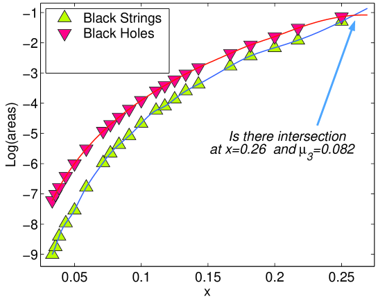
Figure 19: The logarithm of the dimensionless area of the black hole, ${\cal A}_{3}$, and black string, ${\cal A}_{BS}$, with the same mass. The continuous lines show extrapolation of the data to larger $x$ values, suggesting an intersection and a first order phase transition at $x\simeq 0.26$.

The existence of a maximal mass designates perturbative, classical instability. On the other hand, once the entropies of the two solutions are equal for a given mass, a first order phase transition between the two phases can take place. This transition will occur either by quantum mechanical tunneling or by thermal fluctuations. In Fig. 19 we depict the logarithm of the dimensionless areas ${\cal A}$, for the two phases: the black hole and the black string, where ${\cal A}_{BS}$, is computed for the same mass, $\mu=\mu(x)$. Our data does not show a crossing of the areas. However, a naive extrapolation of the data points, marked by the solid lines in Fig.19, indicates an intersection just above our last BH namely at $x\simeq 0.26$. For this value the mass is $\mu_{3}\simeq 0.082$, which is also of order of the critical GL mass.

Note that the extrapolated $\mu_{3}$ is slightly larger then our instability mass, $\mu_{2}$, while the opposite is expected for a first order phase transition. However, this inequality is not numerically significant: due to the high degree of uncertainties near the instability point we cannot estimate well the critical mass $\mu_{2}$. In addition one cannot expect that $\mu_{3}$ is evaluated accurately, since its value will depend strongly on several (not very accurate) last points in Fig.19.

It is important to determine whether $\mu_{2}<\mu_{\rm GL}$. If so there must be a third stable phase to which the black hole decays, for instance the stable non-uniform string [3]. However, we expect $\mu_{2}>\mu_{\rm GL}$.

6 Future directions

We conclude by pointing out some future directions

• Higher dimensions $d>5$. In this paper we presented a 5d numerical implementation of the ideas outlined in our previous paper [23]. In principle, after some slight modifications the code can be applied to a higher dimensional problem. While we expect that the instability, being physical, would still be present there, we hope to improve the accuracy of the critical mass estimation.

  We hope that the accuracy will improve in this case due to faster asymptotic decay. In addition, as we described in section 4.1.4 faster asymptotic decay implies smaller $r_{\rm max}$, hence smaller number of grid points and therefore faster operation of the code, which is now frustratingly long (1-2 days).

• Improving the performance of the method. One can try to improve further the algorithm, by e.g. using the full multigrid technique that incorporates motion up and down grid numbers. In order to improve the accuracy near the axis we could use as an angular coordinate the angle $\chi$ instead of $\xi=\cos(\chi)$. The benefit is that the axis is approached faster in the $\chi$ coordinates, and so there are more grid points near it. The drawbacks (as we explained in the text) are that the coordinate singularity would be second order and the periodic boundary,$z=L$, would loose its particularly simple representation $\rho=L/\xi$.

• Another choice of coordinates. The metric ansatz that we used here contains three functions. It would be interesting to try and implement the coordinates suggested in [7] and substantiated in [10, 17]. In these coordinates the number of functions reduces to two, and moreover they interpolate smoothly between spherical coordinates in the horizon region and cylindrical ones asymptotically, thus eliminating the need for the two coordinate patches.

Acknowledgments

It is a pleasure to thank J. Bahcall for suggesting this collaboration. BK thanks T. Wiseman and D. Gorbonos for discussions and collaboration on related issues.

The authors are supported in part by the Israeli Science Foundation.

Appendix A Equations of motion and boundary conditions on a d-cylinder

In this appendix we derive the equations of motion on a d-dimensional cylinder, ${\mathbb{R}}^{d-2,1}\times{\bf S}^{1}$ and the corresponding boundary conditions

The most general ansatz which is time independent, time reversal symmetric (“static”) and with axial $SO(3)$ symmetry is

$$ds^{2}=-\exp(2\hat{A})dt^{2}+d\sigma^{2}(r,z)+\exp(2\hat{C})d\Omega_{d-3}^{~{}2}$$ (54)

where $z$ and $z+\hat{L}$ are identified , $~{}d\Omega_{d-3}^{2}$, is the $d-3$ sphere, $\hat{A},\hat{C}$ are functions of $(r,z)$ and $d\sigma^{2}(r,z)$ is an arbitrary metric in the $(r,z)$ plane. Note that we dropped for now the $r^{2}$ prefactor in front of $\exp(2\hat{C})$. Classically the problem scales with $\hat{L}$, and so we can set $\hat{L}=2\pi$ and it can always be restored by dimensional analysis.

We need the expression for the Ricci scalar of a fibration. For $ds^{2}=ds^{2}_{X}+\exp(2F(x))ds^{2}_{Y}$ one has

$$R=R_{X}+\exp(-2F)R_{Y}-d_{Y}(d_{Y}+1)(\partial F)^{2}-2d_{Y}\triangle(F)$$ (55)

where the Laplacian is given by $\triangle(F)=\mbox{det}(g)^{-1/2}\partial_{\mu}(g^{\mu\nu}\mbox{det}(g)^{1/2}\partial_{\nu}F)$, grad squared is $(\partial F)^{2}=g^{\mu\nu}~{}\partial_{\mu}F~{}\partial_{\nu}F$ and $d_{X}=\mbox{dim}(X),~{}d_{Y}=\mbox{dim}(Y)$ (we normalized the Ricci scalar by $R=R_{ijij}$ so that $R_{{\bf S}^{d}}=d(d-1)$).

The d-dimensional Ricci scalar is

$$R_{d} = R_{2}-2(\partial\hat{A})^{2}-2\triangle\hat{A}+(d-3)\,(d-4)\,e^{-2\hat{C}}$$ (56)

$$- (d-3)\,(d-2)\,(\partial\hat{C})^{2}-2\,(d-3)\,\triangle\hat{C}-2(d-3)(\partial\hat{A})(\partial\hat{C})$$

While deriving this formula one has to be careful to consider the $\hat{A},~{}\hat{C}$ fibration step-wise, and thereby get the cross term $-2(d-3)(\partial\hat{A})(\partial\hat{C})$ in addition to $-2\triangle(\hat{A}+(d-3)\hat{C})$.

The gravitational action is

$$I={\Omega_{d-3}\over 16\pi G_{N}}\int dtdV_{2}~{}e^{\hat{A}+(d-3)\,\hat{C}}R_{d},$$ (57)

where $G_{N}$ is the d-dimensional Newton constant, $dV_{2}=\sqrt{-g}_{(r,z)}\,drdz$, $\Omega_{d-3}$ is the area of the unit $d-3$ sphere, and from now on we will drop the prefactor ${\Omega_{d-3}\over 16\pi G_{N}}\int dt$.

After integrating by parts we get

$$I=\int dV_{2}~{}e^{\hat{A}+(d-3)\hat{C}}[R_{2}+(d-3)(d-4)e^{-2\hat{C}}+(d-3)(d-4)(\partial\hat{C})^{2}+2(d-3)(\partial\hat{A})(\partial\hat{C})].$$ (58)

Now we need to fix the metric ansatz in the 2d $(r,z)$ space. One can use diffeomorphism invariance to put it in the conformal form

$$ds^{2}=-\exp(2\hat{A})dt^{2}+\exp(2\hat{B})(dr^{2}+dz^{2})+\exp(2\hat{C})d\Omega^{2}.$$ (59)

The formula for the Ricci scalar of a conformally transformed metric $g^{ab}=\exp(2\hat{B})\tilde{g}^{ab}$ reads [26]

$$R_{d}=e^{-2\hat{B}}[\tilde{R}_{d}-2(d-1)\partial_{ii}\hat{B}-(d-1)(d-2)\partial_{i}\hat{B}\partial_{i}\hat{B}].$$ (60)

Hence in 2d with the conformally flat metric we get

$$R_{2}=-2e^{-2\hat{B}}\partial_{ii}\hat{B}.$$ (61)

The action (without second derivatives after integration by parts) is

$$I=\int dr~{}dz[(d-3)(d - 4)e^{\hat{A}+2\hat{B}+(d-5)\hat{C}}+e^{\hat{A}+(d-3)\hat{C}}(2\,\partial_{i}\hat{A}\partial_{i}\hat{B}+2(d-3)\partial_{i}\hat{A}\partial_{i}\hat{C}$$ (62)

$$+ 2(d-3)\partial_{i}\hat{B}\partial_{i}\hat{C}+(d-3)(d-4)\partial_{i}\hat{C}\partial_{i}\hat{C})].$$

The equations of motion are

$$\hat{A}: \partial_{ii}(\hat{B}+(d-3)\hat{C})+{(d-3)(d-2)\over 2}(\partial_{i}\hat{C})^{2}-{(d-3)(d-4)\over 2}e^{2\hat{B}-2\hat{C}}=0$$ (63)

$$\hat{B}: \partial_{ii}(\hat{A}+(d-3)\hat{C})+(\partial_{i}(\hat{A}+(d-3)\hat{C}))^{2}-(d-3)(d-4)e^{2\hat{B}-2\hat{C}}=0,$$ (64)

$$\hat{C}: \partial_{ii}(\hat{A}+\hat{B}+(d-4)\hat{C})+(\partial_{i}\hat{A})^{2}+(d-4)(\partial_{i}\hat{A})(\partial_{i}\hat{C})$$ (65)

$$+{(d-3)(d-4)\over 2}(\partial_{i}\hat{C})^{2}-{(d-4)(d-5)\over 2}e^{2\hat{B}-2\hat{C}}=0.$$

where the grad squared is defined here without a metric factor $(\partial_{i}\hat{A})^{2}=(\partial_{i}\hat{A})(\partial_{i}\hat{A})$.

We find it convenient to redefine

$$\hat{B}\rightarrow B,~{}~{}e^{\hat{C}}\rightarrow e^{C}r~{}~{}{\rm and}~{}~{}e^{\hat{A}}\rightarrow A.$$

Solving for $\triangle(A),\,\triangle(B),\,\triangle(C)$ we obtain the equations of motion, which in $\{r,z\}$ coordinates are

$$\triangle A+(d-3){\partial_{r}A\over r}+(d-3)(\partial_{r}A\partial_{r}C+\partial_{z}A\partial_{z}C)=0,$$ (66)

$$\triangle B-{(d-3)(d-4)\over 2}\partial_{r}C\left({2\over r}+\partial_{r}C\right)-{(d-3)\over 2}\partial_{z}C\left((d-4)\,\partial_{z}C+2{\partial_{z}A\over A}\right)$$

$$-(d-3){\partial_{r}A\over A}\left({1\over r}+\partial_{r}C\right)-{(d-4)(d-3)\over 2}{1-e^{2B-2C}\over r^{2}}=0,$$ (67)

$$\triangle C+(d-3)\partial_{r}C\left({2\over r}+\partial_{r}C\right)+\partial_{z}C\left((d-3)\,\partial_{z}C+{\partial_{z}A\over A}\right)$$

$$+{\partial_{r}A\over A}\left({1\over r}+\partial_{r}C\right)+(d-4){1-e^{2B-2C}\over r^{2}}=0,$$ (68)

where $\triangle:=\partial_{r}^{2}+\partial_{z}^{2}$. These equations can be transformed to polar coordinates, $\{\rho,\chi\}$, where we have

$$\triangle A + (d-3){\partial_{\rho}A\over\rho}+(d-3)\partial_{\rho}A\partial_{\rho}C+{(d-3)\partial_{\chi}A\over\rho^{2}}(\partial_{\chi}C+{\rm ctg}(\chi))=0,$$ (69)

$$\triangle B - {(d-3)(d-4)\over 2}\left[\partial_{\rho}C\left({2\over\rho}+\partial_{\rho}C\right)+{\partial_{\chi}C\over\rho^{2}}\left(\partial_{\chi}C+2{\rm{ctg}}(\chi)\right)\right]-$$

$$- {(d-3)\over A}\left[\partial_{\rho}A\left(\partial_{\rho}C+{1\over\rho}\right)+{\partial_{\chi}A\over\rho^{2}}(\partial_{\chi}C+{\rm ctg}(\chi))\right]-$$

$$- {(d-4)(d-3)\over 2}{1-e^{2B-2C}\over\rho^{2}\sin(\chi)^{2}}=0,$$

$$\triangle C + (d-3)\left[\partial_{\rho}C\left({2\over\rho}+\partial_{\rho}C\right)+{\partial_{\chi}C\over\rho^{2}}\left(\partial_{\chi}C+2{\rm{ctg}}(\chi)\right)\right]+$$ (71)

$$+ {1\over A}\left[\partial_{\rho}A\left(\partial_{\rho}C+{1\over\rho}\right)+{\partial_{\chi}A\over\rho^{2}}(\partial_{\chi}C+{\rm ctg}(\chi))\right]+(d-4){1-e^{2B-2C}\over\rho^{2}\sin(\chi)^{2}}=0.\$$

Here $\triangle:=\partial_{\rho}^{2}+(1/\rho)\partial_{\rho}+(1/\rho^{2})\partial_{\chi}^{2}$ is the flat Laplacian in the polar coordinates.

These are elliptic equations, and as such they are subject to boundary conditions. One can see that the boundary conditions are basically dimension independent. The only difference will appear at the boundary at infinity, because of the different fall-off rate of the functions. Asymptotic flatness singles out natural radial coordinate at infinity, $r\sim r_{\rm Schwarzschild}$. In [23] we found for $d>5$

$$1-A = {a\over r^{d-4}}+O({1\over r^{d-3}}),$$

$$B = {b\over r^{d-4}}+O({1\over r^{d-3}}),$$

$$C = {c\over r}+O({1\over r^{d-4}})$$ (72)

The feature to be noted is that C is the slowest decaying function, with the same rate for all dimensions $d>5$. The case $d=5$ is somewhat special since $C$ decays as $\log(r)/r$ at the leading order.

Appendix B Asymptotic behavior.

At infinity the equations become one-dimensional, as all z-dependence is washed out exponentially fast. Defining for convenience $\zeta:=\log(r)$, and retaining in (66-A) only the $r$-dependent terms, we obtain:

$$A^{\prime\prime}+(d-4)A^{\prime}+(d-3)A^{\prime}C^{\prime}=0,$$ (73)

$$B^{\prime\prime}-B^{\prime}-{(d-3)(d-4)\over 2}C^{\prime}\left(2+C^{\prime}\right)-(d-3){A^{\prime}\over A}\left(1+C^{\prime}\right)$$

$$-{(d-4)(d-3)\over 2}\left(1-e^{2B-2C}\right)=0,~{}~{}~{}$$ (74)

$$C^{\prime\prime}-C^{\prime}+(d-3)C^{\prime}\left(2+C^{\prime}\right)+{A^{\prime}\over A}\left(1+C^{\prime}\right)+(d-4)\left(1-e^{2B-2C}\right)=0,$$ (75)

where $(~{})^{\prime}:=d/d{\zeta}$.

Linearizing these equations around flat space, $A-1=B=C=0$, one obtains

$$A^{\prime\prime}+(d-4)A^{\prime}=0,$$ (76)

$$B^{\prime\prime}-B^{\prime}-(d-3)(d-4)C^{\prime}+(d-4)(d-3)(B-C)-(d-3)A^{\prime}=0,$$ (78)

$$C^{\prime\prime}+2(d-{7\over 2})C^{\prime}+2(d-4)(C-B)+A^{\prime}=0.$$

One observes that the first equation decouples from the other two and it can be solved to yield $A\simeq 1-ae^{-(d-4)\zeta}=1-a/r^{d-4}$. In 5d the solutions to the other two equations are $B=b/r$ and $C=c_{5}\log(r)/r$ together with $c_{5}=-a+2\,b$ [23], which can be checked by explicit substitution.

For a stability analysis let us look for a solution of form $B,C\sim B_{0},C_{0}\cdot exp(ikr)$ to the other two equations. A tachyonic mode would be one such that ${\rm Im}(k)<0$. After substitution in the homogeneous equations one gets the algebraic equations

$$\left[\begin{array}[]{cc}-k^{2}-ik+(d-3)(d-4)&-ik(d-3)(d-4)-(d-3)(d-4)\\ -2(d-4)&-k^{2}+2(d-{7\over 2})ik+2(d-4)\\ \end{array}\right]\,\left[\begin{array}[]{c}B_{0}\\ C_{0}\\ \end{array}\right]=0.$$ (79)

which have a unique solution when the determinant of the matrix vanishes

$$i\,\left(-5+d\right)\,\left(-4+d\right)\,k-\left(11-7\,d+d^{2}\right)\,k^{2}-2\,i\,\left(-4+d\right)\,k^{3}+k^{4}=0.$$ (80)

The solutions of this equation are

$$k_{1}=0,~{}~{}~{}k_{2}=i(d-5),~{}~{}~{}k_{3}=i(d-4),~{}~{}~{}k_{4}=i.$$ (81)

Since for all the modes, ${\rm Im}(k)>0$ there is no tachyon. Note that there is a massless mode $k_{1}=0$ (in 5d $k_{2}$ is massless as well) that corresponds to the choice $C=B$ asymptotically. This massless mode can, in principle, become the unstable one due to non-linear corrections or numerical errors, but we have no explicit indication for this.

References

- [1] R. Gregory and R. Laflamme, “Black strings and p-branes are unstable,” Phys. Rev. Lett. 70, 2837 (1993) [arXiv:hep-th/9301052].
- [2] R. Gregory and R. Laflamme, “The instability of charged black strings and p-branes,” Nucl. Phys. B 428, 399 (1994) [arXiv:hep-th/9404071].
- [3] G. T. Horowitz and K. Maeda, “Fate of the black string instability,” Phys. Rev. Lett. 87, 131301 (2001) [arXiv:hep-th/0105111].
- [4] G. T. Horowitz,“Playing with black strings,” arXiv:hep-th/0205069.
- [5] S. S. Gubser, “On non-uniform black branes,” Class. Quant. Grav. 19, 4825 (2002) [arXiv:hep-th/0110193].
- [6] P. J. De Smet,“Black holes on cylinders are not algebraically special,” Class. Quant. Grav. 19, 4877 (2002) [arXiv:hep-th/0206106].
- [7] T. Harmark and N. A. Obers, “Black holes on cylinders,” JHEP 0205, 032 (2002) [arXiv:hep-th/0204047].
- [8] B. Kol, “Topology change in general relativity and the black-hole black-string transition,” arXiv:hep-th/0206220.
- [9] T. Wiseman, “Static axisymmetric vacuum solutions and non-uniform black strings,” Class. Quant. Grav. 20, 1137 (2003) [arXiv:hep-th/0209051].
- [10] T.Wiseman, ”From black strings to black holes” (2002),[arXiv:hep-th/0211028].
- [11] B. Kol, “Speculative generalization of black hole uniqueness to higher dimensions,” arXiv:hep-th/0208056.
- [12] B. Kol, “Explosive black hole fission and fusion in large extra dimensions,” arXiv:hep-ph/0207037.
- [13] B. Kol and T. Wiseman, “Evidence that highly non-uniform black strings have a conical waist,” Class. Quant. Grav. 20, 3493 (2003) [arXiv:hep-th/0304070].
- [14] E. Sorkin and T. Piran, “Initial data for black holes and black strings in 5d,” Phys. Rev. Lett. 90, 171301 (2003) [arXiv:hep-th/0211210].
- [15] M. W. Choptuik, L. Lehner, I. Olabarrieta, R. Petryk, F. Pretorius and H. Villegas, “Towards the final fate of an unstable black string,” Phys. Rev. D 68, 044001 (2003) [arXiv:gr-qc/0304085].
- [16] T. Harmark and N. A. Obers, “New phase diagram for black holes and strings on cylinders,” [arXiv:hep-th/0309116].
- [17] T. Harmark and N. A. Obers, “Phase structure of black holes and strings on cylinders,” [arXiv:hep-th/0309230].
- [18] R. C. Myers and M. J. Perry, “Black holes in higher dimensional space-times,” Annals Phys. 172, 304 (1986).
- [19] R. C. Myers, “Higher dimensional black holes in compactified Space-Times,” Phys. Rev. D 35, 455 (1987).
- [20] T. Wiseman, “ Relativistic stars in Randall-Sundrum gravity”, Phys. Rev. D65, 124007, (2002)[arXiv: hep-th/0111057].
- [21] H. Kudoh, T. Tanaka and T. Nakamura, “Small localized black holes in braneworld: Formulation and numerical method,” Phys. Rev. D 68, 024035 (2003) [arXiv:gr-qc/0301089].
- [22] R. Emparan and R. C. Myers, “Instability of ultra-spinning black holes,” JHEP 0309, 025 (2003) [arXiv:hep-th/0308056].
- [23] B. Kol, E. Sorkin and T. Piran, “Caged Black Holes: Black Holes in Compactified Spacetimes I – Theory,” [arXiv:hep-th/0309190].
- [24] D. Gorbonos and B. Kol, to be published.
- [25] H. Kudoh and T. Wiseman, “Properties of Kaluza-Klein black holes,” [arXiv:hep-th/0310104].
- [26] R.M.Wald, ’General relativity’,The university of Chicago press, 1984.
- [27] S. W. Hawking and G. T. Horowitz, “The gravitational hamiltonian, action, entropy and surface terms,” Class. Quant. Grav. 13, 1487 (1996) [arXiv:gr-qc/9501014].
- [28] GRTensorM Version 1.2 for Mathematica 3.x, copyright 1996-98 by P. Musgrave, D. Pollney and K. Lake
- [29] G. W. Gibbons, R. Kallosh and B. Kol, “Moduli, scalar charges, and the first law of black hole thermodynamics,” Phys. Rev. Lett. 77, 4992 (1996) [arXiv:hep-th/9607108].
- [30] W.F. Ames, Numerical methods for partial differntial equations, 3d ed. Academic Press 1992.
- [31] W.H. Press, S.A. Teukolsky, W.T. Vetterling and B.P. Flannery, Numerical recipes in fortran: The art of scientific computing, 2nd ed. Cambridge University Press 1992.
- [32] J. Traschen, “A positivity theorem for gravitational tension in brane spacetimes,” arXiv:hep-th/0308173.
- [33] T. Shiromizu, D. Ida and S. Tomizawa, “Kinematical bound in asymptotically translationally invariant spacetimes,” arXiv:gr-qc/0309061.