Implications of area scaling of quantum fluctuations

Abstract

Quantum fluctuations of a certain class of bulk operators defined in spatial sub-volumes of Minkowski space-time, have an unexpected area scaling property. We wish to present evidence that such area scaling may be ascribed to a boundary theory. We first highlight the implications of area scaling with two examples in which the boundary area of the spatial regions is not monotonous with their volume. Next, we prove that the covariance of two operators that are restricted to two different regions in Minkowski space scales linearly with their mutual boundary area. Finally, we present an example which demonstrates why this implies an underlying boundary theory.

I Introduction

Area scaling of black hole thermodynamics BekensteinBHentropy ; Hawking has lead to a better understanding of some of the properties that a quantum theory of gravity should have, and to the concept of holography holsusskind or dimensional reduction holthooft . One formulation of the holographic principle states that $d+1$ dimensional quantum gravitational systems can be described by some boundary theory living on a $d$ dimensional hyper-surface (see Bousso for a review). An explicit example of this is given by the AdS/CFT correspondence AdSCFTrev .

Considering not a curved, but flat Minkowski space-time, one can show that when restricting measurements to a spatial volume $V$, the variance of quantum fluctuations of (a certain class of) bulk operators scales as the surface area of $V$ holmin . These fluctuations are due to the entangled properties of states inside and outside the region $V$.

Although these fluctuations are quantum mechanical in nature, arising from expectation values of operators in a pure state $|0\rangle$, for example $\langle 0|O^{V}|0\rangle$, an observer restricted to the region $V$ will observe statistical fluctuations that are determined by a density matrix $\rho_{in}$: $\text{Tr}(\rho_{in}O_{V})$ feynmanbookstatmech . $\rho_{in}$ is obtained by taking the density matrix describing the original state and tracing over the degrees of freedom external to $V$: $\rho_{in}=\text{Tr}_{out}|0><0|$. In this sense, we may compare the area scaling properties of quantum fluctuations to volume scaling properties of statistical fluctuations in a canonical bulk theory. From this point of view the area scaling of thermodynamic quantities in restricted regions of space is due to quantum entanglement. This is consistent with the observation that entanglement entropy scales linearly with the boundary area Bombelli ; Srednicki .

It has also been shown that one can relate spatial integrals over n-point functions of a free field theory in the bulk, to those of a free field theory on the boundary when the latter is half of space holmin . We wish to present further evidence that area scaling of the variance of quantum fluctuations, and more general correlation functions, should be ascribed to a boundary theory, regardless of the details of the bulk theory or the geometry of the boundary.

In what follows, we give several examples of energy fluctuations in specific geometries. These examples highlight the differences between area scaling and the usual notion of volume dependent fluctuations obtained from canonical statistical systems. We consider energy fluctuations since these are more intuitive to our understanding, though in general many other operators also have fluctuations which scale as the surface area. For example, Noether charges associated to symmetries of the theory provide interesting examples of bulk operators with surface fluctuations. A more precise discussion of the general properties that characterize bulk operators with area scaling fluctuations is presented in the text.

To calculate energy fluctuations we consider the energy operator of a certain spatial volume $V$ in d+1 dimensional Minkowski space: $E^{V}=\int_{V}:\mathcal{H}(\vec{x}):d^{d}x$. The fluctuations of this operator in its vacuum state is given by $(\Delta E^{V})^{2}\equiv\langle 0|{(E^{V})}^{2}|0\rangle$, and may be evaluated analytically for certain symmetric geometries, and numerically otherwise. In any case, general considerations show that to leading order, the fluctuations scale linearly with the boundary area of $V$: $(\Delta E^{V})^{2}\propto S(V)$.

II The flower and the annulus

To show the peculiarity of area scaling behavior (of energy fluctuations) we consider geometries in which one would expect that energy fluctuations decrease or remain the same if they are volume dependent, and instead they increase. To keep things simple, we work in 2+1 dimensions.

II.1 The flower

Our first example is the ‘flower’ geometry Oaknin:2003dc : a shape whose boundary is given by $\vec{x}(\theta)=(R+\Delta R\sin(J\theta))(\cos(\theta),\sin(\theta))$. For $J\neq 0$ the surface area (length) of this shape increases with $J$ (the number of ‘petals’), while the volume (area): $\pi(R^{2}+\frac{{\Delta R}^{2}}{4})$ stays constant. If energy fluctuations were associated to the bulk one would expect that they remain constant as $J$ increases. Instead, as the numerical calculation shows (See Figure 1), the variance of energy fluctuations increase as $J$ (and thus the surface area) gets larger, suggesting that the fluctuations are associated to the boundary.

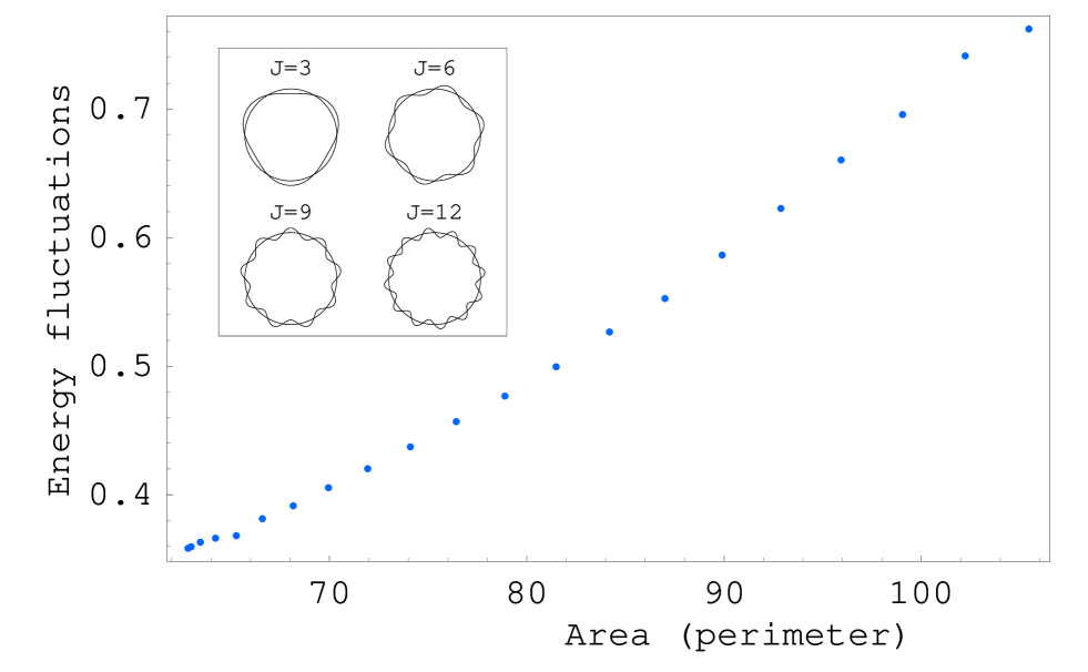
Figure 1: Energy fluctuations in the flower geometry as a function of surface area (perimeter). The horizontal axis represents the area (perimeter in the 2-dimensional case) of the flower geometry. The points on the plot represent the numerically evaluated variance of energy fluctuations inside the flower as a function of the surface area (perimeter). The boxed diagram at the top left, illustrates how the surface area (perimeter) of the flower increases while the volume (area) remains constant.

II.2 The annulus

A somewhat more radical situation is given by an annulus geometry. We divide space into three regions. Region one is a circle of radius $R_{1}$. Region two is an annulus of radii $R_{1}$ and $R_{2}$ ($R_{2}>R_{1}$), which is concentric with the circle given earlier, and region 3 is that part of space which encloses the annulus and circle. As we increase the size of the inner radius $R_{1}$, the volume of the annulus decreases, yet its surface area increases. Therefore, when considering the energy fluctuations in the annulus, we find, remarkably, that they increase as the annulus becomes thinner. This is shown in figure 2.

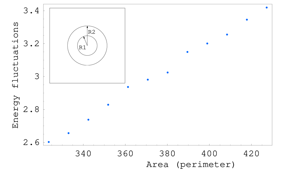
Figure 2: Magnitude of the energy fluctuations as a function of the area (perimeter: $2\pi(R_{1}+R_{2})$) of the annulus. The points on the graph show the numerically evaluated relation between the variance of the energy inside the annulus, and its surface area (perimeter). As the volume (area) of the annulus decreases, the energy fluctuations increase with the length of the perimeter.

Another property that one may consider in an annulus configuration, is the correlation between fluctuations in different regions of space. Considering the volumes $V_{1}$ and $V_{2}$ corresponding to the circle and annulus, we argue that the covariance, $\text{cov}(E^{V_{1}},E^{V_{2}})$, of the energy in these two regions is proportional to their mutual surface area (in this case the circumference of the circle).

This can be stated as a more general argument. For any two operators $O^{V_{1}}$ and $O^{V_{2}}$ defined as an integral over a density $\int_{V_{i}}\mathcal{O}d^{d}x$, $\text{cov}(O_{V_{1}},O_{V_{2}})$ scales linearly with the mutual surface area, if the the two point function $F(r=|{\vec{r}}_{1}-{\vec{r}}_{2}|)\equiv\langle 0|O({\vec{r}}_{1})O({\vec{r}}_{2})|0\rangle=\nabla^{2}g(r)$ is derived from a function $g(r)$ which has short range and is not too divergent ar $r=0$.

We give here an outline of the proof, whose details will be presented elsewhere tbp . We observe that the covariance of these operators may be written as

$$\text{cov}(O_{V_{1}},O_{V_{2}}) =\int_{V_{1}}\int_{V_{2}}\langle 0|\mathcal{O}(\vec{r}_{1})\mathcal{O}(\vec{r}_{2})|0\rangle d^{d}r_{1}\,d^{d}r_{2}$$

$$=\int_{V_{1}}\int_{V_{2}}F(|\vec{r}_{1}-\vec{r}_{2}|)d^{d}r_{1}\,d^{d}r_{2}$$

$$=\int D_{V_{1},V_{2}}(\xi)F(\xi)d\xi.$$

All information on the geometry is contained in the function

$$D_{V_{1},V_{2}}(\xi)=\int_{V_{1}}\int_{V_{2}}\delta(\xi-|\vec{r}_{1}-\vec{r}_{2}|)d^{d}r_{1}d^{d}r_{2}.$$ (1)

Using $F=\nabla^{2}g$, integrating by parts, and using the short range behavior of $g$, one can show that the covariance of the two operators scales, to leading order, as $\tilde{D}(0)=\frac{d}{d\xi}\left(\frac{D(\xi)}{\xi^{d-1}}\right)\Big{|}_{\xi=0}$ holmin .

We shall evaluate $\tilde{D}(\xi)$ for small $\xi$, where the volumes $V_{1}$ and $V_{2}$ are just touching (from the outside) at a boundary $B$. Let $\vec{r_{i}}\in V_{i}$, and consider the vectors $\vec{R}=\frac{\vec{r}_{1}+\vec{r}_{2}}{2}$, and $\vec{r}=\vec{r}_{2}-\vec{r}_{1}$. Geometrically $\vec{r}$ points from $\vec{r}_{1}$ to $\vec{r}_{2}$, and $\vec{R}$ points to the center of $\vec{r}$ (See figure 3). We may now do the integration in (1) in the $R$–$r$ coordinate system. For a given value of $\xi$, we have $|\vec{r}|=\xi$, implying that $\vec{r}_{1}$ and $\vec{r}_{2}$ are located such that the distance between them is $\xi$. Since they are located at different ends of the boundary, the vector $\vec{R}$ covers a volume of $S(B)\xi$ (where $S(B)$ is the surface area of $B$), centered at the boundary between the two regions (See figure 4). Therefore, the integration over the $R$ coordinate in (1) will give $S(B)\xi$. The integral over the radial part of the $r$ coordinate and the delta function will yield a $\xi^{d-1}$ term, and the angular part, which is restricted as $R$ gets near the boundary, will contribute a geometric factor $G_{S}$. Hence $\tilde{D}(0)=G_{S}S(B)$.

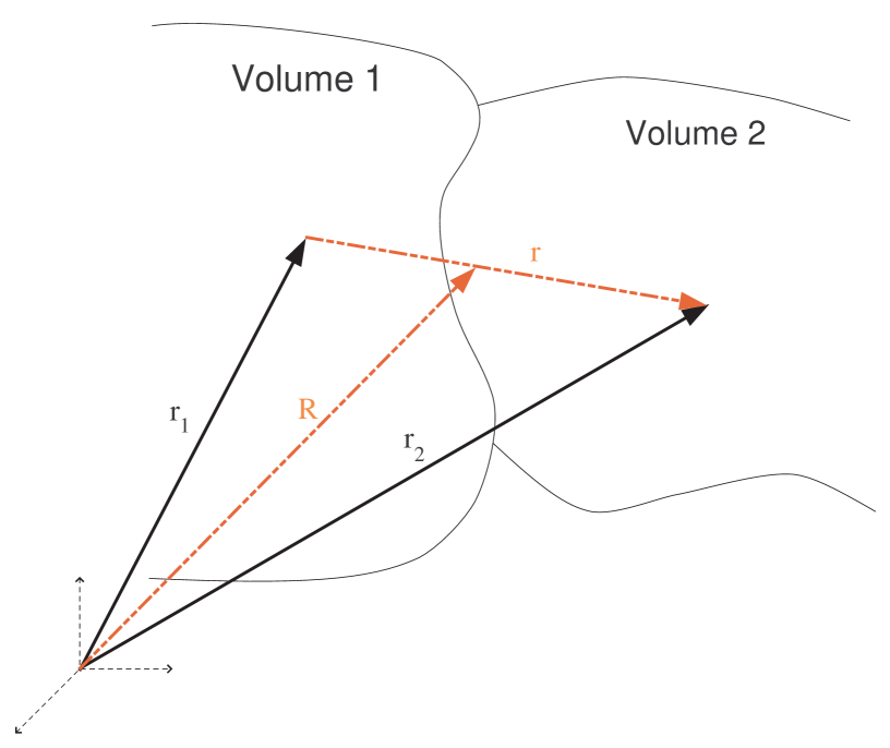
Figure 3: Geometry of the $r_{1}$–$r_{2}$ coordinate system, and the $R$–$r$ coordinate system, when $V_{1}$ and $V_{2}$ have a mutual boundary but no mutual interior.

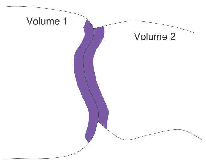
Figure 4: The region of integration in the $R$–$r$ coordinate system when $V_{1}$ and $V_{2}$ have a mutual boundary but no mutual interior.

Therefore the fluctuations in the ring and the fluctuations in the circle will be correlated such that their covariance is proportional to their mutual surface area.

III Correlations of fluctuations

We wish to generalize the above argument and show that the covariance of any two operators $O_{V_{1}}$ and $O_{V_{2}}$ will be proportional to the mutual surface area of the volumes $V_{1}$ and $V_{2}$ (if, as stated earlier, the two point correlation function $F(r)$ is derived from a short range function $g(r)$ which is not too divergent ar $r=0$.) Again, we only outline the proof.

From the arguments of the previous section, it is enough to show that $\tilde{D}(0)\propto S(B)$, with $B=B(V_{1})\cap B(V_{2})$. We consider three generic cases: first we look at a specific case where the volume $V_{1}$ is contained completely (with no mutual boundaries) in $V_{2}$. We switch to the $R$–$r$ coordinate system. To leading order, the integration over the $\vec{R}$ coordinate will be proportional to the volume, except for a region of thickness $\xi$ from the boundary. To sub-leading order, there will be contributions to the surface area term from within $V_{1}$ and external to $V_{1}$. The restriction of the angular part of $\vec{r}$ inside $V_{1}$, and external to $V_{1}$ combine so that they cancel the surface term introduced from the volume integration over the $\vec{R}$ coordinate. So, in this case, there are no surface area terms in $D(\xi)$, and therefore $\tilde{D}(0)=0$.

Next we look at regions $V_{1}$ and $V_{2}$ which have boundaries overlapping only from within each other (that is $V_{1}\subseteq V_{2}$, and they have a mutual boundary). Consider $V_{3}$ which is the complement of $V_{2}$, and define $O=O_{V_{2}}+O_{V_{3}}$. By the comment made earlier, $\text{cov}(O,O_{V_{1}})=0$. This implies $\text{cov}(O_{V_{2}},O_{V_{1}})+\text{cov}(O_{V_{3}},O_{V_{1}})=0$. Since the boundaries of $V_{3}$ and $V_{2}$ are equal (by the definition of a boundary, and assuming that the whole space has no boundary), then $B\equiv B(V_{3})\cap B(V_{1})=B(V_{2})\cap B(V_{1})$. Since $V_{3}$ is external to $V_{1}$, we have from the earlier argument that $\text{cov}(O_{V_{3}},O_{V_{1}})\propto G_{S}S(B)$, implying that $\text{cov}(O_{V_{2}},O_{V_{1}})\propto-G_{S}S(B)$.

More complex geometries may now be handled by dividing $V_{1}$, (or $V_{2}$) into subvolumes which satisfy the above conditions. This is treated in detail in tbp .

Therefore, since $\tilde{D}(0)\propto S(B)$, we have that under the restrictions mentioned, $\text{cov}(O^{V_{1}}O^{V_{2}})\propto S(B)$. In what follows we give a numerical example of this and discuss its implications.

III.1 Displaced Boxes

Our final numerical example is that of relatively placed boxes. We consider a large square box ${\cal B}$ of volume $L\times L$, and inside it, a smaller square box ${\cal A}$ of volume $L/2\times L/2$. We then move the box ${\cal A}$ by an amount $\Delta x$ along one of the symmetry axes of the box ${\cal B}$ as shown in Figure 5.

In a bulk theory, we would expect that the statistical fluctuations in the energy in the box ${\cal B}$, and those in the box ${\cal A}$ be correlated only if the boxes have some mutual volume, as there is no method by which, at a given time, fluctuations in region ${\cal A}$ ‘know of’ fluctuations in region ${\cal B}$. As the boxes are contained in each other, we expect to see some correlation between fluctuations in both regions, and as the boxes move farther apart the fluctuations will become less correlated, until the regions are disjoint, at which point measurements in region ${\cal A}$ and measurements in region ${\cal B}$ are not correlated.

However, as we showed above, when considering entanglement induced fluctuations, the covariance will be zero, unless the boxes have a mutual surface area. This is shown explicitly in the numerical calculation (See Figure 5).

The apparent interference pattern when the boundaries of the boxes almost coincide is a result of U.V. effects—these attribute to the boundaries a certain fuzziness which creates an interference pattern when they almost coincide.

The correlations of the energy fluctuations in the boxes do not behave as expected from correlations induced by a bulk theory: constant when ${\cal A}$ is inside $\cal B$, and slowly decreasing to zero as $\cal A$ exits $\cal B$. Instead the energy fluctuations are uncorrelated, until the boxes have a mutual surface. Therefore, the mechanism by which fluctuations in region $\cal B$ and region $\cal A$ know of each other, must be dependent on the boundary of the regions.

Also, the sign of the covariance changes when the surface is ‘common’ or ‘anti-common’: apart from the energies being correlated as the boundaries are in contact, we note that when the boundaries are common from within we get that a positive fluctuation in region ${\cal A}$ corresponds to a positive fluctuation in region ${\cal B}$, whereas when the boundaries are common from the outside, a positive fluctuation in ${\cal B}$ corresponds to a negative fluctuation in ${\cal A}$. This again, is an indication that the fluctuations occur on the boundary.

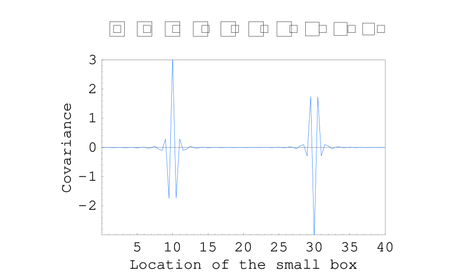
Figure 5: Correlation between energies inside the boxes, as a function of the relative position of the boxes. Note the interference pattern as the distance between the surfaces becomes of the order of the U.V. cutoff.

IV Summary

We have given several examples of area scaling of energy fluctuations in various geometries. The area fluctuations are originally calculated in a bulk - type setting, yet they have properties which are typical in boundary theories, suggesting that perhaps some corresponding boundary theory may give similar results.

In the flower geometry, we have seen that the energy fluctuations are very sensitive to the geometry of the boundary they are being measured in. Had the fluctuations been those of a canonical statistical ensemble, one would have expected that the fluctuations of the energy be proportional to the volume of the system, which in this case is constant.

In the annulus example the energy fluctuations in the annulus increase with decreasing annulus volume (area) (but increasing surface area (perimeter)). This, again, is in contradiction with our usual understanding of bulk - type theories.

Finally, when considering the energy fluctuations in two different regions of space, we have shown that these are correlated only if the regions have a mutual boundary. Moreover, the sign of the covariance changes as the boundaries are common or anti-common, which, as explained earlier, is characteristic of a boundary theory.

The surface dependence of fluctuations of extensive quantities restricted to spatial sub-volumes is a characteristic feature of glass-like statistical systems. In this paper we have discussed some implications of this behaviour in the context of a free quantum field theory in Minkowski space. Those conclusions could be also of interest in the context of primordial cosmological density fluctuations at the time of recombination, which share the same glass-like character Oaknin:2003dc .

V Acknowledgements

Research supported in part by the Israel Science Foundation under grant no. 174/00-2 and by the NSF under grant no.PHY-99-07949. A. Y. is partially supported by the Kreitman foundation. D. O is partially supported by NSERC of Canada. R. B. thanks the KITP, UC at Santa Barbara, where this work has been completed. We would like to thank B. Kol for discussions and B. Reznik for clarifying some issues regarding entanglement and the vacuum.

Appendix A Numerical calculations

For the numerical calculations we have considered a free scalar field theory in 2+1 dimensional Minkowski space. We impose an I.R. cutoff by defining all of space to have size $L\times L$ (with periodic boundary conditions), and a U.V. momentum cutoff $\frac{2\pi N}{L}$. The fields may be expanded in fourier modes:

$$\Phi(\vec{x}) =\sum_{n_{1},n_{2}=-N}^{+N}\frac{1}{L}q_{(n_{1},n_{2})}exp\left(+2\pi\imath(\sum_{j=1}^{2}n_{j}x_{j})/L\right)$$

$$\Pi^{*}(\vec{x}) =\sum_{n_{1},n_{2}=-N}^{+N}\frac{1}{L}p^{*}_{(n_{1},n_{2})}exp\left(-2\pi\imath(\sum_{j=1}^{2}n_{j}x_{j})/L\right).$$

So that

$$E_{V}=\sum_{{\vec{n}},{\vec{m}}}\left(p^{*}_{\vec{n}}p_{\vec{m}}+\kappa^{2}_{{\vec{n}}\cdot{\vec{m}}}q^{*}_{\vec{n}}q_{\vec{m}}\right)A_{V}({\vec{n}}-{\vec{m}},L),$$

where

$$\kappa^{2}_{{\vec{n}}\cdot{\vec{m}}} =\left(\frac{2\pi}{L}\right)^{2}({\vec{n}}\cdot{\vec{m}})+M^{2}$$

and

$$A_{V}({\vec{k}},L) =\frac{1}{L^{2}}\int_{V}d^{2}{\vec{x}}\,exp\left(-2\pi\imath{\vec{k}}\cdot{\vec{x}}/L\right).$$

Using the divergence theorem, one can simplify $A_{V}$

$$A_{V}({\vec{k}},L)\equiv A_{\partial V}({\vec{k}},L)=\frac{1}{L^{2}}\int_{\partial V}\hskip 3.61371pt\frac{iL}{2\pi}e^{-(2\pi\imath{\vec{k}}\cdot{\vec{x}}/L)}\frac{{\vec{k}}\cdot d{\vec{A}}}{|{\vec{k}}^{2}|}.$$ (2)

The expectation value of $E_{V_{1}}E_{V_{2}}$ in the vacuum can be expressed as

$$\text{var}(E_{V})=\frac{1}{4}\sum_{{\vec{n}},{\vec{m}}}\left(\frac{\kappa^{2}_{{\vec{n}}\cdot{\vec{m}}}}{\sqrt{\kappa_{\vec{n}}}\sqrt{\kappa_{\vec{m}}}}-\sqrt{\kappa_{\vec{n}}}\sqrt{\kappa_{\vec{m}}}\right)^{2}|F_{V}({\vec{n}}-{\vec{m}},L)|^{2},$$

and that

$$\text{cov}(E_{V_{1}},E_{V_{2}})=\frac{1}{4}\sum_{{\vec{n}},{\vec{m}}}\left(\frac{\kappa^{2}_{{\vec{n}}\cdot{\vec{m}}}}{\sqrt{\kappa_{\vec{n}}}\sqrt{\kappa_{\vec{m}}}}-\sqrt{\kappa_{\vec{n}}}\sqrt{\kappa_{\vec{m}}}\right)^{2}\times(F_{V1}({\vec{n}}-{\vec{m}},L))^{*}(F_{V2}({\vec{n}}-{\vec{m}},L)),$$

where we have defined $\kappa^{2}_{\vec{n}}=\kappa^{2}_{\vec{n}\cdot\vec{n}}$. This expression shows that the covariance is obtained as an interference process between many different modes.

For the flower geometry we have used an I.R. cutoff of L=100 units, and a U.V. cutoff of N=25, yielding $\frac{L}{2\pi N}\sim 0.6$ units. As the distance between the petals decreases to the order of the U.V. cutoff, one observes some slight deviation from the area scaling law described above. A numerical calculation of the flower geometry was carried out for free fields of masses $M=0,0.5,1$ units^-1. The graph that we have presented in Fig. 1 corresponds to $\Delta R=1$ unit, and $R=10$ units. We have also checked the results for free fields of masses $M=0,0.5,1,2.5$ units^-1, radii R=10,20 and 40 units and $\Delta R$ = 1,2, and 4 units. Apart from the deviations at large radii which, as suggested earlier, are perhaps related to “perimeter corrections”, the results were similar.

The infrared cutoff for the annulus was fixed at L=100 units of length and the ultraviolet cutoff by $\frac{L}{2\pi N}\simeq 1$ unit of length. The scalar field was taken to be massless. For the plot given in Fig. 2 we used an external radius of 40 units, and varied the inner radius from 11.5 units to 25.5 units.

For the relative boxes we have imposed an I.R. cutoff of L=100 units, and a U.V. cutoff using N=30, yielding $\frac{L}{2\pi N}\sim 1.8$ units. Box ${\cal B}$ had a boundary located at $(-20,20)\times(-20,20)$, and the smaller box’s boundary was at $(-10+\Delta x,10+\Delta x)\times(-10,10)$. Figure 5 was plotted for a field of mass $M=0.5$ units^-1. We get similar results for a higher mass field ($M=3.5$ units^-1).

References

- (1) J. D. Bekenstein, Phys. Rev. D 7, 2333 (1973).
- (2) S. W. Hawking, Commun. Math. Phys. 43, 199 (1975).
- (3) L. Susskind, J. Math. Phys. 36 (1995) 6377.
- (4) G. ’t Hooft, Abdus Salam Festschrift: a collection of talks, eds. A. Ali, J. Ellis and S. Randjbar-Daemi (World Scientific, Singapore, 1993),gr-qc/9321026
- (5) R. Bousso, Rev. Mod. Phys. 74, 825 (2002).
- (6) O. Aharony, S. S. Gubser, J. M. Maldacena, H. Ooguri and Y. Oz, Phys. Rept. 323, 183 (2000).
- (7) R. Brustein and A. Yarom, “Holographic dimensional reduction from entanglement in Minkowski space,” arXiv:hep-th/0302186.
- (8) See for example, R. P. Feynman, Statistical mechanics : a set of lectures, Reading. Mass., 1972.
- (9) L. Bombelli, R. K. Koul, J. H. Lee and R. D. Sorkin, Phys. Rev. D 34, 373 (1986).
- (10) M. Srednicki, Phys. Rev. Lett. 71, 666 (1993).
- (11) D. H. Oaknin, “Spatial correlations of energy density fluctuations in the fundamental state of the universe,” arXiv:hep-th/0305068.
- (12) R. Brustein and A. Yarom, to appear.
- (13) R. Brustein, D. Eichler, S. Foffa and D. H. Oaknin, Phys. Rev. D 65, 105013 (2002).