On plane wave and vortex-like solutions of noncommutative Maxwell-Chern-Simons theory

Abstract:

We investigate the spectrum of the gauge theory with Chern-Simons term on the noncommutative plane, a modification of the description of the Quantum Hall fluid recently proposed by Susskind. We find a series of the noncommutative massive “plane wave” solutions with polarization dependent on the magnitude of the wave-vector. The mass of each branch is fixed by the quantization condition imposed on the coefficient of the noncommutative Chern-Simons term. For the radially symmetric ansatz a vortex-like solution is found and investigated. We derive a nonlinear difference equation describing these solutions and we find their asymptotic form. These excitations should be relevant in describing the Quantum Hall transitions between plateaus and the end transition to the Hall Insulator.

1 Introduction

Since their reappearance as the effective low-energy descriptions of some string theory configurations [1] noncommutative (NC) field theories have been a subject of much attention [2]. Among the flurry of activities devoted to their study there was an interesting proposal by Susskind [3] on the possible relation between NC Chern-Simons theory and the Quantum Hall (QH) effect. Following this paper there was a considerable interest in the NC versions of the Chern-Simons (CS) theory and its properties [6]–[10]. There are many indications that noncommutativity can indeed be an interesting mathematical tool for describing 2d electron gases in strong magnetic fields [10]. It would be interesting if the NC description would lead to some specific experimentally observable differentiating phenomena.

One of the most useful tools for studying the low energy properties of the QH systems are effective lagrangians. It has been known for some time that depending on location on the quantum Hall conductivity graph the effective charge carriers differ between different plateaus and transitions on the transverse conductivity plot $\sigma_{xy}$, including the transition to the Hall insulator. It has been argued that these carriers are “particles” and “vortices” on either side of the transition and there exists an effective lagrangian describing each type of the carrier (see [4] and references therein). In two space dimensions in the presence of a perpendicular magnetic field there is a unique gauge-invariant lagrangian which is dominant in the long-wavelength limit — the Chern-Simons action. Due to this property one can assume that whatever the effective actions for particles or vortices are, they must have similar functional form in the long-wave limit, given by that of the CS. A pure CS theory can only describe the plateaus, it cannot support longitudinal conductivity. Hence as a first correction, the Maxwell term (i.e. $F^{2}$) is added, allowing for longitudinal conductivity and the possibility to describe the transition regions. It was observed by [4] that an interesting symmetry of the QH systems — the “modular group” symmetry of the complex conductivity plots could be derived just from this similarity of their effective actions for the two types of charge carriers — and it is true even beyond the linear approximation [5]. For our purposes, the essential point is that one cannot restrict oneself to just the lowest order term. In order to study the dynamics of charge carriers through the transition regions it is important to include the Maxwell term as well. In the effective action the coefficient of the Maxwell term is just $\sigma_{xx}$, which is necessary for the action of the modular group [4].

This brings us to a motivating point of our paper: if there is an effective NC theory describing the QH system, what would the noncommutativity imply for the duality? Do the effects of the order of $\theta$ (NC parameter which is $\sim 1/\rho$, $\rho$ — electron density in Susskinds proposal) spoil the resulting “modular group” action? If so, would the effect be detectable? In order to start answering these questions one first needs to find what the effective “charge carriers” for the theory in the different phases are. It therefore calls for investigation of the classical solutions of the NC Maxwell-CS theory.

In what follows we will study possible classical solutions of this action. In the next section 2 we give a short review of the NC Maxwell-CS theory and derive equations of motion for the model. In the section 3 we will find the exact solutions corresponding to the plane waves with “massive” dispersion relation. In the section 4 we will derive the nonlinear difference equation describing the static configurations that possess a non-zero vorticity and in general look like “dyons” (in the sense that there is “magnetic flux” and electric charge attached to them, “magnetic” and “electric” being just commutators of $[D_{i},D_{j}]$ and $[D_{0},D_{i}]$). We will derive some general properties of these solutions and construct some of them numerically. Some conclusions and proposals for further research are given in the end.

2 Noncommutative Chern-Simons theory

Before making any connection with the Quantum Hall effect, let us first consider noncommutative versions of the Yang-Mills — Chern-Simons theory. In this chapter we will closely follow [7, 6]. We consider the the three-dimensional noncommutative space with coordinates $x^{\mu}=(x^{0},x^{1},x^{2})$ with

$$x^{0} = t\,,\qquad[x^{1},x^{2}]=\,i\,\theta\,,\qquad\theta>0$$

$${}[t,x^{i}] = 0\,,\qquad i=(1,2)$$ (1)

which can be written as

$$[x^{\mu},x^{\nu}] = i\,\theta^{\mu\nu}$$

$$\theta^{12} = -\theta^{21}=\theta\,,\qquad\theta^{01}=\theta^{10}=0\,.$$ (2)

The noncommutative analog of the integral over all three coordinates in space time gets replaced by the mixed expression involving integral over time but trace over Fock space of the harmonic oscillator representing the spatial integral in the $(x^{1},x^{2})$ plane. Following conventions of [7], we use normalization as

$$\int\,d^{3}\,x\,\rightarrow\,\int\,dt\,(2\pi\theta)\,\mathop{\rm tr}\nolimits\,.$$ (3)

One way to introduce this noncommutativity in any 2D theory described by some action $S$ is through the so called star (${}^{\prime\prime}\star^{\prime\prime}$) product. One can show [11] that the effect of having noncommuting coordinates can be modeled by changing the multiplication rule between functions on space time. For any two functions $\phi(x)$ and $f(x)$ one has

$$\mathop{\rm tr}\nolimits\left(f({\hat{x}})\,\phi({\hat{x}})\right)\,\sim\,\int\,d^{2}x\,f({x})\,e^{\frac{i}{2}\,{\overleftarrow{\partial}}_{i}\theta^{ij}{\overrightarrow{\partial}}_{j}}\,\phi({x})\,\equiv\,\int d^{2}x\,f(x)\star\phi(x)\,,$$ (4)

where the first derivative in the exponent acts to the left and second one to the right. This product is obviously noncommutative and introduces additional nonlocality in the theory with interactions (i.e. having terms of order three or more in the action). This is because while

$$\int f(x)\star\phi(x)\,d^{2}x = \int f(x)\phi(x)\,d^{2}x\,,\qquad{\rm but}$$

$$\int f(x)\star\phi(x)\star\xi(x)\,d^{2}x \not= \int f(x)\phi(x)\xi(x)\,d^{2}x\,.$$ (5)

And therefore any action which has a term of order three or more will contain infinite number of derivatives, making the theory essentially nonlocal.

Using this formalism, it is easy to write the NC version of the CS theory

$$S=\,\frac{1}{4\pi\nu}\,\int\,dt\,d^{2}x\,\left(A_{\mu}(x)\partial_{\nu}A_{\gamma}(x)+i\frac{2}{3}A_{\mu}(x)\star A_{\nu}(x)\star A_{\gamma}(x)\right)\epsilon^{\mu\nu\gamma}\,.$$ (6)

Notice that in the commutative limit $\theta\rightarrow 0$ the non-abelian term disappears and this expression becomes the usual abelian CS action.

While this “star-product” approach proves to be very convenient in discussing the perturbation theory in this new, non-commutative field theories (see for example [12, 13]), it unfortunately hides the discreteness of this space-time picture. One essentially trades-off the Hilbert space picture of the underlying space-time to the non-locality of the action. Therefore, we will not use it in the following text, but will follow approach of [7, 6] and work directly with operators rather then with functions.

Firstly, we notice that in the NC theory described by the commutation relations (1) the derivatives with respect to the coordinates $x^{1},x^{2}$ have to be represented as operators as well:

$${\rm Since} \qquad[\partial_{i},x^{j}]=\delta_{ij}\,,\qquad{\rm and}\qquad[x^{1},x^{2}]=i\,\theta$$ (7)

$${\rm then} \qquad\partial_{1}=\frac{ix^{2}}{\theta}\,,\qquad\partial_{2}=\frac{-ix^{1}}{\theta}\,,\qquad[\partial_{1},\partial_{2}]=-\frac{i}{\theta}\,.$$

Following [7, 6], we will define the hermitean covariant derivative operators as

$$D_{\mu}=-i\partial_{\mu}+A_{\mu}(x)\,,$$ (8)

where $A_{\mu}(x)$is a generic hermitean operator representing a gauge field. Let us first write the NC CS action in these variables.

$$S=2\pi\theta\int dt\mathop{\rm tr}\nolimits\left(i{2\over 3}D_{\mu}D_{\nu}D_{\alpha}-\omega_{\mu\nu}D_{\alpha}\right)\epsilon^{\mu\nu\alpha}\,.$$ (9)

Here $\omega_{\mu\nu}$ is an antisymmetric tensor defined as follows (its spatial part is inverse of $\theta^{\mu\nu}$)

$$\omega_{12}=-\omega_{21}=-\frac{1}{\theta},\qquad\omega_{01}=\omega_{02}=0\,.$$ (10)

The cubic term in this action will produce (upon expansion in $A_{\mu}$’s and $\partial_{\nu}$) the term proportional to $A^{3}$, the quadratic term $\sim A\,\partial\,A$ and a linear term, given by

$$\sim\,-2i\,\partial_{i}\,\partial_{j}\,D_{0}\epsilon^{ij0}\,=-2i\,[\partial_{1},\partial_{2}]\,D_{0}=-\frac{2}{\theta}\,D_{0}\,.$$ (11)

This last term is, of course, the “one dimensional” CS term and is absent in the commutative theory ($\sim 1/\theta$). It has to be subtracted precisely by the linear term of the equation (9). This condition also fixes the relative sign between these two terms. For our purposes it is more convenient to introduce holomorphic and anti-holomorphic combinations as

$$D=\frac{D_{1}+i\,D_{2}}{\sqrt{2}}\qquad{\bar{D}}=\frac{D_{1}-i\,D_{2}}{\sqrt{2}i}\,.$$ (12)

Since $D_{\mu}$’s are hermitean ${\bar{D}}=D^{\dagger}$. With this definition of $D,\bar{D}$ we get

$$S=\lambda\,2\pi\theta\int dt\mathop{\rm tr}\nolimits\left(-2\,[D,\bar{D}]D_{0}+\frac{2}{\theta}D_{0}\right).$$ (13)

In order to make the following calculations easier, it is convenient to switch to the dimensionless version of operators $D,\bar{D}$ and $D_{0}$ by re-scaling them as

$$\ D\,\rightarrow\,\frac{D}{\sqrt{\theta}}\,,\qquad{\bar{D}}\,\rightarrow\,\frac{{\bar{D}}}{\sqrt{\theta}}\qquad D_{0}\,\rightarrow\,\frac{D_{0}}{\sqrt{\theta}}\,.$$ (14)

The re-scaling of $D_{0}$ also implies that $dt\rightarrow\sqrt{\theta d}{\tilde{t}}$ and new “time” is dimension-less as well. Therefore, the final form of the CS action that we are going to work with reads

$$S=\frac{2\,\lambda}{\theta^{\frac{3}{2}}}\,(2\pi\theta^{\frac{3}{2}})\int d{\tilde{t}}\mathop{\rm tr}\nolimits\left(-[D,\bar{D}]+1\right)\,D_{0}\,.$$ (15)

Now let us briefly turn to the gauge theory action. In terms of the $D,{\bar{D}}$ and $D_{0}$ operators before re-scaling the standard YM action is

$$S_{\rm YM} = \int dtd^{2}x\,\frac{1}{4g^{2}}\,F_{\mu\nu}\,F^{\mu\nu}=\int dt\,d^{2}x\,\frac{1}{4g^{2}}\,[D_{\mu},D_{\nu}][D^{\mu},D^{\nu}]$$ (16)

$$= \int dt\,d^{2}x\,\frac{1}{4g^{2}}\left(-2[D_{0},D_{i}][D_{0},D_{i}]+[D_{i},D_{j}][D_{i},D_{j}]\right)$$

$$= (2\pi\theta)\int dt\mathop{\rm tr}\nolimits\frac{1}{4g^{2}}\left(-4[D_{0},D][D_{0},{\bar{D}}]-2[D,{\bar{D}}][D,{\bar{D}}]\right).$$

After performing (14) the final form on the action is

$$S_{\rm YM}=(2\pi\theta^{\frac{3}{2}})\int d{\tilde{t}}\mathop{\rm tr}\nolimits\frac{-2}{4g^{2}\,\theta^{2}}\left(2[D_{0},D][D_{0},{\bar{D}}]+[D,{\bar{D}}][D,{\bar{D}}]\right).$$ (17)

We kept the factor $(2\pi\theta^{{3}/{2}})$ separate from the rest of the expressions (15) and (17) since it does not contribute to the relative coefficient between two different actions which will become important later. Let us now consider the total expression

$$(2\pi\theta^{\frac{3}{2}})\int d{\tilde{t}}\mathop{\rm tr}\nolimits\left\{\,\frac{-2}{4g^{2}\,\theta^{2}}\left(2[D_{0},D][D_{0},{\bar{D}}]+[D,{\bar{D}}][D,{\bar{D}}]\right)+\frac{2\,\lambda}{\theta^{3/2}}\,\left(-[D,\bar{D}]+1\right)\,D_{0}\right\}.$$

What is important is just the relative factor between the two actions, so it makes sense to express this as

$$\frac{(2\pi\theta^{3/2})}{2g^{2}\,\theta^{2}}\int_{\tilde{t}}\mathop{\rm tr}\nolimits\left\{\left(-2[D_{0},D][D_{0},{\bar{D}}]-[D,{\bar{D}}][D,{\bar{D}}]\right)+{2\tilde{\lambda}}\,\left(-[D,\bar{D}]+1\right)\,D_{0}\right\},$$ (18)

where

$$\tilde{\lambda}=2\,g^{2}\,\theta^{1/2}\,\lambda\,.$$ (19)

This is the final form of the action we are going to work with. It what follows, we can treat $D,\bar{D}$ and $D_{0}$ as independent variables, since in the non-commutative space gauge fields are operators in the same Hilbert space as the original $\partial_{i}$’s. Varying (18) with respect to $D_{0}$ one gets

$$-[D,[D_{0},{\bar{D}}]]-[{\bar{D}},[D_{0},D]]={\tilde{\lambda}}([D,{\bar{D}}]-1)\,.$$ (20)

In turn, for the $\delta{\bar{D}}$ variation the equation is

$$[D_{0},[D_{0},D]]+[D,[D,\bar{D}]]={\tilde{\lambda}}[D_{0},D]\,.$$ (21)

It is well known that in the commutative version of the CS action for the non-abelian gauge field the overall coefficient on the action must be quantized due to the topology of the $\mathop{\rm SU}\nolimits(N)$. It so happens that a similar effect takes place in the noncommutative version as well, where the effective non-abelian nature of the fields is due to the space noncommutativity. As it was shown in [7], the condition is:

$$4\pi\lambda=n\,,\qquad n\in Z-\{0\}\,.$$ (22)

3 Noncommutative plane waves

Let us now describe the plane wave solutions of the theory. Generic form of the equations of motion is given by

$$-{\ddot{D}}+[D[D,D^{\dagger}]] = -i\,\lambda\,\dot{D}$$ (23)

$$i\,[D,{\dot{D}}^{\dagger}]+i\,[D^{\dagger},\dot{D}] = \lambda[D,D^{\dagger}]-\lambda$$ (24)

(to simplify notation we use $\lambda$ instead of $\tilde{\lambda}$ in what follows). The “vacuum” solution is given by $D=a$, $D^{\dagger}=a^{\dagger}$, where $[a,a^{\dagger}]=1$ — standard creation and annihilation operators for the harmonic oscillator. Let us look for the solution of the equations (23) and (24) using the following ansatz:

$$D=a+e^{i\,\omega\,t}R_{1}\left(k\,a+k^{*}\,a^{\dagger}\right)+e^{-i\,\omega\,t}R_{2}\left(k\,a+k^{*}\,a^{\dagger}\right),$$ (25)

where $k,k^{*}$ are complex numbers and $R_{1}(x)$ and $R_{2}(x)$ are some (possibly complex) functions of the argument that can be expanded in series. Using the property that

$$\left[R_{i}\left(k\,a+k^{*}\,a^{\dagger}\right),a^{\dagger}\right]=\left[x,a^{\dagger}\right]\,\left.\frac{\partial R_{i}(x)}{\partial x}\right|_{x=k\,a+k^{*}\,a^{\dagger}}\!=\,\,k\,R_{i}^{{}^{\prime}}(k\,a+k^{*}\,a^{\dagger})$$ (26)

(which is valid only if $k$ and $k^{*}$ are c-numbers) the equation (23) can be brought to the following form:

$$\omega^{2}\,R_{1}+(k^{*})^{2}\,{R^{*}}^{{}^{\prime\prime}}_{2}+{|k|}^{2}\,R_{1}^{{}^{\prime\prime}} = \omega\,\lambda\,R_{1}$$

$$\omega^{2}\,R_{2}+(k^{*})^{2}\,{R^{*}}^{{}^{\prime\prime}}_{1}+{|k|}^{2}\,R_{2}^{{}^{\prime\prime}} = -\omega\,\lambda\,R_{2}\,.$$ (27)

At this point it is possible to assume that

$$R_{1}^{{}^{\prime\prime}}=-R_{1}\,,\qquad R_{2}^{{}^{\prime\prime}}=-R_{2}\,,\qquad R_{1,2}\sim A_{1,2}\,e^{ix}+B_{1,2}e^{-ix}$$ (28)

(an interesting case where $R^{{}^{\prime\prime}}_{1,2}=+R_{1,2}$ will be considered later). This reduces the system to

$$\omega^{2}\,R_{1}-(k^{*})^{2}\,{R^{*}}_{2}-{|k|}^{2}\,R_{1} = \omega\,\lambda\,R_{1}$$

$$\omega^{2}\,R_{2}-(k^{*})^{2}\,{R^{*}}_{1}-{|k|}^{2}\,R_{2} = -\omega\,\lambda\,R_{2}\,.$$ (29)

Taking the complex conjugate of the second equation the resulting system can be then written in matrix form

$$\pmatrix{\omega^{2}-{|k|}^{2}-\omega\,\lambda&-(k^{*})^{2}\cr-(k)^{2}&\omega^{2}-{|k|}^{2}+\omega\,\lambda}\pmatrix{R_{1}\cr{R^{*}}_{2}}=0\,.$$ (30)

The existence of the nontrivial solution for $R_{i}$ will require that determinant of the matrix on the left-hand side of (30) is zero, which in turn produces the following dispersion relation

$$\omega^{2}(\omega^{2}-\lambda^{2}-2|k|^{2})=0\,.$$ (31)

The solution $\omega=0$ is actually trivial — it is just a gauge transformation. Indeed, for this branch one has that

$$R_{2} = -\frac{k}{k^{*}}R_{1}^{*}\,,\qquad D=a+R_{1}\left(ka+k^{*}a^{\dagger}\right)-\frac{k}{k^{*}}R_{1}^{*}\left(ka+k^{*}a^{\dagger}\right)$$

$$D = U^{\dagger}\,a\,U,\ \ U^{\dagger}=U^{-1}\,,\qquad U=\left.\exp\left({\frac{1}{k^{*}}\int R_{1}(x)-\frac{1}{k}\int R_{1}^{*}(x)}\right)\right|_{x=ka+k^{*}a^{\dagger}}\,.$$ (32)

For the $\omega\neq 0$ solution one then has the “massive” modes, given by

$$\omega=\pm\sqrt{\lambda^{2}+2|k|^{2}}\,.$$ (33)

Finding the eigenvectors of the equation of the matrix in (30) corresponding to these eigenvalues gives

$$R^{*}_{2} = \left(\frac{\omega-\lambda}{\omega+\lambda}\right)\,e^{2i\,\phi}\,R_{1}$$

$$k = |k|\,e^{i\,\phi}\,,\qquad\omega^{2}=\lambda^{2}+2|k|^{2}\,.$$ (34)

However, this solution only satisfies equation (23) so far. One has to check that it is going to be compatible with equation (24) as well. Quite remarkably, upon substituting ansatz (25), this equation reduces to the derivative of condition (34).

$$R^{*^{\prime}}_{2}=\left(\frac{\omega-\lambda}{\omega+\lambda}\right)\,e^{2i\,\phi}\,R_{1}^{{}^{\prime}}\,.$$ (35)

Thus (34) is a solution. While it is not surprising that the dispersion relation is massive (the same as in the commutative YM-CS theory [14]), it shows some interesting properties — unlike the usual (i.e. commutative) plane waves there is a dependence of the polarization on the magnitude of the wave vector, $k$ (see [12] for the noncommutative QED case). In the commutative but non-abelian case the plane wave solutions will only exist for a fixed direction in the color space. Noncommutativity, a space-time feature here, will make the abelian theory effectively non-abelian, thus translating this property from the “color” space to the polarization of the waves.

Finally, let us consider the $R^{{}^{\prime\prime}}_{1,2}=+R_{1,2}$ choice. It causes a sign change for all the $k^{2}$ terms in the equations starting from (27) and leads to the following expressions:

$$\omega=\pm\sqrt{\lambda^{2}-2|k|^{2}},\ k<{\lambda\over\sqrt{2}}\,,\qquad R^{*}_{2}=-\left(\frac{\omega-\lambda}{\omega+\lambda}\right)\,e^{2i\,\phi}\,R_{1}\,,\qquad R_{1,2}\sim A_{1,2}e^{x}+B_{1,2}e^{-x}\,.$$

These solutions are not normalizable and represent excitations that are “glued” to the boundary and presumably only make sense for the finite size droplet.

4 Static gauge solutions

In this section we will look for vortex type solutions taking the “static” gauge ansatz, defined by the following condition:

$$D_{t}=\phi(N)\,,$$

where $N$ is the number operator, and $\phi$ is a well defined function of $N$. Such functions are essentially defined through the spectral representation (see for example Reed and Simon). All fields are taken to be independent of the temporal coordinate, hence $\partial_{t}$ effectively vanishes. The corresponding ansatz for the spatial part is given by

$$D=f(N)a\qquad D^{\dagger}=a^{\dagger}f^{\dagger}(N)\,.$$

In the computations that follow we use the following identities which can be established using the spectral representation, for example:

$$[a,g(N)] = a(g(N)-g(N-1))=(g(N+1)-g(N))a$$

$${}[a^{\dagger},g(N)] = -a^{\dagger}(g(N+1)-g(N))=(g(N)-g(N-1))a^{\dagger}\,.$$

Before proceeding to the equations of motion, there are two expressions that are useful to compute. One is the “magnetic field” $B(N)=[D,D^{\dagger}]$ while the other is $E=[D_{t},D]$ which corresponds to the holomorphic component of the “electric” field. We find

$$B(N)=(N+1)f^{\dagger}(N)f(N)-Nf^{\dagger}(N-1)f(N-1)$$ (36)

while

$$E=-f(N)(\phi(N+1)-\phi(N))a\,.$$ (37)

If for the solution neither of these changes then it is just the gauge transformation as discussed in the previous section ($\omega=0$ modes).

Now let us proceed to the equations (23) and (24) in terms of these variables. The Ampère law becomes

$$\left[D_{t},\left[D_{t},D\right]\right]+\left[D,\left[D,D^{\dagger}\right]\right]=\lambda[D_{t},D]$$ (38)

while the Gauss law becomes

$$-\left[D^{\dagger},\left[D_{t},D\right]\right]-\left[D,\left[D_{t},D^{\dagger}\right]\right]=\lambda(\left[D,D^{\dagger}\right]+1)\,.$$ (39)

Using definition

$$Q(N)=\phi(N)-\phi(N+1)$$

we get the following operator equations for (38) and (39) the Ampère law and the Gauss law, respectively,

$$f(N)(Q(N))^{2}a+f(N)(B(N+1)-B(N))a = \lambda f(N)Q(N)a\qquad$$ (40)

$$2\left((N+1)f^{\dagger}(N)f(N)Q(N)-Nf^{\dagger}(N-1)f(N-1)Q(N-1))\right) = \lambda(B(N)-1)\,.$$ (41)

The Ampere law, equation (40) can be simplified further by multiplying on the right by $a^{\dagger}$. This yields the operator $N+1$ as a common, positive, right multiplying factor in each term, which we can then remove, since it never vanishes. Similarly the function $f(N)$ appears as a left multiplying factor in each term. With the hypothesis that $f(N)$ never vanishes, we can also remove it giving the equation

$$Q(N)^{2}+(N+2)f^{\dagger}(N+1)f(N+1)-2(N+1)f^{\dagger}(N)f(N)+Nf^{\dagger}(N-1)f(N-1)=\!-\lambda Q(N)$$

which can be written as

$$\frac{1}{4}(2Q(N)-\lambda)^{2}+\nabla^{2}\left((N+1)f^{\dagger}(N)f(N)\right)=\frac{\lambda^{2}}{4}\,,$$ (42)

where $\nabla^{2}$ is the appropriate discrete laplacian operator. The Gauss law, equation (41) can be re-written as

$$(N+1)\left(2Q(N)-\lambda\right)f^{\dagger}(N)f(N)-N(2Q(N-1)-\lambda)f^{\dagger}(N-1)f(N-1)=-\lambda\,.$$

This equation can actually be solved as an operator equation, easily seen by using the spectral representation, to give

$$(2Q(N)-\lambda)f^{\dagger}(N)f(N)=-\lambda\,..$$ (43)

Replacing for $(2Q(N)-\lambda)$ in equation (42) yields

$${1\over 4}\left({\lambda\over f^{\dagger}(N)f(N)}\right)^{2}+\nabla^{2}\Big{(}(N+1)f^{\dagger}(N)f(N)\Big{)}={\lambda^{2}\over 4}\,.$$ (44)

Defining $u(N)=(N+1)f^{\dagger}(N)f(N)$ and $g^{2}=\lambda^{2}/4$ we get the nonlinear recurrence relation (in the spectral representation)

$$u_{n+1}-2u_{n}+u_{n-1}+g^{2}\left({n+1}\over u_{n}\right)^{2}=g^{2}\,.$$ (45)

$u_{-1}$ is taken to be zero as can be seen from consistency with its definition. Hence specifying the value of $u_{0}$ is sufficient to determine all subsequent values of $u_{n}$ for $n\geq 1$.

Let us study the simplest solution of our system of equations (43) and (44). One obvious possibility is to take $Q(N)=0$ and $f^{\dagger}(N)f(N)=1$ since the (discrete) laplacian of $N+1$ evidently vanishes. This corresponds to the “vacuum” solution of the quantum Hall system of Susskind and its gauge transformations. The “magnetic field” given by (36) is $[D,D^{\dagger}]=1$ and the energy ${\cal E}\sim\mathop{\rm Tr}\nolimits(B^{2}-1)=0$. The quasi-hole/particle excitation that are found in the pure Chern-Simons theory of Susskind are actually absent in this theory. Indeed, it seems that the vacuum solution is unstable due to the addition of the Yang-Mills term.

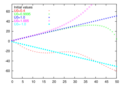
Figure 1: Behavior of the solutions of the equation (45) for the different values of $u_{0}$. The plot shows $u_{n}$ for $n$ between 0 and 50.

Numerical analysis of the recurrence relation (45) yields the following intriguing behavior, some of which is shown on figure 1. It turns out that the type of solution one gets greatly depends on the initial value $u_{0}$. If $u_{0}$ is taken to be one, we get the above mentioned vacuum solution (data with $u_{0}=1.0$). However if $u_{0}$ is perturbed even slightly greater than one, the recurrence relation is dominated by the right hand side and values for subsequent $u_{n}$ become large (data with $u_{0}=1.005$). When this is the case, the nonlinear term on the left hand side becomes negligible, yielding a simple recurrence relation

$$u_{n+1}-2u_{n}+u_{n-1}=g^{2}$$ (46)

with solution

$$u_{n}\sim g^{2}\frac{n(n+1)}{2}\,.$$

This solution is asymptotic to the solution found by [15] for the Yang-Mills-Chern-Simons theory with the pure $D^{3}$ expression for the Chern-Simons term. If $u_{0}$ is perturbed slightly less than one, the behavior is very interesting but always pathological. It can essentially only be analyzed numerically and we find that it is possible that the solution for $u_{n}$ oscillates about a straight line of slope $-1$ (data for $u_{0}=0.4$ and $u_{0}=-1.0$). For certain discrete set of initial values, the value of $u_{n},n=1,2,3,\dots$ etc. becomes exactly zero (close to data for $u_{0}=0.9995$). Such initial values are singular as the recurrence relation becomes ill defined. However, even generic initial starting points $0<u(0)<1$ are also pathological since eventually the recurrence relation drives $u_{n}<0$ for $n$ sufficiently large, as we will prove in the next section. This is unphysical since $u_{n}$ represents a positive semi-definite operator.

5 Asymptotic solutions

Let us now discuss some of the properties of the solutions of the equation (45). First, it is useful to derive the “integral form” of this expression. One can write

$$u_{k+1}-u_{k}=u_{k}-u_{k-1}+g^{2}\left(1-\frac{(k+1)^{2}}{u_{k}^{2}}\right).$$ (47)

Let us then sum left and right sides of this equation for $k$ running from zero to some integer $n$. Two terms on the left as well as the first two terms on the right are the so-called “telescoping sum” and can easily be summed up to yield

$$u_{n+1}-u_{0}=u_{n}+g^{2}\sum_{k=0}^{k=n}\left(1-\frac{(k+1)^{2}}{u_{k}^{2}}\right).$$ (48)

Moving $u_{0}$ to the right hand side and $u_{n}$ to the left, one can repeat the summation again for $n$ going from $0$ to some other integer $(l-1)$, producing the following formula for generic $u_{l}$

$$u_{l}=u_{0}(l+1)+g^{2}\frac{l(l+1)}{2}-g^{2}\sum_{n=0}^{n=l-1}\sum_{k=0}^{k=n}\left(\frac{(k+1)^{2}}{u_{k}^{2}}\right).$$ (49)

The whole sequence of $u_{l}$’s is therefore determined by its first term, $u_{0}$ (and $\lambda^{2}$ of course). Since we are interested in the solution where $u_{l}>0$ for all $l>=0$, we will therefore consider what happens only for $u_{0}>0$ as well. One special solution of this recursion relation is easy to find, i.e.

$${\rm if}\qquad u_{0}=1\qquad\forall\,g\qquad{\rm then}\qquad u_{l}=(l+1)\,.$$ (50)

For the case of $u_{0}>1$ by induction one can prove that $u_{l}>u_{0}(l+1)$. This follows immediately from the form of the equation (48) since each term in the sum on the right hand side is positive. However, one can improve this estimate by using this fact and (49), i.e.

$$u_{l} = u_{0}(l+1)+g^{2}\frac{l(l+1)}{2}-g^{2}\sum_{n=0}^{n=l-1}\sum_{k=0}^{k=n}\left(\frac{(k+1)^{2}}{u_{k}^{2}}\right)$$ (51)

$$> u_{0}(l+1)+g^{2}\frac{l(l+1)}{2}-g^{2}\sum_{n=0}^{n=l-1}\sum_{k=0}^{k=n}\left(\frac{1}{u_{0}^{2}}\right)$$

$$> u_{0}(l+1)+g^{2}\left(1-\frac{1}{u_{0}^{2}}\right)\frac{l(l+1)}{2}\,.$$

Since $u_{0}>1$ the coefficient at the $g^{2}$ term of this formula is positive and so the $u_{l}$ is growing at least quadratically with $l$. One can improve this estimate once more by noticing that since eventually $u_{l}\,\sim\,l^{2}$ one can iterate (49) one more time. The actual form of the asymptotic expression for $u_{l}$ can be found from the self-consistency condition and is

$$u_{l}=g^{2}\frac{l(l+1)}{2}+\alpha\,l+\beta\,{\rm ln}(l)+\gamma+{o}(l)\,,$$ (52)

where $\alpha,\beta$ and $\gamma$ are some functions of $\lambda$ and $u_{0}$.

Let us now turn to a case of $u_{0}<1$. Analysis of the previous paragraph has to be modified by essentially changing all ${}^{\prime\prime}>^{\prime\prime}$ signs to the ${}^{\prime\prime}<^{\prime\prime}$ ones with one extra condition that $u_{l}>0$ for all “previous” $l$’s. Indeed, assuming that $u_{k}>0\ \ \forall\,k<l$ one can use induction to prove (using (48) as before) that

$$0<u_{l}<u_{0}(l+1)\,.$$ (53)

Notice that the condition that all the previous $u_{l}$’s are positive is essential, since it is the absolute value that matters in the nonlinear part of (48) (i.e. $1/u_{l}^{2}$ ). Let us assume that up to a particular $l$ this condition is satisfied. Then, using equation (49) one has that

$$u_{l} = u_{0}(l+1)+g^{2}\frac{l(l+1)}{2}-g^{2}\sum_{n=0}^{n=l-1}\sum_{k=0}^{k=n}\left(\frac{(k+1)^{2}}{u_{k}^{2}}\right)$$ (54)

$$< u_{0}(l+1)+g^{2}\frac{l(l+1)}{2}-g^{2}\sum_{n=0}^{n=l-1}\sum_{k=0}^{k=n}\left(\frac{1}{u_{0}^{2}}\right)$$

$$< u_{0}(l+1)+g^{2}\left(1-\frac{1}{u_{0}^{2}}\right)\frac{l(l+1)}{2}\,.$$

Here the coefficient at the quadratic part is now negative, since $|u_{0}|<1$. This tells us that for sufficiently large $l$ one clearly has that

$$u_{l}<u_{0}(l+1)+g^{2}\left(1-\frac{1}{u_{0}^{2}}\right)\frac{l(l+1)}{2}<0\qquad{\rm for}\qquad l>\frac{2u_{0}^{3}}{g^{2}(1-u_{0}^{2})}$$ (55)

which clearly contradicts our assumptions. Therefore, for any $0<u_{0}<1$ the recurrence relation (45) will necessarily produce at least one negative $u_{l}$.

In view that $u$’s represent a norm for the Hilbert space states and have to be positive, it would seem then that $u_{0}<1$ is not a good starting point. However, should the total size $n$ of the Hilbert space be restricted [8] this is not so. Since the number operator $N$ eigenvalues roughly correspond to the radius squared in the plane, this limiting value would correspond to a finite size droplet. It quite possible that some of the $u_{0}$’s which are less then one would be allowed. We are currently investigating this possibility.