Pair creation of de Sitter black holes on a cosmic string background

Abstract

We analyze the quantum process in which a cosmic string breaks in a de Sitter (dS) background, and a pair of neutral or charged black holes is produced at the ends of the string. The energy to materialize and accelerate the pair comes from the positive cosmological constant and, in addition, from the string tension. The compact saddle point solutions without conical singularities (instantons) or with conical singularities (sub-maximal instantons) that describe this process are constructed through the analytical continuation of the dS C-metric. Then, we explicitly compute the pair creation rate of the process. In particular, we find the nucleation rate of a cosmic string in a dS background, and the probability that it breaks and a pair of black holes is produced. Finally we verify that, as occurs with pair production processes in other background fields, the pair creation rate of black holes is proportional to $e^{S}$, where the gravitational entropy of the black hole, $S$, is given by one quarter of the area of the horizons present in the saddle point solution that mediates the process.

I Introduction

In nature there are few known processes that allow the production of black holes. The best well-known is the gravitational collapse of a massive star or cluster of stars. Due to fermionic degeneracy pressure these black holes cannot have a mass below the Oppenheimer-Volkoff limiting mass ($\sim 3M_{\odot}$ in recent calculations). Another one is the quantum Schwinger-like process of black hole pair creation in an external field. These black holes can have Planck dimensions and thus their evolution is ruled by quantum effects. Moreover, gravitational pair creation involves topology changing processes, and allows a study of the statistical properties of black holes, namely: it favors the conjecture that the number of internal microstates of a black hole is given by the exponential of one-quarter of the area of the black hole horizon, and it gives useful clues to the black hole information paradox.

The evaluation of the black hole pair creation rate has been done at the semiclassical level using the instanton method. An instanton is an Euclidean solution that interpolates between the initial and final states of a classically forbidden transition, and is a saddle point for the Euclidean path integral that describes the pair creation rate. This instanton method has been first introduced in studies about decay of metastable termodynamical states, and it has been applied in the context of pair creation of particles and fields in the absence of gravity, by several authors (see, e.g., OscLem_FalVac for a review).

I.1 Backgrounds for black hole pair creation. Instantons

The instanton method has been also introduced as a framework for quantum gravity, with successful results in the analysis of gravitational thermodynamic issues and black hole pair production processes, among others (see EQG-book ). The regular instantons that describe the process we are interested in - the pair creation of black holes in an external field - can be obtained by analytically continuing (i) a solution found by Ernst Ernst , (ii) the de Sitter black hole solutions, (iii) a solution found by Kinnersley and Walker known as the C-metric KW , (iv) a combination of the above solutions, or (v) the domain wall solution VilenkinStringIpserSikivie . To each one of these five families of instantons corresponds a different way by which energy can be furnished in order to materialize the pair of black holes and to accelerate them apart. In case (i) the energy is provided by the electromagnetic Lorentz force, in case (ii) the strings tension furnishes this energy, in case (iii) the energy is provided by the rapid cosmological expansion associated to the positive cosmological constant $\Lambda$, in case (iv) the energy is provided by a combination of the above fields, and finally in case (v) the energy is given by the repulsive gravitational field of the domain wall. Since these solutions play a fundamental role, we will now briefly discuss some of them that are less known. The C-metric KW describes a pair of black holes (neutral or charged) uniformly accelerating in opposite directions. The solution has conical singularities at its angular poles that, when conveniently treated, can be interpreted as two strings from each one of the black holes towards the infinity and whose tension provides the necessary force to pull apart the black holes. By appending a suitable external electromagnetic field, Ernst Ernst has removed all the conical singularities of the charged flat C-metric. The Ernst solution then describes two oppositely charged black holes undergoing uniform acceleration provided by the Lorentz force associated to the external field (for the magnetic solution see Ernst , while the explicit electric solution can be found in Brown Brown ). Asymptotically, the Ernst solution reduces to the Melvin universe Melvin . The Lorentz sector of the C-metric and Ernst solution describe the evolution of the black holes after their creation. The usual de Sitter black hole solutions, when euclideanized, give also instantons for pair creation of black holes. Indeed, the de Sitter black holes solutions can be interpreted as representing a black hole pair being accelerated by the cosmological constant.

It was believed that the only black hole pairs that could be nucleated were those whose Euclidean sector was free of conical singularities (instantons). This regularity condition restricted the mass and charge of the black holes that could be produced, and physically it meant that the only black holes that could be pair produced were those that are in thermodynamic equilibrium. However, Wu WuSubMax , and Bousso and Hawking BoussoHawkSubMax have shown that Euclidean solutions with conical singularities (sub-maximal instantons) may also be used as saddle points for the pair creation process, as long as the spacelike boundary of the manifold is chosen in order to contain the conical singularity and the metric is specified there. In this way, pair creation of black holes whose horizons are not in thermodynamic equilibrium is also allowed.

I.2 Historical overview on pair creation process in an external field

We will describe the studies that have been done on pair creation of black holes in an external field.

(i) The suggestion that the pair creation of black holes could occur in quantized Einstein-Maxwell theory has been given by Gibbons Gibbons-book in 1986, who has proposed that extremal black holes could be produced in a background magnetic field and that the appropriate instanton describing the process could be obtained by euclideanizing the extremal Ernst solution. This idea has been recovered by Giddings and Garfinkle GarfGidd that confirmed the expectation of Gibbons-book and, in addition, they have constructed an Ernst instanton that describes pair creation of nonextreme black holes. The explicit calculation of the rate for this last process has lead Garfinkle, Giddings and Strominger GarfGiddStrom_Sbh to conclude that the pair creation rate of nonextreme black holes is enhanced relative to the pair creation of monopoles and extreme black holes by a factor $e^{S_{\rm bh}}$, where $S_{\rm bh}={\cal A}_{\rm bh}/4$ is the Hawking-Bekenstein entropy of the black hole and ${\cal A}_{\rm bh}$ is the area of the black hole event horizon. This issue of black hole pair creation in a background magnetic field and the above relation between the pair creation rate and the entropy has been further investigated by Dowker, Gauntlett, Kastor and Traschen DGKT , by Dowker, Gauntlett, Giddings and Horowitz DGGH , and by Ross RossU(1) , but now in the context of the low energy limit of string theory and in the context of five-dimensional Kaluza-Klein theory. To achieve their aim they have worked with an effective dilaton theory which, for particular values of the dilaton parameter, reduces to the above theories, and they have explicitly constructed the dilaton Ernst instantons that describe the process. The one-loop contribution to the magnetic black hole pair creation problem has been given by Yi YiPConeLoop . Brown Brown ; Brown2 has analyzed the pair creation of charged black holes in an electric external field. Hawking, Horowitz and Ross HawHorRoss (see also Hawking and Horowitz HawkHor ) have related the rate of pair creation of extreme black holes with the area of the acceleration horizon. In the nonextreme case, the rate has an additional contribution from the area of the black hole horizon. From these relations emerges an explanation for the fact, mentioned above, that the pair creation rate of nonextreme black holes is enhanced relative to the pair creation of extremal black holes by precisely the factor $e^{{\cal A}_{\rm bh}/4}$. For a detailed discussion concerning the reason why this factor involves only ${\cal A}_{\rm bh}$ and not two times this value see also Emparan Emparan . It has to do with the fact that the internal microstates of two members of the black hole pair are correlated.

(ii) The study of pair creation of de Sitter (dS) black holes has been also investigated. Notice that the dS black hole solution can be interpreted as a pair of dS black holes that are being accelerated apart by the positive cosmological constant. The cosmological horizon can be seen as an acceleration horizon that impedes the causal contact between the two black holes, and this analogy is perfectly identified for example when we compare the Carter-Penrose diagrams of the C-metric and of the dS Schwarzschild black hole, for example. The study on pair creation of black holes in a dS background has begun in 1989 by Mellor and Moss MelMos , who have identified the gravitational instantons that describe the process (see also Romans Rom for a detailed construction of these instantons). The explicit evaluation of the pair creation rates of neutral and charged black holes accelerated by a cosmological constant has been done by Mann and Ross MannRoss . This process has also been discussed in the context of the inflationary era undergone by the universe by Bousso and Hawking BoussoHawk . Garattini GaratinniOneLoop , and Volkov and Wipf VolkovWipf have computed the one-loop factor for this pair creation process, something that in gravity quantum level is not an easy task. Booth and Mann BooMann have analyzed the cosmological pair production of charged and rotating black holes. Pair creation of dilaton black holes in a dS background has also been discussed by Bousso BoussoDil .

(iii) In 1995, Hawking and Ross HawkRoss-string and Eardley, Horowitz, Kastor and Traschen DougHorKastTras have discussed a process in which a cosmic string breaks and a pair of black holes is produced at the ends of the string. The string tension then pulls the black holes away, and the C-metric provides the appropriate instantons to describe their creation. In order to ensure that this process is physically consistent Achúcarro, Gregory and Kuijken AchGregKui , and Gregory and Hindmarsh GregHind have shown that a conical singularity can be replaced by a Nielson-Olesen vortix. This vortix can then pierce a black hole AchGregKui , or end at it GregHind . Moreover, it has been suggested that even topologically stable strings can end at a black hole HawkRoss-string -PreskVil .

(iv) We can also consider a pair creation process, analyzed by Emparan Empar-string , involving cosmic string breaking in a background magnetic field. In this case the Lorentz force is in excess or in deficit relative to the net force necessary to furnish the right acceleration to the black holes, and this discrepancy is eliminated by the string tension. The instantons describing this process are a combination of the Ernst and C-metric intantons.

(v) The gravitational repulsive energy of a domain wall provides another mechanism for black hole pair creation. This process has been analyzed by Caldwell, Chamblin and Gibbons CaldChamGibb , and by Bousso and Chamblin BouCham in a flat background, while in an anti-de Sitter background the pair creation of topological black holes (with hyperbolic topology) has been analyzed by Mann MannAdS .

Other studies concerning the process of pair creation in a generalized background is done in Other .

I.3 Pair creation of magnetic $\bm{v}s$ electric black holes

It has been noticed that oddly the pair creation of electric black holes was apparently enhanced relative to the pair creation of magnetic black holes. This was a consequence of the fact that the Maxwell action has opposite signs in the two cases. Now, this discrepancy between the two pair creation rates was not consistent with the idea that electric and magnetic black holes should have identical quantum properties. This issue has been properly and definitively clarified by Hawking and Ross HawkRoss and by Brown Brown2 , who have shown that the magnetic and electric solutions differ not only in their actions, but also in the nature of the boundaries conditions that can be imposed on them. More precisely, one can impose the magnetic charge as a boundary condition at infinity but, in the electric case, one instead imposes the chemical potential as a boundary condition. As a consequence they proposed that the electric action should contain an extra Maxwell boundary term. This term cancels the opposite signs of the Maxwell action, and the pair creation rate of magnetic and electric black holes is equal.

I.4 Pair creation of black holes and the information loss problem

The process of black hole pair creation gives also useful clues to the discussion of the black hole information loss problem InformationLossLOSS . Due to the thermal Hawking radiation the black holes evaporate. This process implies that one of the following three scenarios occurs (see InformationLossREVIEW for reviews): (i) the information previously swallowed to the black hole is destroyed, (ii) this information is recovered to the exterior through the Hawking radiation, or (iii) the endpoint of the evaporation is a Plank scale remnant which stores the information. There are serious difficulties associated to each one of this scenarios. Scenario (i) implies non-unitarity and violation of energy conservation, scenario (ii) implies violation of locality and causality, and the main problem with scenario (iii) is that a huge energy is needed in order to store all the information that has been swallowed by the black hole, and a Planck scale remnant has very little energy. Pair creation of black holes has been used to test these scenarios. Indeed, it has been argued InformationLossREVIEW that if one demands preservation of unitarity and of locality then a careful analysis of the one-loop contribution to the pair creation process indicates that the Hawking process would leave behind a catastrophic infinite number of remnants. So the remnant hypothesis seems to be discarded, although some escape solutions can be launched InformationLossREVIEW . On the other side, Hawking, Horowitz and Ross HawHorRoss have called attention to the fact that the same instantons that describe pair creation can, when reversed in time, describe their pair annihilation, as long as the black holes have appropriate initial conditions such that they come to rest at the right critical separation (this annihilation process was also discussed by Emparan Emparan ). One can then construct HawHorRoss an argument that favors the information loss scenario: black holes previously produced as a particle-antiparticle pair can accrete information and annihilate, with their energy being given off as electromagnetic and gravitational radiation. Therefore, the information loss scenario seems to occur at least in this annihilation process.

I.5 Energy released during and after pair creation

An important process that accompanies the production of the black hole pair and the subsequent acceleration that they suffer is the emission of electromagnetic and gravitational radiation. In an asymptotically flat background, an estimate for the amount of gravitational radiation radiated during the pair creation period has been given by Cardoso, Dias and Lemos VitOscLem : $\Delta E=\frac{4Gc}{\pi}\frac{\gamma^{3}m^{3}}{\hbar}$, where $m$ is the mass of each one of the created black holes and $\gamma=(1-v^{2}/c^{2})^{-1/2}$ is the Lorentz factor. This value can lead, under appropriate numbers of $m$ and $\gamma$ to huge quantities, and is a very good candidate to emission of gravitational radiation. For example, for black holes with 30 times the Planck mass and with $10\%$ of the velocity of light, the gravitational energy released is $\Delta E\sim 10^{13}\,{\rm J}$, which is about 100 times the rest energy of the pair.

The gravitational radiative properties of the resulting accelerated black holes has been analyzed by Bičák, and Pravda and Pravdova BPP . In a dS background, the gravitational radiation emitted by uniformly accelerated sources without horizons has been analyzed by Bičák and Krtouš BicKrt , and the radiative properties of accelerated black holes have been studied by Krtouš and Podolský KrtPod .

I.6 Plan of the paper

In this paper we discuss the process in which a cosmic string nucleates in a de Sitter (dS) background, and then breaks producing a pair of black holes at its ends. Therefore, the energy to materialize and accelerate the pair comes from the positive cosmological constant and, in addition, from the string tension. This process is a combination of the processes considered in (ii) MelMos -VolkovWipf and in (iii) HawkRoss-string -GregHind . The instantons for this process can be constructed by analytically continuing the dS C-metric found by Plebański and Demiański PlebDem and analyzed by Podolský and Griffiths PodGrif2 , and in detail by Dias and Lemos OscLem_dS-C .

The plan of this paper is as follows. In Sec. II, we describe the semiclassical instanton method used to evaluate the pair creation rate. In section III we construct, from the dS C-metric, the instantons that describe the pair creation process. Then, in section IV, we explicitly evaluate the pair creation rate for each one of the cases discussed in Sec. III. In Sec. V we verify that the usual relation between pair creation rate, entropy and total area holds also for the pair creation process discussed in this paper. Finally, in Sec. VI concluding remarks are presented. In the Appendix a heuristic derivation of the pair creation rates is given. Throughout this paper we use units in which $G=c=\hbar=1$.

II Black hole pair creation rate: the instanton method

The pair creation of black holes in a de Sitter (dS) background is described, according to the no-boundary proposal of Hartle and Hawking HartleHawk , by the propagation from nothing to a 3-surface boundary $\Sigma$. The amplitude for this process is given by the wave function

$$\Psi(h_{ij},A_{i})=\int d[g_{\mu\nu}]d[A_{\mu}]e^{-I(g_{\mu\nu},A_{\mu})}\>,$$ (1)

where $h_{ij}$ and $A_{i}$ are the induced metric and electromagnetic potential on the boundary $\Sigma=\partial{\cal M}$ of a compact manifold ${\cal M}$, $d[g_{\mu\nu}]$ is a measure on the space of the metrics $g_{\mu\nu}$ and $d[A_{\mu}]$ is a measure on the space of the Maxwell field $A_{\mu}$, and $I(g_{\mu\nu},A_{\mu})$ is their Euclidean action. The path integral is over all compact metrics and potentials on manifolds ${\cal M}$ with boundary $\Sigma$, which agree with the boundary data on $\Sigma$. For a detailed discussion of the no-boundary proposal applied to the study of black hole pair creation see Bousso and Chamblin BouCham .

In the semiclassical instanton approximation, the dominant contribution to the path integral comes from metrics and Maxwell fields which are near the solutions (instantons) that extremalize the Euclidean action and satisfy the boundary conditions. Thus, considering small fluctuations around this solution, $g_{\mu\nu}\rightarrow g_{\mu\nu}+\tilde{g}_{\mu\nu}$ and $A_{\mu}\rightarrow A_{\mu}+\tilde{A}_{\mu}$, the action expands as

$$I=I_{\rm inst}(g_{\mu\nu},A_{\mu})+\delta^{2}I(\tilde{g}_{\mu\nu})+\delta^{2}I(\tilde{A}_{\mu})+\cdots\>,$$ (2)

where $\delta^{2}I$ are quadratic in $\tilde{g}_{\mu\nu}$ and $\tilde{A}_{\mu}$, and dots denote higher order terms. The wave function, that describes the creation of a black hole pair from nothing, is then given by $\Psi_{\rm inst}=Be^{-I_{\rm inst}}$, where $I_{\rm inst}$ is the classical action of the gravitational instanton that mediates the pair creation of black holes, and the prefactor $B$ is the one loop contribution from the quantum quadratic fluctuations in the fields, $\delta^{2}I$. Similarly, the wave function that describes the nucleation of a dS space with a string from nothing is $\Psi_{\rm string}\propto e^{-I_{\rm string}}$, and the wave function describing the nucleation of a dS space from nothing is $\Psi_{\rm dS}\propto e^{-I_{\rm dS}}$. The nucleation probability of the dS space from nothing, of the dS space with a string from nothing, and of a space with a pair of black holes from nothing is then given by $|\Psi_{\rm dS}|^{2}$, $|\Psi_{\rm string}|^{2}$ and $|\Psi_{\rm inst}|^{2}$, respectively.

We may now ask four questions: what is the probability for (i) pair creation of black holes in a dS spacetime, (ii) the nucleation of a string in a dS background, (iii) the process in which a string in a dS background breaks and a pair of black holes is created, and (iv) the combined process (ii)+(iii). In the process (i) the energy to materialize the pair comes only from the positive cosmological constant background, $\Lambda$. The system does not contain a string and the probability for this process has been found in MannRoss . The aim of the present paper is to compute explicitly the probability for processes (ii)-(iv). It is important to note that in the process (iii), one assumes that the initial background contains a string, i.e. , the question that is being asked is: given that the string is already present in our initial system, what is the probability that it breaks and a pair of black holes is produced and accelerated apart by $\Lambda$ and by the string tension? On the other side, in (iv) one is asking: starting from a pure dS background, what is the probability that a string nucleates on it and then breaks forming a pair of black holes? Naturally, the probability for process (iv) is the product of the probability for process (ii) and the probability for process (iii).

According to the no-boundary proposal, the nucleation rate of a string in a dS background is proportional to $|\Psi_{\rm string}|^{2}/|\Psi_{\rm dS}|^{2}$, i.e.,

$$\Gamma_{\rm string/dS}\simeq\eta\bar{\eta}\,e^{-2I_{\rm string}+2I_{\rm dS}}\>.$$ (3)

The pair creation rate of black holes when a string breaks in a dS background is given by

$$\Gamma_{\rm BHs/string}\simeq\eta\,e^{-2I_{\rm inst}+2I_{\rm string}}\>,$$ (4)

and the pair creation rate of black holes when process (iv) occurs is given by the product of (3) and (4), i.e.,

$$\Gamma_{\rm BHs/dS}\simeq\tilde{\eta}\,e^{-2I_{\rm inst}+2I_{\rm dS}}\>.$$ (5)

In Sec. IV we will find $I_{\rm inst}$ and $I_{\rm string}$. In the three relations above, $\bar{\eta}$, $\eta$ and $\tilde{\eta}$ are one-loop prefactors which will not be considered in this paper. The evaluation of this one-loop prefactor has been done only in a small number of cases, namely for the vacuum background by Gibbons, Hawking and Perry GibbHawPer , for the Schwarzschild instanton by Gross, Perry and Yaffe GrossPerryYaffe , for other asymptotically flat instantons by Young Young , for the dS background by Gibbons and Perry GibbPer and Christensen and Duff ChristDuff , for the dS-Schwarzschild instanton by Ginsparg and Perry GinsPerry , Young YoungdS , Volkov and Wipf VolkovWipf and Garattinni GaratinniOneLoop , and for the Ernst instanton by Yi YiPConeLoop .

At this point we must specify the Euclidean action needed to compute the path integral (1). This issue was analyzed and clarified in detail by Hawking and Ross HawkRoss and by Brown Brown2 . Now, due to its relevance for the present paper, we briefly discuss the main results of HawkRoss ; Brown2 . One wants to use an action for which it is natural to fix the boundary data on $\Sigma$ specified in (1). That is, one wants to use an action whose variation gives the Euclidean equations of motion when the variation fixes these boundary data on $\Sigma$ BrownYork . In the magnetic case this Euclidean action is the Einstein-Maxwell action with a positive cosmological constant $\Lambda$ given by

$$I = -\frac{1}{16\pi}\int_{\cal M}d^{4}x\sqrt{g}\left(R-2\Lambda-F^{\mu\nu}F_{\mu\nu}\right)$$ (6)

$$-\frac{1}{8\pi}\int_{\Sigma=\partial{\cal M}}d^{3}x\sqrt{h}\,K\>,$$

where $g$ is the determinant of the Euclidean metric, $h$ is the determinant of the induced metric on the boundary $\Sigma$, $R$ is the Ricci scalar, $K$ is the trace of the extrinsic curvature $K_{ij}$ of the boundary, and $F_{\mu\nu}=\partial_{\mu}A_{\nu}-\partial_{\nu}A_{\mu}$ is the Maxwell field strength of the gauge field $A_{\nu}$. Variation of (6) yields $\delta I=(\cdots)+\frac{1}{4\pi}\int_{\Sigma}d^{3}x\sqrt{h}\,F^{\mu\nu}n_{\mu}\delta A_{\nu}$, where $(\cdots)$ represents terms giving the equations of motion plus gravitational boundary terms that are discussed in BrownYork , and $n_{\mu}$ is the unit outward normal to $\Sigma$. Thus, variation of (6) gives the equations of motion as long as it is at fixed gauge potential $A_{i}$ on the boundary. Now, for magnetic black hole solutions, fixing the potential fixes the charge on each of the black holes, since the magnetic charge is just given by the integral of $F_{ij}$ over a 2-sphere lying in the boundary. However, in the electric case, fixing $A_{i}$ can be regarded as fixing a chemical potential $\omega$ which is conjugate to the charge HawkRoss . Holding the electric charge fixed is equivalent to fixing $n_{\mu}F^{\mu i}$ on $\Sigma$, as the electric charge is given by the integral of the dual of $F$ over a 2-sphere lying in $\Sigma$. Therefore in the electric case the appropriate Euclidean action is HawkRoss

$$I_{\rm el}=I-\frac{1}{4\pi}\int_{\Sigma=\partial{\cal M}}d^{3}x\sqrt{h}\,F^{\mu\nu}n_{\mu}A_{\nu}\>,$$ (7)

where $I$ is defined in (6). Variation of action (7) yields $\delta I_{\rm el}=(\cdots)+\frac{1}{4\pi}\int_{\Sigma}d^{3}x\delta(\sqrt{h}\,F^{\mu\nu}n_{\mu})A_{\nu}$, and thus it gives the equations of motion when $\sqrt{h}\,n_{\mu}F^{\mu i}$, and so the electric charge, is held fixed. Since $\int_{\cal M}d^{4}x\sqrt{g}F^{\mu\nu}F_{\mu\nu}$ has opposite signs for dual magnetic and electric solutions, if we took (6) to evaluate both the magnetic and electric actions we would conclude that the pair creation of electric black holes would be enhanced relative to the pair creation of magnetic black holes. This physically unexpected result does not occur when one considers the appropriate boundary conditions and includes the extra Maxwell boundary term in (7).

We have to be careful GibbHawk ; HawkRoss when computing the extra Maxwell boundary term in the electric action (7). Indeed, we have to find a vector potential, $A_{\nu}$, that is regular everywhere in the instanton, including at the horizons. Usually, as we shall see, this requirement leads to unusual choices for $A_{\nu}$. The need of this requirement is easily understood if we take the example of the electric Reissner-Nordström solution GibbHawk ; HawkRoss . In this case, normally, the gauge potential in Schwarzschild coordinates is taken to be $A=-\frac{q}{r}\,dt$. However, this potential is not regular at the horizon $r=r_{+}$, since $dt$ diverges there. An appropriate choice that yields a regular electromagnetic potential everywhere, including at the horizon is $A=-q(\frac{1}{r}-\frac{1}{r_{+}})\,dt$ or, alternatively, $A=-\frac{q}{r^{2}}\,t\,dr$. To all these potentials corresponds the field strength $F=-\frac{q}{r^{2}}\,dt\wedge dr$.

III The dS C-metric instantons

The dS C-metric has been found by Plebański and Demiański PlebDem . The physical properties and interpretation of this solution have been analyzed by Podolský and Griffiths PodGrif2 , and in detail by Dias and Lemos OscLem_dS-C . The dS C-metric describes a pair of uniformly accelerated black holes in a dS background, with the acceleration being provided by the cosmological constant and, in addition, by a string that connects the two black holes along their south poles and pulls them away. The presence of the string is associated to the conical singularity that exists in the south pole of the dS C-metric (see, e.g., OscLem_dS-C ; OscLem_AdS-C ). For a detailed discussion on the properties of the dS C-metric we ask the reader to see OscLem_dS-C . Here we will only mention those which are really essential.

Following Sec. II, in order to evaluate the black hole pair creation rate we need to find the instantons of the theory, i.e., we must look into the Euclidean section of the dS C-metric and choose only those Euclidean solutions which are regular in a way that will be explained soon. To obtain the Euclidean section of the dS C-metric from the Lorentzian dS C-metric we simply introduce an imaginary time coordinate $\tau=-it$. Then the gravitational field of the Euclidean dS C-metric is given by (see, e.g., OscLem_dS-C )

$$ds^{2}=[A(x+y)]^{-2}({\cal F}d\tau^{2}+{\cal F}^{-1}dy^{2}+{\cal G}^{-1}dx^{2}+{\cal G}d\phi^{2})\>,$$ (8)

$${\cal F}(y)=-\frac{\Lambda+3A^{2}}{3A^{2}}+y^{2}-2mAy^{3}+q^{2}A^{2}y^{4},$$

$${\cal G}(x)=1-x^{2}-2mAx^{3}-q^{2}A^{2}x^{4}\>,$$ (9)

where $\Lambda>0$ is the cosmological constant, $A>0$ is the acceleration of the black holes, and $m$ and $q$ are the ADM mass and electromagnetic charge of the non-accelerated black hole, respectively. The Maxwell field in the magnetic case is given by

$$F_{\rm mag}=-q\,dx\wedge d\phi\>,$$ (10)

while in the electric case it is given by

$$F_{\rm el}=-i\,q\,d\tau\wedge dy\>.$$ (11)

The solution has a curvature singularity at $y=+\infty$ where the matter source is. The point $y=-x$ corresponds to a point that is infinitely far away from the curvature singularity, thus as $y$ increases we approach the curvature singularity and $y+x$ is the inverse of a radial coordinate. At most, ${\cal F}(y)$ can have four real zeros which we label in ascending order by $y_{\rm neg}<0<y_{A}\leq y_{+}\leq y_{-}$. The roots $y_{-}$ and $y_{+}$ are respectively the inner and outer charged black hole horizons, and $y_{A}$ is an acceleration horizon which coincides with the cosmological horizon and has a non-spherical shape. The negative root $y_{\rm neg}$ satisfies $y_{\rm neg}<-x$ and thus has no physical significance. The angular coordinate $x$ belongs to the range $[x_{\mathrm{s}},x_{\mathrm{n}}]$ for which ${\cal G}(x)\geq 0$ (when we set $A=0$ we have $x_{\mathrm{s}}=-1$ and $x_{\mathrm{n}}=+1$). In order to avoid a conical singularity in the north pole, the period of $\phi$ must be given by

$$\Delta\phi=\frac{4\pi}{|{\cal G}^{\prime}(x_{\mathrm{n}})|}\>,$$ (12)

and this leaves a conical singularity in the south pole with deficit angle

$$\delta=2\pi\left(1-\frac{{\cal G}^{\prime}(x_{\mathrm{s}})}{|{\cal G}^{\prime}(x_{\mathrm{n}})|}\right)\,.$$ (13)

that signals the presence of a string with mass density $\mu=\delta/(8\pi)$, and with pressure $p=-\mu<0$. When we set the acceleration parameter $A$ equal to zero, the dS C-metric reduces to the usual dS$-$Reissner-Nordström or dS-Schwarzschild solutions without conical singularities.

So far, we have described the solution that represents a pair of black holes accelerated by the cosmological constant and by the string tension. This solution describes the evolution of the black hole pair after its creation. Now, we want to find a solution that represents a string in a dS background. This solution will describe the initial system, before the breaking of the cosmic string that leads to the formation of the black hole pair. In order to achieve our aim we note that at spatial infinity the gravitational field of the Euclidean dS C-metric reduces to

$$\!\!\!\!\!\!\!\!\!ds^{2}\!\! = \!\!\frac{1}{[A_{0}(x+y)]^{2}}{\biggl{[}}\left(-\frac{\Lambda}{3A_{0}^{\,2}}-1+y^{2}\right)dt^{2}$$ (14)

$$+\frac{dy^{2}}{-\frac{\Lambda}{3A_{0}^{\,2}}-1+y^{2}}+\frac{dx^{2}}{1-x^{2}}+(1-x^{2})d\phi_{0}^{\,2}{\biggr{]}},$$

and the Maxwell field goes to zero. $A_{0}$ is a constant that represents a freedom in the choice of coordinates, and $-1\leq x\leq 1$. We want that this metric also describes the solution before the creation of the black hole pair, i.e., we demand that it describes a string with its conical deficit in a dS background. Now, if we want to maintain the intrinsic properties of the string during the process we must impose that its mass density and thus its conical deficit remains constant. After the pair creation we already know that the conical deficit is given by (13). Hence, the requirement that the background solution describes a dS spacetime with a conical deficit angle given exactly by (13) leads us to impose that in (14) one has

$$\Delta\phi_{0}=2\pi-\delta=2\pi\frac{{\cal G}^{\prime}(x_{\mathrm{s}})}{|{\cal G}^{\prime}(x_{\mathrm{n}})|}\,.$$ (15)

The arbitrary parameter $A_{0}$ can be fixed by imposing a matching between (8) and (14) at large spatial distances HawHorRoss ; HawkRoss-string , yielding $A_{0}^{\,2}=-A^{2}[{\cal G}^{\prime}(x_{\mathrm{s}})]^{2}/\left[2{\cal G}^{\prime\prime}(x_{\mathrm{s}})\right]$.

Returning back to the euclidean dS C-metric (8), in order to have a positive definite Euclidean metric we must require that $y$ belongs to $y_{A}\leq y\leq y_{+}$. In general, when $y_{+}\neq y_{-}$, one has conical singularities at the horizons $y=y_{A}$ and $y=y_{+}$. In order to obtain a regular solution we have to eliminate the conical singularities at both horizons. This is achieved by imposing that the period of $\tau$ is the same for the two horizons, and is equivalent to requiring that the Hawking temperature of the two horizons be equal. To eliminate the conical singularity at $y=y_{A}$ the period of $\tau$ must be $\beta=2\pi/k_{A}$ (where $k_{A}$ is the surface gravity of the acceleration horizon),

$$\beta=\frac{4\pi}{|{\cal F}^{\prime}(y_{A})|}\>.$$ (16)

This choice for the period of $\tau$ also eliminates simultaneously the conical singularity at the outer black hole horizon, $y_{+}$, if and only if the parameters of the solution are such that the surface gravities of the black hole and acceleration horizons are equal ($k_{+}=k_{A}$), i.e.

$${\cal F}^{\prime}(y_{+})=-{\cal F}^{\prime}(y_{A})\>.$$ (17)

There are two ways to satisfy this condition. One is a regular Euclidean solution with $y_{A}\neq y_{+}$, and will be called lukewarm C instanton. This solution requires the presence of an electromagnetic charge. The other way is to have $y_{A}=y_{+}$, and will be called Nariai C instanton. This last solution exists with or without charge. When we want to distinguish them, they will be labelled by charged Nariai and neutral Nariai C instantons, respectively.

We now turn our attention to the case $y_{+}=y_{-}$ and $y_{A}\neq y_{+}$, which obviously requires the presence of charge. When this happens the allowed range of $y$ in the Euclidean sector is simply $y_{A}\leq y<y_{+}$. This occurs because when $y_{+}=y_{-}$ the proper distance along spatial directions between $y_{A}$ and $y_{+}$ goes to infinity. The point $y_{+}$ disappears from the $\tau,y$ section which is no longer compact but becomes topologically $S^{1}\times{\mathbb{R}}$. Thus, in this case we have a conical singularity only at $y_{A}$, and so we obtain a regular Euclidean solution by simply requiring that the period of $\tau$ be equal to (16). We will label this solution by cold C instanton. Finally, we have a special solution that satisfies $y_{A}=y_{+}=y_{-}$ and that is regular when condition (16) is satisfied. This instanton will be called ultracold C instanton and can be viewed as a limiting case of both the charged Nariai C instanton and cold C instanton.

Below, we will describe in detail each one of these four C instantons, following the order: (A) lukewarm C instanton, (B) cold C instanton, (C) Nariai C instanton, and (D) ultracold C instanton. These instantons are the C-metric counterparts ($A\neq 0$) of the $A=0$ instantons that have been constructed from the Euclidean section of the dS$-$Reissner-Nordström solution ($A=0$) MelMos ; Rom ; MannRoss ; BooMann . The original name of the $A=0$ instantons is associated to the relation between their temperatures: $T_{\rm lukewarm}>T_{\rm cold}>T_{\rm ultracold}>T_{\rm Nariai}=0$. This relation is preserved by their C-metric counterparts discussed in this paper, and we preserve the $A=0$ nomenclature. The ultracold instanton could also, very appropriately, be called Nariai Bertotti-Robinson instanton (see OscLem_nariai ). These four families of instantons will allow us to calculate the pair creation rate of accelerated dS$-$Reissner-Nordström black holes in Sec. IV.

As is clear from the above discussion, when the charge vanishes the only regular Euclidean solution that can be constructed is the neutral Nariai C instanton. The same feature is present in the $A=0$ case where only the neutral Nariai instanton is available GinsPerry ; MannRoss ; BoussoHawk ; VolkovWipf .

III.1 The lukewarm C instanton

For the lukewarm C instanton the gravitational field is given by (8) with the requirement that ${\cal F}(y)$ satisfies ${\cal F}(y_{+})=0={\cal F}(y_{A})$ and ${\cal F}^{\prime}(y_{+})=-{\cal F}^{\prime}(y_{A})$. In this case we can then write (onwards the subscript “$\ell$” means lukewarm)

$${\cal F}_{\rm\ell}(y) = -\left(\frac{y_{A}\>y_{+}}{y_{A}+y_{+}}\right)^{2}\left(1-\frac{y}{y_{A}}\right)\left(1-\frac{y}{y_{+}}\right)$$ (18)

$$\times\left(1+\frac{y_{A}+y_{+}}{y_{A}\>y_{+}}\,y-\frac{y^{2}}{y_{A}\>y_{+}}\right)\>,$$

with

$$y_{A} = \frac{1-\alpha}{2mA}\,,\>\>\>\>\>\>\>\>y_{+}=\frac{1+\alpha}{2mA}\,,$$

$$\alpha = \sqrt{1-\frac{4m}{\sqrt{3}}\sqrt{\Lambda+3A^{2}}}\>.$$ (19)

The parameters $A$, $\Lambda$, $m$ and $q$, written as a function of $y_{A}$ and $y_{+}$, are

$$\frac{\Lambda}{3A^{2}}=\left(\frac{y_{A}\>y_{+}}{y_{A}+y_{+}}\right)^{2}\,,$$

$$mA=(y_{A}+y_{+})^{-1}=qA\,.$$ (20)

Thus, the mass and the charge of the lukewarm C instanton are necessarily equal, $m=q$, as occurs with its $A=0$ counterpart, the lukewarm instanton MelMos ; Rom ; MannRoss ; BooMann . The demand that $\alpha$ is real requires that

$$0<m_{\rm\ell}\leq\frac{\sqrt{3}}{4}\frac{1}{\sqrt{\Lambda+3A^{2}}}\>,$$ (21)

so the lukewarm C instanton has a lower maximum mass and a lower maximum charge than the $A=0$ lukewarm instanton MelMos ; Rom ; MannRoss ; BooMann and, for a fixed $\Lambda$, as the acceleration parameter $A$ grows this maximum value decreases monotonically. For a fixed $\Lambda$ and for a fixed mass below $\sqrt{3/(16\Lambda)}$, the maximum value of the acceleration is $\sqrt{1/(4m)^{2}-\Lambda/3}$.

As we said, the allowed range of $y$ in the Euclidean sector is $y_{A}\leq y\leq y_{+}$. Then, the period of $\tau$, (16), that avoids the conical singularity at both horizons is

$$\beta_{\rm\ell}=\frac{8\pi\,mA}{\alpha(1-\alpha^{2})}\,,$$ (22)

and $T_{\rm\ell}=1/\beta_{\rm\ell}$ is the common temperature of the two horizons.

Using the fact that ${\cal G}(x)=-\Lambda/(3A^{2})-{\cal F}(-x)$ [see (9)] we can write

$${\cal G}_{\rm\ell}(x)=1-x^{2}\left(1+mA\,x\right)^{2}\>,$$ (23)

and the only real zeros of ${\cal G}_{\rm\ell}(x)$ are the south and north pole

$$\!\!\!\!\!\!\!\!\!\!\!\!\!\!\!\!\!\!x_{\mathrm{s}}=\frac{-1+\omega_{-}}{2mA}<0\,,\>\>\>\>\>\>\>\>x_{\mathrm{n}}=\frac{-1+\omega_{+}}{2mA}>0\,,$$ (24)

$$\!\!\!\!\!\!\!\!\!\!\!\!\!\!\!\!\!\!{\rm with}\>\>\>\>\omega_{\pm}\equiv\sqrt{1\pm 4mA}\>.$$

When $A$ goes to zero we have $x_{\mathrm{s}}\rightarrow-1$ and $x_{\mathrm{n}}\rightarrow+1$. The period of $\phi$, (12), that avoids the conical singularity at the north pole (and leaves one at the south pole responsible for the presence of the string) is

$$\Delta\phi_{\rm\ell}=\frac{8\pi\,mA}{\omega_{+}(\omega^{2}_{+}-1)}\leq 2\pi\>.$$ (25)

When $A$ goes to zero we have $\Delta\phi_{\rm\ell}\rightarrow 2\pi$ and the conical singularity disappears.

The topology of the lukewarm C instanton is $S^{2}\times S^{2}$ ($0\leq\tau\leq\beta_{\rm\ell}$, $y_{A}\leq y\leq y_{+}$, $x_{\mathrm{s}}\leq x\leq x_{\mathrm{n}}$, and $0\leq\phi\leq\Delta\phi_{\rm\ell}$). The Lorentzian sector describes two dS black holes being accelerated by the cosmological background and by the string, so this instanton describes pair creation of nonextreme black holes with $m=q$.

III.2 The cold C instanton

The gravitational field of the cold C instanton is given by (8) with the requirement that the size of the outer charged black hole horizon $y_{+}$ is equal to the size of the inner charged horizon $y_{-}$. Let us label this degenerated horizon by $\rho$: $y_{+}=y_{-}\equiv\rho$ and $\rho>y_{A}$. In this case, the function ${\cal F}(y)$ can be written as (onwards the subscript “${\rm c}$” means cold)

$${\cal F}_{\rm c}(y)=\frac{\rho^{2}-3\gamma}{\rho^{4}}(y-y_{\rm neg})(y-y_{A})(y-\rho)^{2}\>,$$ (26)

with

$$\gamma=\frac{\Lambda+3A^{2}}{3A^{2}}\>,$$ (27)

and the roots $\rho$, $y_{\rm neg}$ and $y_{A}$ are given by

$$\rho=\frac{3m}{4q^{2}A}\left(1+\sqrt{1-\frac{8}{9}\frac{q^{2}}{m^{2}}}\>\right)\>,$$ (28)

$$y_{\rm neg}=\frac{\gamma\rho}{\rho^{2}-3\gamma}\left(1-\sqrt{\frac{\rho^{2}-2\gamma}{\gamma}}\>\right)\>,$$ (29)

$$y_{A}=\frac{\gamma\rho}{\rho^{2}-3\gamma}\left(1+\sqrt{\frac{\rho^{2}-2\gamma}{\gamma}}\>\right)\>.$$ (30)

The mass and the charge parameters of the solution are written as a function of $\rho$ as

$$m=\frac{1}{A\rho}\left(1-\frac{2\gamma}{\rho^{2}}\right)\>,$$

$$q^{2}=\frac{1}{A^{2}\rho^{2}}\left(1-\frac{3\gamma}{\rho^{2}}\right)\>,$$ (31)

and, for a fixed $A$ and $\Lambda$, the ratio $q/m$ is higher than $1$. The conditions $\rho>y_{A}$ and $q^{2}>0$ require that, for the cold C instanton, the allowed range of $\rho$ is

$$\rho>\sqrt{6\gamma}\>.$$ (32)

The value of $y_{A}$ decreases monotonically with $\rho$ and we have $\sqrt{\gamma}<y_{A}<\sqrt{6\gamma}$. The mass and the charge of the cold C instanton are also monotonically decreasing functions of $\rho$, and as we come from $\rho=+\infty$ into $\rho=\sqrt{6\gamma}$ we have

$$0<m_{\rm c}<\frac{\sqrt{2}}{3}\frac{1}{\sqrt{\Lambda+3A^{2}}}\>,$$ (33)

$$0<q_{\rm c}<\frac{1}{2}\frac{1}{\sqrt{\Lambda+3A^{2}}}\>,$$ (34)

so the cold C instanton has a lower maximum mass and a lower maximum charge than the $A=0$ cold instanton, and, for a fixed $\Lambda$, as the acceleration parameter $A$ grows this maximum value decreases monotonically. For a fixed $\Lambda$ and for a fixed mass below $\sqrt{2/(9\Lambda)}$, the maximum value of the acceleration is $\sqrt{2/(27m^{2})-\Lambda/3}$.

As we have already said, the allowed range of $y$ in the Euclidean sector is $y_{A}\leq y<y_{+}$ and does not include $y=y_{+}$. Then, the period of $\tau$, (16), that avoids the conical singularity at the only horizon of the cold C instanton is

$$\beta_{\rm c}=\frac{2\pi\rho^{3}}{(y_{A}-\rho)^{2}\sqrt{\gamma(\rho^{2}-2\gamma)}}\>,$$ (35)

and $T_{\rm c}=1/\beta_{\rm c}$ is the temperature of the acceleration horizon.

In what concerns the angular sector of the cold C instanton, ${\cal G}(x)$ is given by (9), and its only real zeros are the south and north pole,

$$x_{\mathrm{s}} = -p+\frac{h}{2}-\frac{m}{2q^{2}A}<0\,,$$

$$x_{\mathrm{n}} = p+\frac{h}{2}-\frac{m}{2q^{2}A}>0\>,$$ (36)

with

$$p = \frac{1}{2}\left(-\frac{s}{3}+\frac{2m^{2}}{q^{4}A^{2}}-\frac{1-12q^{2}A^{2}}{3sq^{4}A^{4}}-\frac{4}{3q^{2}A^{2}}+n\right)^{1/2}\>,$$

$$n = \frac{-m^{3}+mq^{2}}{2hq^{6}A^{3}}\>,$$

$$h = \sqrt{\frac{s}{3}+\frac{m^{2}}{q^{4}A^{2}}+\frac{1-12q^{2}A^{2}}{3sq^{4}A^{4}}-\frac{2}{3q^{2}A^{2}}}\>,$$

$$s = \frac{1}{2^{1/3}q^{2}A^{2}}\left(\lambda-\sqrt{\lambda^{2}-4(1-12q^{2}A^{2})^{3}}\right)^{1/3}\>,$$

$$\lambda = 2-108m^{2}A^{2}+72q^{2}A^{2}\>,$$ (37)

where $m$ and $q$ are fixed by (31), for a given $A$, $\Lambda$ and $\rho$. When $A$ goes to zero we have $x_{\mathrm{s}}\rightarrow-1$ and $x_{\mathrm{n}}\rightarrow+1$. The period of $\phi$, $\Delta\phi_{\rm c}$, that avoids the conical singularity at the north pole (and leaves one at the south pole responsible for the presence of the string) is given by (12) with $x_{\mathrm{n}}$ defined in (36).

The topology of the cold C instanton is ${\mathbb{R}}^{2}\times S^{2}$, since $y=y_{+}=\rho$ is at an infinite proper distance ($0\leq\tau\leq\beta_{\rm c}$, $y_{A}\leq y<y_{+}$, $x_{\mathrm{s}}\leq x\leq x_{\mathrm{n}}$, and $0\leq\phi\leq\Delta\phi_{\rm c}$). The surface $y=y_{+}=\rho$ is then an internal infinity boundary that will have to be taken into account in the calculation of the action of the cold C instanton (see Sec. IV.2). The Lorentzian sector of this cold case describes two extreme ($y_{+}=y_{-}$) dS black holes being accelerated by the cosmological background and by the string, and the cold C instanton describes pair creation of these extreme black holes.

III.3 The Nariai C instanton

In the case of the Nariai C instanton, we require that the size of the acceleration horizon $y_{A}$ is equal to the size of the outer charged horizon $y_{+}$. Let us label this degenerated horizon by $\rho$: $y_{A}=y_{+}\equiv\rho$ and $\rho<y_{-}$. In this case, the function ${\cal F}(y)$ can be written as (onwards the subscript “${\rm N}$” means Nariai)

$${\cal F}_{\rm N}(y)=\frac{\rho^{2}-3\gamma}{\rho^{4}}(y-y_{\rm neg})(y-y_{-})(y-\rho)^{2}\>,$$ (38)

where $\gamma$ is defined by (27), the roots $\rho$ and $y_{\rm neg}$ are given by (28) and (29), and $y_{-}$ is given by $y_{-}=\frac{\gamma\rho}{\rho^{2}-3\gamma}\left(1+\sqrt{\frac{\rho^{2}-2\gamma}{\gamma}}\>\right)$. The mass and the charge of the solution are defined as a function of $\rho$ by (31). The conditions $\rho<y_{-}$ and $q^{2}\geq 0$ require that for the Nariai C instanton, the allowed range of $\rho$ is

$$\sqrt{3\gamma}\leq\rho<\sqrt{6\gamma}\>.$$ (39)

The value of $y_{-}$ decreases monotonically with $\rho$ and we have $\sqrt{6\gamma}<y_{-}<+\infty$. Contrary to the cold C instanton, the mass and the charge of the Nariai C instanton are monotonically increasing functions of $\rho$, and as we go from $\rho=\sqrt{3\gamma}$ to $\rho=\sqrt{6\gamma}$ we have

$$\frac{1}{3}\frac{1}{\sqrt{\Lambda+3A^{2}}}\leq m_{\rm N}<\frac{\sqrt{2}}{3}\frac{1}{\sqrt{\Lambda+3A^{2}}}\>,$$

$$0\leq q_{\rm N}<\frac{1}{2}\frac{1}{\sqrt{\Lambda+3A^{2}}}\>.$$ (40)

Note that $\rho=\sqrt{3\gamma}$ implies $q=0$. For a fixed $\Lambda$ and for a mass fixed between $\sqrt{1/(9\Lambda)}\leq m<\sqrt{2/(9\Lambda)}$, the acceleration varies as $\sqrt{1/(27m^{2})-\Lambda/3}\leq A<\sqrt{2/(27m^{2})-\Lambda/3}$.

At this point, one has apparently a problem that is analogous to the one that occurs with the $A=0$ neutral Nariai instanton GinsPerry and with the $A=0$ charged Nariai instanton MannRoss ; HawkRoss . Indeed, as we said in the beginning of this section, the allowed range of $y$ in the Euclidean sector is $y_{A}\leq y\leq y_{+}$ in order to obtain a positive definite metric. But in the Nariai case $y_{A}=y_{+}$, and so it seems that we are left with no space to work with in the Euclidean sector. However, as in GinsPerry ; MannRoss ; HawkRoss , the proper distance between $y_{A}$ and $y_{+}$ remains finite as $y_{A}\rightarrow y_{+}$, as is shown in detail in OscLem_nariai where the Nariai C-metric is constructed and analyzed. In what follows we briefly exhibit the construction. We first set $y_{A}=\rho-\varepsilon$ and $y_{+}=\rho+\varepsilon$, in order that $\varepsilon<<1$ measures the deviation from degeneracy, and the limit $y_{A}\rightarrow y_{+}$ is obtained when $\varepsilon\rightarrow 0$. Now, we introduce a new time coordinate $\tilde{\tau}$, $\tau=\frac{1}{\varepsilon{\cal K}}\,\tilde{\tau}$, and a new radial coordinate $\chi$, $y=\rho+\varepsilon\cos\chi$, where $\chi=0$ and $\chi=\pi$ correspond, respectively, to the horizons $y_{+}$ and $y_{A}$, and

$${\cal K}=\frac{2(\Lambda+3A^{2})}{A^{2}\rho^{2}}-1\>.$$ (41)

Condition (39) implies $0<{\cal K}\leq 1$ with $q=0\Rightarrow{\cal K}=1$. Then, in the limit $\varepsilon\rightarrow 0$, from (8) and (38), we obtain the gravitational field of the Nariai C instanton

$$ds^{2} = \frac{{\cal R}^{2}(x)}{{\cal K}}\left(\sin^{2}\chi\,d\tilde{\tau}^{2}+d\chi^{2}\right)$$ (42)

$$+ {\cal R}^{2}(x)\left[{\cal G}^{-1}(x)dx^{2}+{\cal G}(x)d\phi^{2}\right]\>.$$

where $\chi$ runs from $0$ to $\pi$, and

$${\cal R}^{2}(x) = \left[A(x+\rho)\right]^{-2}\>.$$ (43)

In the new coordinates $\tilde{\tau}$ and $\chi$, the Maxwell field for the magnetic case is still given by (10), while in the electric case we have now

$$F_{\rm el}=i\,\frac{q}{{\cal K}}\,\sin\chi\,d\tilde{\tau}\wedge d\chi\>.$$ (44)

The period of $\tilde{\tau}$ of the Nariai C instanton is simply $\beta_{\rm N}=2\pi$. The function ${\cal G}(x)$ is given by (9), with $m$ and $q$ fixed by (31) for a given $A$, $\Lambda$ and $\sqrt{3\gamma}<\rho<\sqrt{6\gamma}$. Under these conditions the south and north pole (which are the only real roots) are also given by (36) and (37). The period of $\phi$, $\Delta\phi_{\rm N}$, that avoids the conical singularity at the north pole (and leaves one at the south pole responsible for the presence of the string) is given by (12) with $x_{\mathrm{n}}$ defined in (36).

The topology of the Nariai C instanton is $S^{2}\times S^{2}$ ($0\leq\tilde{\tau}\leq\beta_{\rm N}$, $0\leq\chi\leq\pi$, $x_{\mathrm{s}}\leq x\leq x_{\mathrm{n}}$, and $0\leq\phi\leq\Delta\phi_{\rm N}$). The Nariai C instanton transforms into the Nariai instanton when we take the limit $A=0$ OscLem_nariai . The Lorentzian sector is conformal to the direct topological product of $dS_{2}\times S^{2}$, i.e., of a (1+1)-dimensional de Sitter spacetime with a deformed 2-sphere of fixed size. To each point in the sphere corresponds a $dS_{2}$ spacetime, except for one point - the south pole - which corresponds a $dS_{2}$ spacetime with a string OscLem_nariai . When we set $A=0$ the $S^{2}$ is a round 2-sphere free of the conical singularity and so, without the string. In this case it has been shown GinsPerry ; BoussoHawk that the Nariai solution decays through the quantum tunnelling process into a slightly non-extreme dS black hole pair (for a complete review on this subject see, e.g., Bousso60y ; OscLem_nariai ). We then naturally expect that an analogous quantum instability is present in the Nariai C-metric. Therefore, the Nariai C instanton describes the creation of a Nariai C universe that then decays into a slightly non-extreme ($y_{A}\sim y_{+}$) pair of black holes accelerated by the cosmological background and by the string.

We recall again that the neutral Nariai C instanton with $m=\frac{1}{3}\frac{1}{\sqrt{\Lambda+3A^{2}}}$ is the only regular Euclidean solution that can be constructed from the dS C-metric when the charge vanishes. The same feature is present in the $A=0$ case where only the neutral Nariai instanton with $m=\frac{1}{3}\frac{1}{\sqrt{\Lambda}}$ is available GinsPerry ; MannRoss ; BoussoHawk ; VolkovWipf .

III.4 The ultracold C instanton

In the case of the ultracold C instanton, we require that the size of the three horizons ($y_{A}$, $y_{+}$ and $y_{-}$) is equal, and let us label this degenerated horizon by $\rho$: $y_{A}=y_{+}=y_{-}\equiv\rho$. In this case, the function ${\cal F}(y)$ can be written as (onwards the subscript “${\rm u}$” means ultracold)

$${\cal F}_{\rm u}(y)=\frac{\rho^{2}-3\gamma}{\rho^{4}}(y-y_{\rm neg})(y-\rho)^{3}\>,$$ (45)

where $\gamma$ is defined by (27) and the roots $\rho$ and $y_{\rm neg}$ are given by (28) and (29), respectively. Given the values of $A$ and $\Lambda$, $\rho$ can take only the value

$$\rho=\sqrt{6\gamma}\>.$$ (46)

The mass and the charge of the solution, defined by (34), are then given by

$$m_{\rm u}=\frac{\sqrt{2}}{3}\sqrt{\frac{1}{\Lambda+3A^{2}}}\>,$$

$$q_{\rm u}=\frac{1}{2}\sqrt{\frac{1}{\Lambda+3A^{2}}}\>,$$ (47)

and these values are the maximum values of the mass and charge of both the cold and charged Nariai instantons.

Being a limiting case of both the cold C instanton and of the charged Nariai C instanton, the ultracold C instanton presents similar features. The appropriate analysis of this solution (see OscLem_nariai for a detailed discussion) requires that we first set $\rho=\sqrt{6\gamma}-\varepsilon$ and $y_{-}=\sqrt{6\gamma}+\varepsilon$, with $\varepsilon<<1$. Then, we introduce a new time coordinate $\tilde{\tau}$, $\tau=\frac{1}{2\varepsilon^{2}{\cal K}}\,\tilde{\tau}$, and a new radial coordinate $\chi$, $y=\sqrt{6\gamma}+\varepsilon\cosh(\sqrt{2\varepsilon{\cal K}}\>\chi)$, where ${\cal K}=\frac{1}{3}\sqrt{\frac{2A^{2}}{\Lambda+3A^{2}}}$. Finally, in the limit $\varepsilon\rightarrow 0$, from (8) and (45), we obtain the gravitational field of the ultracold C instanton

$$ds^{2}={\cal R}^{2}(x)\left[\chi^{2}\,d\tilde{\tau}^{2}+d\chi^{2}+{\cal G}^{-1}(x)dx^{2}+{\cal G}(x)d\phi^{2}\right],$$

$${\rm with}\qquad{\cal R}^{2}(x)=\left(Ax+\sqrt{2(\Lambda+3A^{2})}\right)^{-2}\>.$$ (48)

Notice that the spacetime factor $\chi^{2}\,d\tilde{\tau}^{2}+d\chi^{2}$ is just Euclidean space in Rindler coordinates, and therefore, under the usual coordinate transformation, it can be putted in the form $dT^{2}+dX^{2}$. $\chi=0$ corresponds to the Rindler horizon and $\chi=+\infty$ corresponds an internal infinity boundary. In the new coordinates $\tilde{\tau}$ and $\chi$, the Maxwell field for the magnetic case is still given by (10), while in the electric case we have now

$$F_{\rm el}=-i\,q\,\chi\,d\tilde{\tau}\wedge d\chi\>.$$ (49)

The period of $\tilde{\tau}$ of the ultracold C instanton is simply $\beta_{\rm u}=2\pi$.

The function ${\cal G}(x)$ is given by (9), with $m$ and $q$ fixed by (47) for a given $A$ and $\Lambda$. Under these conditions the south and north pole (which are the only real roots) are also given by (36) and (37). The period of $\phi$, $\Delta\phi_{\rm u}$, that avoids the conical singularity at the north pole is given by (12) with $x_{\mathrm{n}}$ defined in (36).

The topology of the ultracold C instanton is ${\mathbb{R}}^{2}\times S^{2}$, since $\chi=+\infty$ is at an infinite proper distance ($0\leq\tilde{\tau}\leq\beta_{\rm u}$, $0\leq\chi\leq\infty$, $x_{\mathrm{s}}\leq x\leq x_{\mathrm{n}}$, and $0\leq\phi\leq\Delta\phi_{\rm u}$). The surface $\chi=+\infty$ is then an internal infinity boundary that will have to be taken into account in the calculation of the action of the ultracold C instanton (see Sec. IV.4). The ultracold C instanton transforms into the ultracold instanton when we take the limit $A=0$ OscLem_nariai . The Lorentzian sector is conformal to the direct topological product of ${\mathbb{M}}^{1,1}\times S^{2}$, i.e., of a (1+1)-dimensional Minkowski spacetime with a deformed 2-sphere of fixed size. To each point in the sphere corresponds a ${\mathbb{M}}^{1,1}$ spacetime, except for one point - the south pole - which corresponds a ${\mathbb{M}}^{1,1}$ spacetime with a string OscLem_nariai . We can, appropriately, label this solution as Nariai Bertotti-Robinson C universe (see OscLem_nariai ). When we set $A=0$ the $S^{2}$ is a round 2-sphere free of the conical singularity and so, without the string. In an analogous way to the Nariai C universe, the Nariai Bertotti-Robinson C universe is unstable and decays into a slightly non-extreme ($y_{A}\sim y_{+}\sim y_{-}$) pair of black holes accelerated by the cosmological background and by the string. The ultracold C instanton mediates this decay.

The allowed range of $m$ and $q$ for each one of the four C instantons is sketched in Fig. 1.

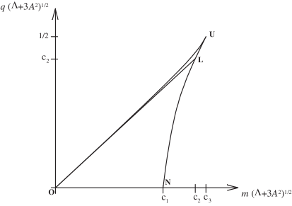
Figure 1: Relation $q\sqrt{\Lambda+3A^{2}}$ vs $m\sqrt{\Lambda+3A^{2}}$ for a fixed value of $A$ and $\Lambda$ for the four dS C instantons. $OL$ represents the lukewarm C instanton ($m=q$), $OU$ represents the cold C instanton, $NLU$ represents the Nariai C instanton, and $U$ represents the ultracold C instanton. Point $N$ represents the neutral Nariai C instanton, the only instanton for the uncharged case. When we set $\Lambda=0$ we obtain the charge/mass relation of the flat C-metric and flat Ernst instantons, and setting $A=0$ yields the charge/mass relation for the dS instantons MannRoss . This reveals the close link that exists between the instantons that describe the pair creation process in different backgrounds. $c_{1}=1/3$, $c_{2}=\sqrt{3}/4$ and $c_{3}=\sqrt{2}/3$.

IV Calculation of the black hole pair creation rates

In the last section we have found the regular dS C instantons that can be interpreted as describing a circular motion in the Euclidean sector of the solution with a period $\beta$. Each of these instantons is the Euclidean continuation of a Lorentzian solution that describes a pair of black holes that start at rest at the creation moment, and then run hyperbolically in opposite directions, due to a string that accelerates them. Now, in order to compute the pair creation rate of the corresponding black holes, we have to slice the instanton, the Euclidean trajectory, in half along $\tau=0$ and $\tau=\beta/2$, where the velocities vanish. The resulting geometry is precisely that of the moment of closest approach of the black holes in the Lorentzian sector of the dS C-metric, and in this way the Euclidean and Lorentzian solutions smoothly match together. In particular, the extrinsic curvature vanishes for both surfaces and therefore, they can be glued to each other.

In this section, we will compute the black hole pair creation rates given in (4) or (5) for each one of the four cases considered in Sec. III. Moreover, we will also compute the pair creation rate of black holes whose nucleation process is described by sub-maximal instantons. For the reason explained in Sec. II, the magnetic action will be evaluated using (6), while the electric action will be computed using (7). In general, in (6) and (7) we identify $\Sigma=\partial{\cal{M}}$ with the surfaces of zero extrinsic curvature discussed just above. It then follows that the boundary term $\int_{\Sigma}d^{3}x\sqrt{h}\,K$ vanishes. However, as we already mentioned in Sec. s III.2 and III.4, in the cold and ultracold case we have in addition an internal infinity boundary, $\Sigma^{\rm int}_{\infty}$, for which the boundary action term does not necessarily vanish.

The domain of validity of our results is the particle limit, $mA\ll 1$, for which the radius of the black hole, $r_{+}\sim m$, is much smaller than the typical distance between the black holes at the creation moment, $\ell\sim 1/A$.

In order to compute the black hole pair creation rate given by (4) or (5), we need to find $I_{\rm string}$ and $I_{\rm dS}$. The evaluation of the action of the string instanton that mediates the nucleation of a string in the dS spacetime is done using (14) and (15), yielding

$$I_{\rm string} = -\frac{1}{16\pi}\int_{\cal{M}}d^{4}x\sqrt{g}\left(R-2\Lambda\right)$$ (50)

$$= -\frac{3\pi}{2\Lambda}\frac{{\cal G}^{\prime}(x_{\rm s})}{|{\cal G}^{\prime}(x_{\rm n})|}\,,$$

where the integration over $\tau$ has been done in the interval $[0,\beta_{\rm 0}/2]$ with $\beta_{\rm 0}=2\pi/\sqrt{1+\Lambda/(3A_{0}^{\,2})}$, the integration range of $x$ was $[-1,1]$, the integration interval of $y$ was $[\sqrt{1+\Lambda/(3A_{0}^{\,2})}\,,\infty]$, and $R=4\Lambda$.

The action of the $S^{4}$ gravitational instanton that mediates the nucleation of the dS spacetime is BoussoHawk ; VolkovWipf

$$I_{\rm dS}=-\frac{3\pi}{2\Lambda}\,.$$ (51)

The nucleation rate of a string in a dS background is then given by (3). For the particle limit, $mA\ll 1$, the mass density of the string, $\mu$, is given by $\mu\simeq mA$ and

$$\Gamma_{\rm string/dS}\sim e^{-12\pi\frac{\mu}{\Lambda}}\>.$$ (52)

Thus, the nucleation probability of a string in the dS background decreases when its mass density increases.

IV.1 The lukewarm C pair creation rate

We first consider the magnetic case, whose Euclidean action is given by (6), and then we consider the electric case, using (7), and we verify that these two quantities give the same numerical value. The boundary $\Sigma=\partial\cal{M}$ that appears in (6) consists of an initial spatial surface at $\tau=0$ plus a final spatial surface at $\tau=\beta_{\rm\ell}/2$. We label these two 3-surfaces by $\Sigma_{\tau}$. Each one of these two spatial 3-surfaces is delimitated by a 2-surface at the acceleration horizon and by a 2-surface at the outer black hole horizon. The two surfaces $\Sigma_{\tau}$ are connected by a timelike 3-surface that intersects $\Sigma_{\tau}$ at the frontier $y_{A}$ and by a timelike 3-surface that intersects $\Sigma_{\tau}$ at the frontier $y_{+}$. We label these two timelike 3-surfaces by $\Sigma_{h}$. Thus $\Sigma=\Sigma_{\tau}+\Sigma_{h}$, and the region $\cal{M}$ within it is compact. With the analysis of section III.1, we can compute all the terms of action (6). We start with

$$\!\!\!\!\!\!\!\!\!\!\!\!\!\!-\frac{1}{16\pi}\int_{\cal{M}}d^{4}x\sqrt{g}\left(R-2\Lambda\right)=$$

$$\!\!\!\!\!\!\!-\frac{1}{16\pi}\int_{\Delta\phi_{\rm\ell}}\!\!\!\!d\phi\int_{0}^{\beta_{\rm\ell}/2}\!\!\!\!d\tau\int_{x_{\mathrm{s}}}^{x_{\mathrm{n}}}\!\!\!\!dx\int_{y_{A}}^{y_{+}}\!\!\!\!dy\frac{2\Lambda}{\left[A(x+y)\right]^{4}}\>,$$ (53)

where we have used $R=4\Lambda$, and $y_{A}$ and $y_{+}$ are given by (19), $x_{\mathrm{s}}$ and $x_{\mathrm{n}}$ are defined by (III.1), and $\beta_{\rm\ell}$ and $\Delta\phi_{\rm\ell}$ are respectively given by (22) and (25). The Maxwell term in the action yields

$$\!\!\!\!\!\!\!\!\!\frac{1}{16\pi}\int_{\cal{M}}\!\!d^{4}x\sqrt{g}\>F_{\rm mag}^{2}\!=\!\frac{q^{2}}{16\pi}\,\Delta\phi_{\rm\ell}\,\beta_{\rm\ell}\,(x_{\mathrm{n}}-x_{\mathrm{s}})(y_{+}-y_{A})\>,$$

(54)

where we have used $F_{\rm mag}^{2}=2q^{2}A^{4}(x+y)^{4}$ [see (10)], and $\int_{\Sigma}d^{3}x\sqrt{h}\,K=0$. Adding all these terms yields for the magnetic action (6)

$$\!\!\!\!\!\!\!\!\!\!I_{\rm mag}^{\rm\ell} = -\frac{3\pi}{16\Lambda}\frac{1}{8mA}\left(1-\sqrt{\frac{1-4mA}{1+4mA}}\right)$$ (55)

$$\!\!\!\!\!\times\left(1+\sqrt{1-(4mA)^{2}}-\frac{4m}{\sqrt{3}}\sqrt{\Lambda+3A^{2}}\right)\,,$$

and, given that the string is already present in the initial system, the pair creation rate of nonextreme lukewarm black holes when the cosmic string breaks is

$$\Gamma_{\rm BHs/string}^{\rm\ell}=\eta\,e^{-2I_{\rm mag}^{\rm\ell}+2I_{\rm string}}\,,$$ (56)

where (50) yields $I_{\rm string}=-\frac{3\pi}{2\Lambda}\frac{\sqrt{1-4mA}}{\sqrt{1+4mA}}$, and $\eta$ is the one-loop contribution not computed here. $I_{\rm mag}^{\rm\ell}$ is a monotonically increasing function of both $m$ and $A$ (for a fixed $\Lambda$). When we take the limit $A=0$ of (55) we get

$$I_{\rm mag}^{\rm\ell}{\biggl{|}}_{A\rightarrow 0}=-\frac{3\pi}{2\Lambda}+\pi\,m\sqrt{\frac{3}{\Lambda}}\,,$$ (57)

recovering the action for the $A=0$ lukewarm instanton MannRoss , that describes the pair creation of two non-extreme dS$-$Reissner-Nordström black holes accelerated only by the cosmological constant.

In the electric case, the Euclidean action is given by (7) with $F_{\rm el}^{2}=-2q^{2}A^{4}(x+y)^{4}$ [see (11)]. Thus,

$$\frac{1}{16\pi}\int_{\cal{M}}d^{4}x\sqrt{g}\>F_{\rm el}^{2}=-\frac{1}{16\pi}\int_{\cal{M}}d^{4}x\sqrt{g}\>F_{\rm mag}^{2}\>.$$ (58)

In order to compute the extra Maxwell boundary term in (7) we have to find a vector potential, $A_{\nu}$, that is regular everywhere including at the horizons. An appropriate choice in the lukewarm case is $A_{y}=-i\,q\,\tau$, which obviously satisfies (11). The integral over $\Sigma$ consists of an integration between $y_{A}$ and $y_{+}$ along the $\tau=0$ surface and back along $\tau=\beta_{\rm\ell}/2$, and of an integration between $\tau=0$ and $\tau=\beta_{\rm\ell}/2$ along the $y=y_{+}$ surface and back along the $y=y_{A}$ surface. The normal to $\Sigma_{\tau}$ is $n_{\mu}=(\sqrt{{\cal{F}}}/[A(x+y)],0,0,0)$, and the normal to $\Sigma_{h}$ is $n_{\mu}=(0,\sqrt{{\cal{F}}}/[A(x+y)],0,0)$. Thus $F^{\mu\nu}n_{\mu}A_{\nu}=0$ on $\Sigma_{h}$, and the non-vanishing contribution comes only from the integration along the $\tau=\beta_{\rm\ell}/2$ surface. The Maxwell boundary term in (7), $-\frac{1}{4\pi}\int_{\Sigma}d^{3}x\sqrt{h}\,F^{\mu\nu}n_{\mu}A_{\nu}$, is then

$$\!\!\!\!\!\!\!\!\!\!\!\!\!\!\!\!\!\!\!\!\!\!\!\!\!\!\!\!\!-\frac{1}{4\pi}\int_{\Sigma_{\tau=\beta_{\rm\ell}/2}}\!\!\!\!d^{3}x\sqrt{g_{yy}g_{xx}g_{\phi\phi}}\>F^{\tau y}n_{\tau}A_{y}=$$

$$\>\>\>\>\>\>\>\>\>\>\frac{q^{2}}{8\pi}\,\Delta\phi_{\rm\ell}\,\beta_{\rm\ell}\,(x_{\mathrm{n}}-x_{\mathrm{s}})(y_{+}-y_{A})\>.$$ (59)

Adding (53), (58) and (59) yields for the electric action (7)

$$I_{\rm el}^{\rm\ell}=I_{\rm mag}^{\rm\ell}\,,$$ (60)

where $I_{\rm mag}^{\rm\ell}$ is given by (55).

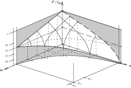
Figure 2: Plot of $I^{\rm\ell}/I_{\rm dS}$ as a function of $m$ and $A$ for a fixed $\Lambda$, where $I^{\rm\ell}$ is the action of the lukewarm C instanton, given in (55), and $I_{\rm dS}=-\frac{3\pi}{2\Lambda}$ is the action of de Sitter space. See text of Sec. IV.1. $m_{1}=1/(3\sqrt{\Lambda})$, $m_{2}=\sqrt{3}/(4\sqrt{\Lambda})$ and $m_{3}=\sqrt{2}/(3\sqrt{\Lambda})$.

In Fig. 2 we show a plot of $I^{\rm\ell}/I_{\rm dS}$ as a function of $m$ and $A$ for a fixed $\Lambda$, where $I_{\rm dS}=-\frac{3\pi}{2\Lambda}$ is the action of de Sitter space. Given the pair creation rate, $\Gamma_{\rm BHs/string}^{\rm\ell}\propto e^{-2I_{\rm mag}^{\rm\ell}+2I_{\rm string}}$, we conclude that, for a fixed $\Lambda$ and $A$, as the mass and charge of the lukewarm black holes increase, the probability they have to be pair created decreases monotonically. Moreover, for a fixed mass and charge, this probability increases monotonically as the acceleration provided by the string increases. Alternatively, we can discuss the behavior of $\Gamma_{\rm BHs/dS}^{\rm\ell}\propto e^{-2I_{\rm mag}^{\rm\ell}+2I_{\rm dS}}$. In this case, for a fixed mass and charge, the probability decreases monotonically as the acceleration of the black holes increases.

IV.2 The cold C pair creation rate

We first consider the magnetic case, whose Euclidean action is given by (6). The boundary that appears in (6) is given by $\Sigma=\Sigma_{\tau}+\Sigma_{h}+\Sigma^{\rm int}_{\infty}$, where $\Sigma_{\tau}$ is a spatial surface at $\tau=0$ and $\tau=\beta_{\rm c}/2$, $\Sigma_{h}$ is a timelike 3-surface at $y=y_{A}$, and the timelike 3-surface $\Sigma^{\rm int}_{\infty}$ is an internal infinity boundary at $y=y_{+}=\rho$. With the analysis of Sec. III.2, we can compute all the terms of action (6). We start with

$$\!\!\!\!\!\!\!\!\!\!\!\!\!\!-\frac{1}{16\pi}\int_{\cal{M}}d^{4}x\sqrt{g}\left(R-2\Lambda\right)=$$

$$\!\!\!\!\!\!\!-\frac{1}{16\pi}\int_{\Delta\phi_{\rm c}}\!\!\!\!d\phi\int_{0}^{\beta_{\rm c}/2}\!\!\!\!d\tau\int_{x_{\mathrm{s}}}^{x_{\mathrm{n}}}\!\!\!\!dx\int_{y_{A}}^{\rho}\!\!\!\!dy\frac{2\Lambda}{\left[A(x+y)\right]^{4}}\>,$$ (61)

where we have used $R=4\Lambda$, and $\rho$ and $y_{A}$ are respectively given by (28) and (30), $x_{\mathrm{s}}$ and $x_{\mathrm{n}}$ are defined by (36), and $\beta_{\rm c}$ and $\Delta\phi_{\rm c}$ are, respectively, given by (35) and (12). The Maxwell term in the action yields

$$\!\!\!\!\!\!\!\!\!\!\!\frac{1}{16\pi}\int_{\cal{M}}\!\!d^{4}x\sqrt{g}\>F_{\rm mag}^{2}\!=\!\frac{q^{2}}{16\pi}\,\Delta\phi_{\rm c}\,\beta_{\rm c}\,(x_{\mathrm{n}}-x_{\mathrm{s}})(\rho-y_{A})\>,$$

(62)

where we have used $F_{\rm mag}^{2}=2q^{2}A^{4}(x+y)^{4}$ [see (10)], and $\int_{\Sigma}d^{3}x\sqrt{h}\,K=0$. Adding all these terms yields for the magnetic action (6) of the cold case

$$I_{\rm mag}^{\rm c}=-\frac{\Delta\phi_{\rm c}}{8A^{2}}\,\frac{x_{\mathrm{n}}-x_{\mathrm{s}}}{(x_{\mathrm{n}}+y_{A})(x_{\mathrm{s}}+y_{A})}\,.$$ (63)

Given that the string is already present in the initial system, the pair creation rate of extreme cold black holes when the string breaks is $\Gamma_{\rm BHs/string}^{\rm c}=\eta\,e^{-2I_{\rm mag}^{\rm c}+2I_{\rm string}}$, where $I_{\rm string}$ is given by (50), and $\eta$ is the one-loop contribution not computed here. In Fig. 3 we show a plot of $I_{\rm mag}^{\rm c}/I_{\rm dS}$ as a function of $m$ and $A$ for a fixed $\Lambda$. Given the pair creation rate, $\Gamma_{\rm BHs/string}^{\rm c}$, we conclude that for a fixed $\Lambda$ and $A$ as the mass and charge of the cold black holes increases, the probability they have to be pair created decreases monotonically. Moreover, for a fixed mass and charge, this probability increases monotonically as the acceleration of the black holes increases. Alternatively, we can discuss the behavior of $\Gamma_{\rm BHs/dS}^{\rm c}\propto e^{-2I_{\rm mag}^{\rm c}+2I_{\rm dS}}$. In this case, for a fixed mass and charge, the probability decreases monotonically as the acceleration of the black holes increases. When we take the limit $A=0$ we recover the action for the $A=0$ cold instanton MannRoss , which lies in the range $-\frac{3\pi}{2\Lambda}\leq I_{\rm mag}^{\rm c}{\bigl{|}}_{A\rightarrow 0}\leq-\frac{\pi}{4\Lambda}$, and which describes the pair creation of extreme dS$-$Reissner-Nordström black holes accelerated only by the cosmological constant.

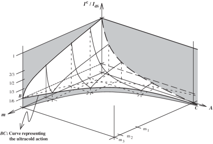
Figure 3: Plot of $I^{\rm c}/I_{\rm dS}$ as a function of $m$ and $A$ for a fixed $\Lambda$, where $I^{\rm c}$ is the action of the cold C instanton, given in (63), and $I_{\rm dS}=-\frac{3\pi}{2\Lambda}$ is the action of de Sitter space (see text of Sec. IV.2). The plot for the ultracold C action, given in (74), is also represented by the curve $BC$ (see text of Sec. IV.4). $m_{1}=1/(3\sqrt{\Lambda})$, $m_{2}=\sqrt{3}/(4\sqrt{\Lambda})$ and $m_{3}=\sqrt{2}/(3\sqrt{\Lambda})$.

In the electric case, the Euclidean action is given by (7) with $F_{\rm el}^{2}=-2q^{2}A^{4}(x+y)^{4}$ [see (11)]. Thus,

$$\frac{1}{16\pi}\int_{\cal{M}}d^{4}x\sqrt{g}\>F_{\rm el}^{2}=-\frac{1}{16\pi}\int_{\cal{M}}d^{4}x\sqrt{g}\>F_{\rm mag}^{2}\>.$$ (64)

In order to compute the extra Maxwell boundary term in (7) we have to find a vector potential, $A_{\nu}$, that is regular everywhere including at the horizons. An appropriate choice in the cold case is $A_{y}=-i\,q\,\tau$, which obviously satisfies (11). Analogously to the lukewarm case, the non-vanishing contribution to the Maxwell boundary term in (7) comes only from the integration along the $\tau=\beta_{\rm c}/2$ surface, and is given by

$$\!\!\!\!\!\!\!\!\!\!\!\!\!\!\!\!\!\!\!\!\!\!\!\!\!\!\!\!\!-\frac{1}{4\pi}\int_{\Sigma_{\tau=\beta_{\rm c}/2}}\!\!\!\!d^{3}x\sqrt{g_{yy}g_{xx}g_{\phi\phi}}\>F^{\tau y}n_{\tau}A_{y}=$$

$$\>\>\>\>\>\>\>\>\>\>\frac{q^{2}}{8\pi}\,\Delta\phi_{\rm c}\,\beta_{\rm c}\,(x_{\mathrm{n}}-x_{\mathrm{s}})(\rho-y_{A})\>.$$ (65)

Adding (64) and (65) yields (62). Thus, the electric action (7) of the cold instanton is equal to the magnetic action, $I_{\rm el}^{\rm c}=I_{\rm mag}^{\rm c}$, and therefore electric and magnetic cold black holes have the same probability of being pair created.

IV.3 The Nariai C pair creation rate

The Nariai C instanton is the only one that can have zero charge. We will first consider the charged Nariai C instanton and then the neutral Nariai C instanton.

We start with the magnetic case, whose Euclidean action is given by (6). The boundary that appears in (6) is given by $\Sigma=\Sigma_{\tilde{\tau}}+\Sigma_{h}$, where $\Sigma_{\tilde{\tau}}$ is a spatial surface at $\tilde{\tau}=0$ and $\tilde{\tau}=\pi$, and $\Sigma_{h}$ is a timelike 3-surface at $\chi=0$ and $\chi=\pi$. With the analysis of Sec. III.3, we can compute all the terms of action (6). We start with

$$\!\!\!\!\!\!\!\!\!\!\!\!\!\!-\frac{1}{16\pi}\int_{\cal{M}}d^{4}x\sqrt{g}\left(R-2\Lambda\right)=$$

$$\!\!\!\!\!\!\!\!\!\!-\frac{1}{16\pi}\int_{\Delta\phi_{\rm N}}\!\!\!\!d\phi\int_{0}^{\pi}\!\!\!\!d\tilde{\tau}\int_{x_{\mathrm{s}}}^{x_{\mathrm{n}}}\!\!\!\!dx\int_{0}^{\pi}\!\!\!\!d\chi\>\frac{2\Lambda\sin\chi}{\left[A(x+\rho)\right]^{4}{\cal{K}}}\>,$$ (66)

where we have used $R=4\Lambda$, $x_{\mathrm{s}}$ and $x_{\mathrm{n}}$ are defined by (36), and $\Delta\phi_{\rm N}$ is given by (12). The Maxwell term in the action yields

$$\frac{1}{16\pi}\int_{\cal{M}}d^{4}x\sqrt{g}\>F_{\rm mag}^{2}=\frac{q^{2}}{4\,\cal{K}}\,\Delta\phi_{\rm N}\,(x_{\mathrm{n}}-x_{\mathrm{s}})\>,$$ (67)

where we have used $F_{\rm mag}^{2}=2q^{2}A^{4}(x+\rho)^{4}$ [see (10)], and $\int_{\Sigma}d^{3}x\sqrt{h}\,K=0$. Adding these three terms yields the magnetic action (6) of the Nariai case

$$I_{\rm mag}^{\rm N}=-\,\frac{\Delta\phi_{\rm N}}{4A^{2}}\,\frac{x_{\mathrm{n}}-x_{\mathrm{s}}}{(x_{\mathrm{n}}+\rho)(x_{\mathrm{s}}+\rho)}\,,$$ (68)

where $m$ and $q$ are subjected to (40). Given that the string is already present in the initial system, the pair creation rate of extreme Nariai black holes when the string breaks is $\Gamma_{\rm BHs/string}^{\rm N}=\eta\,e^{-2I_{\rm mag}^{\rm N}+2I_{\rm string}}$, where $I_{\rm string}$ is given by (50), and $\eta$ is the one-loop contribution not computed here. In Fig. 4 we show a plot of $I_{\rm mag}^{\rm N}/I_{\rm dS}$ as a function of $m$ and $A$ for a fixed $\Lambda$. Given the pair creation rate, $\Gamma_{\rm BHs/string}^{\rm N}$, we conclude that for a fixed $\Lambda$ and $A$ as the mass and charge of the Nariai black holes increases, the probability they have to be pair created decreases monotonically. Moreover, for a fixed mass and charge, this probability increases monotonically as the acceleration of the black holes increases. Alternatively, we can discuss the behavior of $\Gamma_{\rm BHs/dS}^{\rm N}\propto e^{-2I_{\rm mag}^{\rm N}+2I_{\rm dS}}$. In this case, for a fixed mass and charge, the probability decreases monotonically as the acceleration of the black holes increases. When we take the limit $A=0$ we recover the action for the $A=0$ Nariai instanton MannRoss ; HawkRoss , which lies in the range $-\frac{\pi}{\Lambda}\leq I_{\rm mag}^{\rm N}{\bigl{|}}_{A\rightarrow 0}\leq-\frac{\pi}{2\Lambda}$, and that describes the nucleation of a Nariai universe that is unstable GinsPerry ; BoussoHawk ; Bousso60y and decays through the pair creation of extreme dS$-$Reissner-Nordström black holes accelerated only by the cosmological constant.

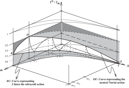
Figure 4: Plot of $I^{\rm N}/I_{\rm dS}$ as a function of $m$ and $A$ for a fixed $\Lambda$, where $I^{\rm N}$ is the action of the cold C instanton, given in (68), and $I_{\rm dS}=-\frac{3\pi}{2\Lambda}$ is the action of de Sitter space. The neutral Nariai plot is sketched by the curve $DE$ (see text of Sec. IV.3). The curve $BC$ represents two times the ultracold C action, given in (74). $m_{1}=1/(3\sqrt{\Lambda})$, $m_{2}=\sqrt{3}/(4\sqrt{\Lambda})$ and $m_{3}=\sqrt{2}/(3\sqrt{\Lambda})$.

In the electric case, the Euclidean action is given by (7) with $F_{\rm el}^{2}=-2q^{2}A^{4}(x+\rho)^{4}$ [see (44)]. Thus,

$$\frac{1}{16\pi}\int_{\cal{M}}d^{4}x\sqrt{g}\>F_{\rm el}^{2}=-\frac{1}{16\pi}\int_{\cal{M}}d^{4}x\sqrt{g}\>F_{\rm mag}^{2}\>.$$ (69)

In order to compute the extra Maxwell boundary term in (7), the appropriate vector potential, $A_{\nu}$, that is regular everywhere including at the horizons is $A_{\chi}=i\,\frac{q}{\cal{K}}\,\tilde{\tau}\,\sin\chi$, which obviously satisfies (44). The integral over $\Sigma$ consists of an integration between $\chi=0$ and $\chi=\pi$ along the $\tilde{\tau}=0$ surface and back along $\tilde{\tau}=\pi$, and of an integration between $\tilde{\tau}=0$ and $\tilde{\tau}=\pi$ along the $\chi=0$ surface, and back along the $\chi=\pi$ surface. The unit normal to $\Sigma_{\tilde{\tau}}$ is $n_{\mu}=(\frac{\sin\chi}{\sqrt{\cal{K}}A(x+\rho)},0,0,0)$, and $F^{\mu\nu}n_{\mu}A_{\nu}=0$ on $\Sigma_{h}$. Therefore, the non-vanishing contribution to the Maxwell boundary term in (7), $-\frac{1}{4\pi}\int_{\Sigma}d^{3}x\sqrt{h}\,F^{\mu\nu}n_{\mu}A_{\nu}$, comes only from the integration along the $\tilde{\tau}=\pi$ surface and is given by

$$-\frac{1}{4\pi}\int_{\Sigma_{\tilde{\tau}=\pi}}\!\!\!\!\!\!d^{3}x\sqrt{h}\>F^{\tilde{\tau}\chi}n_{\tilde{\tau}}A_{\chi}=\frac{q^{2}}{2\,\cal{K}}\,\Delta\phi_{\rm N}\,(x_{\mathrm{n}}-x_{\mathrm{s}})\>.$$ (70)

Adding (69) and (70) yields (67). So, the electric action (7) of the charged Nariai instanton is equal to the magnetic action, $I_{\rm el}^{\rm N}=I_{\rm mag}^{\rm N}$, and therefore electric and magnetic charged Nariai black holes have the same probability of being pair created.

Now, we discuss the neutral Nariai C instanton. This instanton is particulary important since it is the only regular Euclidean solution available when we want to evaluate the pair creation of neutral black holes. The same feature is present in the $A=0$ case where only the neutral Nariai instanton is available GinsPerry ; MannRoss ; BoussoHawk ; VolkovWipf . The action of the neutral Nariai C instanton is simply given by (66) and, for a fixed $\Lambda$ and $A$, it is always smaller than the action of the charged Nariai C instanton (see line $DE$ in Fig. 4): $I_{\rm charged}^{\rm N}>I_{\rm neutral}^{\rm N}>I_{\rm dS}$. Thus the pair creation of charged Nariai black holes is suppressed relative to the pair creation of neutral Nariai black holes, and both are suppressed relative to the dS space.

IV.4 The ultracold C pair creation rate

We first consider the magnetic case, whose Euclidean action is given by (6). The boundary that appears in (6) is given by $\Sigma=\Sigma_{\tilde{\tau}}+\Sigma_{h}+\Sigma^{\rm int}_{\infty}$, where $\Sigma_{\tilde{\tau}}$ is a spatial surface at $\tilde{\tau}=0$ and $\tilde{\tau}=\pi$, $\Sigma_{h}$ is a timelike 3-surface at the Rindler horizon $\chi=0$, and the timelike 3-surface $\Sigma^{\rm int}_{\infty}$ is an internal infinity boundary at $\chi=\infty$. With the analysis of Sec. III.4, we can compute all the terms of action (6). We start with $-\frac{1}{16\pi}\int_{\cal{M}}d^{4}x\sqrt{g}\left(R-2\Lambda\right)$ which yields (using $R=4\Lambda$)

$$\!\!\!\!\!\!\!\!\!\!\!\!\!\!\!\!\!\!\!\!\!\!\!\!\!-\frac{1}{16\pi}\int_{\Delta\phi_{\rm u}}\!\!\!\!d\phi\int_{0}^{\pi}\!\!\!\!d\tilde{\tau}\int_{x_{\mathrm{s}}}^{x_{\mathrm{n}}}\!\!\!\!dx\int_{0}^{\chi_{0}}\!\!\!\!d\chi\>\frac{2\Lambda\chi}{(Ax+\rho)^{4}}=$$

$$-\frac{\Lambda}{16}\>\Delta\phi_{\rm u}\>\chi_{0}^{2}\>\int_{x_{\mathrm{s}}}^{x_{\mathrm{n}}}\!\!\!\!dx\frac{1}{(Ax+A\rho)^{4}}{\biggl{|}}_{\chi_{0}\rightarrow\infty}\>,$$ (71)

where $x_{\mathrm{s}}$ and $x_{\mathrm{n}}$ are defined by (36) and (47), and $\Delta\phi_{\rm u}$ is given by (12). The Maxwell term in the action yields

$$\frac{1}{16\pi}\int_{\cal{M}}d^{4}x\sqrt{g}\>F_{\rm mag}^{2}=\frac{q^{2}}{16}\,\Delta\phi_{\rm u}\>\chi_{0}^{2}\,(x_{\mathrm{n}}-x_{\mathrm{s}}){\biggl{|}}_{\chi_{0}\rightarrow\infty}\!\!\!\!,$$ (72)

where we have used $F_{\rm mag}^{2}=2q^{2}A^{4}(x+\rho)^{4}$ [see (10)] with $\rho=\sqrt{2(\Lambda+3A^{2})}$. Due to the fact that $\chi_{0}\rightarrow\infty$ it might seem that the contribution from (71) and (72) diverges. Fortunately this is not the case since these two terms cancel each other. Trying to verify this analytically is cumbersome, but for our purposes we can simply fix any numerical value for $\Lambda$ and $A$, and using (47) and (36) we indeed verify that (71) and (72) cancel each other.

Now, contrary to the other instantons, the ultracold C instanton has a non-vanishing extrinsic curvature boundary term, $-\frac{1}{16\pi}\int_{\Sigma}d^{3}x\sqrt{h}\,K\neq 0$, due to the internal infinity boundary ($\Sigma^{\rm int}_{\infty}$ at $\chi=\infty$) contribution. The extrinsic curvature to $\Sigma^{\rm int}_{\infty}$ is $K_{\mu\nu}=h_{\mu}^{\>\>\>\alpha}\nabla_{\alpha}n_{\nu}$, where $n_{\nu}=(0,\frac{1}{A(x+\rho)},0,0)$ is the unit outward normal to $\Sigma^{\rm int}_{\infty}$, $h_{\mu}^{\>\>\>\alpha}=g_{\mu}^{\>\>\>\alpha}-n_{\mu}n^{\alpha}=(1,0,1,1)$ is the projection tensor onto $\Sigma^{\rm int}_{\infty}$, and $\nabla_{\alpha}$ represents the covariant derivative with respect to $g_{\mu\nu}$. Thus the trace of the extrinsic curvature to $\Sigma^{\rm int}_{\infty}$ is $K=g^{\mu\nu}K_{\mu\nu}=A(x+\rho)/\chi$, and

$$\!\!\!\!\!\!\!\!\!\!\!\!\!\!-\frac{1}{8\pi}\int_{\Sigma}d^{3}x\sqrt{h}\,K=$$

$$-\frac{1}{8\pi}\,\int_{\Delta\phi_{\rm u}}\!\!\!\!d\phi\int_{0}^{\pi}\!\!\!\!d\tilde{\tau}\int_{x_{\mathrm{s}}}^{x_{\mathrm{n}}}\!\!\!\!dx\>\frac{1}{(Ax+A\rho)^{2}}.$$ (73)

The magnetic action (6) of the ultracold C instanton is then

$$\!\!\!\!\!\!\!\!I_{\rm mag}^{\rm u}=$$

$$\!\!\!\!\!-\frac{\pi}{4}\left[x_{\mathrm{n}}\left(1+A\sqrt{\frac{2}{\Lambda+3A^{2}}}\,x_{\mathrm{n}}+\frac{A^{2}}{2(\Lambda+3A^{2})}x_{\mathrm{n}}^{2}\right)\right]^{-1}$$

$$\!\!\!\!\!\times\frac{x_{\mathrm{n}}-x_{\mathrm{s}}}{\left[Ax_{\mathrm{n}}+\sqrt{2(\Lambda+3A^{2})}\right]\left[Ax_{\mathrm{s}}+\sqrt{2(\Lambda+3A^{2})}\right]}\,,$$ (74)

where $x_{\mathrm{s}}$ and $x_{\mathrm{n}}$ are defined by (36) and (47). When we take the limit $A=0$ we get $x_{\mathrm{s}}=-1$ and $x_{\mathrm{n}}=1$, and

$$I_{\rm mag}^{\rm u}{\biggl{|}}_{A\rightarrow 0}=-\frac{\pi}{4\Lambda}\,,$$ (75)

and therefore we recover the action for the $A=0$ ultracold instanton MannRoss , that describes the pair creation of ultracold black holes accelerated only by the cosmological constant.

In Fig. 2 we show a plot of $I_{\rm mag}^{\rm u}/I_{\rm dS}$ as a function of $m$ and $A$ for a fixed $\Lambda$. When we fix $\Lambda$ and $A$ we also fix the mass and charge of the ultracold black holes. For a fixed $\Lambda$, when $A$ increases the probability of pair creation of ultracold black holes, $\Gamma_{\rm BHs/string}^{\rm u}$, increases monotonically and they have a lower mass and charge. Alternatively, we can discuss the behavior of $\Gamma_{\rm BHs/dS}^{\rm u}$. In this case, the probability decreases monotonically as the acceleration of the black holes increases.

In the electric case, the Euclidean action is given by (7) with $F_{\rm el}^{2}=-2q^{2}A^{4}(x+\rho)^{4}$ [see (49)]. Thus,

$$\frac{1}{16\pi}\int_{\cal{M}}d^{4}x\sqrt{g}\>F_{\rm el}^{2}=-\frac{1}{16\pi}\int_{\cal{M}}d^{4}x\sqrt{g}\>F_{\rm mag}^{2}\>.$$ (76)

In the ultracold case the vector potential $A_{\nu}$, that is regular everywhere including at the horizon, needed to compute the extra Maxwell boundary term in (7) is $A_{\tilde{\tau}}=i\,\frac{q}{2}\,\chi^{2}$, which obviously satisfies (49). The integral over $\Sigma$ consists of an integration between $\chi=0$ and $\chi=\infty$ along the $\tilde{\tau}=0$ surface and back along $\tilde{\tau}=\pi$, and of an integration between $\tilde{\tau}=0$ and $\tilde{\tau}=\pi$ along the $\chi=0$ surface, and back along the internal infinity surface $\chi=\infty$. The non-vanishing contribution to the Maxwell boundary term in (7) comes only from the integration along the internal infinity boundary $\Sigma^{\rm int}_{\infty}$, and is given by

$$\!\!\!\!\!\!\!\!\!\!\!\!\!\!\!\!\!\!\!\!\!\!\!\!\!\!\!\!\!-\frac{1}{4\pi}\int_{\Sigma^{\rm int}_{\infty}}d^{3}x\sqrt{g_{\tilde{\tau}\tilde{\tau}}g_{xx}g_{\phi\phi}}\>F^{\chi\tilde{\tau}}n_{\chi}A_{\tilde{\tau}}=$$

$$\>\>\>\>\>\>\>\>\>\>\>\>\>\>\>\>\>\>\>\>\frac{q^{2}}{8}\,\Delta\phi_{\rm u}\>\chi_{0}^{2}\,(x_{\mathrm{n}}-x_{\mathrm{s}}){\biggl{|}}_{\chi_{0}\rightarrow\infty}\>.$$ (77)

Adding (76) and (77) yields (72). Thus, the electric action (7) of the ultracold C instanton is equal to the magnetic action, $I_{\rm el}^{\rm u}=I_{\rm mag}^{\rm u}$, and therefore electric and magnetic ultracold black holes have the same probability of being pair created.

IV.5 Pair creation rate of nonextreme sub-maximal black holes

The lukewarm, cold, Nariai and ultracold C-metric instantons are saddle point solutions free of conical singularities both in the $y_{+}$ and $y_{A}$ horizons. The corresponding black holes may then nucleate in the dS background when a cosmic string breaks, and we have computed their pair creation rates in the last four subsections. However, these particular black holes are not the only ones that can be pair created. Indeed, it has been shown in WuSubMax ; BoussoHawkSubMax that Euclidean solutions with conical singularities may also be used as saddle points for the pair creation process. In this way, pair creation of nonextreme sub-maximal black holes is allowed (by this nomenclature we mean all the nonextreme black holes other than the lukewarm ones that are in the region interior to the close line $NOUN$ in Fig. 1), and their pair creation rate may be computed. In order to calculate this rate, the action is given by (6) and (7) (in the magnetic and electric cases respectively) and, in addition, it has now an extra contribution from the conical singularity (c.s.) that is present in one of the horizons ($y_{+}$, say) given by ReggeGibbonsPerryAconSing ; GinsPerry

$$\frac{1}{16\pi}\int_{\cal{M}}d^{4}x\sqrt{g}\>\left(R-2\Lambda\right){\biggl{|}}_{{\rm c.s.}\>{\rm at}\>y_{+}}\!\!\!=\frac{{\cal A}_{+}\>\delta}{16\pi}\>,$$ (78)

where ${\cal A}_{+}=\int_{y=y_{+}}\sqrt{g_{xx}g_{\phi\phi}}\>dx\,d\phi$ is the area of the 2-surface spanned by the conical singularity, and

$$\delta=2\pi\left(1-\frac{\beta_{A}}{\beta_{+}}\right)$$ (79)

is the deficit angle associated to the conical singularity at the horizon $y_{+}$, with $\beta_{A}=4\pi/|{\cal F}^{\prime}(y_{A})|$ and $\beta_{+}=4\pi/|{\cal F}^{\prime}(y_{+})|$ being the periods of $\tau$ that avoid a conical singularity in the horizons $y_{A}$ and $y_{+}$, respectively. The contribution from (6) and (7) follows straightforwardly in a similar way as the one shown in subsection IV.1 with the period of $\tau$, $\beta_{A}$, chosen in order to avoid the conical singularity at the acceleration horizon, $y=y_{A}$. The full Euclidean action for general nonextreme sub-maximal black holes is then

$$\!\!\!\!\!\!\!\!I\!=\!\frac{\Delta\phi}{A^{2}}\,\left(\!\frac{x_{\mathrm{n}}-x_{\mathrm{s}}}{(x_{\mathrm{n}}+y_{A})(x_{\mathrm{s}}+y_{A})}\!+\!\frac{x_{\mathrm{n}}-x_{\mathrm{s}}}{(x_{\mathrm{n}}+y_{+})(x_{\mathrm{s}}+y_{+})}\!\right),$$

(80)

where $\Delta\phi$ is given by (12), and the pair creation rate of nonextreme sub-maximal black holes is given by (4) or (5) with the use of (50) and (51). In order to compute (80), we need the relation between the parameters $A$, $\Lambda$, $m$, $q$, and the horizons $y_{A}$, $y_{+}$ and $y_{-}$. In general, for a nonextreme solution with horizons $y_{A}<y_{+}<y_{-}$, one has

$${\cal F}(y)=-\frac{1}{\mu}(y-y_{A})(y-y_{+})(y-y_{-})(ay+b)\>,$$ (81)

with

$$\mu\!\! = \!\!y_{A}y_{+}y_{-}(y_{A}+y_{+}+y_{-})+(y_{A}y_{+}+y_{A}y_{-}+y_{+}y_{-})^{2}$$

$$a\!\! = \!\!\left(y_{A}y_{+}+y_{A}y_{-}+y_{+}y_{-}\right)$$

$$b\!\! = \!\!y_{A}y_{+}y_{-}\>.$$ (82)

The parameters $A$, $\Lambda$, $m$ and $q$ can be expressed as a function of $y_{A}$, $y_{+}$ and $y_{-}$ by

$$\frac{\Lambda}{3A^{2}}\!\! = \!\!\mu^{-2}(y_{A}y_{+}y_{-})^{2}-1$$

$$q^{2}A^{2}\!\! = \!\!\mu^{-1}(y_{A}y_{+}+y_{A}y_{-}+y_{+}y_{-})$$

$$mA\!\! = \!\!(2\,\sigma)^{-1}(y_{A}+y_{+})(y_{A}+y_{-})(y_{+}+y_{-})$$

$$\sigma\!\! = \!\!y_{A}^{2}y_{+}y_{-}+y_{A}y_{+}^{2}y_{-}+y_{A}y_{+}y_{-}^{2}+(y_{A}y_{+})^{2}$$ (83)

$$+(y_{A}y_{-})^{2}+(y_{+}y_{-})^{2}\>.$$

The allowed values of parameters $m$ and $q$ are those contained in the interior region defined by the close line $NOUN$ in Fig. 1.

V Entropy, area and pair creation rate

In previous works on black hole pair creation in general background fields it has been well established that the pair creation rate is proportional to the exponential of the gravitational entropy $S$ of the system, $\Gamma\propto e^{S}$, with the entropy being given by one quarter of the the total area $\cal{A}$ of all the horizons present in the instanton, $S={\cal{A}}/4$. In what follows we will verify that these relations also hold for the instantons of the dS C-metric.

V.1 The lukewarm C case. Entropy and area

In the lukewarm case, the instanton has two horizons in its Euclidean section, namely the acceleration horizon at $y=y_{A}$ and the black hole horizon at $y=y_{+}$. So, the total area of the lukewarm C instanton is

$$\cal{A}^{\rm\ell}\!\! = \!\!\int_{y=y_{A}}\!\!\!\sqrt{g_{xx}g_{\phi\phi}}\>dx\,d\phi+\int_{y=y_{+}}\!\!\!\sqrt{g_{xx}g_{\phi\phi}}\>dx\,d\phi=$$

$$\!\!\!\!\!\!\!\!\!\!\!\!\frac{\Delta\phi_{\rm\ell}}{A^{2}}\,\left(\frac{x_{\mathrm{n}}-x_{\mathrm{s}}}{(x_{\mathrm{n}}+y_{A})(x_{\mathrm{s}}+y_{A})}+\frac{x_{\mathrm{n}}-x_{\mathrm{s}}}{(x_{\mathrm{n}}+y_{+})(x_{\mathrm{s}}+y_{+})}\right)\,,$$

where $y_{A}$ and $y_{+}$ are given by (19), $x_{\mathrm{s}}$ and $x_{\mathrm{n}}$ are defined by (III.1), and $\Delta\phi_{\rm\ell}$ is given by (25). It is straightforward to verify that ${\cal{A}^{\rm\ell}}=-8I^{\rm\ell}$, where $I^{\rm\ell}$ is given by (55), and thus $\Gamma^{\rm\ell}\propto e^{S^{\rm\ell}}$, where $S^{\rm\ell}={\cal{A}^{\rm\ell}}/4$.

V.2 The cold C case. Entropy and area

In the cold case, the instanton has a single horizon, the acceleration horizon at $y=y_{A}$, in its Euclidean section, since $y=y_{+}$ is an internal infinity. So, the total area of the cold C instanton is

$$\!\!\!\!\!{\cal A}^{\rm c}\!=\int_{y=y_{A}}\!\!\!\sqrt{g_{xx}g_{\phi\phi}}\>dx\,d\phi\!=\!\frac{\Delta\phi_{\rm c}}{A^{2}}\,\frac{x_{\mathrm{n}}-x_{\mathrm{s}}}{(x_{\mathrm{n}}+y_{A})(x_{\mathrm{s}}+y_{A})}\,,$$

(85)

where $y_{A}$ is given by (30), $x_{\mathrm{s}}$ and $x_{\mathrm{n}}$ are defined by (36), and $\Delta\phi_{\rm c}$ is given by (12). Thus, ${\cal{A}^{\rm c}}=-8I^{\rm c}$, where $I^{\rm c}$ is given by (63), and thus $\Gamma^{\rm c}\propto e^{S^{\rm c}}$, where $S^{\rm c}={\cal{A}^{\rm c}}/4$.

V.3 The Nariai C case. Entropy and area

In the Nariai case, the instanton has two horizons in its Euclidean section, namely the acceleration horizon $y_{A}$ and the black hole horizon $y_{+}$, both at $y=\rho$, and thus they have the same area. So, the total area of the Nariai C instanton is

$$\!\!\!{\cal A}^{\rm N}\!\!=\!2\int_{y=\rho}\!\!\!\sqrt{g_{xx}g_{\phi\phi}}\>dx\,d\phi\!=\!2\,\frac{\Delta\phi_{\rm N}}{A^{2}}\,\frac{x_{\mathrm{n}}-x_{\mathrm{s}}}{(x_{\mathrm{n}}+\rho)(x_{\mathrm{s}}+\rho)}\,,$$

(86)

where $\sqrt{3\gamma}\leq\rho<\sqrt{6\gamma}$, $x_{\mathrm{s}}$ and $x_{\mathrm{n}}$ are defined by (36), and $\Delta\phi_{\rm N}$ is given by (12), with $m$ and $q$ subjected to (40). Thus, ${\cal{A}^{\rm N}}=-8I^{\rm N}$, where $I^{\rm N}$ is given by (68), and thus $\Gamma^{\rm N}\propto e^{S^{\rm N}}$, where $S^{\rm N}={\cal{A}^{\rm N}}/4$.

V.4 The ultracold C case. Entropy and area

In the ultracold case, the instanton has a single horizon, the Rindler horizon at $\chi=0$, in its Euclidean section, since $\chi=\infty$ is an internal infinity. So, the total area of the ultracold C instanton is

$$\!\!\!{\cal{A}}^{\rm u}\!\!=\!\!\int_{\chi=0}\!\!\!\sqrt{g_{xx}g_{\phi\phi}}\>dx\,d\phi=\!\frac{\Delta\phi_{\rm u}}{A^{2}}\,\frac{x_{\mathrm{n}}-x_{\mathrm{s}}}{(x_{\mathrm{n}}+\rho)(x_{\mathrm{s}}+\rho)}\,,$$ (87)

with $\rho=\sqrt{2(\Lambda+3A^{2})}$ [see (46)], $x_{\mathrm{s}}$ and $x_{\mathrm{n}}$ are defined by (36), and $\Delta\phi_{\rm c}$ is given by (12), with $m$ and $q$ subjected to (47). It straightforward to verify that ${\cal{A}^{\rm u}}=-8I^{\rm u}$, where $I^{\rm u}$ is given by (74), and thus $\Gamma^{\rm u}\propto e^{S^{\rm u}}$, where $S^{\rm u}={\cal{A}^{\rm u}}/4$.

As we have already said, the ultracold C instanton is a limiting case of both the charged Nariai C instanton and the cold C instanton (see, e.g., Fig. 1). Then, as expected, the action of the cold C instanton gives, in this limit, the action of the ultracold C instanton (see Fig. 3). However, the ultracold frontier of the Nariai C action is given by two times the ultracold C action (see Fig. 4). From the results of this section we clearly understand the reason for this behavior. Indeed, in the ultracold case and in the cold case, the respective instantons have a single horizon (the other possible horizon turns out to be an internal infinity). This horizon gives the only contribution to the total area, ${\cal{A}}$, and therefore to the pair creation rate. In the Nariai case, the instanton has two horizons with the same area, and thus the ultracold limit of the Nariai action is doubled with respect to the true ultracold action.

V.5 The nonextreme sub-maximal case. Entropy and area

In the lukewarm case, the instanton has two horizons in its Euclidean section, namely the acceleration horizon at $y=y_{A}$ and the black hole horizon at $y=y_{+}$. So, the total area of the saddlepoint solution is

$$\!\!\!{\cal A}=\int_{y=y_{A}}\!\!\!\sqrt{g_{xx}g_{\phi\phi}}\>dx\,d\phi+\!\int_{y=y_{+}}\!\!\!\sqrt{g_{xx}g_{\phi\phi}}\>dx\,d\phi\,,$$ (88)

and once again one has ${\cal{A}}=-8I$, where $I$ is given by (80), and thus $\Gamma\propto e^{S}$, where $S={\cal{A}}/4$.

VI Summary and discussion

We have studied in detail the quantum process in which a cosmic string breaks in a de Sitter (dS) background and a pair of black holes is created at the ends of the string. The energy to materialize and accelerate the pair comes from the positive cosmological constant and from the string tension. This process is a combination of the processes considered in MelMos -VolkovWipf , where the creation of a black hole pair in a dS background has been analyzed, and in HawkRoss-string -GregHind , where the breaking of a cosmic string accompanied by the creation of a black hole pair in a flat background has been studied. We remark that in principle our explicit values for the pair creation rates also apply to the process of pair creation in an external electromagnetic field, with the acceleration being provided in this case by the Lorentz force instead of being furnished by the string tension. Indeed, there is no dS Ernst solution, and thus we cannot discuss analytically the process. However, physically we could in principle consider an external electromagnetic field that supplies the same energy and acceleration as our strings and, from the results of the $\Lambda=0$ case (where the pair creation rates in the string and electromagnetic cases agree), we expect that the pair creation rates found in this paper do not depend on whether the energy is being provided by an external electromagnetic field or by a string.

We have constructed the saddle point solutions that mediate the pair creation process through the analytic continuation of the dS C-metric, and we have explicitly computed the nucleation rate of the process (see also a heuristic derivation of the rate in the Appendix). Globally our results state that the dS space is stable against the nucleation of a string, or against the nucleation of a string followed by its breaking and consequent creation of a black hole pair. In particular, we have answered three questions. First, we have concluded that the nucleation rate of a cosmic string in a dS background $\Gamma_{\rm string/dS}$ decreases when the mass density of the string increases. Second, given that the string is already present in our initial system, the probability $\Gamma_{\rm BHs/string}$ that it breaks and a pair of black holes is produced and accelerated apart by $\Lambda$ and by the string tension increases when the mass density of the string increases. In other words, a string with a higher mass density makes the process more probable, for a fixed black hole mass. Third, if we start with a pure dS background, the probability $\Gamma_{\rm BHs/dS}$ that a string nucleates on it and then breaks forming a pair of black holes decreases when the mass density of the string increases. These processes have a clear analogy with a thermodynamical system, with the mass density of the string being the analogue of the temperature $T$. Indeed, from the Boltzmann factor, $e^{-E_{0}/(k_{\rm B}T)}$ (where $k_{\rm B}$ is the Boltzmann constant), one knows that a higher background temperature turns the nucleation of a particle with energy $E_{0}$ more probable. However, in order to have a higher temperature we have first to furnish more energy to the background, and thus the global process (increasing the temperature to the final value $T$ plus the nucleation of the particle) becomes energetically less favorable as $T$ increases.

We have also verified that the relation between the rate, entropy and area, which is satisfied for all the black hole pair creation processes analyzed so far, also holds in the process studied in this paper. Indeed, the pair creation rate is proportional to $e^{S}$, where $S$ is the gravitational entropy of the system, and is given by one quarter of the total area of all the horizons present in the saddle point solution that mediates the pair creation.

To conclude let us recall that the dS C-metric allows two distinct physical interpretations. In one of them one removes the conical singularity at the north pole and leaves one at the south pole. In this way the dS C-metric describes a pair of black holes accelerated away by a string with positive mass density. Alternatively, we can avoid the conical singularity at the south pole and in this case the black holes are pushed away by a strut (with negative mass density) in between them, along their north poles. In this paper we have adopted the first choice. Technically, the second choice only changes the period of the angular coordinate $\phi$: it would be given by $\Delta\phi=\frac{4\pi}{|{\cal G}^{\prime}(x_{\mathrm{s}})|}$ instead of (12). We have chosen the first choice essentially for two reasons. First, the string has a positive mass density and, in this sense, it is a more physical solution than the strut. Second, in order to get the above string/pair configuration we only have to cut the string in a point. The string tension does the rest of the work. However, if we desire the strut/pair system described above we would have to cut the strut in two different points. Then we would have to discard somehow the segment that joins the black holes along their south poles.

*

Appendix A Heuristic derivation of the nucleation rates

In order to clarify the physical interpretation of the results, in this Appendix we heuristically derive the nucleation rates for the processes discussed in the main body of the paper. We know that an estimate for the nucleation probability is given by the Boltzmann factor, $\Gamma\sim e^{-E_{0}/W_{\rm ext}}$, where $E_{0}$ is the energy of the system that nucleates and $W_{\rm ext}=F\ell$ is the work done by the external force $F$, that provides the energy for the nucleation, through the typical distance $\ell$ separating the created pair.

Forget for a moment the string, and ask what is the probability that a black hole pair is created in a dS background. This process has been discussed in MannRoss where it was found that the pair creation rate is $\Gamma\sim e^{-m/\sqrt{\Lambda}}$. In this case, $E_{0}\sim 2m$, where $m$ is the rest energy of the black hole, and $W_{\rm ext}\sim\sqrt{\Lambda}$ is the work provided by the cosmological background. To derive $W_{\rm ext}\sim\sqrt{\Lambda}$ one can argue as follows. In the dS case, the Newtonian potential is $\Phi=\Lambda r^{2}/3$ and its derivative yields the force per unit mass or acceleration, $\Lambda r$, where $r$ is the characteristic dS radius, $\Lambda^{-1/2}$. The force can then be written as $F={\rm mass}\times{\rm acceleration}\sim\sqrt{\Lambda}\sqrt{\Lambda}$, where the characteristic mass of the system is $\sqrt{\Lambda}$. Thus, the characteristic work is $W_{\rm ext}={\rm force}\times{\rm distance}\sim\Lambda\Lambda^{-1/2}\sim\sqrt{\Lambda}$, where the characteristic distance that separates the pair at the creation moment is $\Lambda^{-1/2}$. So, from the Boltzmann factor we indeed expect that the creation rate of a black hole pair in a dS background is given by $\Gamma\sim e^{-m/\sqrt{\Lambda}}$ MannRoss .

A question that has been answered in the present paper was: given that a string is already present in our initial system, what is the probability that it breaks and a pair of black holes is produced and accelerated apart by $\Lambda$ and by the string tension? The presence of the string leads in practice to a problem in which we have an effective cosmological constant that satisfies $\Lambda^{\prime}\equiv\Lambda+3A^{2}$, that is, the acceleration $A$ provided by the string makes a positive contribution to the process. Heuristically, we may then apply the same arguments that have been used in the last paragraph, with the replacement $\Lambda\rightarrow\Lambda^{\prime}$. At the end, the Boltzmann factor tells us that the creation rate for the process is $\Gamma\sim e^{-m/\sqrt{\Lambda+3A^{2}}}$. So, for a given black hole mass, $m$, and for a given cosmological constant, $\Lambda$, the black hole pair creation process is enhanced when a string is present, as the explicit calculations done in the main body of the paper show. For $\Lambda=0$ this heuristic derivation yields $\Gamma\sim e^{-m/A}$ which is the pair creation rate found in HawkRoss-string .

Another question that we have dealt with in the present paper was: what is the probability for the nucleation of a string in a dS background? Heuristically, the energy of the string that nucleates is $E_{0}\sim\mu\Lambda^{-1/2}$, i.e., its mass per unit length times the dS radius, while the work provided by the cosmological background is still given by $W_{\rm ext}\sim\sqrt{\Lambda}$. The Boltzmann factor yields for nucleation rate the value $\Gamma\sim e^{-\mu/\Lambda}$, in agreement with (52).

References

- (1) O. J. C. Dias, J. P. S. Lemos, False vacuum decay: effective one-loop action for pair creation of domain walls, J. Math. Phys. 42, 3292 (2001); O. J. C. Dias, in Proceedings of Xth Portuguese Meeting on Astronomy and Astrophysics, edited by J. P. S. Lemos et al (World Scientific, Singapore, 2001), gr-qc/0106081.
- (2) S. W. Hawking , in Black holes: an Einstein Centenary Survey, edited by S. W. Hawking, W. Israel (Cambridge University Press, 1979); Euclidean Quantum Gravity, edited by G. W. Gibbons, S. W. Hawking (Cambridge University Press, 1993).
- (3) F. J. Ernst, Removal of the nodal singularity of the C-metric, J. Math. Phys. 17, 515 (1976).
- (4) W. Kinnersley, M. Walker, Uniformly accelerating charged mass in General Relativity, Phys. Rev. D 2, 1359 (1970).
- (5) A. Vilenkin, Gravitational field of vacuum domain walls, Phys. Lett. B133, 177 (1983); J. Ipser, P. Sikivie, Gravitationally repulsive domain wall, Phys. Rev. D30, 712 (1984).
- (6) J. D. Brown, Black hole pair creation and the entropy factor, Phys. Rev. D 51, 5725 (1995);
- (7) M. A. Melvin, Phys. Lett. 8, 65 (1964).
- (8) Z. C. Wu, Quantum creation of a black hole, Int. J. Mod. Phys. D 6, 199 (1997); Real tunneling and black hole creation, Int. J. Mod. Phys. D 7, 111 (1998).
- (9) R. Bousso, S. W. Hawking, Lorentzian condition in quantum gravity, Phys. Rev. D 59, 103501 (1999); 60, 109903 (1999) (E).
- (10) G. W. Gibbons, in Fields and Geometry, Proceedings of the 22nd Karpacz Winter School of Theoretical Physics, edited by A. Jadczyk (World Scientific, Singapore, 1986).
- (11) D. Garfinkle, S. B. Giddings, Semiclassical Wheeler wormhole production, Phys. Lett. B256, 146 (1991).
- (12) D. Garfinkle, S. B. Giddings, A. Strominger, Entropy in black hole pair production, Phys. Rev. D 49, 958 (1994)
- (13) H. F. Dowker, J. P. Gauntlett, D. A. Kastor, J. Traschen, Pair creation of dilaton black holes, Phys. Rev. D 49, 2909 (1994);
- (14) H. F. Dowker, J. P. Gauntlett, S. B. Giddings, G. T. Horowitz, Pair creation of extremal black holes and Kaluza-Klein monopoles, Phys. Rev. D 50, 2662 (1994).
- (15) S. Ross, Pair creation rate for black holes, Phys. Rev. D 51, 2813 (1995).
- (16) P. Yi, Toward one-loop tunneling rates of near-extremal magnetic black hole pair creation, Phys. Rev. D 52, 7089 (1995).
- (17) J. D. Brown, Duality invariance of black hole pair creation rates, Phys. Rev. D 51, 5725 (1995).
- (18) S. W. Hawking, G. T. Horowitz, S. F. Ross, Entropy, area, and black hole pairs, Phys. Rev. D 51, 4302 (1995).
- (19) S. W. Hawking, G. T. Horowitz, The gravitational hamiltonian, action, entropy and surface terms, Class. Quant. Grav. 13, 1487 (1996).
- (20) R. Emparan, Correlations between black holes formed in cosmic string breaking, Phys. Rev. D 52, 6976 (1995).
- (21) F. Mellor, I. Moss, Black holes and quantum wormholes, Phys. Lett. B 222, 361 (1989); Black holes and gravitational instantons, Class. Quant. Grav. 6, 1379 (1989).
- (22) L. J. Romans, Supersymmetric, cold and lukewarm black holes in cosmological Einstein-Maxwell theory, Nucl. Phys. B 383, 395 (1992).
- (23) R. B. Mann, S. F. Ross, Cosmological production of charged black hole pairs, Phys. Rev. D 52, 2254 (1995).
- (24) R. Bousso, S. W. Hawking, The probability for primordial black holes, Phys. Rev. D 52, 5659 (1995); Pair production of black holes during inflation, Phys. Rev. D 54, 6312 (1996); S. W. Hawking, Virtual black holes, Phys. Rev. D 53, 3099 (1996).
- (25) R. Garattini, Energy computation in wormwhole background with the Wheeler-DeWitt Operators, Nucl. Phys. B (Proc. Suppl.) 57, 316 (1997); Wormwholes and black hole pair creation, Nuovo Cimento B113, 963 (1998); Space-time foam, Casimir energy and black hole pair creation, Mod. Phys. Lett. A 13, 159 (1998); Casimir energy and black hole pair creation in Schwarzschild-de Sitter spacetime, Class. Quant. Grav. 18, 571 (2001).
- (26) M. Volkov, A. Wipf, Black hole pair creation in de Sitter space: a complete one-loop analysis, Nucl. Phys. B582, 313 (2000).
- (27) I. S. Booth, R. B. Mann, Complex instantons and charged rotating black hole pair creation, Phys. Rev. Lett. 81, 5052 (1998); Cosmological pair production of charged and rotating black holes, Nucl. Phys. B 539, 267 (1999).
- (28) R. Bousso, Charged Nariai black holes with a dilaton, Phys. Rev. D 55, 3614 (1997).
- (29) S. W. Hawking, S. F. Ross, Pair production of black holes on cosmic strings, Phys. Rev. Lett. 75, 3382 (1995).
- (30) D. M. Eardley G. T. Horowitz, D. A. Kastor, J. Traschen, Breaking cosmic strings without black holes, Phys. Rev. Lett. 75, 3390 (1995).
- (31) A. Achúcarro, R. Gregory, K. Kuijken, Abelian Higgs hair for black holes, Phys. Rev. D 52, 5729 (1995).
- (32) R. Gregory, M. Hindmarsh, Smooth metrics for snapping strings, Phys. Rev. D 52, 5598 (1995).
- (33) J. Preskill, A. Vilenkin, Decay of metastable topological defects, Phys. Rev. D 47, 2324 (1993).
- (34) R. Emparan, Pair production of black holes joined by cosmic strings, Phys. Rev. Lett. 75, 3386 (1995).
- (35) R. R. Caldwell, A. Chamblin, G. W. Gibbons, Pair creation of black holes by domain walls, Phys. Rev. D 53, 7103 (1996).
- (36) R. Bousso, A. Chamblin, Patching up the no-boundary proposal with virtual Euclidean wormholes, Phys. Rev. D 59, 084004 (1999).
- (37) R. Mann, Pair production of topological anti-de Sitter black holes, Class. Quantum Grav. 14, L109 (1997); Charged topological black hole pair creation, Nucl. Phys. B 516, 357 (1998).
- (38) R. Parentani, S. Massar, The Schwinger mechanism, the Unruh effect and the production of accelerated black holes, Phys. Rev. D 55, 3603 (1997); Z. C. Wu, Pair creation of black holes in anti-de Sitter space background (I), Gen. Rel. Grav. 31, 223 (1999); Pair creation of black hole in anti-de Sitter space background, Phys. Lett. B 445, 274 (1999); Quantum creation of topological black hole, Mod. Phys. Lett. A 15, 1589 (2000); J. Garriga, M. Sasaki, Brane-world creation and black holes, Phys. Rev. D 62, 043523 (2000); R. Emparan, R Gregory, C. Santos, Black holes on thick branes, Phys. Rev. D 63, 104022 (2001).
- (39) S. W. Hawking, S. F. Ross, Duality between electric and magnetic black holes, Phys. Rev. D 52, 5865 (1995).
- (40) S. W. Hawking, Breakdown of predictability in gravitational collapse, Phys. Rev. D14, 2460 (1976).
- (41) T. Banks, Lectures on black holes and information loss, hep-th/9412131; S. B. Giddings, The black hole information paradox, hep-th/9508151; Why aren’t black holes infinitely produced?, Phys. Rev. D 51, 6860 (1995); L. Susskind, Trouble for remnants, hep-th/9501106.
- (42) J. F. Plebański, M. Demiański, Rotating, charged and uniformly accelerating mass in general relativity, Annals of Phys. (N.Y.) 98, 98 (1976).
- (43) J. Podolský, J.B. Griffiths, Uniformly accelerating black holes in a de Sitter universe, Phys. Rev. D 63, 024006 (2001).
- (44) O. J. C. Dias, J. P. S. Lemos, Pair of accelerated black holes in a de Sitter background: the dS C-metric, Phys. Rev. D 67, 084018 (2003).
- (45) V. Cardoso, O. J. C. Dias, J. P. S. Lemos, Gravitational radiation in D-dimensional spacetimes, Phys. Rev. D 67, 064026 (2003).
- (46) J. Bičák, Gravitational radiation from uniformly accelerated particles in general relativity, Proc. Roy. Soc. A 302, 201 (1968); V. Pravda, A. Pravdova, Boost-rotation symmetric spacetimes - review, Czech. J. Phys. 50, 333 (2000); On the spinning C-metric, in Gravitation: Following the Prague Inspiration, edited by O. Semerák, J. Podolský, M. Zofka (World Scientific, Singapore, 2002), gr-qc/0201025.
- (47) J. Bičák, P. Krtouš, Accelerated sources in de Sitter spacetime and the insuffiency of retarded fields, Phys. Rev. D 64, 124020 (2001); The fields of uniformly accelerated charges in de Sitter spacetime, Phys. Rev. Lett. 88, 211101 (2002).
- (48) P. Krtouš, J. Podolský, Radiation from accelerated black holes in de Sitter universe, gr-qc/0301110.
- (49) J.B. Hartle, S.W. Hawking, Wave function of the Universe, Phys. Rev. D 28, 2960 (1983).
- (50) G. W. Gibbons, S. W. Hawking, M. J. Perry, Path integral and the indifiniteness of the gravitational action, Nucl. Phys. B 138, 141 (1978).
- (51) D. J. Gross, M. J. Perry, L. G. Yaffe, Instability of flat space at finite temperature, Phys. Rev. D 25, 330 (1982).
- (52) G. W. Gibbons, M. J. Perry, Quantizing gravitational instantons, Nucl. Phys. B 146, 90 (1978).
- (53) S. M. Christensen, M. J. Duff, Quantizing gravity with cosmological constant, Nucl. Phys. B 146, 90 (1978).
- (54) P. Ginsparg, M. J. Perry, Semiclassical perdurance of de Sitter space, Nucl. Phys. B 222, 245 (1983).
- (55) R. E. Young, Semiclassical stability of asymptotically locally flat spaces, Phys. Rev. D 28, 2420 (1983).
- (56) R. E. Young, Semiclassical instability of gravity with positive cosmological constant, Phys. Rev. D 28, 2436 (1983).
- (57) J. D. Brown, J. W. York, Quasilocal energy and conserved charges derived from the gravitational action, Phys. Rev. D 47, 1407 (1993); , Microcanonical functional integral for the gravitational field, Phys. Rev. D 47, 1420 (1993).
- (58) G. W. Gibbons, S. W. Hawking, Action integrals and partition functions in quantum gravity, Phys. Rev. D 15, 2752 (1977).
- (59) O. J. C. Dias, J. P. S. Lemos, Pair of accelerated black holes in an anti-de Sitter background: the AdS C-metric, Phys. Rev. D 67, 064001 (2003).
- (60) O. J. C. Dias, J. P. S. Lemos, The extremal limits of the C-metric: Nariai, Bertotti-Robinson and anti-Nariai C-metrics, accepted for publication in Phys. Rev. D (2003), hep-th/0306194.
- (61) S. Nojiri, S. D. Odintsov, Effective action for conformal scalars and anti-evaporation of black holes, Int. J. Mod. Phys. A 14, 1293 (1999); Quantum evolution of Schwarzschild-de Sitter (Nariai) black holes, Phys. Rev. D 59, 044026 (1999); R. Bousso, Proliferation of de Sitter space, Phys. Rev. D 58, 083511 (1998); Adventures in de Sitter space, hep-th/0205177.
- (62) T. Regge, Nuovo Cimento 19, 558 (1961); G. W. Gibbons, M. J. Perry, Phys. Rev. D 22, 313 (1980).