A Class of Exact Solutions of the Faddeev Model

Abstract

A class of exact solutions of the Faddeev model, that is, the modified $SO(3)$ nonlinear $\sigma$ model with the Skyrme term, is obtained in the four dimensional Minkowskian spacetime. The solutions are interpreted as the isothermal coordinates of a Riemannian surface. One special solution of the static vortex type is investigated numerically. It is also shown that the Faddeev model is equivalent to the mesonic sector of the $SU(2)$ Skyrme model where the baryon number current vanishes.

I Introduction

The $SO(3)$ Faddeev model LFaddeev ; FaddeevNiemi is defined by the Lagrangian density

$${\cal L}_{F}=c_{2}(\partial_{\mu}\bm{n})\cdot(\partial^{\mu}\bm{n})-2c_{4}F_{\mu\nu}F^{\mu\nu},$$ (1)

where $\bm{n}(x)=\left(n^{1}(x),n^{2}(x),n^{3}(x)\right)$ is a three-component scalar field satisfying

$$\bm{n}^{2}=n^{\alpha}n^{\alpha}=1,$$ (2)

$F_{\mu\nu}(x)$ is given by

$$F_{\mu\nu}=\frac{1}{2}\bm{n}\cdot\left(\partial_{\mu}\bm{n}\times\partial_{\nu}\bm{n}\right),$$ (3)

and $c_{2}$ and $c_{4}$ are constants. It is also called the Skyrme-Faddeev model or the Faddeev-Niemi model.

The field equation

$$\partial_{\mu}(c_{2}\bm{n}\times\partial^{\mu}\bm{n}-2c_{4}F^{\mu\nu}\partial_{\nu}\bm{n})=0$$ (4)

can be expressed as

$$\partial_{\mu}[c_{2}\bm{B}^{\mu}+c_{4}(\bm{B}^{\mu}\times\bm{B}^{\nu})\times\bm{B}_{\nu}]=0,$$ (5)

where $\bm{B}_{\mu}(x)$ is defined by

$$\bm{B}_{\mu}=\bm{n}\times\partial_{\mu}\bm{n}.$$ (6)

It is known numerically Battye that this model possesses soliton solutions of knot structure. They are expected to describe glueballs. For example,on the basis of the Faddeev model, the spectrum of glueballs is conjectured Niemi to be $E_{n}=E_{0}n^{3/4}$, $E_{0}=1500$Mev, $n=1,2,3...$, where $n$ is the value of the Hopf charge which classifies the mappings from $S^{3}$ to $S^{2}$. In contrast with the rich numerical solutions, no exact analytic solution reflecting the effects of the $c_{4}$-term in ${\cal{L}}_{F}$ is known.

On the other hand, the $SU(2)$ Skyrme model is defined by the Lagrangian density Skyrme

$${\cal L}_{S}= -4c_{2}\mbox{tr}\left[(g^{\dagger}\partial_{\mu}g)(g^{\dagger}\partial^{\mu}g)\right]+\frac{c_{4}}{2}\mbox{tr}\left([g^{\dagger}\partial_{\mu}g\,,\,g^{\dagger}\partial_{\nu}g][g^{\dagger}\partial^{\mu}g\,,\,g^{\dagger}\partial^{\nu}g]\right),$$ (7)

where $g(x)$ is an element of $SU$(2). If we define $\bm{A}_{\mu}(x)$ by

$$\bm{A}_{\mu}=(A_{\mu}^{1},A_{\mu}^{2},A_{\mu}^{3}),\quad A_{\mu}^{\alpha}=\frac{1}{2i}\mbox{tr}\left(\tau^{\alpha}g^{\dagger}\partial_{\mu}g\right),$$ (8)

with $\tau_{\alpha}\hskip 2.84526pt(\alpha=1,2,3)$ being the Pauli matrices, the field equation becomes

$$\partial_{\mu}[c_{2}\bm{A}^{\mu}+c_{4}(\bm{A}^{\mu}\times\bm{A}^{\nu})\times\bm{A}_{\nu}]=0.$$ (9)

This equation represents the conservation of the isospin current of the model. Another important current of the Skyrme model is the baryon number current $N^{\lambda}(x)$ defined by

$$N^{\lambda}=\frac{1}{12\pi^{2}}\varepsilon^{\lambda\mu\nu\rho}(\bm{A}_{\mu}\times\bm{A}_{\nu})\cdot\bm{A}_{\rho}.$$ (10)

The conservation law

$$\partial_{\lambda}N^{\lambda}=0$$ (11)

follows solely from the definition of $N^{\lambda}(x)$. The numerical analysis of the Skyrme model Sutcliffe revealed that it possesses polyhedral soliton solutions with nonvanishing values of the baryon number.

The purpose of the present paper is twofold. We first clarify the relationship between the $SO(3)$ Faddeev model and the $SU(2)$ Skyrme model. We shall show that, at least at the classical level, the $SO(3)$ Faddeev model is equivalent to the mesonic sector of the $SU(2)$ Skyrme model where the baryon number current vanishes. We next explore some exact analytic solutions of the $SO(3)$ Faddeev model. We obtain the solutions which are functions of the three variables $k\cdot x$, $l\cdot x$ and $m\cdot x$, where $k$, $l$ and $m$ are lightlike 4-momenta. It is known Skyrme1 ; Doring ; Belavin that the 2-dimensional $SO(3)$ $\sigma$ model defined by the Lagrangian $\mathcal{L}=(\partial_{\mu}\bm{n})\cdot(\partial^{\mu}\bm{n})$ and the constraint $\bm{n}^{2}=1$ can be solved with the help of the analytic functions of the complex variable $x+iy$, where $x$ and $y$ are the coordinates of the 2-dimensional space.

In our solutions of the $SO(3)$ Faddeev model, we shall find that the isothermal coordinates of a Riemannian surface play an important role. They are harmonic functions on a Riemannian surface and are described in terms of an arbitrary analytic function of a complex variable. On the process of solving the field equation, we have a freedom to introduce an arbitrary function of a real variable. Then, our solutions involve an arbitrary real function, an arbitrary complex analytic function and several arbitrary parameters. For a special choice of them, we obtain a static vortex solution.

This paper is organized as follows. In Sec.II, we show the equivalence of the classical $SO(3)$ Faddeev model to the mesonic sector of the $SU(2)$ Skyrme model where the baryon number current vanishes everywhere. In sec.III, we describe the Ansatz and the procedure to obtain the solutions of the $SO(3)$ Faddeev model. In Sec.IV, some special cases excluded in the discussion of Sec.III are discussed. In Sec.V, a special case is discussed numerically and we find that there indeed exists a nontrivial vortex configuration of $\bm{n}(x)$. Sec.VI is devoted to a summary and discussion.

II relationship between $SO(3)$ Faddeev Model and $SU(2)$ Skyrme model

As is seen from Eqs. (5) and (9), the field equation of the $SO(3)$ Faddeev model takes the same form as that of the $SU(2)$ Skyrme model. From the definition (8) for $\bm{A}_{\mu}$, we have

$$\partial_{\mu}\bm{A}_{\nu}-\partial_{\nu}\bm{A}_{\mu}=2\bm{A}_{\mu}\times\bm{A}_{\nu},$$ (12)

which should be regarded as the existency condition for $g(x)$. From the definition (6) of $\bm{B}_{\mu}$ and the condition (2) for $\bm{n}$, we have

$$\partial_{\mu}\bm{B}_{\nu}-\partial_{\nu}\bm{B}_{\mu}=2\bm{B}_{\mu}\times\bm{B}_{\nu},$$ (13)

which is of the same form as (12). Furthermore, since $\bm{B}_{\mu}\times\bm{B}_{\nu}$ is parallel to $\bm{n}$ and $\bm{B}_{\rho}$ is perpendicular to $\bm{n}$, we have

$$\varepsilon^{\lambda\mu\nu\rho}(\bm{B}_{\mu}\times\bm{B}_{\nu})\cdot\bm{B}_{\rho}=0.$$ (14)

Comparing the above constraint with the definition (10) of the baryon number current for the Skyrme model, we conclude that the $SO(3)$ Faddeev model can be regarded as the mesonic sector of the $SU(2)$ Skyrme model where the baryon number current vanishes everywhere. The degree of freedom of the Faddeev model is two, while that of the Skyrme model is three. We see that the three degrees of freedom of the Skyrme model constrained by the condition $N^{\lambda}(x)=0$ constitute the two degrees of freedom of the Faddeev model. We note that the above correspondence between the two models is lost for the symmetry groups bigger than $SU(2)$ and $SO(3)$. We note that the interrelation between the Faddeev and the Skrme models was discussed in Refs. Kundu ; Baal in a context different from the above.

III Solving the field equation

In a recent paper, Yamashita and the present authors presented some classes of solutions of the $SU(2)$ Skyrme model HY ; HSY . As for the $SU(3)$ Skyrme model, Su Su developed the analogous method to solve the field equation. Here we apply the method of HSY to the $SO(3)$ Faddeev model. It should be noted that the method suggested in HY does not give a single-valued $\bm{n}(x)$.

III.1 Ansätze for $\bm{B}_{\mu}$

Just as in HSY , we assume that $\bm{n}(x)$ depends on $x$ through the combinations $k\cdot x$, $l\cdot x$ and $m\cdot x$, where $k$, $l$ and $m$ are Minkowskian lightlike 4-momenta. Then it is convenient to express $\bm{B}_{\mu}(x)$ as

$$\bm{B}_{\mu}=\frac{{k_{\mu}}\bm{a}}{\kappa^{1}}+\frac{{l_{\mu}}\bm{b}}{\kappa^{2}}+\frac{{m_{\mu}}\bm{c}}{\kappa^{3}},$$ (15)

where $\kappa^{i}\hskip 5.69054pt(i=1,2,3)$ are defined by

$$\kappa^{i} =\sqrt{\frac{c_{4}}{c_{2}}\frac{(k^{i}\cdot k^{j})(k^{i}\cdot k^{k})}{(k^{j}\cdot k^{k})}},\hskip 5.69054pt(ijk)=(1,2,3),\hskip 5.69054pt(2,3,1)\hskip 5.69054pt(3,1,2),$$

$$k^{1} =k,\hskip 5.69054ptk^{2}=l,\hskip 5.69054ptk^{3}=m,$$ (16)

and the vectors $\bm{a}$, $\bm{b}$ and $\bm{c}$ are functions of the variables

$$\xi=\frac{k\cdot x}{\kappa^{1}},\hskip 14.22636pt\eta=\frac{l\cdot x}{\kappa^{2}},\hskip 14.22636pt\zeta=\frac{m\cdot x}{\kappa^{3}}.$$ (17)

Then the condition (13) becomes

$$\frac{\partial\bm{a}}{\partial\eta}-\frac{\partial\bm{b}}{\partial\xi} =2(\bm{b}\times\bm{a}),$$ (18)

$$\frac{\partial\bm{a}}{\partial\zeta}-\frac{\partial\bm{c}}{\partial\xi} =2(\bm{c}\times\bm{a}),$$ (19)

$$\frac{\partial\bm{b}}{\partial\zeta}-\frac{\partial\bm{c}}{\partial\eta} =2(\bm{c}\times\bm{b}).$$ (20)

If we define the vectors $\bm{D}$, $\bm{E}$ and $\bm{F}$ by

$$\bm{D} =\bm{a}\times(\bm{b}\times\bm{a})+\bm{a}\times(\bm{c}\times\bm{a})+\bm{c}\times(\bm{b}\times\bm{a})+\bm{b}\times(\bm{c}\times\bm{a}),$$ (21)

$$\bm{E} =\bm{b}\times(\bm{a}\times\bm{b})+\bm{b}\times(\bm{c}\times\bm{b})+\bm{c}\times(\bm{a}\times\bm{b})+\bm{a}\times(\bm{c}\times\bm{b}),$$ (22)

$$\bm{F} =\bm{c}\times(\bm{a}\times\bm{c})+\bm{c}\times(\bm{b}\times\bm{c})+\bm{a}\times(\bm{b}\times\bm{c})+\bm{b}\times(\bm{a}\times\bm{c}),$$ (23)

the field equation (5) is written as

$$\left(\frac{\partial}{\partial\eta}+\frac{\partial}{\partial\zeta}\right)\left(\bm{a}+\bm{D}\right)+\left(\frac{\partial}{\partial\xi}+\frac{\partial}{\partial\zeta}\right)\left(\bm{b}+\bm{E}\right)+\left(\frac{\partial}{\partial\xi}+\frac{\partial}{\partial\eta}\right)\left(\bm{c}+\bm{F}\right)=0.$$ (24)

To take the condition (14) into account, we assume that $\bm{a}$, $\bm{b}$ and $\bm{c}$ are related by

$$\bm{a}=P\bm{b}+Q\bm{c}.$$ (25)

Although the condition (14) allows $P$ and $Q$ to depend on $x$, we hereafter assume that $P$ and $Q$ are constants. Then the conditions (18) and (19) become

$${\cal D}\bm{b}={\cal D}\bm{c}=0,$$ (26)

where ${\cal D}$ is defined by

$${\cal D}=\frac{\partial}{\partial{\xi}}-P\frac{\partial}{\partial{\eta}}-Q\frac{\partial}{\partial{\zeta}}.$$ (27)

Thus, $\bm{b}$ and $\bm{c}$ are functions of

$$\omega=(P+Q)\xi-(\eta+\zeta),\quad$$ (28)

and

$$\omega^{\prime}=Q\eta-P\zeta$$ (29)

which satisfy

$${\cal D}\omega={\cal D}\omega^{\prime}=0.$$ (30)

The field equation becomes

$$\frac{\partial\bm{X}}{\partial{\eta}}+\frac{\partial\bm{Y}}{\partial{\zeta}}=0,$$ (31)

$$\bm{X}=2P\bm{b}+(P+Q+1)\bm{c}+S\bm{c}\times(\bm{b}\times\bm{c}),$$ (32)

$$\bm{Y}=(P+Q+1)\bm{b}+2Q\bm{c}+S\bm{b}\times(\bm{c}\times\bm{b}),$$ (33)

where $S$ is given by

$$S=(P+Q+1)^{2}-4PQ.$$ (34)

Since all the quantities considered hereafter are functions of $\omega$ and $\omega^{\prime}$, the derivatives with respect to $\eta$ and $\zeta$ should be regarded as

$$\partial_{\eta}=\frac{\partial}{\partial\eta}=\frac{\partial\omega}{\partial\eta}\frac{\partial}{\partial\omega}+\frac{\partial\omega^{\prime}}{\partial\eta}\frac{\partial}{\partial\omega^{\prime}}=-\frac{\partial}{\partial\omega}+Q\frac{\partial}{\partial\omega^{\prime}},$$ (35)

$$\partial_{\xi}=\frac{\partial}{\partial\zeta}=\frac{\partial\omega}{\partial\zeta}\frac{\partial}{\partial\omega}+\frac{\partial\omega^{\prime}}{\partial\zeta}\frac{\partial}{\partial\omega^{\prime}}=-\frac{\partial}{\partial\omega}-P\frac{\partial}{\partial\omega^{\prime}}.$$ (36)

III.2 Reduction of the field equation

From the definitions (6) and (15), we have

$$\bm{b}=\bm{n}\times\partial_{\eta}\bm{n},\quad\bm{c}=\bm{n}\times\partial_{\zeta}\bm{n}.$$ (37)

Eq. (20) is then automatically satisfied. We now express $\bm{n}(x)=\bm{n}(\omega,\omega^{\prime})$ as

$$\bm{n}=\biggl{(}\frac{2u}{|f|^{2}+1},\frac{2v}{|f|^{2}+1},\frac{|f|^{2}-1}{|f|^{2}+1}\biggr{)}$$ (38)

in terms of a complex function

$$f(\omega,\omega^{\prime})=u(\omega,\omega^{\prime})+iv(\omega,\omega^{\prime}).$$ (39)

If we define $\kappa(\omega,\omega^{\prime})$, $\lambda(\omega,\omega^{\prime})$, $\mu(\omega,\omega^{\prime})$ and $\nu(\omega,\omega^{\prime})$ by

$$\kappa=\bm{n}\cdot(\partial_{\eta}\bm{n}\times\partial_{\zeta}\bm{n})=\frac{4}{(|f|+1)^{2}}\text{Im}[(\partial_{\eta}f)(\partial_{\zeta}\bar{f})],$$ (40)

$$\lambda=(\partial_{\eta}\bm{n})^{2}=\frac{4}{(|f|+1)^{2}}(\partial_{\eta}f)(\partial_{\eta}\bar{f}),$$ (41)

$$\mu=(\partial_{\zeta}\bm{n})^{2}=\frac{4}{(|f|+1)^{2}}(\partial_{\zeta}f)(\partial_{\zeta}\bar{f}),$$ (42)

$$\nu=\partial_{\eta}\bm{n}\cdot\partial_{\zeta}\bm{n}=\frac{4}{(|f|+1)^{2}}\text{Re}[(\partial_{\eta}f)(\partial_{\zeta}\bar{f})],$$ (43)

we obtain the relations

$$\kappa^{2}+\nu^{2}=\lambda\mu,$$ (44)

$$\partial_{\eta}\bm{n}\times\partial_{\zeta}\bm{n}=\kappa\bm{n},$$ (45)

$$\bm{b}=\frac{\lambda}{\kappa}\partial_{\zeta}\bm{n}-\frac{\nu}{\kappa}\partial_{\eta}\bm{n},$$ (46)

$$\bm{c}=\frac{\nu}{\kappa}\partial_{\zeta}\bm{n}-\frac{\mu}{\kappa}\partial_{\eta}\bm{n}.$$ (47)

Then the field equation (31) becomes

$$\bm{W} \equiv\frac{\partial\bm{X}}{\partial\eta}+\frac{\partial\bm{Y}}{\partial\zeta}$$

$$=\partial_{\eta}(F\partial_{\zeta}\bm{n}-G\partial_{\eta}\bm{n})+\partial_{\zeta}(H\partial_{\zeta}\bm{n}-I\partial_{\eta}\bm{n})$$

$$=0$$ (48)

with

$$F=2P\frac{\lambda}{\kappa}+(P+Q+1)\frac{\nu}{\kappa}+S\kappa,$$ (49)

$$G=2P\frac{\nu}{\kappa}+(P+Q+1)\frac{\mu}{\kappa},$$ (50)

$$H=2Q\frac{\nu}{\kappa}+(P+Q+1)\frac{\lambda}{\kappa},$$ (51)

$$I=2Q\frac{\mu}{\kappa}+(P+Q+1)\frac{\nu}{\kappa}+S\kappa.$$ (52)

Except for trivial cases, the equation $\bm{W}=0$ is equivalent to the equations

$$\bm{n}\cdot\bm{W}=\partial_{\zeta}\bm{n}\cdot\bm{W}=\partial_{\eta}\bm{n}\cdot\bm{W}=0.$$ (53)

It can be seen that the first equation $\bm{n}\cdot\bm{W}=0$ is identically satisfied. With the help of the formulas $2\partial_{\eta}\bm{n}\cdot\partial_{\eta}\partial_{\zeta}\bm{n}=\partial_{\zeta}\lambda$, $2\partial_{\eta}\bm{n}\cdot\partial_{\zeta}\partial_{\zeta}\bm{n}=2\partial_{\zeta}\nu-\partial_{\eta}\mu$, etc., the last two equations become as

$$2(\partial_{\eta}F+\partial_{\zeta}H)\nu-2(\partial_{\eta}G+\partial_{\zeta}I)\lambda+(F-I)\partial_{\zeta}\lambda$$

$$\hskip 17.07164pt-G\partial_{\eta}\lambda-H\partial_{\eta}\mu+2H\partial_{\zeta}\nu=0,$$ (54)

$$2(\partial_{\eta}F+\partial_{\zeta}H)\mu-2(\partial_{\eta}G+\partial_{\zeta}I)\nu+(F-I)\partial_{\eta}\mu$$

$$\hskip 17.07164pt+G\partial_{\zeta}\lambda+H\partial_{\zeta}\mu-2G\partial_{\eta}\nu=0.$$ (55)

Thus we have obtained three equations (54), (55) and (44) for four quantities $\kappa$, $\lambda$, $\mu$ and $\nu$. For simplicity, we hereafter consider the case

$$\nu=0.$$ (56)

and $\kappa\leq 0$. Then we have

$$\kappa=-\sqrt{\lambda\mu}.$$ (57)

After some manipulations, we see that Eqs.(54) and (55) are simplified to

$$(P+Q+1)\partial_{\eta}\mu+\partial_{\zeta}\biggl{(}Q\mu-P\lambda+\frac{S}{2}\lambda\mu\biggr{)}=0,$$ (58)

$$(P+Q+1)\partial_{\zeta}\lambda+\partial_{\eta}\biggl{(}-Q\mu+P\lambda+\frac{S}{2}\lambda\mu\biggr{)}=0,$$ (59)

which are the simultaneous first order differential equations for $\mu$ and $\lambda$ with constant coefficients. It is obvious that the cases in which $P+Q+1$ and/or $S$ vanish is particularly simple. We first discuss the case $PQ(P+Q)(Q-P-1)(Q-P+1)(3P+Q+1)(3Q+P+1)(P+Q+1)S\neq 0$ in this section. The $S=0$ case and the $P+Q+1=0$ case will be discussed in the next section.

The solution of Eqs. (58) and (59) are given by

$$\mu=\partial_{\zeta}(\alpha\partial_{\eta}+\partial_{\zeta})J,$$ (60)

$$\lambda=\partial_{\eta}(\beta\partial_{\zeta}+\partial_{\eta})J$$ (61)

with

$$\alpha=\frac{2P}{P+Q+1},\quad\beta=\frac{2Q}{P+Q+1},$$ (62)

where $J$ is a function of $\omega$ and $\omega^{\prime}$ satisfying the second order differential equation

$${\cal K}(r,s,t)$$

$$\equiv\gamma[(\alpha\partial_{\eta}\partial_{\zeta}+\partial_{\zeta}\partial_{\zeta})J][(\beta\partial_{\eta}\partial_{\zeta}+\partial_{\eta}\partial_{\eta})J]$$

$$\hskip 8.53581pt+(\alpha\partial_{\eta}\partial_{\eta}+2\partial_{\eta}\partial_{\zeta}+\beta\partial_{\zeta}\partial_{\zeta})J$$

$$=\gamma\bigl{\{}(\alpha+1)r+[\alpha(P-Q)+2P]s+(P^{2}-\alpha PQ)t\bigr{\}}$$

$$\hskip 2.84526pt\times\bigl{\{}(\beta+1)r+[\beta(P-Q)-2Q]s+(Q^{2}-\beta PQ)t\bigr{\}}$$

$$\hskip 2.84526pt+\bigl{[}(\alpha+\beta+2)r+2(P-Q)s+(\beta P^{2}-2PQ+\alpha Q^{2})t\bigr{]}$$

$$=\text{const.}\equiv R.$$ (63)

In the above equation, $\gamma$, $r$, $s$ and $t$ are defined by

$$\gamma=\frac{S}{P+Q+1},$$ (64)

$$r=\frac{\partial^{2}J}{\partial\omega^{2}},\quad s=\frac{\partial^{2}J}{\partial\omega\partial\omega^{\prime}},\quad{t}=\frac{\partial^{2}J}{\partial{\omega^{\prime}}^{2}}.$$ (65)

III.3 Intermediate integral of ${\cal K}(r,s,t)=R$

The intermediate integral of the equation ${\cal K}(r,s,t)=R$ can be obtained as follows. Assuming that there exists an intermediate integral of the form

$$q-ap-b\omega-c\omega^{\prime}=0,$$ (66)

$$p=\frac{\partial J}{\partial\omega},\quad q=\frac{\partial J}{\partial\omega^{\prime}},$$ (67)

with $a$, $b$ and $c$ being constants, $r$, $s$ and $t$ are related by

$$r=\frac{1}{a}(s-b),$$ (68)

$$t=as+c.$$ (69)

Then we have

$${\cal K}\biggl{(}\frac{s-b}{a},s,as+c\biggr{)}$$

$$={\cal L}s^{2}+{\cal M}s+{\cal N}$$

$$=R,$$ (70)

where ${\cal L}$, ${\cal M}$ and ${\cal N}$ are constant coefficients depending on the parameters $P$, $Q$ and $R$. Especially, ${\cal L}$ is independent of $R$ and is given by

$${\cal L}=-\cfrac{\gamma}{a^{2}}(aP+1)(aQ-1)\left[a(P-\alpha Q)+\alpha+1\right]\left[a(\beta P-Q)+\beta+1\right].$$ (71)

The constants $a$, $b$ and $c$ are now determined so as to maintain

$${\cal L}={\cal M}=0,\quad{\cal N}=R.$$ (72)

It turns out that there are four sets of solutions:
(i)

$$a =-\frac{1}{P},$$

$$b =\frac{\alpha(2-\alpha\beta+\gamma R)Q-(\alpha\beta+\gamma R)P}{2\gamma(\alpha\beta-1)P(P+Q)},$$

$$c =\frac{\gamma R+\alpha(2+\beta-\alpha\beta+\gamma R)}{2\gamma(\alpha\beta-1)P(P+Q)},$$ (73)

(ii)

$$a =\frac{1}{Q},$$

$$b =\frac{\beta(\alpha\beta-2-\gamma R)P+(\alpha\beta+\gamma R)Q}{2\gamma(\alpha\beta-1)Q(P+Q)},$$

$$c =\frac{\gamma R+\beta(2+\alpha-\alpha\beta+\gamma R)}{2\gamma(\alpha\beta-1)Q(P+Q)},$$ (74)

(iii)

$$a=\frac{\alpha+1}{\alpha Q-P}=\frac{3P+Q+1}{P(Q-P-1)},$$

$$b=\frac{2\alpha Q-\alpha\beta P+\gamma PR}{2\gamma(P-\alpha Q)(P+Q)},$$

$$c=\frac{\alpha(\beta+2)-\gamma R}{2\gamma(P-\alpha Q)(P+Q)},$$ (75)

(iv)

$$a=\frac{\beta+1}{Q-\beta P}=\frac{3Q+P+1}{Q(Q-P+1)},$$

$$b=\frac{2\beta P-\alpha\beta Q+\gamma QR}{2\gamma(\beta P-Q)(P+Q)},$$

$$c=\frac{-\beta(\alpha+2)+\gamma R}{2\gamma(\beta P-Q)(P+Q)}.$$ (76)

III.4 Solution of the intermediate integral

We have seen that there exist rather simple intermediate integrals of Eq. (63). We next obtain their general solutions, that is, the solutions of Eq. (66) containing an arbitrary function. If we set $J(\omega,\omega^{\prime})$ as

$$J=-\frac{b}{2a}\omega^{2}+\frac{c}{2}{\omega^{\prime}}^{2}+\psi(z),$$ (77)

$$z=\frac{\omega}{a}+\omega^{\prime}$$ (78)

with $\psi(z)$ being an arbitrary function of $z$, we easily see that Eq. (66) is satisfied. Thus we have obtained a class of solutions of Eq. (63). For the above $J(\omega,\omega^{\prime})$, $\lambda$ and $\mu$ become as

$$\lambda=A\psi^{\prime\prime}(z)+B,$$ (79)

$$\mu=C\psi^{\prime\prime}(z)+D,$$ (80)

where $A$, $B$, $C$ and $D$ are constants given by

$$A=\frac{\alpha+1}{a^{2}}+\frac{\alpha(P-Q)+2P}{a}+P(P-\alpha Q),$$ (81)

$$B=-\frac{(\alpha+1)b}{a}+P(P-\alpha Q)c,$$ (82)

$$C=\frac{\beta+1}{a^{2}}+\frac{\beta(P-Q)-2Q}{a}+Q(Q-\beta P),$$ (83)

$$D=-\frac{(\beta+1)b}{a}+Q(Q-\beta P)c.$$ (84)

We note that $A$ and $C$ are given by
(i) $A=0,\hskip 8.53581ptC=(P+Q)^{2}$,
(ii) $A=(P+Q)^{2},\hskip 8.53581ptC=0$,
(iii) $A=0,\hskip 5.69054ptC=\frac{(P+Q)^{2}S}{(3P+Q+1)^{2}}$,
(iv) $A=\frac{(P+Q)^{2}S}{(3Q+P+1)^{2}},\hskip 2.84526ptC=0,$
for the allowed four values $a=-\frac{1}{P}$, $\frac{1}{Q}$, $\frac{3P+Q+1}{P(Q-P-1)}$, $\frac{3Q+P+1}{Q(Q-P+1)}$, respectively.

III.5 Geometric meaning of $u$ and $v$

From the assumption

$$\nu=\frac{4}{(u^{2}+v^{2}+1)^{2}}\left[(\partial_{\eta}u)(\partial_{\zeta}u)+(\partial_{\eta}v)(\partial_{\zeta}v)\right]=0,$$ (85)

we have

$$\frac{\partial_{\eta}u}{\partial_{\zeta}v}=-\frac{\partial_{\eta}v}{\partial_{\zeta}u}\equiv\rho.$$ (86)

Then the definitions (40), (41) and (42) lead us to the relation

$$\rho=-\frac{\lambda}{\kappa}=-\frac{\kappa}{\mu}=\sqrt{\frac{\lambda}{\mu}}.$$ (87)

For the functions $\lambda$ and $\mu$ obtained in the previous subsection, we see that $\rho$ is a function of $z$ and is determined by $\psi^{\prime\prime}(z)$. It is remarkable that $u$ and $v$ satisfy

$$(\partial_{\eta}+i\rho\partial_{\zeta})(u+iv)=0,$$ (88)

or more explicitly

$$\biggl{[}\biggl{(}\frac{\partial}{\partial\omega}-Q\frac{\partial}{\partial\omega^{\prime}}\biggr{)}+i\rho\biggl{(}\frac{\omega}{a}+\omega^{\prime}\biggr{)}\biggl{(}\frac{\partial}{\partial\omega}+P\frac{\partial}{\partial\omega^{\prime}}\biggr{)}\biggr{]}\left[u(\omega,\omega^{\prime})+iv(\omega,\omega^{\prime})\right]=0.$$ (89)

To see the geometric meaning of $u$ and $v$, we consider the Riemannian surface ${\cal S}$ whose first fundamental form is given by

$$ds^{2}=g_{\alpha\beta}dx^{\alpha}dx^{\beta}=\rho d\eta^{2}+\frac{1}{\rho}d\zeta^{2}$$ (90)

with

$$dx^{1}=d\eta=-\frac{Pd\omega-d\omega^{\prime}}{P+Q},$$ (91)

$$dx^{2}=d\zeta=-\frac{Qd\omega+d\omega^{\prime}}{P+Q},$$ (92)

$$g_{11}=\rho,\hskip 5.69054ptg_{22}=\frac{1}{\rho},\hskip 5.69054ptg_{12}=g_{21}=0.$$ (93)

Defining $g^{\alpha\beta}$ by

$$g^{11}=\frac{1}{\rho},\hskip 5.69054ptg^{22}={\rho},\hskip 5.69054ptg^{12}=g^{21}=0,$$ (94)

the first Beltrami operator $\Delta_{1}$ and the second Beltrami operator $\Delta_{2}$ on ${\cal S}$ are given by

$$\Delta_{1}(j)=g^{\alpha\beta}\frac{\partial j}{\partial x^{\alpha}}\frac{\partial j}{\partial x^{\beta}}=\frac{1}{\rho}(\partial_{\eta}j)^{2}+\rho(\partial_{\zeta}j)^{2},$$ (95)

$$\Delta_{1}(j,k)=g^{\alpha\beta}\frac{\partial j}{\partial x^{\alpha}}\frac{\partial k}{\partial x^{\beta}}=\frac{1}{\rho}(\partial_{\eta}j)(\partial_{\eta}k)+\rho(\partial_{\zeta}j)(\partial_{\zeta}k),$$ (96)

$$\Delta_{2}(j)=\frac{1}{\sqrt{g}}\frac{\partial}{\partial x^{\beta}}\biggl{[}{\sqrt{g}}g^{\alpha\beta}\frac{\partial j}{\partial x^{\alpha}}\biggr{]}=\partial_{\eta}\biggl{(}\frac{\partial_{\eta}j}{\rho}\biggr{)}+\partial_{\zeta}(\rho\partial_{\zeta}j).$$ (97)

It is now straightforward to obtain

$$\Delta_{1}(u)=\Delta_{1}(v),\quad\Delta_{1}(u,v)=0,$$ (98)

$$\Delta_{2}(u)=\Delta_{2}(v)=0.$$ (99)

Thus $u$ and $v$ are harmonic functions on the surface ${\cal S}$. In terms of the variables $u$ and $v$, $ds^{2}$ is expressed as

$$ds^{2}=K(du^{2}+dv^{2}),\hskip 14.22636ptK=\frac{1}{\Delta_{1}(u).}$$ (100)

The variables $u$ and $v$ with the above property are called the isothermal coordinates of ${\cal S}$. As was mentioned in Sec.I, the two-dimensional $SO(3)$ nonlinear $\sigma$ model is solved in terms of the variables $\tilde{u}(x,y)$ and $\tilde{v}(x,y)$ satisfying the Cauchy-Riemann relation

$$\biggl{(}\frac{\partial}{\partial x}+i\frac{\partial}{\partial y}\biggr{)}(\tilde{u}+i\tilde{v})=0.$$ (101)

In our case, however, the solutions of the field equation with higher order terms such as $\bm{c}\times(\bm{b}\times\bm{c})$ in $\bm{X}$ and $\bm{b}\times(\bm{c}\times\bm{b})$ in $\bm{Y}$ are expressed by the isothermal coordinates of the surface ${\cal S}$. We note that the surface ${\cal S}$ is fixed when the second fundamental form as well as the first one are specified.

III.6 Solutions of Eq. (88)

To obtain $u(\omega,\omega^{\prime})$ and $v(\omega,\omega^{\prime})$, we must solve Eq. (88) with a given $\rho(z)$ which is a function of $z$. The solution is obtained through two steps. As the first step, we observe that $u_{1}(\omega,\omega^{\prime})$ and $v_{1}(\omega,\omega^{\prime})$ given by

$$u_{1}=u_{0}(Q\omega+{\omega^{\prime}})+\sigma(z),$$ (102)

$$v_{1}=v_{0}(-P\omega+{\omega^{\prime}})+\chi(z),$$ (103)

with $u_{0}$ and $v_{0}$ being constants satisfy the equation

$$\biggl{[}\biggl{(}\frac{\partial}{\partial\omega}-Q\frac{\partial}{\partial\omega^{\prime}}\biggr{)}+i\rho(z)\biggl{(}\frac{\partial}{\partial\omega}+P\frac{\partial}{\partial\omega^{\prime}}\biggr{)}\biggr{]}\left(u_{1}+iv_{1}\right)=0$$ (104)

if $\sigma$ and $\chi$ satisfy

$$\biggl{(}\frac{1}{a}-Q\biggr{)}\sigma^{\prime}(z)=\biggl{(}\frac{1}{a}+P\biggr{)}\rho(z)\chi^{\prime}(z)$$ (105)

and

$$({P}+{Q})[u_{0}\rho(z)-v_{0}]+\biggl{(}\frac{1}{a}+P\biggr{)}\rho(z)\sigma^{\prime}(z)+\biggl{(}\frac{1}{a}-Q\biggr{)}\chi^{\prime}(z)=0.$$ (106)

Recalling that there are four allowed values of $a$, we obtain
Case(i):

$$a=-\frac{1}{P}$$ (107)

$$\sigma(z)=\text{const.},$$ (108)

$$\chi(z)={u_{0}}\int^{z}\rho(z^{\prime})dz^{\prime}-v_{0}z.$$ (109)

Case(ii):

$$a=\frac{1}{Q}$$ (110)

$$\sigma(z)={v_{0}}\int^{z}\frac{1}{\rho(z^{\prime})}dz^{\prime}-u_{0}z,$$ (111)

$$\chi(z)=\text{const},$$ (112)

Case (iii) or (iv):

$$a=\frac{3P+Q+1}{P(Q-P-1)}\hskip 2.84526pt\text{or}\hskip 2.84526pt\frac{3Q+P+1}{Q(Q-P+1)},$$ (113)

$$\sigma(z)=-{a(P+Q)(1+aP)}\int^{z}\frac{\rho(z^{\prime})(u_{0}\rho(z^{\prime})-v_{0})}{(1+aP)^{2}\rho(z^{\prime})^{2}+(1-aQ)^{2}}dz^{\prime},$$ (114)

$$\chi(z)=-{a(P+Q)(1-aQ)}\int^{z}\frac{u_{0}\rho(z^{\prime})-v_{0}}{(1+aP)^{2}\rho(z^{\prime})^{2}+(1-aQ)^{2}}dz^{\prime}.$$ (115)

As the second step, we set $u(\omega,\omega^{\prime})$ and $v(\omega,\omega^{\prime})$ as

$$u(\omega,\omega^{\prime})=\text{Re}f(u_{1}+iv_{1})\equiv U(u_{1},v_{1}),$$ (116)

$$v(\omega,\omega^{\prime})=\text{Im}f(u_{1}+iv_{1})\equiv V(u_{1},v_{1}),$$ (117)

where $F(u_{1}+iv_{1})$ is an analytic function of the complex variable $u_{1}+iv_{1}$ and hence $U(u_{1},v_{1})$ and $V(u_{1},v_{1})$ satisfy the Cauchy-Riemann relation

$$\frac{\partial U}{\partial u_{1}}=\frac{\partial V}{\partial v_{1}},\quad\frac{\partial U}{\partial v_{1}}=-\frac{\partial V}{\partial u_{1}}.$$ (118)

Then we have

$$\biggl{[}\biggl{(}\frac{\partial}{\partial\omega}-Q\frac{\partial}{\partial\omega^{\prime}}\biggr{)}+i\rho(z)\biggl{(}\frac{\partial}{\partial\omega}+P\frac{\partial}{\partial\omega^{\prime}}\biggr{)}\biggr{]}\left(u+iv\right)$$

$$=\biggl{(}\frac{\partial U}{\partial u_{1}}+i\frac{\partial V}{\partial u_{1}}\biggr{)}\biggl{[}\biggl{(}\frac{\partial}{\partial\omega}-Q\frac{\partial}{\partial\omega^{\prime}}\biggr{)}+i\rho(z)\biggl{(}\frac{\partial}{\partial\omega}+P\frac{\partial}{\partial\omega^{\prime}}\biggr{)}\biggr{]}\left(u_{1}+iv_{1}\right)$$

$$=0.$$ (119)

Thus we have obtained $u(\omega,\omega^{\prime})$ and $v(\omega,\omega^{\prime})$ which involve the parameters $u_{0}$ and $v_{0}$ and an arbitrary analytic function $F$. Then $\bm{n}$ is constructed through Eq. (38). The case in which $(P+Q)(Q-P-1)(Q-P+1)(3P+Q+1)(3Q+P+1)$ vanishes can be discussed analogously.

IV special cases

Up to now, we have been assuming that both $S$ and $P+Q+1$ are nonvanishing. In this section, we discuss briefly the cases that $S$ or $P+Q+1$ vanishes.

IV.1 The $S=0$ case

In this case, we have $\alpha\beta-1=\gamma=0$ and Eqs. (59) and (58) become

$$\alpha^{2}\biggl{(}\frac{\partial}{\partial\omega}+P\frac{\partial}{\partial\omega^{\prime}}\biggr{)}\lambda=\biggl{[}(2\alpha+1)\frac{\partial}{\partial\omega}+(P-2\alpha Q)\frac{\partial}{\partial\omega^{\prime}}\biggr{]}\mu,$$ (120)

$$\biggl{(}\frac{\partial}{\partial\omega}-Q\frac{\partial}{\partial\omega^{\prime}}\biggr{)}\mu=\biggl{[}(\alpha^{2}+2\alpha)\frac{\partial}{\partial\omega}+(2\alpha P-\alpha^{2}Q)\frac{\partial}{\partial\omega^{\prime}}\biggr{]}\lambda.$$ (121)

The solution of this system of equations are given by

$$\lambda=G(z_{1})+\omega H(z_{1}),$$ (122)

$$\mu=-\frac{P}{Q}\lambda-\frac{3P+Q+1}{Q(P+Q+1)(P-Q+1)}\int^{z_{1}}G(z)dz,$$ (123)

$$z_{1}=\frac{\omega}{a_{1}}+{\omega^{\prime}},$$ (124)

$$a_{1}=-\frac{3P+Q+1}{P(P-Q+1)}=\frac{2(P-Q)}{P+Q+1},$$ (125)

where $G(z_{1})$ and $H(z_{1})$ are arbitrary functions of $z_{1}$. If $H(z_{1})$ is set equal to zero, $\rho=\sqrt{{\lambda}/{\mu}}$ becomes a function of the variable $z_{1}$. Then, we can obtain $u$ and $v$ and hence $\bm{n}$ through the method in In sec. III.

IV.2 The $P+Q+1=0$ case

In this case, we have $S=-4PQ=4P(P+1)$ and Eqs. (59) and (58) become

$$\biggl{(}\frac{\partial}{\partial\omega}-Q\frac{\partial}{\partial\omega^{\prime}}\biggr{)}\left[(P+1)\mu+P\lambda+2P(P+1)\lambda\mu\right]=0,$$ (127)

$$\biggl{(}\frac{\partial}{\partial\omega}+P\frac{\partial}{\partial\omega^{\prime}}\biggr{)}\left[(P+1)\mu+P\lambda-2P(P+1)\lambda\mu\right]=0.$$ (128)

The solution of these equations is given by

$$(P+1)\mu+P\lambda=\frac{1}{2}\left[J(Q\omega+\omega^{\prime})+K(-P\omega+\omega^{\prime})\right],$$ (129)

$$P(P+1)\lambda\mu=\frac{1}{4}\left[J(Q\omega+\omega^{\prime})-K(-P\omega+\omega^{\prime})\right],$$ (130)

where $J(Q\omega+\omega^{\prime})$ and $K(-P\omega+\omega^{\prime})$ are arbitrary functions of the variables $Q\omega+\omega^{\prime}$ and $-P\omega+\omega^{\prime}$, respectively. If we set $J(Q\omega+\omega^{\prime})$ or $K(-P\omega+\omega^{\prime})$ equal to zero, $\rho=\sqrt{\lambda/\mu}$ is a function of the variable $-P\omega+\omega^{\prime}$ or $Q\omega+\omega^{\prime}$. Then, we can obtain $u$ and $v$ by the method of sec. III.

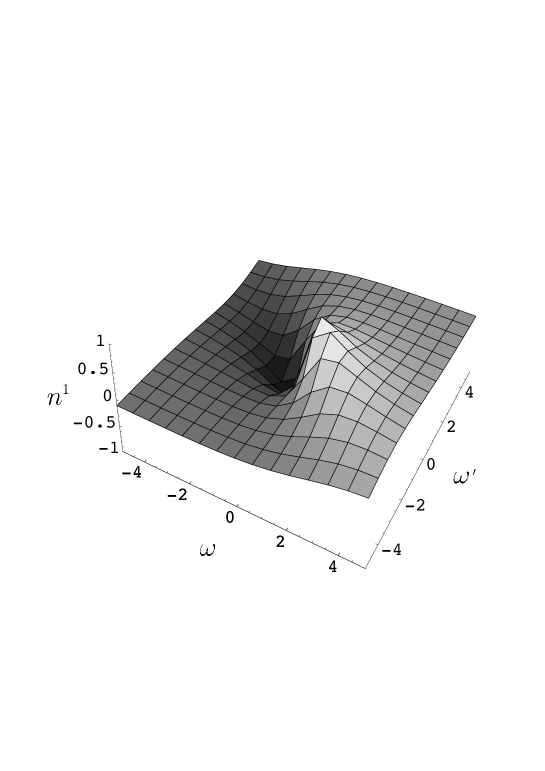
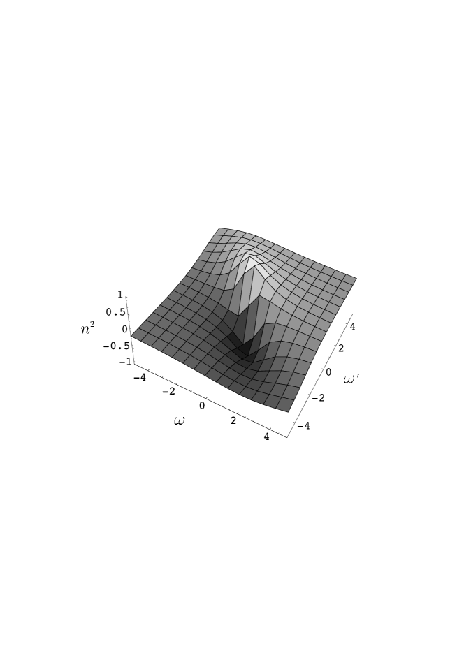
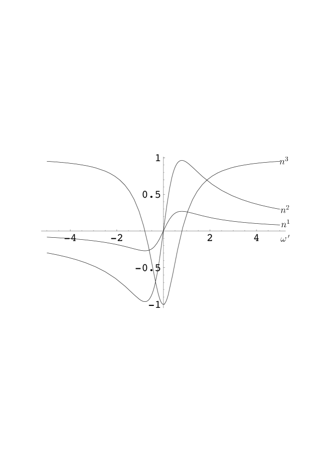
V numerical investigation of a special case

To understand the behaviour of $\bm{n}$, we here consider the following specific case:

$$k=(k_{0},k_{0},0,0),\hskip 5.69054ptl=(l_{0},0,l_{0},0),\hskip 5.69054ptl=(m_{0},0,0,m_{0}),$$

$$P=Q=1,\hskip 5.69054ptR=0,$$

$$u_{0}=1,\hskip 5.69054ptv_{0}=-1.$$ (131)

Then we have

$$\kappa^{1}=\sqrt{\frac{c_{4}}{c_{2}}}\hskip 2.84526ptk_{0},\hskip 5.69054pt\kappa^{2}=\sqrt{\frac{c_{4}}{c_{2}}}\hskip 2.84526ptl_{0},\hskip 5.69054pt\kappa^{3}=\sqrt{\frac{c_{4}}{c_{2}}}\hskip 2.84526ptm_{0},$$

$$\xi=\sqrt{\frac{c_{2}}{c_{4}}}(x_{0}-x_{1}),\hskip 5.69054pt\eta=\sqrt{\frac{c_{2}}{c_{4}}}(x_{0}-x_{2}),\hskip 5.69054pt\zeta=\sqrt{\frac{c_{2}}{c_{4}}}(x_{0}-x_{3}).$$ (132)

In this case, the variables $\omega$ and $\omega^{\prime}$ are independent of the time variable $x_{0}$:

$$\omega=\sqrt{\frac{c_{2}}{c_{4}}}(-2x_{1}+x_{2}+x_{3}),$$ (133)

$$\omega^{\prime}=\sqrt{\frac{c_{2}}{c_{4}}}(-x_{2}+x_{3}).$$ (134)

We also specify the functions $\psi(z)$ and $F(u_{1}+iv_{1})$ as

$$\psi(z)=z^{2},$$ (135)

$$F(u_{1}+iv_{1})=u_{1}+iv_{1}.$$ (136)

Then we have

$$\rho=\frac{1}{\sqrt{5}}$$ (137)

$$u=u_{1}=\frac{1}{49}[(51+2\sqrt{5})\omega+(39-10\sqrt{5})\omega^{\prime}],$$ (138)

$$v=v_{1}=\frac{1}{49}[(34-3\sqrt{5})\omega+(26+15\sqrt{5})\omega^{\prime}].$$ (139)

and

$$|f|^{2}=u^{2}+v^{2}=\frac{26}{49}(3\omega^{2}+4\omega\omega^{\prime}+3\omega^{\prime 2}).$$ (140)

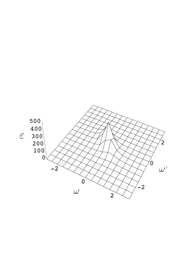
The static energy density

$$E=4c_{2}\frac{\nabla f\cdot\nabla f^{*}}{(1+|f|^{2})^{2}}-4c_{4}\frac{(\nabla f\times\nabla f^{*})^{2}}{(1+|f|^{2})^{4}}$$ (141)

turns out to be

$$E=\frac{c_{2}^{2}}{c_{4}}\varepsilon,$$

$$\varepsilon=\frac{4(\delta_{1}+\delta_{2})}{(1+|f|^{2})^{2}}+\frac{16(\delta_{1}\delta_{2}-\delta_{3}^{2})}{(1+|f|^{2})^{4}},$$ (142)

where $\delta_{1}$, $\delta_{2}$ and $\delta_{3}$ are given by

$$\delta_{1}=6\biggl{(}\frac{\partial u_{1}}{\partial\omega}\biggr{)}^{2}+2\biggl{(}\frac{\partial u_{1}}{\partial\omega^{\prime}}\biggr{)}^{2}=\frac{8(353-6\sqrt{5})}{343},$$ (143)

$$\delta_{2}=6\biggl{(}\frac{\partial v_{1}}{\partial\omega}\biggr{)}^{2}+2\biggl{(}\frac{\partial v_{1}}{\partial\omega^{\prime}}\biggr{)}^{2}=\frac{8(193+6\sqrt{5})}{343},$$ (144)

$$\delta_{3}=6\frac{\partial u_{1}}{\partial\omega}\frac{\partial v_{1}}{\partial\omega}+2\frac{\partial u_{1}}{\partial\omega^{\prime}}\frac{\partial v_{1}}{\partial\omega^{\prime}}=\frac{4(384+5\sqrt{5})}{343},$$ (145)

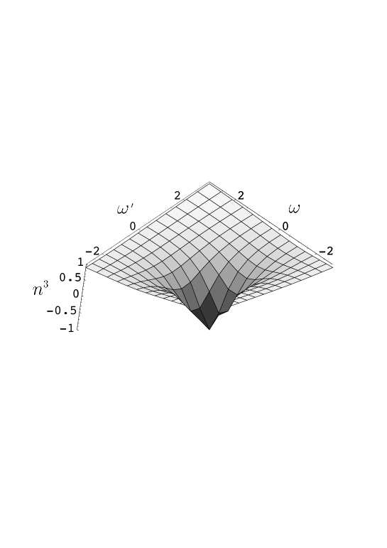
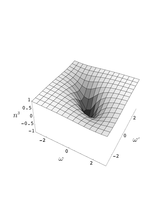
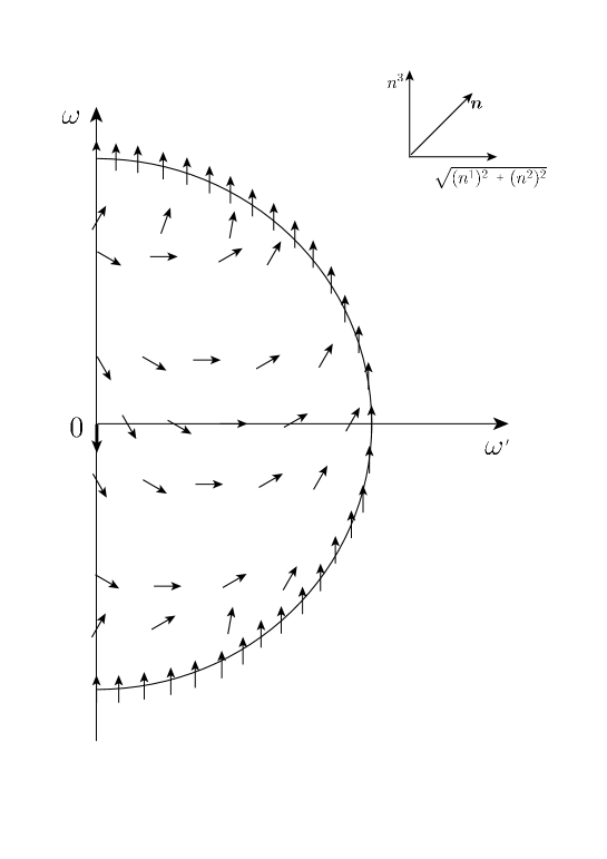
We see that $\bm{n}$ is equal to $(0,0,-1)$ at $(\omega,\omega^{\prime})=(0,0)$ and that $\bm{n}$ approaches to $(0,0,1)$ as $|\omega|$ and $|\omega^{\prime}|$ increase. In Figs.1, 2, 3, 4 and 5, the behaviour of $\bm{n}$ is shown. In Fig.6, the direction of $\bm{n}$ is shown schematically. In Fig.7, the behaviour of $\varepsilon$ is shown. As is seen from Eqs. (133) and (134), the ($\omega$, $\omega^{\prime}$)-plane can be regarded as a plane with the normal $(1,1,1)/\sqrt{3}$ in the physical $(x_{1},x_{2},x_{3})$-plane.

VI Summary and discussion

In this paper, we have clarified the interrelation between the Skyrme model for the matrix field $g(x)\in SU(2)$ and the Faddeev model for the isovector scalar field $\bm{n}(x)\in S^{2}$. By comparing the vector field descriptions making use of $\bm{A}_{\mu}=\frac{1}{2i}\text{tr}(\bm{\tau}g^{\dagger}\partial_{\mu}g)$ and $\bm{B}_{\mu}=\bm{n}\times\partial_{\mu}\bm{n}$, it was concluded that the Faddeev model can be regarded as the mesonic sector of the Skyrme model in which the baryon number current vanishes everywhere.

Next, we have explored the exact solutions of the Faddeev model. Under the Ansatz that $\bm{n}(x)$ is a function of the variables $k\cdot x$, $l\cdot x$ and $m\cdot x$ with $k$, $l$ and $m$ being Minkowskian lightlike 4-vectors, the field equation for $\bm{B}_{\mu}$ has been reduced to the nonlinear differential equation (24) for the isovector scalar fields $\bm{a}$, $\bm{b}$ and $\bm{c}$. From the assumption (25) which ensures the condition (14), We have seen that $\bm{a}$,$\bm{b}$ and $\bm{c}$ should depend only on the two variables $\omega$ and $\omega^{\prime}$. We have seen that the field equation for $\bm{n}$ can be rewritten as the coupled equations (54), (55) and (44) for the scalars $\kappa$, $\lambda$, $\mu$ and $\nu$ defined by Eqs. (40), (41), (42) and (43). Restricting ourselves to the case of vanishing $\nu$, the above equations have been reduced to the tractable system of equations (58) and (59) for $\lambda$ and $\mu$. We have found that these equations can be reduced to the nonlinear equation (63) for $J(\omega,\omega^{\prime})$, which has the solution (77) involving one arbitrary function $\psi(z)$. The restriction (85) has led us to the generalized Cauchy-Riemann relation (88), which has been solved in terms of an arbitrary analytic function $F(u_{1}+iv_{1})$ where $u_{1}$ and $v_{1}$ are given by (102) and (103). Thus, roughly speaking, the field equation of the Faddeev model has been solved under the assumptions (15), (25) and (56). We have pointed out that $u$ and $v$ in the $\nu=0$ case can be interpreted as a pair of isothermal coordinates of a Riemannian surface. Our solutions of the Faddeev model involve arbitrary lightlike 4-momenta $k$, $l$ and $m$, arbitrary parameters $P$, $Q$, $R$, $u_{0}$ and $v_{0}$, an arbitrary function $\psi(z)$, and an arbitrary analytic function $F(u_{1}+iv_{1})$.

As an example of a numerical estimation, we have considered the simplest case $P=1$, $Q=1$, $R=0$, $u_{0}=-v_{0}=1$, $\psi(z)=z^{2}$ and $F(u_{1}+iv_{1})=u_{1}+iv_{1}$ and found the static vortex solution in which $\bm{n}=(0,0,-1)$ at $(\omega,\omega^{\prime})=(0,0)$ and $\bm{n}=(0,0,1)$ for large $\omega^{2}+{\omega^{\prime}}^{2}$. If we define the topological charge $\Phi$ by

$$\Phi=\frac{1}{4\pi}\int_{-\infty}^{\infty}d\omega\int_{-\infty}^{\infty}d\omega^{\prime}\bm{n}\cdot\biggl{(}\frac{\partial\bm{n}}{\partial\omega}\times\frac{\partial\bm{n}}{\partial\omega^{\prime}}\biggr{)},$$ (146)

$\Phi$ is given by

$$\Phi=-mn,$$ (147)

where $m$ and $n$ are the winding numbers of the two mappings $(\omega,\omega^{\prime})\rightarrow(u_{1},v_{1})$ and $(u_{1},v_{1})\rightarrow(u,v)$, respectively. The former mapping is governed by the arbitrary function $\rho(z)$, while the latter by the arbitrary analytic function $F(u_{1}+iv_{1})$.

We hope our method gives some hints to obtain the analytic expressions of the knot solutions in Battye found by numerical investigations . Since $\bm{n}$ appears in the description of Yang-Mills field Cho ; Morita ; Faddeevn , the vortex structure of $\bm{n}$ observed here might suggest the same structure of the Yang-Mills field. We should note that the existence of the vortex solution of the Faddeev model was also discussed by Kundu and Rybakov KunduRy . We finally note that, although no exact analytic expression was presented, the vortex solution of the Abelian Higgs model was found by Nielsen and Olesen Nielsen thirty years ago.

Figure 1: The behaviour of $n^{1}(\omega,\omega^{\prime})$.

Figure 2: The behaviour of $n^{2}(\omega,\omega^{\prime})$.

Figure 3: The behaviour of $n^{3}(\omega,\omega^{\prime})$ looked at from the bottom.

Figure 4: The behaviour of $n^{3}(\omega,\omega^{\prime})$ looked at from the top.

Figure 5: The behaviours of $n^{1}(\omega,\omega^{\prime})$, $n^{2}(\omega,\omega^{\prime})$ and $n^{3}(\omega,\omega^{\prime})$ for $\omega=0$.

Figure 6: The schematic description of the direction of $\bm{n}(\omega,\omega^{\prime})$.

Figure 7: The behaviour of $\varepsilon(\omega,\omega^{\prime})$.