Light-Cone String Field Theory in a Plane Wave

Abstract

These lecture notes present an elementary introduction to light-cone string field theory, with an emphasis on its application to the study of string interactions in the plane wave limit of AdS/CFT. We summarize recent results and conclude with a list of open questions.

1 Introduction

1.1 Light-Cone String Field Theory

These lectures are primarily about light-cone string field theory, which is an ancient subject (by modern standards) whose origins lie in the days of ‘dual resonance models’ even before string theory was studied as a theory of quantum gravity [1, 2, 3, 4, 8, 9, 10]. Light-cone string field theory is nothing more than the study of string theory (especially string interactions) via Hamiltonian quantization in light-cone gauge. Let us immediately illustrate this point.

Textbooks on string theory typically begin by considering the Polyakov action for a free string,

$$S={1\over 4\pi\alpha^{\prime}}\int_{\Sigma}\sqrt{\gamma}\gamma^{\alpha\beta}\partial_{\alpha}X^{\mu}{\partial}_{\beta}X_{\mu}+\mbox{fermions}+\mbox{ghosts},$$ (1)

where $\Sigma$ is the $1+1$-dimensional string worldsheet (we consider only closed strings in these lectures), $\gamma$ is the metric on $\Sigma$, and $X^{\mu}$ is the embedding of the string worldsheet into spacetime. Quantizing this theory is simplest in light-cone gauge, where the ghosts are not needed, and one finds the light-cone Hamiltonian

$$H=2p^{-}={1\over p^{+}}\left[{1\over 2}p^{i}p^{i}+{1\over\alpha^{\prime}}\sum_{n=1}^{\infty}(\alpha_{-n}^{i}\alpha_{n}^{i}+\tilde{\alpha}_{-n}^{i}\tilde{\alpha}_{n}^{i})+\mbox{fermions}\right],$$ (2)

where $i$ labels the directions transverse to the light-cone. At this stage most textbooks abandon light-cone gauge in favor of more powerful and mathematically beautiful covariant techniques.

However, it is also possible to continue by second-quantizing (or third-quantizing, depending on how you count) the Hamiltonian (2). To do this we introduce a multi-string Hilbert space, with operators acting to create or annihilate entire strings (not to be confused with the operators $\alpha_{n}^{i}$ and $\tilde{\alpha}_{n}^{i}$, which create or annihilate an oscillation of frequency $n$ on a given string). All of the details will be presented in Lecture 2, where our ultimate goal will be to write down a relatively simple interaction term which (at least for the bosonic string) is able to reproduce (in principle) all possible string scattering amplitudes!

Light-cone string field theory obscures many important properties of string theory which are manifest in a covariant treatment. Nevertheless, the subject has recently enjoyed a remarkable renaissance following [39] because it is well-suited for studying string interactions in a maximally symmetric plane wave background, where covariant techniques are more complicated than they are in flat space.

1.2 The Plane Wave Limit of AdS/CFT

One of the most exciting developments in string theory has been the discovery of the AdS/CFT correspondence [20] (see [23] for a review). The best understood example of this correspondence relates type IIB string theory on $AdS_{5}\times S^{5}$ to SU($N$) Yang-Mills theory with ${\cal{N}}=4$ supersymmetry. Although we have learned a tremendous amount about gauge theory, quantum gravity, and the holographic principle from AdS/CFT, the full promise of the duality has unfortunately not yet been realized. The reason is simple: string theory on $AdS_{5}\times S^{5}$ is hard!

In contrast to (1), the Green-Schwarz superstring on $AdS_{5}\times S^{5}$ is nontrivial. It can be regarded as a coset sigma model on $PSU(2,2|4)/SO(4,1)\times SO(5)$ with an additional fermionic Wess-Zumino term and a fermionic $\kappa$-symmetry [21, 22, 24]. Despite some intriguing recent progress [96, 108], this theory remains intractable and we still do not know the free string spectrum (i.e., the analogue of (2)) in $AdS_{5}\times S^{5}$. Because of this difficulty, most applications of the AdS/CFT correspondence rely on the supergravity approximation to the full string theory.

Recently, a third maximally symmetric 10-dimensional solution of type IIB string theory was found [25, 27]: the so-called maximally symmetric plane wave background. This background can be obtained from $AdS_{5}\times S^{5}$ by taking a Penrose limit, and it is essentially flat space plus the first order correction from flat space to the full $AdS_{5}\times S^{5}$. In some sense this background sits half-way between flat space and $AdS_{5}\times S^{5}$. It resembles $AdS_{5}\times S^{5}$ because it is a curved geometry with non-zero five-form flux, and it resembles flat space because remarkably, the free string theory in this background can be solved exactly in light-cone gauge [26] (the details will be presented in Lecture 1).

Furthermore it was realized in [29] that the Penrose limit of $AdS_{5}\times S^{5}$ has a very simple description in terms of the dual Yang-Mills theory. In particular, BMN related IIB string theory on the plane wave background to a sector of the large $N$ limit of ${\cal{N}}=4$ SU($N$) gauge theory involving operators of large R-charge $J\sim\sqrt{N}$.

Because string theory in the plane wave is exactly solvable, the BMN correspondence opens up the exciting opportunity to study stringy effects in the holographic dual gauge theory, thereby adding a new dimension to our understanding of gauge theory, gravity, and the holographic principle. Light-cone string field theory, although somewhat esoteric, has emerged from a long hibernation because it naturally connects the string and gauge theory descriptions of the plane wave limit of AdS/CFT.

1.3 What is and what is not in these Notes

Light-cone string field theory is a very complicated and technical subject. In order to provide a pedagogical introduction, most of the material is developed for the simpler case of the bosonic string, although we do mention the qualitatively new features which arise for the type IIB string. The reader who is interested in a detailed study of the latter, significantly more complicated case is encouraged to refer to the papers [39, 50, 73], or to review articles such as [105, 103]. Our goal here has been to present in a clear manner the relevant background material which is usually absent in the recent literature on plane waves.

2 Lecture 1: The Plane Wave Limit of AdS/CFT

2.1 Lightning Review of the AdS/CFT Correspondence

We start with a quick review of the remarkable duality between ${\cal{N}}=4$ SU($N$) super-Yang Mills theory and type IIB string theory on $AdS_{5}\times S^{5}$, referring the reader to [23] for an extensive review and for additional references. This is the best understood and most concrete example of a holographic duality between gauge theory and string theory.

The Lagrangian for ${\cal{N}}=4$ super-Yang Mills theory is [28]

$${\cal{L}}={\rm Tr}\left[-{1\over 2g_{\rm YM}^{2}}F_{\mu\nu}F^{\mu\nu}-{1\over 2}\sum_{i}D_{\mu}\phi^{i}D^{\mu}\phi^{i}+{g_{\rm YM}^{2}\over 4}\sum_{i,j}[\phi^{i},\phi^{j}]^{2}+{\rm fermions}\right],$$ (3)

where $F_{\mu\nu}$ is the gauge field strength and $\phi^{i}$, $i=1,\ldots,6$ are six real scalar fields. All fields transform in the adjoint representation of the gauge group. The ${\cal{N}}=4$ superalgebra in four dimensions is very constraining and essentially determines the field content and the Lagrangian (3) uniquely: the only freedom is the choice of gauge group (which will always be SU($N$) in these lectures), and the value of the coupling constant $g_{\rm YM}$. This theory is conformally invariant, so $g_{\rm YM}$ is a true parameter of the theory. (In non-conformal theories, couplings become functions of the energy scale, rather than parameters.) The symmetry of the Lagrangian (3) is SO(2,4)$\times$SO(6), where the first factor is the conformal group in four dimensions and the second group is the SO(6) R-symmetry group which acts on the six scalar fields in the obvious way.

On the other side of the duality we have type IIB string theory on the $AdS_{5}\times S^{5}$ spacetime, whose metric can be written as

$$ds^{2}={r^{2}\over R^{2}}(-dx_{0}^{2}+dx_{1}^{2}+dx_{2}^{2}+dx_{3}^{2})+R^{2}{dr^{2}\over r^{2}}+R^{2}d\Omega_{5}^{2}.$$ (4)

This is a solution of the IIB equations of motion with constant string coupling $g_{s}$ and five-form field strength

$$F_{5}=(1+*)dx_{0}\wedge dx_{1}\wedge dx_{2}\wedge dx_{3}\wedge d(R^{4}/r^{4}).$$ (5)

The isometry group of the spacetime is SO(2,4)$\times$SO(6), where the first factor is the isometry of $AdS_{5}$ and the second factor is the isometry of $S^{5}$.

According to the AdS/CFT correspondence, there is a one-to-one correspondence between single-trace operators ${{O}}$ in the gauge theory and fields $\phi$ in AdS. The holographic dictionary between the two sides of this duality is summarized in Table 1, where $\lambda=g_{\rm YM}^{2}N$ is the ’t Hooft coupling and $\sqrt{\alpha^{\prime}}$ is the string length.

${\cal{N}}=4$ SU($N$) super-Yang Mills	$\Longleftrightarrow$	IIB string theory on $AdS_{5}\times S^{5}$
$g_{\rm YM}^{2}$	$=$	$4\pi g_{s}$
$\lambda^{1/4}=(g_{\rm YM}^{2}N)^{1/4}$	$=$	$R/\sqrt{\alpha^{\prime}}$
$\left<\exp\left[\int d^{4}x\ \phi_{0}(x){{O}}(x)\right]\right>_{\rm CFT}$	$=$	$Z_{\rm string}\left[\left.\phi(x,r)\right|_{r=0}=\phi_{0}(x)\right]$

Table 1: The AdS/CFT correspondence for $AdS_{5}\times S^{5}$.

2.2 The Penrose Limit of $AdS_{5}\times S^{5}$

Now we consider a particular limit (a special case of a Penrose Limit) of the $AdS_{5}\times S^{5}$ background, following the treatment in [29]. The limit we consider can be thought of as focusing very closely upon the neighborhood of a particle which is sitting in the ‘center’ of $AdS_{5}$ and moving very rapidly (close to the speed of light) along the equator of the $S^{5}$. To this end it is convenient to write the $AdS_{5}\times S^{5}$ metric in the following coordinate system:

$${ds^{2}\over R^{2}}=\underbrace{-dt^{2}\cosh^{2}\rho+d\rho^{2}+\sinh^{2}\rho d\Omega_{3}^{2}}_{AdS_{5}}+\underbrace{d\psi^{2}\cos^{2}\theta+d\theta^{2}+\sin^{2}\theta d\Omega_{3}^{\prime 2}}_{S^{5}}.$$ (6)

Now $\rho=0$ is the ‘center’ of $AdS_{5}$ and $\rho=\infty$ is the boundary. (These are respectively $r=\infty$ and $r=0$ in the coordinate system of (4)). The coordinate $\theta\in[-{\pi\over 2},{\pi\over 2}]$ is the ‘latitude’ on the $S^{5}$ and $\psi$, which is periodic modulo $2\pi$, is the coordinate along the equator of the $S^{5}$.

Note that by singling out an equator along the $S^{5}$, we have broken the manifest SO(6) isometry of the metric on $S^{5}$ down to U(1)$\times$SO(4).

Now consider the coordinates $\widetilde{x}^{\pm}={1\over 2}(t\pm\psi)$, which are appropriate for a particle traveling along the trajectory $t-\psi\approx 0$. To focus in on the neighborhood of this particle, which is sitting at $\rho=\theta=0$, means to consider the following range of coordinates:

$$\widetilde{x}^{+}={\rm finite},\qquad\widetilde{x}^{-}={\rm infinitesimal},\qquad\rho={\rm infinitesimal},\qquad y={\rm infinitesimal}.$$ (7)

In order to isolate this range of coordinates, it is convenient to rescale the coordinates according to

$$x^{+}=\widetilde{x}^{+},\qquad x^{-}=R^{2}\widetilde{x}^{-},\qquad\rho={r\over R},\qquad\theta={y\over R}$$ (8)

and then take the limit $R\to\infty$. Taking this limit of (6) brings the metric into the form

$$ds^{2}=-4dx^{+}dx^{-}-(r^{2}+y^{2})(dx^{+})^{2}+dr^{2}+r^{2}d\Omega_{3}^{2}+dy^{2}+y^{2}d\Omega_{3}^{\prime 2}.$$ (9)

The last four terms are just the flat metric on ${\mathbb{R}}^{4}\times{\mathbb{R}}^{4}={\mathbb{R}}^{8}$, so we can rewrite the metric more simply as

$$ds^{2}=-4dx^{+}dx^{-}-\mu^{2}x^{2}(dx^{+})^{2}+dx_{I}dx^{I},$$ (10)

where $I=1,\ldots,8$. In this formula we have introduced a new parameter $\mu$. Note that $\mu$ is essentially irrelevant since it can always be eliminated by a Lorentz boost in the $x^{+}$–$x^{-}$ plane, $x^{\pm}\to x^{\pm}\mu^{\pm 1}$. However, $\mu$ will serve as a useful bookkeeping device.

We should not forget about the five-form field strength (5), which remains non-zero in the Penrose limit of the $AdS_{5}\times S^{5}$ solution. Taking the appropriate limit of (5) gives

$$F_{+1234}=F_{+5678}={\mu\over 4\pi^{3}g_{s}\alpha^{\prime 2}}.$$ (11)

The metric (10) and five-form (11) themselves constitute the maximally symmetric plane wave (‘pp-wave’) solution of the equations of motion of type IIB string theory. Note that the full symmetry of this background is SO(4)$\times$SO(4)$\times{\mathbb{Z}}_{2}$. The first SO(4) is a remnant of the SO(2,4) isometry group of $AdS_{5}$ and the second SO(4) is a remnant of the SO(6) isometry group of $S^{5}$. The ${\mathbb{Z}}_{2}$ symmetry exchanges these two SO(4)’s, acting on the coordinates $x^{i}$ by $(x_{1},x_{2},x_{3},x_{4})\leftrightarrow(x_{5},x_{6},x_{7},x_{8})$. This peculiar discrete symmetry survives only in the strict pp-wave limit. This symmetry is broken if we perturb slightly away from the limit back to $AdS_{5}\times S^{5}$.

In summary: we started with the $AdS_{5}\times S^{5}$ solution of IIB string theory, and we took a limit which focused on the neighborhood around a trajectory traveling very rapidly around the equator of the $S^{5}$, and we arrived at a different solution of IIB string theory. The natural question is now: what does this Penrose limit correspond to on the gauge theory side of the AdS/CFT correspondence?

First, note that since we had to break the SO(6) symmetry of the $S^{5}$ by choosing an equator, then on the gauge theory side we must also break the SO(6) symmetry to SO(4)$\times$U(1) by choosing some U(1) subgroup of the R-symmetry group. Without loss of generality we can choose this U(1) subgroup to be the group of rotations in the $\phi^{5}$–$\phi^{6}$ plane. From now on, when we talk about the R-charge of some state, we mean the charge of the state with respect to this U(1) subgroup of the full R-symmetry group.

Next, it is useful to trace through the above coordinate transformations to see what the light-cone energy $p^{-}$ and light-cone momentum $p^{+}$ correspond to on the gauge theory side. To this end, recall that the energy in global coordinates in $AdS_{5}$ is given by $E=i\partial_{t}$ and the angular momentum (around the equator of the $S^{5}$) is $J=-i\partial_{\psi}$. In terms of the dual CFT, these correspond respectively to the conformal dimension $\Delta$ and R-charge of an operator. Therefore we obtain the identification:

$$2p^{-}=-p_{+}=i\partial_{x^{+}}=i\partial_{\widetilde{x}^{+}}=i(\partial_{t}+\partial_{\psi})=\Delta-J,$$ (12)

$$2p^{+}\equiv-p_{-}=-{\widetilde{p}_{-}\over R^{2}}={1\over R^{2}}i\partial_{\widetilde{x}^{-}}={1\over R^{2}}i(\partial_{t}-\partial_{\psi})={\Delta+J\over R^{2}}.$$ (13)

On the string theory side, when we say that we ‘focus in on’ a small neighborhood of the equatorial trajectory, what that means is that we consider amongst all the possible fluctuations of IIB string theory on $AdS_{5}\times S^{5}$ only those which are localized in that small neighborhood. Now (12) and (13) suggest that on the gauge theory side, this truncation corresponds to considering those operators which have finite $\Delta-J$, and $\Delta+J\sim R^{2}\sim\sqrt{N}$. Therefore we arrive at the so-called BMN correspondence, as summarized in Table 2.

${\cal{N}}=4$ SU($N$) super-Yang Mills,	$\Longleftrightarrow$	IIB string theory on $AdS_{5}\times S^{5}$,
in the limit $N\to\infty$, $g_{\rm YM}=$ fixed,		in the limit $R\to\infty$, $g_{s}=$ fixed,
truncated to operators with		truncated to states with
$\Delta\sim J\sim\sqrt{N}$ and finite $\Delta-J$		finite $p^{+}$ and $p^{-}$
$||$		$||$
?		IIB string theory on a plane wave
$\Delta-J$	$=$	${2\over\mu}p^{-}$
$J/\sqrt{\lambda}$	$=$	$\mu p^{+}\alpha^{\prime}$

Table 2: The plane wave limit of the AdS/CFT correspondence.

It will be very convenient to define the quantities

$$\lambda^{\prime}={g_{\rm YM}^{2}N\over J^{2}}={1\over(\mu p^{+}\alpha^{\prime})^{2}},\qquad g_{2}={J^{2}\over N}$$ (14)

which remain finite in the BMN limit. Also, we will refer to those operators with $\Delta\sim J\sim\sqrt{N}$ and finite $\Delta-J$ as ‘BMN operators’.

In Table 2 we have introduced the parameter $\mu$ by rescaling $x^{\pm}$ as discussed above. The question mark in Table 2 indicates that we are still looking for a nice way to characterize this limit of the gauge theory. In other words, what precisely does it mean to ‘truncate’ the theory to a certain class of operators; or, turned around: is there a simple description of the sector of the gauge theory which is dual to IIB string theory on a plane wave?

2.3 Strings on Plane Waves

The most exciting aspect of the BMN correspondence is that the free IIB string on the plane wave background is exactly solvable. As discussed in the introduction, string theory on $AdS_{5}\times S^{5}$ is in contrast rather complicated.

In light cone gauge, the worldsheet theory for IIB strings on the plane wave background (Green-Schwarz action) is simply [26]

$$S={1\over 2\pi\alpha^{\prime}}\int dt\int_{0}^{2\pi\alpha^{\prime}p^{+}}d\sigma\left[{1\over 2}\dot{X}^{2}-{1\over 2}X^{\prime 2}-{1\over 2}\mu^{2}X^{2}+i\overline{S}(\partial\!\!\!/+\mu\Pi)S\right],$$ (15)

where $X^{I}$, $I=1,\ldots,8$ are the bosonic sigma model coordinates, $S$ is a complex Majorana spinor on the worldsheet and a positive chirality SO(8) spinor under rotations in the transverse directions, and $\Pi=\Gamma^{1}\Gamma^{2}\Gamma^{3}\Gamma^{4}$.

The action (15) simply describes eight massive bosons and eight massive fermions, so it is trivially solvable. Let us consider here only bosonic excitations. Then a general state has the form

$$a_{n_{1}}^{I_{1}}\cdots a_{n_{m}}^{I_{m}}|0;p^{+}\rangle,$$ (16)

and the Hamiltonian be written as

$$2p^{-}=-p_{+}=\sum_{n=-\infty}^{\infty}\sum_{I=1}^{8}(a_{n}^{I})^{\dagger}a_{n}^{I}\sqrt{\mu^{2}+{n^{2}\over(\alpha^{\prime}p^{+})^{2}}}.$$ (17)

We have chosen a basis of Fourier modes such that $n>0$ label left movers, $n<0$ label right movers, and $n=0$ is the zero mode. This convention has become standard in the pp-wave literature and contrasts with the usual convention in flat space, where the left- and right-moving oscillators are denoted by different symbols $\alpha_{n}$ and $\tilde{\alpha}_{n}$.

The alternate convention can be motivated by recalling that in flat space, the worldsheet theory remains a conformal field theory even in light-cone gauge. Therefore the left-moving modes $\alpha_{n}$ and the right-moving modes $\tilde{\alpha}_{n}$ decouple from each other. However, in the plane-wave background, choosing light-cone gauge breaks conformal invariance on the world sheet (because a mass term appears). Therefore all of the modes couple to each other, so there is no advantage to introducing a notation which treats left- and right-movers separately.

Since this is a theory of closed strings, we should not forget to impose the physical state condition, which says that the total momentum on the string should vanish:

$$P=\sum_{n=-\infty}^{\infty}\sum_{I=1}^{8}nN^{I}_{n}=0,$$ (18)

where $N^{I}_{n}$ is the occupation number (the eigenvalue of $(a_{n}^{I})^{\dagger}a_{n}^{I}$).

We remarked above that the SO(8) transverse symmetry is broken by the five-form field strength to SO(4)$\times$SO(4)$\times{\mathbb{Z}}_{2}$. This manifests itself by the presence of $\Pi$ in the worldsheet action (15). However, the free spectrum of IIB string theory on the plane wave is actually fully SO(8) symmetric [69]. One can see this by noting that $\Pi$ can be eliminated from (15) by first splitting $S=S_{1}+iS_{2}$ and then making the field redefinition $S_{2}\to\Pi S_{2}$. One should think of SO(8) as an accidental symmetry of the free theory. Since the background breaks SO(8) to SO(4)$\times$SO(4)$\times{\mathbb{Z}}_{2}$, there is no reason to expect that string interactions should preserve the full SO(8), and indeed we will see that they do not: the interactions break SO(8) to SO(4)$\times$SO(4)$\times{\mathbb{Z}}_{2}$.

Before we return to the gauge theory, it will be convenient to rewrite the spectrum (17) in terms of gauge theory parameters using the dictionary from Table 2:

$$\Delta-J=\sum_{n}\sum_{I=1}^{8}N^{I}_{n}\sqrt{1+\lambda^{\prime}n^{2}}.$$ (19)

2.4 Strings from ${\cal{N}}=4$ Super Yang Mills

We have seen that IIB string theory on the plane wave background has a very simple spectrum (19). In this section we will recover this spectrum by finding the set of operators which have $\Delta\sim J\sim\sqrt{N}$ and finite $\Delta-J$ in the $N\to\infty$ limit [29].

Consider first the ground state of the string, $|0;p^{+}\rangle$. According to (19) this should correspond to an operator with $\Delta-J=0$. The unique such operator is ${\rm Tr}[Z^{J}]$, where

$$Z={1\over\sqrt{2}}(\phi_{5}+i\phi_{6})$$ (20)

(recall that we defined $J$ to be the U(1) generator which acts by rotation in the $\phi_{5}$–$\phi_{6}$ plane). The first entry in the ‘BMN state-operator correspondence’ is therefore

$$|0;p^{+}\rangle\qquad\Longleftrightarrow\qquad{\rm Tr}[Z^{J}].$$ (21)

To get the first excited states we can add to the trace operators which have $\Delta-J=1$; for example: $\phi_{i}$ (for $i=1,2,3,4$) or $D_{i}Z$ (again for $i=1,2,3,4$, in the Euclidean theory).

$$a_{0}^{i}|0;p^{+}\rangle \Longleftrightarrow {\rm Tr}[\phi_{i}Z^{J}],$$ (22)

$$a_{0}^{i+4}|0;p^{+}\rangle \Longleftrightarrow {\rm Tr}[D_{i}ZZ^{J}].$$ (23)

To get higher excited states we can add more ‘impurities’ to the traces. For example, a general state with $\Delta-J=k$ is

$$a_{0}^{i_{1}}a_{0}^{i_{2}}\cdots a_{0}^{i_{k}}|0;p^{+}\rangle\Longleftrightarrow\sum{\rm Tr}[\cdots Z\phi_{i_{1}}Z\cdots Z\phi_{i_{k}}Z\cdots].$$ (24)

The sum on the right hand side runs over all possible orderings of the insertions inside the trace. This sum is necessary to ensure that the operator is BPS. We will always work in a ‘dilute gas’ approximation, where the number of impurities is much smaller than $J$, the number of $Z$’s.

So far we considered only BPS operators in the gauge theory. These have the property that $\Delta$ is not corrected by interactions, i.e. $\Delta$ does not depend on $g_{\rm YM}$. According to (19), these can only correspond to string states with the zero mode ($n=0$) excited. In order to obtain other states, we can consider summing over the location of an impurity with a phase:

$$a_{n}^{i}|0;p^{+}\rangle\qquad\Longleftrightarrow\qquad\sum_{k=0}^{J}e^{2\pi ink/J}{\rm Tr}[Z^{k}\phi_{i}Z^{J-k}].$$ (25)

But the right hand side is zero (for $n\neq 0$), because of cyclicity of the trace! Actually this is a good thing, because the string state on the left does not satisfy the physical state condition for $n\neq 0$.

In order to get physical states, we have to consider (suppressing the $i$ transverse index)

$$a_{n_{1}}\cdots a_{n_{m}}|0;p^{+}\rangle\Longleftrightarrow\sum_{k_{1},\ldots,k_{m}=0}^{J}e^{2\pi i(n_{1}k_{1}+\cdots+n_{m}k_{m})/J}{\rm Tr}[\cdots Z\phi Z\cdots Z\phi Z\cdots].$$ (26)

Here $k_{i}$ labels the position, in the string of $Z$’s, of the $i$-th $\phi$ impurity. Cyclicity of the trace now implies that the right-hand side vanishes unless $n_{1}+\cdots+n_{m}=0$, and this is precisely the physical state condition for the string state on the left-hand side!

The operator on the right-hand side of (26) is not BPS when the phases are non-zero, so its dimension $\Delta$ receives quantum corrections. One can check that in the BMN limit $N,J\to\infty$ with $J\sim\sqrt{N}$, the contribution to $\Delta-J$ from an impurity with phase $n$ is

$$(\Delta-J)_{n}=\sqrt{1+\lambda^{\prime}n^{2}},$$ (27)

precisely in accord with the prediction (19)! This calculation was performed to one loop in [29], to two loops in [62], and an argument valid to all orders in perturbation theory was presented in [51].

At this point we have motivated that the spectrum of IIB string theory on the plane wave background can be identified with the set of BMN operators in ${\cal{N}}=4$ SU($N$) Yang-Mills theory. One point which we did not consider is the addition of impurities with $\Delta-J>1$, for example $\overline{Z}$, which has $\Delta-J=2$. It has been argued that these operators decouple in the BMN limit (i.e., their anomalous dimensions go to infinity), and can hence be ignored. We refer the reader to [29] for details. Next we present the two parameters [40, 43] which characterize the BMN limit.

2.5 The Effective ’t Hooft Coupling $\lambda^{\prime}$

Something a little miraculous has happened. The operator (26) is not BPS (when the phases are nonzero), so its conformal dimension $\Delta$ will receive quantum corrections. Generically, the dimension of a non-protected operator blows up in limit of large ’t Hooft coupling. And we certainly are taking $\lambda=g_{\rm YM}^{2}N\to\infty$ here (see Table 2)!

However, note that (26) is BPS when all of the phases are zero: $n_{1}=\cdots=n_{m}=0$. In a sense, then, we might hope that the operator is ‘almost’ BPS as long as the phases are almost 0, or in other words $n_{i}/J\ll 1$ for all $i$. By ‘almost’ BPS we mean that although the dimension does receive quantum corrections, those corrections are finite in the BMN limit despite the fact that $\lambda\to\infty$. Indeed this is what happens: in the formula (19) is it not the ‘t Hooft coupling $\lambda$ which appears, but rather a new effective coupling $\lambda^{\prime}=\lambda/J^{2}$ which is finite in the BMN limit.

It is hoped (and indeed this hope is borne out in all known calculations so far) that this miracle is quite general in the BMN limit: namely, that many interesting physical quantities related to these BMN operators remain finite despite the fact that the ‘t Hooft coupling is going to infinity.

2.6 The Effective Genus Counting Parameter $g_{2}$

In the familiar large $N$ limit of SU($N$) gauge theory, the perturbation theory naturally organizes into a genus expansion, where a gauge theory diagram of genus $g$ is effectively weighted by a factor of $1/N^{2g}$. In particular, only planar ($g=0$) diagrams contribute to leading order at large $N$.

However, it has been shown [40, 43] that the effective genus counting parameter for BMN operators is $g_{2}=J^{2}/N$. The familiar intuition that only planar graphs are relevant at $N=\infty$ fails because we are not focusing our attention on some fixed gauge theory operators, and then taking $N\to\infty$. Rather, the BMN operators themselves change with $N$, since we want to scale the R-charge $J\sim\sqrt{N}$. As $N$ becomes large, the relevant BMN operators are composed of ${\cal{O}}(\sqrt{N})$ elementary fields. Because of this large number of fields, there is a huge number ${\cal{O}}(J^{4g})$ of Feynman diagrams at genus $g$. This combines with the $1/N^{2g}$ factor to give a finite weight $g_{2}^{2g}$ in the BMN limit for genus $g$ diagrams.

3 Lecture 2: The Hamiltonian of String Theory

In this lecture we will canonically second-quantize string theory in light-cone gauge and write down its Hamiltonian, which will be no more complicated (qualitatively) than

$$H=a^{\dagger}a+g_{s}(a^{\dagger}aa+a^{\dagger}a^{\dagger}a),$$ (28)

where $g_{s}$ is the string coupling. Students of string theory these days are not typically taught that it is possible to write down an explicit formula for the Hamiltonian of string theory. An excellent collection of papers on this subject may be found in [11]. The light-cone approach does suffer from a number of problems which will be discussed in detail in the next lecture.

However, light-cone string field theory is very well-suited to the study of string interactions in the plane wave background. For one thing, it is only in the light-cone gauge that we are able to determine the spectrum of the free string. Since other approaches cannot yet even give us the free spectrum, they can hardly tell us anything about string interactions. Although we hope this situation will improve, light-cone gauge is still very natural from the point of view of the BMN correspondence. The dual BMN gauge theory automatically provides us a light-cone quantized version of the string theory, and it is hoped that taking the continuum limit of the ‘discretized strings’ in the gauge theory might give us light-cone string field theory, although a large number of obstacles need to be overcome before the precise correspondence is better understood.

Many of the fundamental concepts which will be introduced in this and the following lecture apply equally well to all string field theories, and not just the light-cone version. It is therefore hoped that these lectures may be of benefit even to some who are not particularly interested in plane waves.

This portion of the lecture series is intended to be highly pedagogical. We will therefore start by studying the simplest possible case in great detail. Here is a partial list of simplifications which we will start with:

• During this lecture we will consider only bosons. Somewhat surprisingly, fermions complicate the story considerably, but we will postpone these important details until the next lecture. The reader should keep in mind that the plane wave background is not a solution of bosonic string theory, so strictly speaking all of the formulas presented in this lecture need to be supplemented by the appropriate fermions. (The flat space limit $\mu\to 0$ does make sense without fermions, if one works in 26 spacetime dimensions rather than 10.)

• Since the bosonic sector of string theory on the plane wave background is SO(8) invariant, we will completely ignore the transverse index $I=1,\ldots,8$ for most of the discussion. It is trivial to replace, for example, $x^{2}\to\sum_{I=1}^{8}(x^{I})^{2}$ in all of the formulas below.

• Finally, we will begin not even with a string in the plane wave background, but simply a particle in the plane wave background! A string can essentially be thought of as an infinite number of particles, one for each Fourier mode on the string worldsheet. A particle is equivalent to taking just the zero-mode on the worldsheet (the mode independent of $\sigma$). In flat space, there is a qualitative difference between this zero-mode and the ‘stringy’ modes: the former has a continuous spectrum (just the overall center-of-mass center-of-mass momentum of the string) while the stringy modes are like harmonic oscillators and have a discrete spectrum. However in the plane wave background, even the zero-mode lives in a harmonic oscillator potential, so it is not qualitatively different from the non-zero modes. Once we develop all of the formalism appropriate for a particle, it will be straightforward to take infinitely many copies of all of the formulas and apply them to a string.

3.1 Free Bosonic Particle in the Plane Wave Background

We consider a particle propagating in the plane wave metric

$$ds^{2}=-2dx^{+}dx^{-}-\mu^{2}x^{2}(dx^{+})^{2}+dx^{2}.$$ (29)

The action for a free ‘massless’ field is

$$S=-{1\over 2}\int\partial_{\mu}\Phi\partial^{\mu}\Phi=\int dx^{+}dx^{-}dx\ \partial_{+}\Phi\partial_{-}\Phi-\int dx^{+}H,$$ (30)

where we have defined

$$H={1\over 2}\int dx^{-}dx\left[(\partial_{x}\Phi)^{2}+\mu^{2}x^{2}(\partial_{-}\Phi)^{2}\right].$$ (31)

Now let us canonically quantize this theory, so we promote $\Phi$ from a classical field to an operator on the multi-particle Hilbert space. The canonically conjugate field to $\Phi$ is $\partial_{-}\Phi$, so the commutation relation is

$$[\Phi(x^{-},x),\partial_{-}\Phi(y^{-},y)]=i\delta(x^{-}-y^{-})\delta(x-y).$$ (32)

Let us pass to a Fourier basis by introducing

$$\Phi(x^{-},x)={1\over 2\pi}\int dp_{-}dp\ \Phi(p_{-},p)e^{i(p_{-}x^{-}+px)}.$$ (33)

Note: from now on we define

$$p^{+}=-p_{-}.$$ (34)

In the supersymmetric string theory to be considered below, the supersymmetry algebra will guarantee that $p^{+}\geq 0$ for all states. We will proceed with this assumption, although it is certainly not true in the 26-dimensional bosonic theory. The commutation relation is now

$$[\Phi(p^{+},p),\Phi(q^{+},q)]={1\over p^{+}}\delta(p^{+}+q^{+})\delta(p+q).$$ (35)

Since $\Phi$ is real (as a classical scalar field), the corresponding operator $\Phi$ is Hermitian, which means that

$$\Phi(p^{+},p)^{\dagger}=\Phi(-p^{+},-p).$$ (36)

The Hamiltonian can now be written as

$$H_{2}={1\over 2}\int dp_{-}dp\ \Phi^{\dagger}(p^{2}+(\mu p^{+}x)^{2})\Phi=\int dp^{+}dp\ p^{+}\Phi^{\dagger}h\Phi,$$ (37)

(normal ordering will always be understood) where $h$ is the single-particle Hamiltonian

$$h={1\over 2p^{+}}(p^{2}+\omega^{2}x^{2}),\qquad\omega=\mu|p^{+}|.$$ (38)

(We will always take $\mu\geq 0$.) The subscript “2” in (37) denotes that this is the quadratic (i.e., free) part of the Hamiltonian. Later we may add higher order interaction terms. The single-particle Hamiltonian may be diagonalized in the standard way:

$$a={1\over\sqrt{2\omega}}(p-i\omega x),\qquad p=\sqrt{\omega\over 2}(a+a^{\dagger}),\qquad x={i\over\sqrt{2\omega}}(a-a^{\dagger}),$$ (39)

so that

$$h=e(p^{+})\mu(a^{\dagger}a+{\textstyle{1\over 2}}),$$ (40)

where $e(x)={\rm sign}(x)$.

It is important to distinguish two different Hilbert spaces. The single-particle Hilbert space ${\cal{F}}$ is spanned by the vectors

$$|N;p^{+}\rangle\equiv(a^{\dagger})^{N}|0;p^{+}\rangle,\qquad N=0,1,\ldots.$$ (41)

The operators $a$, $a^{\dagger}$ and $h$ act on ${\cal{F}}$. The second Hilbert space is the multi-particle Hilbert space ${\cal{H}}$. Let us introduce particle creation/creation operators $A_{N}(p^{+})$ which act on ${\cal{H}}$ and satisfy $(A_{N}(p^{+}))^{\dagger}=A_{N}(-p^{+})$ and

$$[A_{M}(p^{+}),A_{N}(q^{+})]=e(p^{+})\delta_{MN}\delta(p^{+}+q^{+}).$$ (42)

For $p^{+}>0$, $A_{N}(p^{+})$ annihilates a particle in the state $|N;p^{+}\rangle$, while for $p^{+}<0$, $A_{N}(p^{+})$ creates a particle in the state $|N;-p^{+}\rangle$. The vacuum of ${\cal{H}}$, denoted by $|0\rangle\!\rangle$, is annihilated by all $A_{N}(p^{+})$ which have $p^{+}>0$. Normally in scalar field theory we do not introduce this level of complexity because the ‘internal’ Hamiltonian $h$ is so trivial.

We may refer to ${\cal{F}}$ as the ‘worldsheet’ Hilbert space and ${\cal{H}}$ as the ‘spacetime’ Hilbert space, since this is of course how these should be thought of in the string theory.

We now write the usual expansion for $\Phi$ in terms of particle creation and annihilation operators:

$$\Phi(p^{+})={1\over\sqrt{|p^{+}|}}\sum_{N=0}^{\infty}|N;p^{+}\rangle A_{N}(p^{+}).$$ (43)

It is easily checked that the commutation relation (35) follows from (42). Note that we have written $\Phi$ as simultaneously a state in ${\cal{F}}$ and an operator in ${\cal{H}}$. This is notationally more convenient than the position space representation,

$$\Phi(p^{+},x)=\langle x|\Phi(p^{+})\sim{1\over\sqrt{|p^{+}|}}\sum_{N=0}^{\infty}e^{-x^{2}}H_{N}(x)A_{N}(p^{+}),$$ (44)

which would leave all of our formulas full of Hermite polynomials $H_{N}(x)$.

Writing the field operator $\Phi$ as a state in the single-particle Hilbert space has notational advantages other than just being able to do without Hermite polynomials. For example, the equation of motion

$$\partial_{+}\partial_{-}\Phi-{1\over 2}\partial^{2}_{x}\Phi-{1\over 2}\mu^{2}x^{2}\partial_{-}^{2}\Phi=0$$ (45)

is just the Schrödinger equation on $\Phi$:

$$i\partial_{+}\Phi=h\Phi.$$ (46)

There is also a simple formula which allows us to take any symmetry generator on the worldsheet (such as $h$ above, and later rotation generators $j^{IJ}$, supercharges $q$, $\ldots$) and construct a free field realization of the corresponding space-time operator ($H$, $J^{IJ}$, $Q$, $\ldots$):

$$G_{2}=\int dp^{+}dp\ p^{+}\Phi^{\dagger}g\Phi.$$ (47)

We already saw this formula applied to the Hamiltonian in (37). When we further make use of the expansion of $\Phi$ into creation operators, we find the expected formula

$$H_{2}=\int_{0}^{\infty}dp^{+}\sum_{N=0}^{\infty}E_{N}A_{N}(-p^{+})A_{N}(p^{+}),\qquad E_{N}=\mu(N+{\textstyle{1\over 2}}).$$ (48)

Another trivial application is the identity operator — it is easily checked that

$$\int dp^{+}\ p^{+}\Phi^{\dagger}\Phi=-i\int dx^{-}\ \Phi\partial_{-}\Phi=\int_{0}^{\infty}dp^{+}\sum_{N=0}^{\infty}A_{N}(-p^{+})A_{N}(p^{+})=I.$$ (49)

Again, the subscript ‘2’ in (47) emphasizes that this gives a free field realization (i.e., quadratic in $\Phi$). Dynamical symmetry generators (such as the Hamiltonian, in particular) will pick up additional interaction terms, but kinematical symmetry generators (such as $J^{IJ}$) remain quadratic.

3.2 Interactions

Now let us consider a cubic interaction,

$$H_{3}=g_{s}\int dx^{-}dx\ V,$$ (50)

where, for example, we might choose

$$V=\Phi^{3}+\Phi(\partial_{-}^{17}\Phi)(\partial_{x}^{6}\Phi).$$ (51)

If we insert the expansion of $\Phi$ in terms of modes and do the integrals, we end up with an expression of the form

$$H_{3}=\int dp_{1}^{+}dp_{2}^{+}dp_{3}^{+}\delta(p_{1}^{+}+p_{2}^{+}+p_{3}^{+})\sum_{N,P,Q=0}^{\infty}c_{NPQ}(p_{1}^{+},p_{2}^{+},p_{3}^{+})A_{N}(p_{1}^{+})A_{P}(p_{2}^{+})A_{Q}(p_{3}^{+}).$$ (52)

The functions $c_{NPQ}(p_{1}^{+},p_{2}^{+},p_{3}^{+})$ are obtained from $V$ without too much difficulty: they simply encode the matrix elements of the interaction written in a basis of harmonic oscillator wavefunctions.

We now adopt a convention which is important to keep in mind. Because of the $p^{+}$ conserving delta function, it will always be the case that two of the $p^{+}$’s are positive and one is negative, or vice versa. We will always choose the index ‘3’ to label the $p^{+}$ whose sign is opposite that of the other two. This means that the particle labeled ‘3’ will always be the initial state of a splitting transition $3\to 1+2$ or the final state of a joining transition $1+2\to 3$.

In the state-operator correspondence, it is convenient to identify the operator cubic $H_{3}$ with a state in the 3-particle Hilbert space $|V\rangle$ (where $V$ stands for ‘vertex’) with the property that

$$\qquad\langle N;p_{1}^{+}|\langle P;p_{2}^{+}|\langle Q;-p_{3}^{+}|H_{3}\rangle=c_{NPQ}(p_{1}^{+},p_{2}^{+},p_{3}^{+}),\qquad{\rm for~{}}p_{1}^{+},p_{2}^{+}>0,p_{3}^{+}<0.$$ (53)

This state can be constructed by taking

$$|V\rangle=\sum_{N,P,Q=0}^{\infty}c_{NPQ}(p_{1}^{+},p_{2}^{+},p_{3}^{+})|N;p_{1}^{+}\rangle|P;p_{2}^{+}\rangle|Q;-p_{3}^{+}\rangle.$$ (54)

Exercise. Compute $c_{NPQ}(p_{1}^{+},p_{2}^{+},p_{3}^{+})$ and $|V\rangle$ for $V(\Phi)=\Phi^{3}$.

3.3 Free Bosonic String in the Plane Wave

It is essentially trivial to promote all of the formulas from the preceding section to the case of a string. The field $\Phi(x)$ is promoted from a function of $x$, the position of the particle in space, to a functional $\Phi[x(\sigma)]$ of the embedding $x(\sigma)$ of the string worldsheet in spacetime. In all of the above formulas, integrals over $dx$ are replaced by functional integrals $Dx(\sigma)$, and delta functions in $x$ are replaced by delta-functionals $\Delta[x(\sigma)]$. These are defined as a product of delta functions over all of the Fourier modes $x_{n}$ of $x(\sigma)$.

The interacting quantum field theory of strings is described by the action

$$S=\int dx^{+}dx^{-}Dx(\sigma)\ \partial_{+}\Phi\partial_{-}\Phi-\int dx^{+}\ H,$$ (55)

where $H=H_{2}+H_{3}+\cdots$. The formula (47) is replaced by

$$G_{2}=\int dp^{+}Dp(\sigma)\ p^{+}\Phi^{\dagger}g\Phi.$$ (56)

The worldsheet Hamiltonian is now

$$h={e(p^{+})\over 2}\int_{0}^{2\pi|p^{+}|}d\sigma\left[4\pi p^{2}+{1\over 4\pi}((\partial_{\sigma}x)^{2}+\mu^{2}x^{2})\right]={1\over p^{+}}\sum_{n=-\infty}^{\infty}\omega_{n}a_{n}^{\dagger}a_{n},$$ (57)

where

$$\omega_{n}=\sqrt{n^{2}+(\mu\alpha^{\prime}p^{+})^{2}}$$ (58)

is the energy of the $n$-th mode and we have introduced a suitable basis of raising and lowering operators in order to diagonalize $h$. Note that $a_{0}$ is identified with the operator $a$ corresponding to a particle, while for $n>0$, $a_{n}=\alpha_{n}$ are the left-movers and $a_{-n}=\widetilde{\alpha}_{n}$ are the right-movers.

The full Hilbert space ${\cal{F}}$ of a single string is obtained by acting on $|0;p^{+}\rangle$ with the raising operators $a_{n}^{\dagger}$ (for all $n$! Note that we do not use any convention like $a_{n}^{\dagger}=a_{-n}$). We therefore label a state by $|\vec{N}\rangle$, where the component $N_{n}$ of the vector $\vec{N}$ gives the occupation number of oscillator $n$. Note that we have to impose the $L_{0}-\overline{L}_{0}=0$ physical state condition

$$\sum_{n=-\infty}^{\infty}nN_{n}=0.$$ (59)

The second quantized Hilbert space ${\cal{H}}$ is introduced as before. It has the vacuum $|0\rangle\!\rangle$, which is acted on by the operators $A_{\vec{N}}(p^{+})$, which for $p^{+}<0$ create a string in the state $|\vec{N};p^{+}\rangle$. The representation of the Hamiltonian at the level of free fields is just

$$H_{2}=\int_{0}^{\infty}dp^{+}\sum_{|\vec{N}\rangle\in{\cal{F}}}E_{\vec{N}}A^{\dagger}_{\vec{N}}(p^{+})A_{\vec{N}}(p^{+}),\qquad E_{\vec{N}}={1\over p^{+}}\sum_{n=-\infty}^{\infty}\omega_{n}N_{n}$$ (60)

3.4 The Cubic String Vertex

Our goal now is to construct the state $|V\rangle$ in ${\cal{F}}^{3}$ which encodes the cubic string interactions, in the sense of formulas (52) and (54). What is the principle that determines the cubic interaction? It is quite simple: the embedding of the string worldsheet into spacetime should be continuous.

In a functional representation, the cubic interaction is therefore just

$$H_{3}=g_{2}\int\delta(p_{1}^{+}+p_{2}^{+}+p_{3}^{+})f(p_{1}^{+},p_{2}^{+},p_{3}^{+})\Delta[x_{1}(\sigma)+x_{2}(\sigma)-x_{3}(\sigma)]\prod_{r=1}^{3}\left(dp_{r}^{+}Dx_{r}(\sigma)\ \Phi[p_{r}^{+},x_{r}(\sigma)]\right).$$ (61)

There is one very important caveat: the principle of continuity requires the delta functional $\Delta[x_{1}(\sigma)+x_{2}(\sigma)-x_{3}(\sigma)]$, but it does not determine the interaction (61) uniquely because we have the freedom to choose the measure factor $f(p_{1}^{+},p_{2}^{+},p_{3}^{+})$ arbitrarily. Moreover, in principle the cubic interaction could involve derivatives of $\Phi$, such as $\delta\Phi/\delta x(\sigma_{\rm I})$ (where $x_{I}$ is the interaction point), whereas the interaction we wrote has only $\Phi^{3}$ with no derivatives. We will return to these points later.

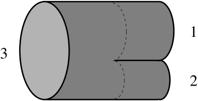
Figure 1: The three-string interaction vertex. In order to make the picture clear we have drawn a finite time interval enclosing the interaction, which occurs at the single precise moment of time. Our goal in this lecture is to write down the Feynman rule $|V\rangle$ for this simple interaction.

Our convention about the selection of $p_{3}^{+}$ guarantees that string 3 is always the ‘long string’. The interaction (61) mediates the string splitting $3\to 1+2$, or its hermitian conjugate, the joining of $1+2\to 3$. This process is depicted in Figure 1. All we have to do now is Fourier transform this delta-functional into the harmonic oscillator number basis! Let us assemble the steps of this calculation.

Step 1. First we recall the definition of a $\Delta$-functional as a product of delta-functions for each Fourier mode,

$$\Delta[x_{1}(\sigma)+x_{2}(\sigma)-x_{3}(\sigma)]=\prod_{m=-\infty}^{\infty}\delta\left(\int_{0}^{2\pi|p_{3}^{+}|}d\sigma\ e^{im\sigma/|p_{3}^{+}|}[x_{1}(\sigma)+x_{2}(\sigma)-x_{3}(\sigma)]\right).$$ (62)

Let us introduce matrices $X^{(r)}_{mn}$ which express the Fourier basis of string $r$ in terms of the Fourier basis of string 3 (so that, clearly, $X^{(3)}=1$). Then we can write

$$\Delta[x_{1}(\sigma)+x_{2}(\sigma)-x_{3}(\sigma)]=\prod_{m=-\infty}^{\infty}\delta\left(\sum_{r=1}^{3}X^{(r)}_{mn}p_{n(r)}\right).$$ (63)

These matrices are obtained by simple Fourier transforms,

$$X^{(1)}_{mn}={1\over\pi}(-1)^{m+n+1}{\sin(\pi my)\over n-my},\qquad X^{(2)}_{mn}={1\over\pi}(-1)^{n}{\sin\pi m(1-y)\over n-m(1-y)},$$ (64)

where $y=p_{1}^{+}/|p_{3}^{+}|$ is the ratio of the width of string 1 to the width of string 3.

Step 2. The expansion of the field $\Phi$ in position space is given by

$$\Phi[p^{+},x(\sigma)]={1\over\sqrt{|p^{+}|}}\sum_{\vec{N}}A_{\vec{N}}(p^{+})\prod_{n=-\infty}^{\infty}\psi_{N_{n}(x_{n})},$$ (65)

where $\psi_{N}(x)=\langle x|N\rangle$ is a harmonic oscillator wavefunction for the $N$-th excited level. When we plug (65) into the cubic action (61), we find that the coupling between the three strings labeled by $\vec{N}_{(1)}$, $\vec{N}_{(2)}$ and $\vec{N}_{(3)}$ is simply

$$c(\vec{N}_{(1)},\vec{N}_{(2)},\vec{N}_{(3)})=\int\prod_{n=-\infty}^{\infty}\psi_{N_{(1)n}}(x_{n(1)})\psi_{N_{(2)n}}(x_{n(2)})\psi_{N_{(3)n}}(x_{n(3)})dM$$ (66)

where the measure is

$$dM=fDx_{1}(\sigma)Dx_{2}(\sigma)Dx_{3}(\sigma)\Delta[x_{1}(\sigma)+x_{2}(\sigma)-x_{3}(\sigma)].$$ (67)

Step 3. The next step is to note that an $x$-eigenstate of an oscillator with frequency $\omega$ may be represented as

$$|x\rangle=({\rm constant})\exp\left[-{\omega x^{2}\over 4}+i\sqrt{2\omega}a^{\dagger}-{1\over 2}a^{\dagger}a^{\dagger}\right]|0\rangle.$$ (68)

It follows from this that

$$\sum_{N=0}^{\infty}|N\rangle\psi_{N}(x)=({\rm constant})\exp\left[-{\omega x^{2}\over 4}+i\sqrt{2\omega}a^{\dagger}-{1\over 2}a^{\dagger}a^{\dagger}\right]|0\rangle.$$ (69)

Note that the overall constant is irrelevant since we can absorb it into $f$.

Step 4. Now let us assemble the couplings $c$ into the state $|V\rangle$:

$$|V\rangle=\sum_{\vec{N}_{1},\vec{N}_{2},\vec{N}_{3}}=c(\vec{N}_{(1)},\vec{N}_{(2)},\vec{N}_{(3)})|\vec{N}_{(1)}\rangle|\vec{N}_{(2)}\rangle|\vec{N}_{(3)}\rangle.$$ (70)

Using (66) and (69), we arrive finally at

$$|V\rangle=\int dM\exp\left[\sum_{k=-\infty}^{\infty}\sum_{r=1}^{3}\left(-{\omega_{k(r)}^{2}\over 4}x_{k(r)}^{2}-{1\over 2}(a_{k(r)}^{\dagger})^{2}+i\sqrt{2\omega_{k(r)}}x_{k(r)}a_{k(r)}^{\dagger}\right)\right]|0\rangle.$$ (71)

The functional measure is just a product over all Fourier modes:

$$dM=\prod_{m=-\infty}^{\infty}\left(\sum_{r=1}^{3}\sum_{n=-\infty}^{\infty}X^{(r)}_{mn}x_{n(r)}\right)\prod_{r=1}^{3}\prod_{k=-\infty}^{\infty}dx_{k(r)}.$$ (72)

The delta-functions allow us to replace all of the modes of string 3 in terms of the modes of strings 1 and 2. Then (71) is just a Gaussian integral in the infinitely many variables $x_{k(1)}$, $x_{k(2)}$, $k=-\infty,\ldots,+\infty$!

Step 5. The Gaussian integral is easily done, and we find

$$|V\rangle=f(p_{1}^{+},p_{2}^{+},p_{3}^{+})(\det\Gamma)^{-1/2}\exp\left[{1\over 2}\sum_{r,s=1}^{3}\sum_{m,n=-\infty}^{\infty}a_{m(r)}^{\dagger}\overline{N}^{(rs)}_{mn}a_{n(s)}^{\dagger}\right]|0_{(1)}\rangle|0_{(2)}\rangle|0_{(3)}\rangle,$$ (73)

where we have absorbed a constant into $f$ (it was undetermined anyway), and we have introduced the matrices

$$\Gamma_{mn}=\sum_{r=1}^{3}\sum_{p=-\infty}^{\infty}\omega_{p(r)}X_{mp}^{(r)}X_{np}^{(r)},$$ (74)

and

$$\overline{N}^{(rs)}_{mn}=\delta^{rs}\delta_{mn}-2\sqrt{\omega_{m(r)}\omega_{n(s)}}(X^{(r){\rm T}}\Gamma^{-1}X^{(s)})_{mn}.$$ (75)

3.5 Alternate, Simpler Derivation

We now give a more straightforward way to arrive at the same final result (73). After Fourier transforming, the delta-functional can be expressed as local conservation of momentum density on the worldsheet:

$$\Delta[p_{1}(\sigma)+p_{2}(\sigma)+p_{3}(\sigma)].$$ (76)

We are trying to find a state $|V\rangle$ which is an oscillator representation of the position- and momentum-space delta-functionals. Now recall the elementary identity

$$x\delta(x)=0.$$ (77)

The state $|V\rangle$ must therefore satisfy

$$\left(p_{1}(\sigma)+p_{2}(\sigma)+p_{3}(\sigma)\right)|V\rangle=(x_{1}(\sigma)+x_{2}(\sigma)-x_{3}(\sigma))|V\rangle=0.$$ (78)

Let us take the Fourier transform of these equations with respect to the $m$-th Fourier mode of string 3. Then we make use of the same matrices $X^{(r)}$ introduced above, and we find the following equations, which must vanish for each $m$:

$$\sum_{r=1}^{3}\sum_{n=-\infty}^{\infty}X^{(r)}_{mn}p_{n(r)}|V\rangle=0,\qquad\sum_{r=1}^{3}\sum_{n=-\infty}^{\infty}e(p^{+}_{r})X^{(r)}_{mn}x_{n(r)}|V\rangle=0.$$ (79)

If we make an ansatz for $|V\rangle$ of the form

$$|V\rangle=f(p_{1}^{+},p_{2}^{+},p_{3}^{+})\exp\left[{1\over 2}\sum_{r,s=1}^{3}\sum_{m,n=-\infty}^{\infty}a_{m(r)}^{\dagger}\overline{N}^{(rs)}_{mn}a_{n(s)}^{\dagger}\right]|0_{(1)}\rangle|0_{(2)}\rangle|0_{(3)}\rangle,$$ (80)

for some coefficients $\overline{N}$, and then expand the $x$’s and $p$’s appearing in (79) into creation and annihilation operators, then one obtains some matrix equations whose unique solution is

$$\overline{N}^{(rs)}_{mn}=\delta^{rs}\delta_{mn}-2\sqrt{\omega_{m(r)}\omega_{n(s)}}(X^{(r){\rm T}}\Gamma^{-1}X^{(s)})_{mn}.$$ (81)

It is clear that $f(p_{1}^{+},p_{2}^{+},p_{3}^{+})$ remains undetermined by this method.

3.6 Summary

We have written the Hamiltonian of string theory in light cone gauge as a free term plus a cubic interaction. It turns out (at least for the bosonic string) that this is the whole story! One can use this simple Hamiltonian to calculate the string S-matrix, to arbitrary order in string perturbation theory, with no conceptual difficulties. (The remaining measure factor $f$ will be determined in the next lecture.) Since this is a light-cone gauge quantization, the procedure is especially simple. There are no ‘vacuum’ diagrams, so one just uses the simple Feynman diagrammatic expansion of the S-matrix: the only interaction vertex is a simple string splitting or joining.

4 Lecture 3: Light-Cone String Field Theory

4.1 Comments on the Neumann Coefficients

In the last lecture we wrote the cubic string vertex as a squeezed state in the three-string Fock space:

$$|V\rangle=\delta(p_{1}^{+}+p_{2}^{+}+p_{3}^{+})f(p_{1}^{+},p_{2}^{+},p_{3}^{+},\mu)(\det\Gamma)^{(2-D)/2}\exp\left[V(a_{(1)}^{\dagger},a_{(2)}^{\dagger},a_{(3)}^{\dagger})\right]|0_{(1)}\rangle|0_{(2)}\rangle|0_{(3)}\rangle.$$ (82)

Here $f(p_{1}^{+},p_{2}^{+},p_{3}^{+},\mu)$ is a measure factor which we have not yet determined and $D$ is the dimensionality of space time. This enters the formula because one gets one factor of $(\det\Gamma)^{-1/2}$ for each dimension transverse to the light cone. Finally we have made the convenient definition

$$V(a_{1},a_{2},a_{3})={1\over 2}\sum_{r,s=1}^{3}\sum_{m,n=-\infty}^{\infty}\overline{N}^{(rs)}_{mn}a_{m(r)}a_{n(s)}.$$ (83)

The matrix element $\overline{N}^{(rs)}_{mn}$ expresses the coupling between mode $m$ on string $r$ and mode $n$ on string $s$. These coefficients are called Neumann coefficients. Although the $X$ matrices are independent of $\mu$, the matrix $\Gamma$ depends on $\mu$ (and the three $p_{+}$’s) in a highly nontrivial way. In the $\mu\to 0$ limit, it is rather easy to show that these Neumann coefficients reduce correctly to the flat space case, where explicit formulas are known for $\overline{N}^{(rs)}_{mn}$ (see the papers reproduced in [11]).

A huge technology has been developed towards obtaining explicit formulas for $\overline{N}^{(rs)}_{mn}$ as a function of $\mu$ and $p_{+}^{r}$. This material is too technical to present in detail, so we will just summarize the current state of the art [77]. Recall that the dual BMN gauge theory is believed to be effectively perturbative in the parameter

$$\lambda^{\prime}={1\over(\mu p^{+}\alpha^{\prime})^{2}}.$$ (84)

So, in order to make contact with perturbative gauge theory calculations, we are particularly interested in studying string interactions in the large $\mu$ limit. In this limit it can be shown that

$$\overline{N}^{(13)}_{mn}={1\over 2\pi}{(-1)^{m+n+1}\sin(\pi ny)\over p^{+}_{3}\omega_{m(1)}+p^{+}_{1}\omega_{n(3)}}\sqrt{y\over\omega_{m(1)}\omega_{n(3)}}$$ (85)

$$\qquad\times\left[\sqrt{(\omega_{m(1)}+\mu p^{+}_{1}\alpha^{\prime})(\omega_{n(3)}+\mu p^{+}_{3}\alpha^{\prime})}+\sqrt{(\omega_{m(1)}-\mu p^{+}_{1}\alpha^{\prime})(\omega_{n(3)}-\mu p^{+}_{3}\alpha^{\prime})}\right]$$ (86)

$$\qquad\qquad+{\cal{O}}(e^{-2\pi\mu},e^{-2\pi\mu y},e^{-2\pi\mu(1-y)}).$$ (87)

The first term encodes all orders in a power series expansion in $\lambda^{\prime}$. Specifically,

$$\overline{N}^{(13)}_{mn}=\left[{(-1)^{m+n+1}\over\pi\sqrt{y}}{\sin(\pi ny)\over n-m/y}+{\cal{O}}(\lambda^{\prime})+\cdots\right]+{\mbox{nonperturbative}}.$$ (88)

It is intriguing that the nonperturbative corrections look like D-branes rather than instantons (i.e. they are ${\cal{O}}(e^{-1/g})$ rather than ${\cal{O}}(e^{-1/g^{2}})$).

We have only written the Neumann coefficient $\overline{N}^{(13)}$, but in fact it is easily shown that in the $\mu\to\infty$ limit,

$$\overline{N}^{(13)}_{mn}=\sqrt{y}X^{(1){\rm T}}_{mn},\qquad\overline{N}^{(23)}_{mn}=\sqrt{1-y}X^{(2){\rm T}}_{mn},$$ (89)

while all other components are zero. This fact actually has a very nice interpretation in the BMN gauge theory, which we present in Table 3.

‘three-point’ functions		$\longleftrightarrow$		matrix elements of $|V\rangle$
at $\lambda^{\prime}=0$				at $\mu=\infty$
	$\nwarrow\searrow$		$\nearrow\swarrow$
		matrix elements of $\Sigma$,
		splitting-joining operator

Table 3: Correspondence between the $\mu=\infty$ limit of the three-string vertex, the BMN limit of the gauge theory, and the splitting-joining operator $\Sigma$ in the string bit model [67]. This correspondence has been explored in a number of papers, including [47, 46, 71, 83].

4.2 The Consequence of Lorentz Invariance

Our vertex (82) still has an arbitrary function $f$ of the light-cone momenta and $\mu$, and a factor $(\det\Gamma)^{(2-D)/2}$, which is also a terribly complicated function of the light-cone momenta and $\mu$. In flat space ($\mu=0$), it was shown long ago that Lorentz-invariance of the vertex, and in particular, the covariance of S-matrix elements under $J^{+-}$ Lorentz transformations, requires $D=26$ and $f=(\det\Gamma)^{12}$.

This fact is nice for the oscillator representation since these factors then cancel and (82) can simply be written as

$$|V\rangle=\delta(p_{1}^{+}+p_{2}^{+}+p_{3}^{+})\exp\left[V(a_{(1)}^{\dagger},a_{(2)}^{\dagger},a_{(3)}^{\dagger})\right]|0_{(1)}\rangle|0_{(2)}\rangle|0_{(3)}\rangle,\qquad{\rm for~{}}\mu=0,$$ (90)

with no additional factors (except perhaps some innocent overall factors like $2\pi$’s which we have not carefully kept track of).

However, in the functional representation this fact is quite mysterious! It means that the correct, Lorentz-invariant string vertex in flat space,

$$H_{3}=g_{2}\int\delta(p_{1}^{+}+p_{2}^{+}+p_{3}^{+})(\det\Gamma)^{12}\Delta[x_{1}(\sigma)+x_{2}(\sigma)-x_{3}(\sigma)]\prod_{r=1}^{3}\left(dp_{r}^{+}Dx_{r}(\sigma)\ \Phi[p_{r}^{+},x_{r}(\sigma)]\right),$$ (91)

has a very peculiar measure factor $(\det\Gamma)^{12}$ which would have been impossible to guess purely within the functional approach. Moreover, since the function $(\det\Gamma)^{12}$ is a highly complicated function of the $p_{i}^{+}$, if we Fourier transform the action (91) back to $x^{-}$ position space, we find that it involves infinitely many $\partial_{x^{-}}$ derivatives, in a very complicated way. This tells us that light-cone string field theory is highly non-local in the $x^{-}$ direction.

The plane wave background with $\mu>0$ has fewer bosonic symmetries than flat space. In particular, it does not have the $J^{+-}$ or $J^{-I}$ symmetries. This means that it is impossible to use Mandelstam’s method to determine what the corresponding measure factor is when $\mu>0$. Our vertex for string interactions in the plane wave background remains ambiguous up to an overall (possibly very complicated) function of $p_{1}^{+},p_{2}^{+},p_{3}^{+}$ and $\mu$.

We determined the form of the vertex by requiring continuity of the string worldsheet, but evidently that is not enough to solve our problem. In the rest of this lecture we will learn why light-cone string field theory works, and what the physics is that does completely determine the light-cone vertex (since continuity is not enough). To be precise, we should say that we will discuss the physics which in principle determines the light-cone vertex uniquely. The actual calculation of what this overall function is has not yet been performed for $\mu>0$, and is likely rather difficult. (In the supersymmetric theory, it has been speculated that supersymmetry might fix this overall function essentially to 1, but this has not been proven.)

The first step on this exciting journey into the details of string field theory will be a close look at the four-string scattering amplitude.

4.3 A Four-String Amplitude

We consider a $2\to 2$ string scattering process at tree level. This exercise will be useful for showing how to use the formalism of light-cone string field theory to do actual calculations. Without loss of generality we can choose to label the particles so that 1 and 2 are incoming (positive $p^{+}$) and 3 and 4 are outgoing (negative $p^{+}$) and furthermore $-p_{4}^{+}>p_{1}^{+}>p_{2}^{+}>-p_{3}^{+}$.

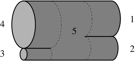
Figure 2: The $s$-channel contribution to the tree level 4-particle interaction $1+2\to 5\to 3+4$.

The $s$-channel amplitude (see Figure 2) is

$${\cal{A}}_{s}=\int_{0}^{\infty}dT_{5}\int_{0}^{p^{+}_{5}}{d\sigma_{5}\over p^{+}_{5}}\underbrace{\langle 0_{(5)}|{V(a_{4},a_{3}^{\dagger},a_{4}^{\dagger})}|0_{(3)}\rangle|0_{(4)}\rangle}_{5\to 3+4}$$ (92)

$$\qquad\qquad\qquad\times{e^{-T_{5}(E_{1}+E_{2}-H_{(5)})+2\pi i\sigma_{5}(N_{(5)}-\widetilde{N}_{(5)})/p^{+}_{5}}}\underbrace{\langle 0_{(1)}|\langle 0_{(2)}|{V(a_{1},a_{2},a_{5}^{\dagger})}|0_{(5)}\rangle}_{1+2\to 5}.$$ (93)

Let us explain each ingredient. First of all, trivial overall $p^{+}$-momentum conserving delta functions are always understood but have not been written in order to save space. The processes $1\to 2+5$ and $5\to 3+4$ are as indicated, making use of our vertex function $V$. In between these two we have inserted the light-cone propagator for the intermediate string 5:

$${1\over E-H}=\int_{0}^{\infty}dTe^{-T(E-H)}.$$ (94)

By $H_{(5)}$ we mean of course the Hamiltonian for string 5:

$$H_{(5)}={1\over p^{+}_{(5)}}\sum_{n=-\infty}^{\infty}\omega_{n(5)}a_{n(5)}^{\dagger}a_{n(5)}.$$ (95)

Finally, the integral over $\sigma_{5}$ enforces the physical state condition on the intermediate string by projecting onto those states which satisfy

$$N_{(5)}-\widetilde{N}_{(5)}=\sum_{n=-\infty}^{\infty}na_{n(5)}^{\dagger}a_{n(5)}=0.$$ (96)

The full amplitude has two additional contributions. In the $t$-channel, we have first $1\to 3+6$, and then $6+2\to 4$:

$${\cal{A}}_{t}=\int_{-\infty}^{0}dT_{6}\int_{0}^{p^{+}_{6}}{d\sigma_{6}\over p^{+}_{6}}\langle 0_{2,6}|{V(a_{2},a_{6},a_{4}^{\dagger})}|0_{4}\rangle$$ (97)

$$\qquad\qquad\qquad\times e^{-T_{6}(E_{1}-E_{3}-H_{(6)})+2\pi i\sigma_{6}(N_{(6)}-\widetilde{N}_{(6)})/p^{+}_{6}}\langle 0_{1}|{V(a_{1},a_{3}^{\dagger},a_{6}^{\dagger})}|0_{3,6}\rangle.$$ (98)

Finally in the $u$-channel, $2\to 3+7$ and then $7+1\to 4$:

$${\cal{A}}_{u}=\int_{-\infty}^{0}dT_{7}\int_{0}^{p^{+}_{7}}{d\sigma_{7}\over p^{+}_{7}}\langle 0_{1,7}|{V(a_{1},a_{7},a_{4}^{\dagger})}|0_{4}\rangle$$ (99)

$$\qquad\qquad\qquad\times e^{-T_{7}(E_{2}-E_{3}-H_{(7)})+2\pi i\sigma_{7}(N_{(7)}-\widetilde{N}_{(7)})/p^{+}_{7}}\langle 0_{2}|{V(a_{2},a_{3}^{\dagger},a_{7}^{\dagger})}|0_{3,7}\rangle.$$ (100)

What are these things? Well, each ${\cal{A}}$ is just a state in ${\cal{F}}^{4}$, the fourth power of the string Fock space. If we want to know the amplitude for scattering four particular external states, then we just have to calculate

$$\langle 3|\langle 4|{\cal{A}}|1\rangle|2\rangle$$ (101)

(summed over channels) to get the scattering amplitude as a function of $p^{+}_{i}$ and $\mu$.

It should be emphasized that the harmonic oscillator algebra gives very complicated functions of $T$ and $\sigma$ which need to be integrated over. Actually performing this calculation is far outside the scope of these lectures (see [4]), but we would like to make one very important point about the general structure of this amplitude.

Let us denote ${\cal{R}}_{i}=\{(T_{i},\sigma_{i}):T\in[0,\infty),\sigma_{i}\in[0,p^{+}_{i}]\}$, which are the two dimensional regions over which the quantities ${\cal{A}}_{i}$ must be integrated. There exists a particular map $z(T_{i},\sigma_{i})$ which patches together these three coordinate regions onto a sphere as shown in Figure 3. This much is of course obvious.

Figure 3: A schematic picture of the moduli map for the tree level 4-particle interaction.

Let us define ${\cal{A}}(z)$ to be the image of the three individual ${\cal{A}}_{s}$, ${\cal{A}}_{t}$, and ${\cal{A}}_{u}$ on the sphere, patched together via the moduli map. It turns out that in flat space, precisely in the critical dimension $D=26$, the function ${\cal{A}}(z)$ on the sphere is continuous along the boundaries between the images of ${\cal{R}}_{i}$ (that is, continuous along the dark lines in Figure 3), which means that the amplitude can be written as

$$\sum_{i=s,t,u}\int_{{\cal{R}}_{i}}dT_{i}d\sigma_{i}{\cal{A}}_{i}=\int_{S^{2}}d^{2}z\ {\cal{A}}(z).$$ (102)

4.4 Why Light-Cone String Field Theory Works

The right hand side of (102) has a very familiar form. When we studied string theory, we learned that in order to calculate a four-string amplitude at tree level in closed string theory, one inserts four vertex operators on the sphere. The positions of three vertex operators can be fixed using the conformal Killing vectors, and one is left with some amplitude (depending on the particular vertex operators inserted) which must be integrated over $z$, the position of the remaining vertex operator. The moduli space of a sphere with four marked points (the positions of vertex operators) is therefore the sphere itself.

It turns out that the integrand ${\cal{A}}(z)$ on the right-hand side of (102) is precisely the integrand one would derive from the Polyakov path integral in the covariant formulation of string theory. Although we have studied only one of the most trivial possible amplitudes, the equation (102) indicates a very general feature. Amplitudes calculated in light-cone string field theory, with any number of external states and at arbitrary order in string perturbation theory, are precisely equivalent to those calculated using the covariant Polyakov path integral [15]. This equivalence relies on two important facts:

Property 1: Triangulation of Moduli Space. Consider all of the light-cone diagrams which contribute to an amplitude with $g$ closed string loops and $n$ external particles [13]. The diagrams will be labeled by $6g+2n-6$ parameters: $g$ ‘$p^{+}$-momentum fractions’, $3g+n-3$ twist angles (to impose the physical state condition on intermediate string states), and $2g+n-3$ interaction times. The first important fact is that the moduli map provides a one-to-one map between this $6g+2n-2$-dimensional parameter space and the moduli space of Riemann surfaces of genus $g$ with $n$ marked points (the locations of the vertex operators). A mathematical way of saying this is that the light-cone vertex provides a triangulation of the moduli space ${\cal{M}}_{g,n}$.

Property 2: The Measure on Moduli Space. The second important fact is that the integrand of the light-cone vertex, including all of the complicated structure involving the Neumann matrices and determinants thereof, maps under the moduli map to precisely the correct integration measure which arises from the Polyakov path integral!

The proof of these remarkable facts would take us too far afield, but we cannot stress enough the importance of these facts, which are deeply rooted in the underlying beautiful consistency of string theory. In fact, this equivalence can be used to prove the unitarity of the Polyakov path integral [15]: although the path integral is not manifestly unitary, it is equivalent to the light-cone formalism, which is manifestly unitary!

We are now in a position to answer some questions which may have been bothering some students since the last lecture: why is it sufficient to consider a cubic interaction between the string fields, and why is it sufficient to consider the simplest possible cubic interaction, with only a delta-functional (and, for example, no derivative terms like $\delta\Phi[x(\sigma)]/\delta x(\sigma_{\rm I})$)? The answer is that the simple cubic interaction is sufficient because (1) the iterated cubic interaction covers precisely one copy of moduli space and (2) the vertex we wrote down precisely reproduces the correct integration measure on this moduli space. We don’t need anything else!

It is sometimes said that the symmetry algebra (in particular, the supersymmetry algebra, for superstrings), uniquely determines the interacting string Hamiltonian to all orders in the string coupling. This is a little bit misleading. For example, in the supersymmetric theory one could take $Q=({\rm anything})$ and then define $H=({\rm anything})^{2}$, and as long as (anything) commutes with rotations and translations, one would have a realization of the symmetry algebra! The symmetry argument, however, provides no motivation for considering only a cubic interaction. The true criteria are (1) and (2) listed above, and fortunately it turns out to be true that (at least for the bosonic string), one can find a purely cubic action with properties (1) and (2).

4.5 Contact Terms

Now, fact number (1), that the cubic delta-functional vertex covers moduli space precisely once, is essentially a mathematical theorem about a particular cell decomposition of ${\cal{M}}_{g,n}$ that holds quite generally [13]. However, (2) can fail in subtle ways in certain circumstances.

In particular, it can happen that one or more of the ${\cal{A}}_{i}$’s has singularities in moduli space. A typical case might be for example that ${\cal{A}}_{i}(T,\sigma)\sim{1\over T^{3}}$ near $T=0$, which is not integrable. This gives rise to divergences in string amplitudes, which need to be corrected by adding new string interactions to the Hamiltonian. However, these interaction terms are always delta-function supported on sets of measure zero ($T=0$ in this example) in moduli space, and therefore they do not spoil the beautiful triangulation that the cubic vertex provides. As long as we don’t add any interaction with finite measure, the triangulation still works just fine.

Definition. We define a contact term to be any term in the Hamiltonian which has support only on a set of measure zero in moduli space.

Corollary. All contact terms are divergent. Proof: If they were finite, they wouldn’t give any contribution, there would be no point to include them, since by definition they are integrated over sets of measure zero!

In flat space, it is known [15] that the bosonic string requires no contact terms, while the IIB superstring is widely (though not universally) believed to require an infinite number of contact terms. The word ‘believe’ can be thought of in the following sense: since the purpose of contact terms is to eliminate divergences (and indeed we will see how they arise from short-distance singularities on the worldsheet), one can think of a contact term as a counterterm in the sense of renormalization. Now, there are infinitely many such counter terms that one can write down for the IIB string, and while some of them may have coefficients which are equal to zero, it is widely believed that infinitely many of them will have nonzero coefficients.

For example, in open superstring field theory, it was argued in [10] that a possible contact term in the $s$-channel of the $2\to 2$ amplitude in fact vanishes. However, it was argued in [14] that there is a contact term for this process in the $u$-channel. For higher amplitudes the situation is much more complicated and has not been addressed in detail. A non-zero contact term in the one-loop mass renormalization has been studied in the plane wave background [79] and will be discussed in the next lecture.

For strings in the plane wave background, the question of whether property (2) holds has not been addressed, mostly because we do not have the analogue of the covariant Polyakov formalism in which we can actually calculate anything. First we would need to calculate this overall factor $f(p_{1}^{+},p_{2}^{+},p_{3}^{+},\mu)$ and then see if there are any divergences which give rise to contact terms.

Any of the contact terms in IIB string theory in flat space will surely give rise to $\mu$-dependent contact terms in the plane wave background. In principle there could be new contact terms introduced which go to zero in the limit $\mu\to 0$. Certainly we do not know how to disprove such a possibility, but we believe this is unlikely: contact terms may be thought of as coming from short-distance singularities on the string worldsheet, but the addition of a mass parameter $\mu$ on the worldsheet should not affect any of the short-distance behavior.

In fact, it is more likely that the opposite is true: that there are infinitely many contact terms in flat space, but all but a finite number vanish in the plane wave background when $\mu$ is large [71]. We will have more to say about this in the next lecture.

4.6 Superstrings

Let’s go back to the beginning of Lecture 2, but add fermions to the picture. We consider now a superparticle on the plane wave solution of IIB supergravity. The physical degrees of freedom of the theory are encoded in a superfield $\Phi(x,\theta)$ which has an expansion of the form [7, 30]

$$\Phi(p^{+},x,\theta)=(p^{+})^{2}A(x)+p^{+}\theta^{a}\psi_{a}(x)+\theta^{a_{1}}\theta^{a_{2}}p^{+}A_{a_{1}a_{2}}(x)+\cdots+{1\over(p^{+})^{2}}\theta^{8}A^{*}(x),$$ (103)

where $\theta$ is an eight-component SO(8) spinor ($\theta^{8}$ is short for eight powers of $\theta$ contracted with the fully antisymmetric tensor $\epsilon$). Initially we allow all the component fields to be complex, but this gives too many components (256 bosonic $+$ 256 fermionic) so we impose the reality condition

$$\Phi(x,\theta)=(p^{+})^{4}\int d^{8}\theta^{\dagger}e^{i\theta\theta^{\dagger}/p^{+}}(\Phi(x,\theta))^{\dagger}$$ (104)

which cuts the number of components in half. Note, in particular, that this constraint correctly gives the self-duality condition for the five-form field strength.

When we second quantize, this hermiticity condition implies that the inner product on the string field theory Hilbert space ${\cal{H}}$ is not the inner product naïvely inherited from the single string Hilbert space. Instead,

$${\cal{A}}_{|a\rangle}(p^{+})^{\dagger}={\cal{A}}_{|a^{\prime}\rangle}(-p^{+}),$$ (105)

where the states $|a\rangle$ and $|a^{\prime}\rangle$ differ by reversing the occupation of all of the fermionic zero modes, i.e. if $|a\rangle=|0\rangle$, then $|a^{\prime}\rangle=\theta^{8}|0\rangle$, etc.

The action for the free superparticle is

$$S={1\over 2}\int d^{10}xd^{8}\theta\ \Phi(\nabla^{2}-2i\mu\partial_{-}\theta\Pi\partial_{\theta})\Phi,$$ (106)

where $\Pi=\Gamma^{1}\Gamma^{2}\Gamma^{3}\Gamma^{4}$. The quantity in brackets is the quadratic Casimir of the plane wave superalgebra. It is straightforward to insert the superfield (104) into (106) and find the resulting spectrum [30].

The action (106) of course may also be obtained simply by linearizing the action for IIB supergravity around the plane wave background, and the spectrum may be obtained by linearizing the equations of motion around the background and finding the eigenmodes. This has been worked out in detail in [30], but we will use only one fact which emerges from this analysis. It turns out that there is a unique state with zero energy, which we will call $|0\rangle$. The corresponding spacetime field is a linear combination of the trace of the graviton over four of the eight transverse dimensions, $h_{ii}$, and the components of the four-form gauge potential $a_{1234}$ in the first four directions. This field lives in the $\theta_{\rm R}^{4}$ component of the superfield, where we define left and right chirality with respect to $\Pi$ (i.e., $\theta_{\rm R,L}={1\over 2}(1\pm\Pi)\theta$). The only important fact which you might want to keep in mind is that this spacetime field is odd under the ${\mathbb{Z}}_{2}$ symmetry which exchanges the two SO(4)’s:

$$Z{\cal{A}}_{|0\rangle}=-{\cal{A}}_{|0\rangle}Z.$$ (107)

The full string theory Hamiltonian (including interactions) commutes with the ${\mathbb{Z}}_{2}$ operator $Z$, and this fact together with (107) can be used to derive useful selection rules for string amplitudes.

When we promote the superfield to string theory, it becomes a functional of the embedding of the string into superspace: $\Phi[p^{+},x(\sigma),\theta(\sigma)]$. The cubic interaction term has a delta-functional for continuity of $x(\sigma)$, and also a delta-functional for the superspace coordinates:

$$\Delta[\theta_{1}(\sigma)+\theta_{2}(\sigma)-\theta_{3}(\sigma)].$$ (108)

One can write this delta-functional in an oscillator representation as a squeezed state involving the fermionic creation operators. The ‘fermionic’ Neumann matrices are easily obtained from the bosonic Neumann matrices.

5 Lecture 4: Loose Ends

5.1 The ‘Prefactor’

From the preceding section one might have the impression that light-cone string field theory for fermionic strings is a relatively trivial modification of the bosonic theory. Unfortunately, this is not true. In the fermionic theory the cubic string interaction is no longer a simple $\Phi^{3}$ vertex with derivatives. Instead it is quadratic in string field functional derivatives. One way to see why this is necessary is to look at the supersymmetry algebra, which constrains the form of the Hamiltonian and dynamical supercharges.

The (relevant part of the) spacetime supersymmetry algebra is

$$\{Q^{-},\overline{Q}{}^{-}\}=2H,\qquad[Q^{-},H]=0,\qquad[\overline{Q}{}^{-},H]=0.$$ (109)

At the free level, a realization of this algebra is given by the free Hamiltonian $H_{2}$ we met before, and the free supercharges $Q^{-}_{2}$, which are given by

$$Q_{2}^{-}=\int dp^{+}\ p^{+}\Phi^{\dagger}q^{-}\Phi,$$ (110)

where the worldsheet supercharge is

$$q^{-}=\int d\sigma\left[4\pi e(p^{+}_{r})p^{I}\gamma_{I}\lambda-{i\over 4\pi}\partial_{\sigma}x^{I}\gamma_{I}\theta-i\mu x^{I}\gamma\Pi\lambda\right].$$ (111)

Here $\lambda$ is the ‘fermionic momentum’ conjugate to $\theta$ (i.e., it is just $\overline{\theta})$).

When we turn on an interaction $H_{3}$ in the Hamiltonian, we also need to turn on interactions $Q_{3}$, $\overline{Q}{}_{3}$ in the dynamical supercharges to ensure that the generators

$$H=H_{2}+g_{s}H_{3},\qquad Q^{-}=Q^{-}_{2}+g_{2}Q^{-}_{3},\qquad\overline{Q}^{-}=\overline{Q}^{-}_{2}+g_{s}\overline{Q}^{-}_{3}$$ (112)

provide a (non-linear) realization of the supersymmetry algebra (109).

Now there is a simple argument (see chapter 11 of [12]) which shows that the choice $|H_{3}\rangle=|V\rangle$ would be incompatible with the supersymmetry algebra. Consider the relation $0=[\overline{Q}{}^{-},H]$ at first order in the string coupling. This gives (via the state-operator correspondence)

$$0=\sum_{r=1}^{3}H_{(r)}|Q^{-}\rangle+\sum_{r=1}^{3}Q_{(r)}^{-}|V\rangle.$$ (113)

Now let us consider (for example) a matrix element of this relation where we sandwich three on-shell states on the left. Then $\sum_{r=1}^{3}H_{(r)}$ acts to the left and gives zero, leaving us with only the second term. Now the state $|V\rangle$ indeed is annihilated by the constraints

$$\sum p_{(r)}|V\rangle=\sum\lambda_{(r)}|V\rangle=\sum e(p^{+}_{r})x_{(r)}|V\rangle=\sum e(p^{+}_{r})\theta_{(r)}|V\rangle=0.$$ (114)

Now after looking at (111), the conditions (114) seem to imply that $Q_{(r)}^{-}|V\rangle=0$, and hence that the desired relation (113) is true.

However, one can check that the operators in (111) are actually singular near the interaction point. For example, we have $p(\sigma)\lambda(\sigma)|V\rangle\sim\partial_{\sigma}x(\sigma)\theta(\sigma)|V\rangle\sim\epsilon^{-1}|V\rangle$ near $\sigma=\sigma_{\rm I}$. Therefore, although $\sum_{r=1}^{3}Q_{(r)}^{-}|V\rangle$ vanishes pointwise in $\sigma$ (except at $\sigma=\sigma_{\rm I}$), the singular operators nevertheless give a finite contribution when integrated over $\sigma$. This contribution can be calculated by deforming the $\sigma$ contour in an appropriate way and reading off the residue of the pole at $\sigma=\sigma_{\rm I}$.

By calculating the residue of this pole, it can be shown that in order to supersymmetrize the vertex, it is necessary to introduce some operators (called ‘prefactors’) $\hat{h}$, $\hat{q}{}^{-}$, $\overline{\hat{q}}{}^{-}$ such that the interacting Hamiltonian and supercharges are given by

$$|H_{3}\rangle=\hat{h}|V\rangle,\qquad|Q_{3}\rangle=\hat{q}|V\rangle,\qquad|\overline{Q}{}_{3}\rangle=\overline{\hat{q}}{}^{-}|V\rangle.$$ (115)

It turns out that $\hat{h}$ is a second-order polynomial in bosonic mode-creation operators (the $a^{\dagger}$’s) while $\hat{q}$ and $\overline{\hat{q}}{}^{-}$ are linear in bosonic creation operators. They also have a very complicated expansion in terms of fermionic modes, and we will not give the complete formula here.

It is essential to note, however, that the last term in (111) is non-singular when acting on $|V\rangle$. This makes sense, since the parameter $\mu$ introduces a scale in the worldsheet theory, but this should not affect the short distance physics. Therefore the functional form of the prefactor has essentially the same form as in flat space (there are subtleties in passing from the functional representation to the oscillator representation, though).

We have shown that in the functional representation, the cubic interaction between three string super-fields is not given simply by the delta-functionals

$$\Delta[x_{1}(\sigma)+x_{2}(\sigma)-x_{3}(\sigma)]\Delta[\theta_{1}(\sigma)+\theta_{2}(\sigma)-\theta_{3}(\sigma)]\prod_{r=1}^{3}\Phi[x_{r}(\sigma),\theta_{r}(\sigma)]$$ (116)

In addition, there is a complicated combination of functional derivatives acting on the $\Phi$ fields, inserted at the point $\sigma_{\rm I}$ where the strings split. This interaction point operator is sometimes called the ‘prefactor’. The presence of this prefactor is associated with the picture changing operator in the covariant formulation.

5.2 Contact Terms from the Interaction Point Operator

The prefactor $\hat{h}$ is an operator of weight ${3\over 2}$, which means that at short distances we have $\hat{h}(x)\hat{h}(y)\sim(x-y)^{-3}$. (In light-cone gauge we don’t have a conformal field theory in the pp-wave, so by ‘weight’ we simply mean the strength of the coincident singularity.) A light-cone string diagram in which two (or more) of these prefactors come very close to each other will therefore be divergent. The simplest example occurs in the two-particle amplitude at one loop (i.e., a contribution to the one-loop mass renormalization), shown in Figure 4. This amplitude has been studied in the $\mu\to\infty$ limit of the plane wave background in [79].

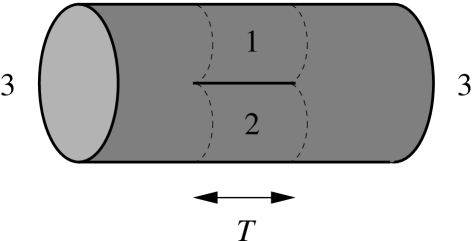
Figure 4: The one-loop mass renormalization of string 3.

This amplitude has an integral $\int_{0}^{\infty}dT$ over the Schwinger parameter giving the light-cone time between the splitting and joining (think of it as coming from the propagator (94) for the intermediate state), but the integrand is divergent like $T^{-3}$ due to the colliding prefactors. It is clear that at higher order in the string coupling (and/or with more external states), we can draw diagrams which have arbitrarily many colliding prefactors. These divergent contributions to string amplitudes must be rendered finite by the introduction of (divergent) contact interactions as discussed in the previous lecture. The belief is that there is a unique set of contact interactions which preserves all the symmetries (Lorentz invariance, supersymmetry) and which renders all amplitudes finite. But these contact terms are very unwieldy, and almost impossible to calculate explicitly, so they haven’t really been studied in very much detail.

We will have a little bit more to say about these contact terms below.

5.3 The $S$-matrix in the BMN Correspondence

In past couple of lectures we have demonstrated how to determine the light-cone Hamiltonian of second-quantized IIB string theory in the plane wave background. The two remaining ambiguities are (1) that we have not determined some overall factor $f(p_{1}^{+},p_{2}^{+},p_{3}^{+},\mu)$ that appears in the cubic coupling, and (2) that there are (probably) infinitely many contact counterterms which need to be added to the action. In principle (although probably not in practice), the light-cone string field theory approach allows one to calculate $S$-matrix elements to arbitrary order in the string coupling via a quite straightforward Hamiltonian approach: there is a (large) Hilbert space of states, with a light-cone Hamiltonian acting on it, and one can easily apply the rules of quantum mechanical perturbation theory to give the $S$-matrix

$$\langle 1|S|2\rangle=\langle 1|1-2\pi i\delta(E_{1}-E_{2})T(E+i\epsilon)|2\rangle,$$ (117)

where $H_{2}|E_{i}\rangle=E_{i}$ and $T(z)$ is the transition operator

$$T(z)=V+VG(z)V,\qquad V\equiv H-H_{2},\qquad G(z)=(z-H)^{-1}$$ (118)

which is usually calculated via the Born series

$$T(z)=V+VG_{0}(z)V+VG_{0}(z)VG_{0}(z)V+\cdots,$$ (119)

where $G_{0}(z)=(z-H_{2})^{-1}$ is the ‘bare’ propagator.

Typically, the $S$-matrix is the only good ‘observable’ of string theory. Local observables are not allowed because string theory is a theory of quantum gravity, and in particular has diffeomorphism invariance. The question is then, how is the string $S$-matrix encoded in the BMN limit of ${\cal{N}}=4$ Yang-Mills theory? Note that we are not talking about the $S$-matrix of the gauge theory (which doesn’t exist, since it is a conformal field theory). Instead, the question is about how the string theory $S$-matrix can be extracted from the BMN limit of the gauge theory.

5.4 The Quantum Mechanics of BMN Operators

It has been emphasized by a number of authors that it can be useful to think of gauge theory in the BMN limit as a quantum mechanical system [62, 67, 82]. There is a space of states (the BMN operators), an inner product (the free gauge theory two-point function), and a Hamiltonian, given by $\Delta-J$. Perturbation theory in the gauge theory organizes itself into the two parameters

$$\lambda^{\prime}={\lambda\over J^{2}}={g_{\rm YM}^{2}N\over J^{2}},\qquad g_{2}={J^{2}\over N},$$ (120)

which are respectively the effective ’t Hooft coupling and the effective genus counting parameter, respectively.

Recall that the spectrum of BMN operators takes the following form

$$\Delta-J=\sum_{n=-\infty}^{\infty}N_{n}\sqrt{1+\lambda^{\prime}n^{2}},$$ (121)

where $N_{n}$ is the number of impurities with phase $n$. To one-loop, the gauge theory Hamiltonian $H=\Delta-J$ takes the following form [82]

$$H=\underbrace{\sum_{n=-\infty}^{\infty}N_{n}+\lambda^{\prime}\sum_{n=-\infty}^{\infty}{1\over 2}n^{2}N_{n}}_{H_{0}}+\underbrace{\lambda^{\prime}g_{2}(H_{+}+H_{-})}_{V},$$ (122)

where $H_{+}$ and $H_{-}$ respectively increase and decrease the number of traces. That is, if we act with $H_{+}$ on a $k$-trace operator, then it ‘splits’ one of the traces so that we get a $k+1$-trace operator. Similarly $H_{-}$ ‘joins’ two traces.

The first two terms in (122) are clearly just the first two terms in (121), expanded to order $\lambda^{\prime}$, so we have labeled them $H_{0}$ — they constitute the ‘free’ Hamiltonian. The third term in (122) has the structure of a three-string vertex, and incorporates the string interactions, so we have labeled this term $V$.

The next step is to recall that we should keep in mind the basis transformation that appeared in the lectures of H. Verlinde in this school. In our first lecture we identified a precise correspondence between single-trace operators in the gauge theory and states in string theory. It is natural therefore to identify a double-trace operator in the gauge theory with the corresponding two-particle state in the string theory, etc. However this identification breaks down at $g_{2}\neq 0$. One way to see this is to note that in string theory, a $k$ particle state and an $l$ particle state are necessarily orthogonal (by construction) for $k\neq l$. However in the gauge theory, it is not hard to check that the gauge theory overlap (given by the two-point function in the free theory) is typically given by

$$\langle O_{\rm k-trace}(x)O_{\rm l-trace}(0)\rangle\sim g_{2}^{|k-l|}.$$ (123)

It has been conjectured [67] that one can write an exact formula, valid to all orders in $g_{2}$, for the inner product:

$$\langle 1|2\rangle=\left(e^{g_{2}\Sigma}\right)_{12},$$ (124)

where $\Sigma$ is the simple ‘splitting-joining’ operator of the bit model (see Table 3). The inner product (124) is diagonalized by the basis transformation $S^{1/2}=e^{g_{2}\Sigma/2}$. Therefore, we propose the following BMN identification at finite $g_{2}$ [71]:

$$|0;p^{+}\rangle \Longleftrightarrow S^{-1/2}{\rm Tr}[Z^{J}],$$ (125)

$$(a^{i}_{0})^{\dagger}|0;p^{+}\rangle \Longleftrightarrow S^{-1/2}{\rm Tr}[\phi^{i}Z^{J}],$$ (126)

$$(a^{i}_{n}a^{j}_{-n})^{\dagger}|0;p^{+}\rangle \Longleftrightarrow S^{-1/2}\sum_{k=0}^{J}e^{2\pi ikn/J}{\rm Tr}[\phi^{i}Z^{k}\phi^{j}Z^{J-k}],$$ (127)

$${\mbox{e}tc.}$$ (128)

Now the multi-particle states constructed from the operators on the right hand side of this correspondence will have the property that $k$-string states are orthogonal to $l$-string states for $k\neq l$. However, we have lost the identification of ‘number of traces’ with ‘number of strings’. Instead, we have something of the form

$${\mbox{$k$-string state}}\Longleftrightarrow[{\mbox{$k$-trace operator}}]$$ (129)

$$\qquad\qquad+g_{2}\times[{\mbox{$k{-}1$-trace operator}}+{\mbox{$k{+}1$-trace operator}}]+\cdots$$ (130)

It is convenient to perform this basis transformation on the operator $H$, to define what we will call the string Hamiltonian $\widetilde{H}$, given by

$$\widetilde{H}=S^{1/2}HS^{-1/2}\equiv H_{0}+W,$$ (131)

for some new interaction $W$ (which is easily calculated). Now $\widetilde{H}$ is simply a non-relativistic quantum mechanical Hamiltonian, and it is straightforward to derive from it an $S$-matrix. This $S$-matrix should be that of IIB string theory on the plane wave background. It is important to recognize that this $S$-matrix is not unitarily equivalent to the $S$-matrix obtained from the Hamiltonian $H_{0}+V$ [89].

5.5 Contact Terms from Gauge Theory

Previously we compared contact terms to counterterms, and we saw how certain contact terms in the superstring come about from regulating singularities that arise when two operators collide on the worldsheet. One could imagine regulating the theory in some way in order to render these divergences finite. One natural regulator, which is suggested by both the dual gauge theory and the string bit model, is to discretize the worldsheet.

Discretizing the worldsheet leads to a spacetime Hamiltonian which depends on $J$, the total number of bits. Schematically, we might have something like

$$H(J)=H_{2}(J)+H_{3}(J)+\sum_{k=1}^{\infty}J^{k}C_{k}(J),$$ (132)

where we suppose that $C_{k}(J)$ are finite in the $J\to\infty$ limit. When $J$ is finite, the cubic interaction $H_{3}(J)$ will fail to precisely cover the moduli space, but the additional ‘contact terms’ will be finite and will cover regions of moduli space of small but nonzero measure. In the continuum limit $J\to\infty$, the contact terms become infinite but restricted to regions of measure zero.

Physical quantities (such as $S$-matrix elements) should of course be independent of the regulator $J$. The precise way to say this is that the amplitudes obtained from $H(J_{1})$ differ from those obtained from $H(J_{2})$, $J_{1}\neq J_{2}$ by something which is BRST-exact. Anything BRST-exact integrates to zero over moduli space, so this is a sufficient condition for amplitudes to indeed be independent of the cutoff $J$.

The previous two paragraphs have been well-motivated, but not precise: in fact, we do not know how to make precise sense of $H(J)$ in string theory. Certainly discretized string theories have been considered in the past (see for example [5, 6, 19]), but including interactions is frequently problematic. The bit model [48, 67] is intended as a step in the direction of constructing $H(J)$.

Perhaps, however, the best way to make $H(J)$ precise is simply to read it off from the gauge theory! Comparing matrix elements of $\Delta-J$ in the gauge theory to matrix elements of (132) would let us read off the contact terms perturbatively in the $\lambda^{\prime}\sim 1/\mu^{2}$ expansion.

6 Summary

In these lectures we have learned that the essence of light-cone string field theory is an interacting string Hamiltonian which satisfies Properties 1 and 2 from Lecture 3. Furthermore, we learned how to construct a Hamiltonian which satsfies these properties, except possibly for measure zero contact interactions for the superstring. We also learned a little bit about the BMN limit of the ${\cal{N}}=4$ SU($N$) Yang-Mills theory. An obvious goal, which has been realized in a number of papers, is to check whether the BMN limit of the gauge theory can reproduce string amplitudes in the plane wave background. We now summarize the successses of this research program, and end the lectures with a list of open questions.

6.1 String Interactions in the BMN Correspondence

Following closely the original construction of [9] in flat space, the three-string vertex for type IIB superstring field theory in the plane-wave background has been constructed [39, 50, 73], including the bosonic and fermionic Neumann coefficients, matrix elements of the prefactor, and even explicit formulas for the Neumann coefficients to all orders in $\lambda^{\prime}$ [77]. Matrix elements of the cubic interaction in string field theory have been successfully matched to matrix elements of $\Delta-J$ in the dual gauge theory after taking into account the relevant basis transformation discussed above [62, 71, 72, 79]. This program is highly developed and further aspects of this approach have been studied in [43, 45, 46, 49, 53, 54, 56, 60, 61, 64, 65, 70, 78, 80, 84, 86, 89, 91, 94, 99, 101, 103, 104, 107].

All of the successful checks of this correspondence have been restricted to amplitudes where the number of impurities (in the gauge theory language) is conserved. For such amplitudes, all calculations so far indicate that the gauge theory can indeed match the string theory prediction, even though we are in a large ’t Hooft coupling limit of the gauge theory. The successful match works quite generally at first order in $\lambda^{\prime}$ and $g_{2}$, and at order $g_{2}^{2}$ (when intermediate impurity number violating processes are omitted). Although there is no obstacle in principle to pushing these checks to higher order, the light-cone string field theory becomes prohibitively complicated.

Since it is obvious that the repeated splitting and joining (i.e., $k$-trace operators to $k{\pm}1$-trace operators) in the gauge theory provides, in the large $J$ limit, a triangulation of the string theory moduli space (Property 1), these successful tests of the BMN correspondence amount to checking that the gauge theory also knows about the correct measure on moduli space (Property 2), at least in some limits of $\lambda^{\prime}$ and $g_{2}$ parameter space.

6.2 Some Open Questions and Puzzles

We conclude our lectures with a partial list of open problems and interesting directions for further research.

Explore the Structure of the String Field Theory. Can we say more about light-cone string field theory in the plane wave background? In particular, is it possible to determine the measure factor $f(p_{1}^{+},p_{2}^{+},p_{3}^{+},\mu)$? Is it possible to fully calculate a 4-particle interaction, or a 1-loop mass renormalization? What can be said about the contact terms in the large $\mu$ limit?

Does an $S$-matrix Exist in the Plane Wave? See references [69, 75, 95, 109, 92]. Obviously, we have assumed in these lectures that the answer is yes. The existence of an $S$-matrix has several very interesting consequences which should be possible to check purely within the gauge theory. For example, it implies that the one-loop mass renormalization of any $k$-particle state should be equal to the sum of the one-loop mass renormalizations of the individual particles. This is because the existence of an $S$-matrix presupposes that the particles can be well-separated from each other (in the $x^{-}$ direction). For the most trivial case, where one particle has 2 impurities, and the other $k{-}1$ particles are all in the ground state, ${\rm Tr}[Z^{J}]$, this has indeed been shown to be true (it is essentially due to the fact that ‘disconnected’ diagrams dominate over ‘connected’ ones in the large $J$ limit—see [80] for details). Can this proof be generalized to $k$ operators, each of which has more than zero (ideally, arbitrarily many) impurities?

Calculate the Gauge Theory Inner Product. The gauge theory inner product is defined as the coefficient of the free ($g_{\rm YM}=0$) two-point function. For example, in the simplest case of two vacuum operators it has been shown that [40, 43]

$$\langle{\rm Tr}[\overline{Z}^{J}]{\rm Tr}[Z^{J}]\rangle={\sinh(g_{2}/2)\over g_{2}/2}.$$ (133)

For BMN operators with impurities, the inner product has been calculated only to a couple of orders in $g_{2}$. Since this is a free gauge theory calculation, it reduces to a simple Gaussian matrix model, with graphs of genus $g$ contributing at order $g_{2}^{2g}$. It should be possible to prove (or disprove!) the conjectured formula that the inner product is given in general by $e^{g_{2}\Sigma}$, where $\Sigma$ is the splitting-joining operator of the bit model.

‘Solve’ the Quantum Mechanics of BMN Operators. Recent studies have uncovered hints of integrable structures in ${\cal{N}}=4$ gauge theory. One interesting question is whether there is any more hidden structure in the quantum mechanical Hamiltonian we wrote down. For example, one can check (at least in the two-impurity sector) that the interaction $W$ in the string Hamiltonian ${\widetilde{H}}$ commutes with $\Sigma$ [89]! Are there any other hidden symmetries which will allow one to make progress towards solving this quantum mechanics?

Do Higher-Point Functions Play any Role in the BMN Limit? In our discussion we limited our interest purely to two-point functions in the gauge theory (although we did consider two-point functions of $k$-trace operators with $l$-trace operators, but that contains only a tiny remnant of the information encoded in the $k+l$-point function). These two-point functions were interpreted (essentially) as $S$-matrix elements. It is natural to wonder (as many papers have) what (if any) role is played by the higher-point functions.

In the previous lecture we explained the correspondence between three-point functions, matrix elements of $|V\rangle$, and matrix elements of $\Sigma$ at $\lambda^{\prime}=0$. We avoided attempting to extend this correspondence to $\lambda^{\prime}>0$ for the following reason. In a conformal field theory, three-point functions of operators with well-defined scaling dimension have simple three-point functions. But BMN operators do not have well-defined scaling dimension when $g_{2}>0$! They are eigenstates of the ‘free’ Hamiltonian $H_{0}$, but they are not eigenstates of $H=\Delta-J$. So in general, the three-point function of BMN operators looks like

$$\langle O_{1}(x_{1})O_{2}(x_{2})O_{3}(x_{3})\rangle={\mbox{very complicated function of }}(x_{1},x_{2},x_{3}).$$ (134)

We do not know how to recover the $x_{1}$, $x_{2}$, $x_{3}$ dependence of (134) from the string theory side.

Another point to keep in mind is that higher-point functions of BMN operators typically diverge in the large $J$ limit [40]. An interesting alternative is to consider $n$-point functions where 2 operators are BMN, and $n{-}2$ operators have finite charge (for example, ${\rm Tr}[\phi Z]$). Such an $n$-point function might be interpreted as an amplitude for propagation from some initial state to some final state, with $n{-}2$ other operators inserted on the worldsheet which perturb the spacetime away from the pure pp-wave background. The correspondence between spacetime perturbations and operator insertions can be read off from the familiar dictionary of $AdS_{5}\times S^{5}$. Some calculations along these lines have been performed in [97, 98].

Define $H(J)$ Precisely and Provide a String Theory Construction for It. Equivalently, Can Continuum Light-Cone Superstring Field Theory be Honestly Discretized? Discretized string theories have been studied for a long time (in particular by Thorn [5, 6, 19]), but it seems somewhat problematic to discretize an interacting type IIB string. In particular, there are problems with the fermions. There is the usual fermion doubling problem (see [85, 100, 106]) that was mentioned briefly in the lectures of H. Verlinde. There is also the basic question of how to implement the hermiticity constraint (105), which in the continuum theory singles out the fermionic zero modes from the non-zero modes. However, a discretized string doesn’t really have any fermionic zero modes, there is just one fermionic oscillator on each ‘site’ along the string, and the natural ‘adjoint’ just takes the adjoint of each fermion at each site, in contrast with (105).

Which Quantities can be Calculated Perturbatively in the Gauge Theory? It is important to not forget that the BMN limit still involves taking the ’t Hooft coupling to infinity, so the weak coupling expansion is not really valid. However, it is empirically observed that some quantities, notably the conformal dimensions of BMN operators at $g_{2}=0$:

$$\Delta-J=\sum_{n=-\infty}^{\infty}N_{n}\sqrt{1+\lambda^{\prime}J^{2}},$$ (135)

may be calculated at small $\lambda$ (i.e., in gauge theory perturbation theory) and finite $J$, and then extrapolated to $\lambda,J\to\infty$ where magically they agree with the corresponding string calculation!

These quantities are not BPS, so we had no right to expect this miracle to occur. The basic question behind the BMN correspondence is simply this: for which (if any!) other quantities does this miracle occur? For example, we commented that there have been successful comparisons of off-shell matrix elements of the light-cone Hamiltonian, at one loop (order $\lambda^{\prime}$), but we don’t know if this miracle will continue to hold for more complicated quantities. This question is essentially the same as:

How is the Order of Limits Problem Resolved? The order of limits problem is that in the gauge theory, we want to expand around $\lambda^{\prime}=0$, which on the string theory corresponds to $\mu=\infty$ and seems to be quite a singular limit. In particular, several steps in the derivation of the light-cone string vertex depended on the assertion that at small distances on the worldsheet, the physics is essentially unchanged by the addition of the parameter $\mu$. However this doesn’t really make sense if $\mu$ is strictly infinity.

In particular, the prefactor of the superstring is a local operator insertion at the point where the string splits. If we view the gauge theory as a discretized version of the string theory (with $J$ ‘bits’), how can the prefactor possibly be recovered when all calculations are necessarily done at finite $J$, where there is no notion of ‘locality’ on the worldsheet?

The successful checks of the BMN correspondence in the literature indicate that this problem is somehow resolved, at least to leading order in $\lambda^{\prime}$. It is not known whether this continues to hold at higher order in $\lambda^{\prime}$. Certainly, nothing guarantees that the BMN correspondence has to work perturbatively in both parameters $\lambda^{\prime}$ and $g_{2}$. Clearly, what we would like to do is to somehow calculate gauge theory quantities at finite $\lambda$ and $J$, and then take the limit $\lambda,J\to\infty$ holding $\lambda^{\prime}=\lambda/J^{2}$ fixed. This leads to the question:

Can We Turn on Finite $\lambda$ in the Bit Model? One way that it might be possible to make sense of working at finite $\lambda$ in the gauge theory is to work at finite $\lambda$ in the bit model [67], with the hope that the bit model successfully encapsulates all of the relevant gauge theory degrees of freedom.

Let $a_{x}$, $a_{x}^{\dagger}$ denote the usual operators living on site $x$ on the string and satisfying $[a_{x},a_{y}^{\dagger}]=\delta_{xy}$. At $\lambda=0$, these operators are just raising and lowering operators of the Hamiltonian. That is, creating an excitation at some position $x$ on the string precisely increases the energy by one unit.

However at $\lambda\neq 0$ it is no longer the case that the Hamiltonian is diagonal in this ‘local’ basis. Instead, the Hamiltonian is diagonal in the Fourier basis, and the eigenmodes are not those which are located at some point $x$ on the string, but rather are those with well-defined momentum $n$ around the string.

One can turn on finite $\lambda$ in the bit model by doing a Bogolyubov transformation; the operator $a_{x}$ will now be expressed in terms of both raising and lowering operators $a_{n}$ and $a_{n}^{\dagger}$. The cubic vertex, which is trivial at $\lambda=0$ because it is just the delta-function overlap matching excitations pointwise in $\sigma$, needs to be reexpressed in terms of the true eigenmodes of the $\lambda>0$ Hamiltonian.

Is there Another Tool? Rather than attempting to compare gauge theory calculations to the known but complicated [9] formulation of string field theory, it might also be possible to derive a string field theory directly from the gauge theory—i.e., to show that the large $J$ limit of gauge theory correlation functions gives a correct measure on moduli space. Some work which is more along these lines includes [41, 66, 69, 92, 110].

References

- [1] S. Mandelstam, “Interacting String Picture Of Dual Resonance Models,” Nucl. Phys. B 64 (1973) 205.
- [2] S. Mandelstam, “Interacting String Picture Of The Neveu-Schwarz-Ramond Model,” Nucl. Phys. B 69 (1974) 77.
- [3] E. Cremmer and . L. Gervais, “Combining And Splitting Relativistic Strings,” Nucl. Phys. B 76 (1974) 209.
- [4] E. Cremmer and . L. Gervais, “Infinite Component Field Theory Of Interacting Relativistic Strings And Dual Theory,” Nucl. Phys. B 90 (1975) 410.
- [5] R. Giles and C. B. Thorn, “A Lattice Approach To String Theory,” Phys. Rev. D 16 (1977) 366.
- [6] C. B. Thorn, “A Fock Space Description Of The Expansion Of Quantum Chromodynamics,” Phys. Rev. D 20 (1979) 1435.
- [7] M. B. Green and J. H. Schwarz, “Extended Supergravity In Ten-Dimensions,” Phys. Lett. B 122 (1983) 143.
- [8] M. B. Green and J. H. Schwarz, “Superstring Interactions,” Nucl. Phys. B 218 (1983) 43.
- [9] M. B. Green, J. H. Schwarz and L. Brink, “Superfield Theory Of Type II Superstrings,” Nucl. Phys. B 219 (1983) 437.
- [10] M. B. Green and J. H. Schwarz, “Superstring Field Theory,” Nucl. Phys. B 243 (1984) 475.
- [11] J. H. Schwarz (Editor), “Superstrings: The First 15 Years of Superstring Theory, Volume 2” World Scientific (1985).
- [12] M. B. Green, J. H. Schwarz and E. Witten, “Superstring Theory, Vol. 2: Loop Amplitudes, Anomalies And Phenomenology,” Cambridge University Press (1987).
- [13] S. B. Giddings and S. A. Wolpert, “A Triangulation Of Moduli Space From Light Cone String Theory,” Commun. Math. Phys. 109 (1987) 177.
- [14] J. Greensite and F. R. Klinkhamer, “New Interactions For Superstrings,” Nucl. Phys. B 281 (1987) 269.
- [15] E. D’Hoker and S. B. Giddings, “Unitarity Of The Closed Bosonic Polyakov String,” Nucl. Phys. B 291 (1987) 90.
- [16] J. Greensite and F. R. Klinkhamer, “Contact Interactions In Closed Superstring Field Theory,” Nucl. Phys. B 291 (1987) 557.
- [17] M. B. Green and N. Seiberg, “Contact Interactions In Superstring Theory,” Nucl. Phys. B 299 (1988) 559.
- [18] J. Greensite and F. R. Klinkhamer, “Superstring Amplitudes And Contact Interactions,” Nucl. Phys. B 304 (1988) 108.
- [19] C. B. Thorn, “Supersymmetric quantum mechanics for string-bits,” Phys. Rev. D 56 (1997) 6619 [arXiv:hep-th/9707048].
- [20] J. M. Maldacena, “The large N limit of superconformal field theories and supergravity,” Adv. Theor. Math. Phys. 2, 231 (1998) [Int. J. Theor. Phys. 38, 1113 (1999)] [arXiv:hep-th/9711200].
- [21] R. R. Metsaev and A. A. Tseytlin, “Type IIB superstring action in AdS S5 background,” Nucl. Phys. B 533 (1998) 109 [arXiv:hep-th/9805028].
- [22] R. Kallosh, J. Rahmfeld and A. Rajaraman, “Near horizon superspace,” JHEP 9809 (1998) 002 [arXiv:hep-th/9805217].
- [23] O. Aharony, S. S. Gubser, J. M. Maldacena, H. Ooguri and Y. Oz, “Large N field theories, string theory and gravity,” Phys. Rept. 323 (2000) 183 [arXiv:hep-th/9905111].
- [24] R. Roiban and W. Siegel, “Superstrings on supertwistor space,” JHEP 0011 (2000) 024 [arXiv:hep-th/0010104].
- [25] M. Blau, J. Figueroa-O’Farrill, C. Hull and G. Papadopoulos, “A new maximally supersymmetric background of IIB superstring theory,” JHEP 0201 (2002) 047 [arXiv:hep-th/0110242].
- [26] R. R. Metsaev, “Type IIB Green-Schwarz superstring in plane wave Ramond-Ramond background,” Nucl. Phys. B 625 (2002) 70 [arXiv:hep-th/0112044].
- [27] M. Blau, J. Figueroa-O’Farrill, C. Hull and G. Papadopoulos, “Penrose limits and maximal supersymmetry,” Class. Quant. Grav. 19 (2002) L87 [arXiv:hep-th/0201081].
- [28] E. D’Hoker and D. Z. Freedman, “Supersymmetric gauge theories and the AdS/CFT correspondence,” arXiv:hep-th/0201253.
- [29] D. Berenstein, J. M. Maldacena and H. Nastase, “Strings in flat space and pp waves from super Yang Mills,” JHEP 0204 (2002) 013 [arXiv:hep-th/0202021].
- [30] R. R. Metsaev and A. A. Tseytlin, “Exactly solvable model of superstring in plane wave Ramond-Ramond background,” Phys. Rev. D 65 (2002) 126004 [arXiv:hep-th/0202109].
- [31] M. Blau, J. Figueroa-O’Farrill and G. Papadopoulos, “Penrose limits, supergravity and brane dynamics,” Class. Quant. Grav. 19 (2002) 4753 [arXiv:hep-th/0202111].
- [32] J. G. Russo and A. A. Tseytlin, “On solvable models of type IIB superstring in NS-NS and R-R plane wave backgrounds,” JHEP 0204 (2002) 021 [arXiv:hep-th/0202179].
- [33] M. Hatsuda, K. Kamimura and M. Sakaguchi, “From super- algebra to super-pp-wave algebra,” Nucl. Phys. B 632 (2002) 114 [arXiv:hep-th/0202190].
- [34] J. Michelson, “(Twisted) toroidal compactification of pp-waves,” Phys. Rev. D 66 (2002) 066002 [arXiv:hep-th/0203140].
- [35] S. R. Das, C. Gomez and S. J. Rey, “Penrose limit, spontaneous symmetry breaking and holography in pp-wave background,” Phys. Rev. D 66 (2002) 046002 [arXiv:hep-th/0203164].
- [36] N. Berkovits, “Conformal field theory for the superstring in a Ramond-Ramond plane wave background,” JHEP 0204 (2002) 037 [arXiv:hep-th/0203248].
- [37] E. Kiritsis and B. Pioline, “Strings in homogeneous gravitational waves and null holography,” JHEP 0208 (2002) 048 [arXiv:hep-th/0204004].
- [38] R. G. Leigh, K. Okuyama and M. Rozali, “PP-waves and holography,” Phys. Rev. D 66 (2002) 046004 [arXiv:hep-th/0204026].
- [39] M. Spradlin and A. Volovich, “Superstring interactions in a pp-wave background,” Phys. Rev. D 66 (2002) 086004 [arXiv:hep-th/0204146].
- [40] C. Kristjansen, J. Plefka, G. W. Semenoff and M. Staudacher, “A new double-scaling limit of super Yang-Mills theory and PP-wave strings,” Nucl. Phys. B 643 (2002) 3 [arXiv:hep-th/0205033].
- [41] D. Berenstein and H. Nastase, “On lightcone string field theory from super Yang-Mills and holography,” arXiv:hep-th/0205048.
- [42] D. J. Gross, A. Mikhailov and R. Roiban, “Operators with large R charge in N = 4 Yang-Mills theory,” Annals Phys. 301 (2002) 31 [arXiv:hep-th/0205066].
- [43] N. R. Constable, D. Z. Freedman, M. Headrick, S. Minwalla, L. Motl, A. Postnikov and W. Skiba, “PP-wave string interactions from perturbative Yang-Mills theory,” JHEP 0207 (2002) 017 [arXiv:hep-th/0205089].
- [44] R. Gopakumar, “String interactions in PP-waves,” Phys. Rev. Lett. 89 (2002) 171601 [arXiv:hep-th/0205174].
- [45] Y. Kiem, Y. Kim, S. Lee and J. Park, “pp-wave / Yang-Mills correspondence: An explicit check,” Nucl. Phys. B 642 (2002) 389 [arXiv:hep-th/0205279].
- [46] M. Huang, “Three point functions of super Yang Mills from light cone string field theory in pp-wave,” Phys. Lett. B 542 (2002) 255 [arXiv:hep-th/0205311].
- [47] C. S. Chu, V. V. Khoze and G. Travaglini, “Three-point functions in Yang-Mills theory and pp-waves,” JHEP 0206 (2002) 011 [arXiv:hep-th/0206005].
- [48] H. Verlinde, “Bits, matrices and 1/N,” arXiv:hep-th/0206059.
- [49] P. Lee, S. Moriyama and J. Park, “Cubic interactions in pp-wave light cone string field theory,” Phys. Rev. D 66 (2002) 085021 [arXiv:hep-th/0206065].
- [50] M. Spradlin and A. Volovich, “Superstring interactions in a pp-wave background. II,” JHEP 0301 (2003) 036 [arXiv:hep-th/0206073].
- [51] A. Santambrogio and D. Zanon, “Exact anomalous dimensions of Yang-Mills operators with large charge,” Phys. Lett. B 545 (2002) 425 [arXiv:hep-th/0206079].
- [52] C. S. Chu, V. V. Khoze and G. Travaglini, “pp-wave string interactions from -point correlators of BMN operators,” JHEP 0209 (2002) 054 [arXiv:hep-th/0206167].
- [53] I. R. Klebanov, M. Spradlin and A. Volovich, “New effects in gauge theory from pp-wave superstrings,” Phys. Lett. B 548 (2002) 111 [arXiv:hep-th/0206221].
- [54] M. Huang, “String interactions in pp-wave from super Yang Mills,” Phys. Rev. D 66 (2002) 105002 [arXiv:hep-th/0206248].
- [55] A. Parnachev and A. V. Ryzhov, “Strings in the near plane wave background and AdS/CFT,” JHEP 0210 (2002) 066 [arXiv:hep-th/0208010].
- [56] U. Gursoy, “Vector operators in the BMN correspondence,” arXiv:hep-th/0208041.
- [57] N. Berkovits and J. Maldacena, “N = 2 superconformal description of superstring in Ramond-Ramond plane wave backgrounds,” JHEP 0210 (2002) 059 [arXiv:hep-th/0208092].
- [58] C. S. Chu, V. V. Khoze, M. Petrini, R. Russo and A. Tanzini, “A note on string interaction on the pp-wave background,” arXiv:hep-th/0208148.
- [59] N. Beisert, C. Kristjansen, J. Plefka, G. W. Semenoff and M. Staudacher, “BMN correlators and operator mixing in N = 4 super Yang-Mills theory,” Nucl. Phys. B 650 (2003) 125 [arXiv:hep-th/0208178].
- [60] J. H. Schwarz, “Comments on superstring interactions in a plane wave background,” JHEP 0209 (2002) 058 [arXiv:hep-th/0208179].
- [61] A. Pankiewicz, “More comments on superstring interactions in the pp-wave background,” JHEP 0209 (2002) 056 [arXiv:hep-th/0208209].
- [62] D. J. Gross, A. Mikhailov and R. Roiban, “A calculation of the plane wave string Hamiltonian from N = 4 super-Yang-Mills theory,” arXiv:hep-th/0208231.
- [63] J.-G. Zhou, “pp-wave string interactions from string bit model,” Phys. Rev. D 67 (2003) 026010 [arXiv:hep-th/0208232].
- [64] N. R. Constable, D. Z. Freedman, M. Headrick and S. Minwalla, “Operator mixing and the BMN correspondence,” JHEP 0210 (2002) 068 [arXiv:hep-th/0209002].
- [65] P. Lee, S. Moriyama and J. Park, “A note on cubic interactions in pp-wave light cone string field theory,” Phys. Rev. D 67 (2003) 086001 [arXiv:hep-th/0209011].
- [66] R. de Mello Koch, A. Jevicki and J. P. Rodrigues, “Collective string field theory of matrix models in the BMN limit,” arXiv:hep-th/0209155.
- [67] D. Vaman and H. Verlinde, “Bit strings from N = 4 gauge theory,” arXiv:hep-th/0209215.
- [68] B. Eynard and C. Kristjansen, “BMN correlators by loop equations,” JHEP 0210 (2002) 027 [arXiv:hep-th/0209244].
- [69] S. Dobashi, H. Shimada and T. Yoneya, “Holographic reformulation of string theory on AdS S5 background in the PP-wave limit,” Nucl. Phys. B 665 (2003) 94 [arXiv:hep-th/0209251].
- [70] R. A. Janik, “BMN operators and string field theory,” Phys. Lett. B 549 (2002) 237 [arXiv:hep-th/0209263].
- [71] J. Pearson, M. Spradlin, D. Vaman, H. Verlinde and A. Volovich, “Tracing the string: BMN correspondence at finite ,” arXiv:hep-th/0210102.
- [72] J. Gomis, S. Moriyama and J. Park, “SYM description of SFT Hamiltonian in a pp-wave background,” arXiv:hep-th/210153.
- [73] A. Pankiewicz and B. Stefański, “pp-wave light-cone superstring field theory,” Nucl. Phys. B 657 (2003) 79 [arXiv:hep-th/0210246].
- [74] N. Beisert, “BMN operators and superconformal symmetry,” arXiv:hep-th/0211032.
- [75] D. Bak and M. M. Sheikh-Jabbari, “Strong evidence in favor of the existence of S-matrix for strings in plane waves,” JHEP 0302 (2003) 019 [arXiv:hep-th/0211073].
- [76] C. S. Chu, M. Petrini, R. Russo and A. Tanzini, “String interactions and discrete symmetries of the pp-wave background,” Class. Quant. Grav. 20 (2003) S457 [arXiv:hep-th/0211188].
- [77] Y. H. He, J. H. Schwarz, M. Spradlin and A. Volovich, “Explicit formulas for Neumann coefficients in the plane wave geometry,” arXiv:hep-th/0211198.
- [78] Y. Kiem, Y. Kim, J. Park and C. Ryou, “Chiral primary cubic interactions from pp-wave supergravity,” JHEP 0301 (2003) 026 [arXiv:hep-th/0211217].
- [79] R. Roiban, M. Spradlin and A. Volovich, “On light-cone SFT contact terms in a plane wave,” arXiv:hep-th/0211220.
- [80] U. Gursoy, “Predictions for pp-wave string amplitudes from perturbative SYM,” arXiv:hep-th/0212118.
- [81] J. A. Minahan and K. Zarembo, “The Bethe-ansatz for super Yang-Mills,” JHEP 0303 (2003) 013 [arXiv:hep-th/0212208].
- [82] N. Beisert, C. Kristjansen, J. Plefka and M. Staudacher, “BMN gauge theory as a quantum mechanical system,” Phys. Lett. B 558 (2003) 229 [arXiv:hep-th/0212269].
- [83] C. S. Chu and V. V. Khoze, “Correspondence between the 3-point BMN correlators and the 3-string vertex on the pp-wave,” JHEP 0304 (2003) 014 [arXiv:hep-th/0301036].
- [84] J. Gomis, S. Moriyama and J. Park, “SYM description of pp-wave string interactions: Singlet sector and arbitrary impurities,” Nucl. Phys. B 665 (2003) 49 [arXiv:hep-th/0301250].
- [85] S. Bellucci and C. Sochichiu, “Fermion doubling and BMN correspondence,” Phys. Lett. B 564 (2003) 115 [arXiv:hep-th/0302104].
- [86] K. Bobkov, “Graviton-scalar interaction in the pp-wave background,” Mod. Phys. Lett. A 18 (2003) 1441 [arXiv:hep-th/0303007].
- [87] N. Beisert, C. Kristjansen and M. Staudacher, “The dilatation operator of super Yang-Mills theory,” arXiv:hep-th/0303060.
- [88] C. S. Chu, V. V. Khoze and G. Travaglini, “BMN operators with vector impurities, symmetry and pp-waves,” JHEP 0306 (2003) 050 [arXiv:hep-th/0303107].
- [89] M. Spradlin and A. Volovich, “Note on plane wave quantum mechanics,” arXiv:hep-th/0303220.
- [90] P. Di Vecchia, J. L. Petersen, M. Petrini, R. Russo and A. Tanzini, “The 3-string vertex and the AdS/CFT duality in the pp-wave limit,” arXiv:hep-th/0304025.
- [91] B. Stefański Jr., “Open string plane-wave light-cone superstring field theory,” arXiv:hep-th/0304114.
- [92] T. Yoneya, “What is holography in the plane-wave limit of /SYM4 correspondence?,” arXiv:hep-th/0304183.
- [93] C. S. Chu and K. Kyritsis, “The string light cone in the pp-wave background,” Phys. Lett. B 566 (2003) 240 [arXiv:hep-th/0304191].
- [94] D. Z. Freedman and U. Gursoy, “Instability and degeneracy in the BMN correspondence,” JHEP 0308 (2003) 027 [arXiv:hep-th/0305016].
- [95] G. D’Appollonio and E. Kiritsis, “String interactions in gravitational wave backgrounds,” arXiv:hep-th/0305081.
- [96] I. Bena, J. Polchinski and R. Roiban, “Hidden symmetries of the superstring,” arXiv:hep-th/0305116.
- [97] N. Mann and J. Polchinski, “AdS holography in the Penrose limit,” arXiv:hep-th/0305230.
- [98] J. Maldacena, M. Spradlin and A. Volovich, unpublished.
- [99] J. Gomis, S. Moriyama and J. Park, “Open + closed string field theory from gauge fields,” arXiv:hep-th/0305264.
- [100] U. Danielsson, F. Kristiansson, M. Lubcke and K. Zarembo, “String bits without doubling,” arXiv:hep-th/0306147.
- [101] G. Georgiou, V. V. Khoze and G. Travaglini, “New tests of the pp-wave correspondence,” arXiv:hep-th/0306234.
- [102] N. Beisert, “The complete one-loop dilatation operator of super Yang-Mills theory,” arXiv:hep-th/0307015.
- [103] A. Pankiewicz, “Strings in plane wave backgrounds,” arXiv:hep-th/0307027.
- [104] C. G. Callan, H. K. Lee, T. McLoughlin, J. H. Schwarz, I. Swanson and X. Wu, “Quantizing string theory in : Beyond the pp-wave,” arXiv:hep-th/0307032.
- [105] J. C. Plefka, “Lectures on the plane-wave string/gauge theory duality,” arXiv:hep-th/0307101.
- [106] S. Bellucci and C. Sochichiu, “Can string bits be supersymmetric?,” Phys. Lett. B 571 (2003) 92 [arXiv:hep-th/0307253].
- [107] A. Pankiewicz and B. Stefański, “On the uniqueness of plane-wave string field theory,” arXiv:hep-th/0308062.
- [108] L. Dolan, C. R. Nappi and E. Witten, “A relation between approaches to integrability in superconformal Yang-Mills theory,” arXiv:hep-th/0308089.
- [109] Y. K. Cheung, L. Freidel and K. Savvidy, “Strings in gravimagnetic fields,” arXiv:hep-th/0309005.
- [110] R. Dijkgraaf and L. Motl, “Matrix string theory, contact terms, and superstring field theory,” arXiv:hep-th/0309238.