Wilson loops and anomalous dimensions in cascading theories

Abstract

We use light-like Wilson loops and the AdS/CFT correspondence to compute the anomalous dimensions of twist two operators in the cascading (Klebanov-Strassler) theory. The computation amounts to find a minimal surface in the UV region of the KS background which is described by the Klebanov-Tseytlin solution. The result is similar to the one for $SU(N)$ $\mathcal{N}=4$ SYM but with $N$ replaced by an effective, scale dependent $N$. We performed also a calculation using a rotating string and find agreement. In fact we use a double Wick rotated version of the rotating string solution which is an Euclidean world-sheet ending on a light-like line in the boundary. It gives the same result as the rotating string for the $\mathcal{N}=4$ case but is more appropriate than the rotating string in the $\mathcal{N}=1$ case.

I Introduction

String theory originated as an attempt to understand strong interactions and in particular the hadronic spectrum. Later it was superseded by QCD which successfully explained the experimental data on deeply inelastic scattering (DIS) and other processes involving large energy scales where, due to asymptotic freedom, the coupling constant was small. In spite of that success, the problem of computing the hadronic spectrum in QCD is still unsolved. To study this problem ’t Hooft proposed to consider gauge theories in the limit of large number of colors ’t Hooft (1974a, b) a limit in which the gauge theory actually seems to behave as a theory of strings. Interestingly, for certain 4-dimensional gauge theories, this idea was recently put in a remarkably precise form by Maldacena through the AdS/CFT correspondenceMaldacena (1998a). In its most studied example, the conjectured AdS/CFT correspondence Maldacena (1998a); Gubser et al. (1998); Witten (1998) provides a description of the large N limit of $\mathcal{N}=4$ SU(N) SYM theory as type IIB string theory on $AdS_{5}\times S^{5}$. Starting from there, much understanding has been gained on the behavior of other SYM theories in the ’t Hooft limit. In particular in this paper we consider the $\mathcal{N}=1$ background which was derived in Klebanov and Tseytlin (2000) and is dual to a cascading theory. This field theory is somewhat peculiar and we describe its properties in section III.

Returning for a moment to QCD, in the comparison of theory with experiments an important role is played by twist two operators which are operators with the lowest conformal dimension (in the free theory) for a given spin. They give the leading contribution at large momentum transfer for scattering of leptons by hadrons (DIS)Georgi and Politzer (1974); Gross and Wilczek (1974). Their anomalous dimensions determine the corrections to Bjorken scaling of the cross section which is a fundamental point in comparison between theory and experiment.

It is natural then to wonder if these anomalous dimensions can be computed using AdS/CFT in the strongly coupled regime. Unfortunately there is still no known dual to QCD but in the case of $\mathcal{N}=4$ SYM such calculation can be done. In the $\mathcal{N}=4$ theory one can construct the following operators:

$$\mathcal{O}^{\Phi}_{(\mu_{1}\cdots\mu_{S})} = \mathop{\rm Tr}\Phi^{I}\nabla_{(\mu_{1}}\cdots\nabla_{\mu_{S})}\Phi^{I},$$

$$\mathcal{O}^{\Psi}_{(\mu_{1}\cdots\mu_{S})} = \mathop{\rm Tr}\Psi^{a}\gamma_{(\mu_{1}}\nabla_{\mu_{2}}\cdots\nabla_{\mu_{S})}\Psi^{a},$$ (1)

$$\mathcal{O}^{F}_{(\mu_{1}\cdots\mu_{S})} = \mathop{\rm Tr}F^{\alpha}_{(\mu_{1}}\nabla_{\mu_{2}}\cdots\nabla_{\mu_{S-1}}F_{\mu_{S})\alpha},$$

where $(\ldots)$ indicates traceless symmetrization. In the free theory, they have the property of being the spin $S$ operators with smallest conformal dimension $\Delta=S+2$. In the limit $N\rightarrow\infty$, with $g_{s}N$ fixed and large the corresponding calculation was done in Gubser et al. (2002). What they found in that paper was that, in the large ’t Hooft coupling regime, the operator with smallest conformal dimension for a given spin is dual (in the AdS/CFT sense) to a rotating string in global $AdS_{5}\times{S}^{5}$. It was not clear that such operators were the same as those with the same property at small coupling, namely (I). It was suggestive nevertheless that at strong coupling, the anomalous dimensions behaved as

$$\Delta\simeq S+\frac{\sqrt{g_{s}N}}{\pi}\ln S,\ \ \ \ (S\rightarrow\infty)$$ (2)

for large spin $S$. The point is that a similar logarithmic behavior is found in perturbation theory at 1-loop Georgi and Politzer (1974); Gross and Wilczek (1974); Gubser et al. (2002) and 2-loops Axenides et al. (2003); Kotikov et al. (2003); Kotikov and Lipatov (2003) for operators of the type (I) suggesting an identification between them and the rotating strings.

In Kruczenski (2002) and Makeenko (2003) this idea was confirmed by using known field theory arguments to relate the computation of the anomalous dimension of twist two operators to the evaluation of a certain light-like Wilson loop. This Wilson loop can be evaluated using AdS/CFT and gives the same result (2). This alternative method is applied directly in Poincare coordinates where the boundary is ${\mathbb{R}}^{(3,1)}$. This is useful since many backgrounds are known, or become simpler, in these coordinates. It also makes evident the use of symmetries in the problem. For example the logarithmic dependence in the spin $S$ follows automatically from Lorentz invariance. Moreover, in the case of $AdS_{5}\times{S}^{5}$, the surface that computes the relevant Wilson loop can be found using only symmetry arguments. This type of calculation was extended to other cases in Belitsky et al. (2003).

As a comment, let us emphasize that even if both methods use the AdS/CFT correspondence, they do so in a very different way and that such agreement should exist is not at all obvious from supergravity. This agreement also shows that, although the identification of rotating strings and twist two operators goes beyond the usual identification between supergravity modes and chiral primary operators (in the spirit ofBerenstein et al. (2002)), in a certain sense that identification is contained in the identification between Wilson loops and string world-sheets. Clearly this last identification Maldacena (1998b); Rey and Yee (2001) also goes beyond supergravity since it makes explicit use of string world-sheets.

In view of the interest of twist two operators in QCD, it is important to repeat the $\mathcal{N}=4$ calculation in other, less supersymmetric backgrounds. The anomalous dimension is an ultraviolet property of the theory so we have to study backgrounds which are not asymptotically ${AdS}_{5}$ since an asymptotically ${AdS}_{5}$ background will give the same result as ${AdS}_{5}$. One such background is the Klebanov-Strassler Klebanov and Strassler (2000) that we mentioned before. In section IV we compute the anomalous dimension of twist two operators in that background.

After that, we also perform the rotating string calculation and compare the leading order results finding agreement between the two methods. In order to do that we need to use a different coordinate system and a different solution from the one used in Gubser et al. (2002). The solution we use is an Euclidean world-sheet ending on a light-like line. The reason being that in that case the relevant part of the world-sheet is completely contained in the UV region of the background and we can use the Klebanov-Tseytlin solution. This is reasonable since the anomalous dimension is a UV property of the theory. As we shall see using this world-sheet also seems appropriate since the twist two operators appear in the Taylor expansion of a bilocal operator containing a light-like Wilson line which is precisely where the world-sheet ends.

II Anomalous dimensions of twist two operators from supergravity

The calculation of the anomalous dimensions of twist two operators can be done in supergravity using rotating strings Gubser et al. (2002) or Wilson loops Kruczenski (2002); Makeenko (2003). Since the method using Wilson loops is formulated in Poincare coordinates, it can be directly applied in this case. Nevertheless we shall see presently that the rotating string method, after a small modification of the original calculation, can also be applied in Poincare coordinates

In this section we review both methods for the case $\mathcal{N}=4$ SYM.

II.1 Anomalous dimensions from rotating strings

Following Gubser et al. (2002), to compute the anomalous dimension of an operator using rotating strings, we should use a state operator map. Such a map consists in first doing a Wick rotation from ${\mathbb{R}}^{(3,1)}$ into Euclidean space and then a conformal transformation from ${\mathbb{R}}^{4}$ to $S^{3}\times\mbox{${\mathbb{R}}^{1}$}$:

$$ds^{2}=\sum_{i=1}^{4}dx_{i}^{2}=e^{2\tau}\left(d\tau^{2}+d\Omega_{3}^{2}\right)\ \ \Longrightarrow\ \ ds^{\prime 2}=d\tau^{2}+d\Omega_{3}^{2},$$ (3)

where $e^{2\tau}=\sum_{i=1..4}x_{i}^{2}$. Finally we do a Wick rotation on the ${\mathbb{R}}^{1}$ to get a theory on $S^{3}\times\mbox{${\mathbb{R}}^{1}$}$ in Lorentzian signature. If the theory is conformally invariant we obtain the same theory on $S^{3}\times\mbox{${\mathbb{R}}^{1}$}$ and the conformal dimension of an operator in ${\mathbb{R}}^{(3,1)}$ maps into the energy of a corresponding state in $S^{3}\times\mbox{${\mathbb{R}}^{1}$}$. The problem of finding the operator of lowest conformal dimension for a given spin becomes the problem of finding the state of lowest energy for a given spin. In the limit $N\rightarrow\infty$, $g_{s}\rightarrow 0$ with $g_{s}N$ finite and large we can use the AdS/CFT correspondenceMaldacena (1998a); Gubser et al. (1998); Witten (1998). $\mathcal{N}=4$ SYM in this limit is dual to $AdS_{5}\times{S}^{5}$ in global coordinates. The metric is:

$$ds^{2}=R^{2}\left(-\cosh^{2}\!\rho\,dt^{2}+d\rho^{2}+\sinh^{2}\!\rho\,d\Omega_{3}^{2}+d\Omega_{5}^{2}\right).$$ (4)

The state of minimal energy for a given spin $S$ turns out to be a string with its center of mass fixed at $\rho=0$ and rotating with spin $S$. For large spin the energy of that string is (at leading order) Gubser et al. (2002):

$$E\simeq S+\frac{\sqrt{g_{s}N}}{\pi}\ln S,\ \ \ \ \ (S\rightarrow\infty),$$ (5)

where $g_{s}=g_{\mathrm{YM}}^{2}$. After identifying $E=\Delta$ this formula becomes eq.(2).

For the purpose of the following sections it is useful to repeat the calculation in a slightly different way. The idea is to do the double Wick rotation directly in the solution. We obtain then an Euclidean world-sheet completely contained in the Poincare patch. This is actually equivalent to using a system of coordinates such that scale transformations and boosts correspond to translations in certain coordinates. In that way, the conserved momenta of the solution are directly related to the conformal dimension and eigenvalue under a boost, without the need of any Wick rotations.

This coordinate system, as well as other related coordinates are described in detail in Appendix A. Here we just state its relation to Poincare coordinates:

$$\begin{array}[]{lclllcl}x_{1}&=&R\,e^{-\tau}\,\tanh\rho\,\sin\phi\cos\theta&,&x_{2}&=&R\,e^{-\tau}\,\tanh\rho\,\sin\phi\sin\theta,\\ x_{3}&=&R\,e^{-\tau}\,\tanh\rho\,\cos\phi\cosh\chi&,&t&=&R\,e^{-\tau}\,\tanh\rho\,\cos\phi\sinh\chi,\\ z&=&R\,e^{-\tau}\,\frac{1}{\cosh(\rho)}.&&&&\end{array}$$ (6)

From here we see first that $z>0$, i.ethis patch is embedded in the Poincare patch, and second that $|x_{3}|>|t|$ implying that only that region is covered which will turn out to be enough for our purposes. The ${AdS}_{5}$ metric in this new coordinates is

$$ds^{2}=R^{2}(\cosh^{2}\!\rho\,d\tau^{2}+d\rho^{2}+\sinh^{2}\!\rho\,d\phi^{2}+\sinh^{2}\!\rho\,\sin^{2}\!\phi\,d\theta^{2}-\sinh^{2}\!\rho\,\cos^{2}\!\phi\,d\chi^{2}),$$ (7)

which has as explicit isometries translations in $\tau$, $\chi$ and $\theta$ giving rise to three conserved momenta $(P_{\tau},P_{\chi},P_{\theta})$. Translations in $\tau$ correspond to scale transformations $z\rightarrow\lambda z$, $x_{i}\rightarrow\lambda x_{i}$ and $t\rightarrow\lambda t$ and then we should identify $P_{\tau}$ with the conformal dimension $\Delta=P_{\tau}$. Translations in $\chi$ and $\theta$ correspond to boosts and rotations respectively.

As discussed before, in global coordinates $\Delta$ was identified with the energy but that depended on a double Wick rotation. Here no Wick rotation is necessary since the generator of scale transformations and $\tau$ translations are the same.

The ‘rotating’ string solution is now an Euclidean world-sheet given by

$$\begin{array}[]{l}\rho=\sigma,\ \ \ \tau=\tau,\ \ \ \chi=\omega\tau,\ \ \ \phi=\theta=0,\\ -\rho_{0}<\rho<\rho_{0},\ \ \ \coth(\rho_{0})=\omega,\end{array}$$

which determines the momenta to be:

$$\begin{array}[]{lcccl}P_{\tau}&=&\Delta&=&4\frac{R^{2}}{2\pi\alpha^{\prime}}\int_{0}^{\sigma_{0}}d\sigma\frac{\cosh^{2}\sigma}{\sqrt{\cosh^{2}\sigma-\omega^{2}\sinh^{2}\sigma}},\\ P_{\chi}&=&S&=&4\frac{R^{2}}{2\pi\alpha^{\prime}}\int_{0}^{\sigma_{0}}d\sigma\frac{\omega\sinh^{2}\sigma}{\sqrt{\cosh^{2}\sigma-\omega^{2}\sinh^{2}\sigma}},\\ P_{\theta}&=&0,&&\end{array}$$ (8)

where we used the world-sheet Euclidean coordinate $\tau$ as (world-sheet) time to define the conserved charges. Expanding this integrals for large spin $S$ we obtain the result:

$$\Delta\simeq S+\frac{R^{2}}{\pi\alpha^{\prime}}\ln S,$$ (9)

which is the same as (5) after using $R^{2}/\alpha^{\prime}=\sqrt{g_{s}N}$.

In Poincare coordinates the solution (II.1) reads

$$\begin{array}[]{lclclcl}x_{3}&=&e^{-\tau}\,\tanh\sigma\,\cosh(\omega\tau),&&t&=&e^{-\tau}\,\tanh\sigma\,\sinh(\omega\tau),\\ z&=&e^{-\tau}\,\frac{1}{\cosh\sigma},&&x_{1,2}&=&0.\end{array}$$ (10)

This world-sheet is depicted in figure 1. Notice that as $\tau\rightarrow\infty$ the string extends along $x_{3}=t$ at a small value of $z$, namely in the UV of the field theory. This is in agreement with the field theory expectations since the anomalous dimension is a UV quantity, the usual rotating string calculation seems to mix UV and IR. This is not important for the conformal case but is relevant for the non-conformal one we discuss later on.

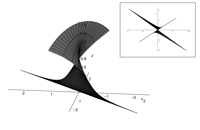
Figure 1: ‘Rotating‘ string in ${AdS}_{5}$ space in Poincare coordinates. This is an Euclidean world-sheet which approaches the boundary at the $x_{3}=t$ line. The results for the anomalous dimension are the same as with the usual rotating string in global coordinates. The inset depicts the projection of the world-sheet onto the boundary on the plane ($x_{3}$,$t$).

As an aside note also that as $\tau$ goes to infinity which is the relevant limit to compute the anomalous dimension, the string extends, as we just said, along the light-like line $x_{3}=t$. It will be interesting to understand if this is in some way related to the Wilson loop calculation which also uses light-like lines in the boundary. On the other hand it seems to be related to the fact that the twist two operators appear in the expansion of a bilocal operator which contains a light-like Wilson line as we see from eq.(12) below.

II.2 Anomalous dimensions from Wilson loops

In gauge field theories there is a way to compute the anomalous dimensions of large spin, twist two operators using Wilson loops Korchemsky and Marchesini (1993); Korchemsky (1989). The argument starts by considering the bilocal operator:

$$W_{\Delta^{\mu}} = \mathop{\rm Tr}\left(\Phi^{I}(\Delta^{\mu})e^{\int_{0}^{1}A_{\mu}(t\Delta^{\mu})\Delta^{\mu}dt}\Phi^{I}(0)\right)=\sum_{S=0}^{\infty}\frac{1}{S!}\mathcal{O}_{S}(\Delta^{\mu}),$$ (11)

$$\mathcal{O}_{S}(\Delta^{\mu}) = \mathop{\rm Tr}\left(\Phi^{I}\nabla_{\mu_{1}}\cdots\nabla_{\mu_{S}}\Phi^{I}\right)\Delta^{\mu_{1}}\cdots\Delta^{\mu_{S}},$$ (12)

where $\Delta^{\mu}$ is a fixed light-like vector and the Wilson line is in the adjoint representation ($A_{\mu}=A^{a}_{\mu}C_{abc}$). The operators $\mathcal{O}_{S}(\Delta^{\mu})$ are the (space-time) component of the operators (I) with maximum helicity along $\Delta^{\mu}$. Matrix elements of this operator require renormalization which give rise to an anomalous dimension. In particular we can compute matrix elements between one particle states of the field $\Phi^{I}$ with momentum $p$. It was observed in Korchemsky and Marchesini (1993); Korchemsky (1989) that the limit $S\rightarrow\infty$ corresponds to $p.\Delta\rightarrow\infty$ and that, in that limit, such matrix elements can be computed using Wilson loops. The relevant Wilson loops have an anomalous dimension due to the fact that they have cusps. Generically, for a Wilson loop with a cusp of angle $\gamma$ the expectation value behaves as Polyakov (1980):

$$W_{\gamma}\sim\left(\frac{\Lambda}{m}\right)^{-\Gamma_{\mathrm{cusp}}(\gamma)},$$ (13)

where $\Lambda$ is an UV cutoff. In our case it turns out that $\gamma\simeq\ln(p.\Delta)$ which diverges for $p.\Delta\rightarrow\infty$. In such regime the cusp anomaly behaves as Korchemsky and Radyushkin (1987):

$$\Gamma_{\mathrm{cusp}}(\gamma)\simeq\bar{\Gamma}_{\mathrm{cusp}}\gamma,\ \ \ \gamma\rightarrow\infty.$$ (14)

Using this result one can see that the anomalous dimension is given by:

$$\Delta_{S}-S-2=\gamma_{S}\simeq-2\bar{\Gamma}_{\mathrm{cusp}}\ln S,\ \ \ \ (S\rightarrow\infty).$$ (15)

What is left now is to compute $\bar{\Gamma}_{\mathrm{cusp}}$. To summarize, one should compute a Wilson loop with the shape of a wedge such as that in fig.2 where both sides approach the light-like lines $x=\pm t$, $t>0$. In that limit the expectation value should behave as in (13) with $\Gamma_{\mathrm{cusp}}$ as in eq.(14). After extracting the constant $\bar{\Gamma}_{\mathrm{cusp}}$, we can use (15) and get the anomalous dimension. A Wilson loop as that in fig.2 can be computed by using a surface of minimal area in ${AdS}_{5}$ with metric

$$ds^{2}=\frac{R^{2}}{z^{2}}\left(dz^{2}-dt^{2}+dx_{1}^{2}+dx_{2}^{2}+dx_{3}^{2}\right),$$ (16)

and ending at $z=0$ on the lines $x=\pm t$, $t>0$. Such surface turns out to be given simply by the equation $z^{2}=2(t^{2}-x^{2})$. The area $\mathcal{A}$ of such surface is divergent but we can regulate it as:

$$\mathcal{A}=\frac{R^{2}}{2\pi\alpha^{\prime}}\frac{1}{2}\int_{0}^{\infty}\frac{d\rho}{\rho}\int_{-\infty}^{+\infty}d\xi=\frac{R^{2}}{2\pi\alpha^{\prime}}\frac{1}{2}\int_{\epsilon}^{L}\frac{d\rho}{\rho}\int_{-\gamma/2}^{+\gamma/2}d\xi=\frac{R^{2}}{2\pi\alpha^{\prime}}\frac{1}{2}\gamma\ln\frac{L}{\epsilon},$$ (17)

which, using that $\mathcal{A}=\ln W$, $\Lambda\sim 1/\epsilon$ and $R^{2}/\alpha^{\prime}=\sqrt{g_{s}N}$ implies that $\bar{\Gamma}_{\mathrm{cusp}}=-\sqrt{g_{s}N}/4\pi$. This calculation is actually for a Wilson loop in the fundamental. Since we need a Wilson loop in the adjoint we should multiply the result by a factor of two. Taking this into account and using formula (15) we obtain the conformal dimension

$$\Delta_{S}\simeq S+\frac{\sqrt{g_{s}N}}{\pi}\ln S,\ \ \ \ \ (S\rightarrow\infty).$$ (18)

Actually, the surface $z^{2}=2(t^{2}-x^{2})$ has a simple expression in embedding coordinates which can be obtained from symmetry arguments alone. A comment is that one can be more rigorous and find a surface ending on two space-like lines and take the limit in which they become light-like obtaining the same result.

The fact that the anomalous dimension behaves as $\ln S$ for large $S$ depends on the fact that the cusp anomaly $\Gamma_{\mathrm{cusp}}(\gamma)$ diverges linearly in $\gamma$ for large $\gamma$. In the Wilson loop calculation this follows from the fact that the integrand in eq.(17) does not depend on $\xi$ which is a consequence of Lorentz invariance. It is interesting to observe that the fact that the anomalous dimension behaves as $\ln S$ Korchemsky and Radyushkin (1987) appears as a consequence of Lorentz invariance also in the field theory calculation.

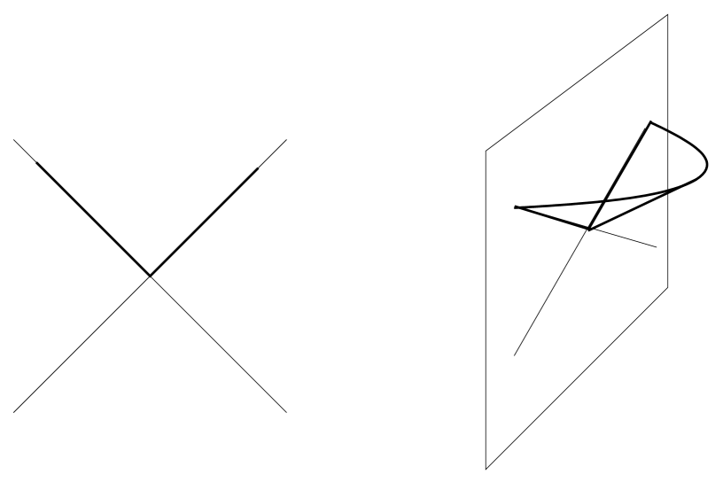
Figure 2: Light-like Wilson loop used to compute the anomalous dimension and the corresponding surface in ${AdS}_{5}$. Thin lines indicate the light-cone. This Wilson loop is actually singular but can be used to compute the limit of a space-like one since the ${AdS}_{5}$ surface is well defined.

It is also interesting to note that the symmetries determine the behavior of the cusp anomaly for small Euclidean angles. In fact, the flat metric $ds^{2}=dr^{2}+r^{2}d\theta^{2}$, is invariant (up to a conformal factor) under the transformation $r\rightarrow r^{\lambda}$, $\theta\rightarrow\lambda\theta$. When $\Theta\rightarrow 0$ we can ignore the fact that such a transformation alters the periodicity of $\theta$ and obtain that $\ln W_{M}\sim-\Gamma_{\mathrm{cusp}}(\Theta)\ln(L/\epsilon)$ is invariant only if $\Gamma_{\mathrm{cusp}}(\Theta)\sim 1/\Theta(\Theta\rightarrow 0)$. From supergravity we get

$$\Gamma_{\mathrm{cusp}}(\Theta)\simeq-\frac{R^{2}}{2\pi\alpha^{\prime}}\frac{c^{2}}{\Theta},\ \ \ \ (\Theta\rightarrow 0).$$ (19)

with the expected behavior $1/\Theta$. The constant $c$ is given by Kruczenski (2002):

$$c=\int_{-\infty}^{\infty}\frac{du}{(1+u^{2})^{3/2}(2+u^{2})^{1/2}}=\frac{(2\pi)^{\frac{3}{2}}}{\left(\Gamma(\frac{1}{4})\right)^{2}}.$$ (20)

We can also compute the same result by using the quark anti-quark potential $V(L)$ which was computed in Maldacena (1998b); Rey and Yee (2001). In fact, when $\Theta\rightarrow 0$ the lines are almost parallel and the Wilson loop should be

$$\ln W\simeq\int_{\epsilon}^{L}d\rho V(\rho)=-\frac{2c_{1}^{2}}{\pi}\sqrt{g_{s}N}\int_{\epsilon}^{L}\frac{d\rho}{\rho\Theta},$$ (21)

and therefore the cusp anomaly is

$$\Gamma_{\mathrm{cusp}}\simeq-\frac{2c_{1}^{2}}{\pi}\sqrt{g_{s}N}\frac{1}{\Theta},$$ (22)

which agrees with eq.(19) if we use (20) and the value $c_{1}=\sqrt{2}\pi^{3/2}/\Gamma(1/4)^{2}$ from Maldacena (1998b); Rey and Yee (2001).

III The Klebanov-Tseytlin background and Cascading theories.

In this section we review the Klebanov-Tseytlin background and its field theory dual.

III.1 Supergravity background

In Klebanov and Tseytlin (2000), I. Klebanov and A. Tseytlin found a type $IIB$, $\mathcal{N}=1$ background with metric

$$ds^{2}=h(r)^{-\frac{1}{2}}dx_{\mu}dx^{\mu}+h(r)^{\frac{1}{2}}ds^{2}_{[6]}=h(r)^{-\frac{1}{2}}dx_{\mu}dx^{\mu}+h(r)^{\frac{1}{2}}\left(dr^{2}+r^{2}ds^{2}_{{\mathbb{T}}^{1,1}}\right),$$ (23)

where $ds^{2}_{[6]}=dr^{2}+r^{2}ds^{2}_{{\mathbb{T}}^{1,1}}$ is a Ricci-flat Kähler metric on the complex cone $w_{1}^{2}+w_{2}^{2}+w_{3}^{2}+w_{4}^{2}=0$, ${\mathbb{T}}^{1,1}$ is a manifold which is the base of the cone and we defined

$$h(r) = \frac{1}{r^{4}}\left[R^{4}+2L^{4}\left(\ln\frac{r}{r_{0}}+\frac{1}{4}\right)\right],$$ (24)

$$R^{4} = \frac{27}{4}g_{s}N\pi(\alpha^{\prime})^{2},$$ (25)

$$L^{2} = \frac{9}{4}g_{s}M\alpha^{\prime}.$$ (26)

Here $M$ and $N$ are arbitrary parameters of the solution. The RR and NSNS field strengths are given by:

$$F_{[5]} = (1+*_{10})(\partial_{r}h^{-1})d^{4}x\wedge dr,$$ (27)

$$B_{[2]} = \frac{2L^{2}}{3}\ln(r/r_{0})\omega_{[2]},$$ (28)

$$F_{[3]} = \frac{2L^{2}}{9g_{s}}\omega_{[3]},$$ (29)

where $\omega_{[3]}$ and $\omega_{[2]}$ are certain closed forms in ${\mathbb{T}}^{1,1}$ which can be found in Klebanov and Tseytlin (2000); Klebanov and Strassler (2000) and will not be essential to our purpose here.

The complex cone $w_{1}^{2}+w_{2}^{2}+w_{3}^{2}+w_{4}^{2}=0$ can be endowed with a Kähler metric whose Kähler potential depends only on $\sum_{i=1}^{4}w_{i}\bar{w}_{i}$ which is actually the metric $ds^{2}_{[6]}$ we are using. It follows that written in terms of the $w_{i}$ the Kähler potential has an $SU(4)$ symmetry which however is reduced to $SO(4)\times U(1)$ due to the condition $w_{1}^{2}+w_{2}^{2}+w_{3}^{2}+w_{4}^{2}=0$. The $SO(4)$ acts on the indices $i$ and the $U(1)$ symmetry is $w_{i}\rightarrow e^{i\alpha}w_{i}$. This $SO(4)\times U(1)$ is therefore an isometry of the metric (23). The $U(1)$ however is not a symmetry Klebanov et al. (2002) because, in spite of being an isometry, it does not leave invariant the RR potential $C_{[2]}$ ($F_{[3]}=dC_{[2]}$). This corresponds in the field theory to a chiral anomaly that breaks the $U(1)$ to ${\mathbb{Z}}_{2M}$. In fact, at low energies we expect the appearance of a gluino condensate which breaks this further to ${\mathbb{Z}}_{2}$. In supergravity this is reflected in the fact that the solution (23) is singular at $r=r_{0}$. The appropriate, non singular metric is the Klebanov Strassler (KS) background Klebanov and Strassler (2000) where from the original $U(1)$ isometry only a ${\mathbb{Z}}_{2}$ subgroup remains. This happens because for $ds_{[6]}^{2}$ one uses a metric on the deformed conifold $w_{1}^{2}+w_{2}^{2}+w_{3}^{2}+w_{4}^{2}=\epsilon^{2}$, $\epsilon\neq 0$. The 10-dimensional KS metric can be written as Klebanov and Strassler (2000)

$$ds^{2} = h(\mathcal{T})^{-\frac{1}{2}}dx_{\mu}dx^{\mu}+h(\mathcal{T})^{\frac{1}{2}}ds^{2}_{[6]}$$ (30)

$$= h(\mathcal{T})^{-\frac{1}{2}}dx_{\mu}dx^{\mu}+h(\mathcal{T})^{\frac{1}{2}}\left[\frac{\epsilon^{\frac{4}{3}}}{6}\frac{1}{K(\mathcal{T})^{2}}d\mathcal{T}^{2}\right]+ds_{[5]}^{2},$$ (31)

where we denoted the new radial coordinate as $\mathcal{T}$. Also, $ds^{2}_{[6]}$ is now a Ricci flat, Kähler metric on the deformed conifold, $ds^{2}_{[5]}$ is a ($\mathcal{T}$-dependent) metric on a deformed ${\mathbb{T}}^{1,1}$. The functions $K(\mathcal{T})$ and $h(\mathcal{T})$ can be obtained by solving the equations of motion but will not be of interest here since we will need only the limit $\mathcal{T}\rightarrow\infty$ where this metric reduces to (23).

Going back to the metric (23) we can observe that it is similar to $AdS_{5}\times{S}^{5}$ but with $S^{5}$ replaced by ${\mathbb{T}}^{1,1}$. Also, in ${AdS}_{5}$ we have $h(r)=R^{4}/r^{4}$. Comparing with (24) we see that we can pictorially describe the background as ${AdS}_{5}$ with a (logarithmically) $r$ dependent radius $R(r)$. One can also define a radial dependent $N_{\mathrm{eff.}}(r)$ by integrating the $5$-form flux over ${\mathbb{T}}^{1,1}$ and obtaining

$$N_{\mathrm{eff.}}=N+\frac{3}{2\pi}g_{s}M^{2}\ln\frac{r}{r_{0}}.$$ (32)

Since we know that $AdS_{5}\times{S}^{5}$ with $N$ units of 5-form flux describe a theory with $N^{2}$ degrees of freedom, these qualitative considerations lead one to consider that the effective number of degrees of freedom changes with the radius, and therefore with the scale. This idea has actually been supported by thermodynamic arguments Buchel (2001); Buchel et al. (2001); Gubser et al. (2001) and from the analysis of $2$-point functions in this background Krasnitz (2002, 2000). We should point out that since the KT background is singular at $r=r_{0}$, the KS (which resolves the singularity) is necessary to understand the infrared properties of the theory but, since we are interested in the UV properties of the theory, which correspond to $r\rightarrow\infty$ and both backgrounds behave similarly in that region, we can use the simpler background (23).

III.2 Cascading field theory

The dual field theory to (23) was suggested in Klebanov and Tseytlin (2000) and made precise in Klebanov and Strassler (2000). It was argued that the dual field theory can be described by a set of theories, each valid at a certain energy scale, which are $\mathcal{N}=1$ gauge theories with gauge group $SU(N)\times SU(N+M)$. Each theory is given by a different $N(\mu)$ and is valid at a certain energy scale $\mu$.

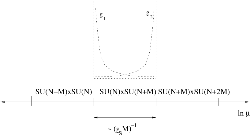
Figure 3: Cascading theory.

Each theory has the field content of pure $\mathcal{N}=1$ SYM with gauge group $SU(N)\times SU(N+M)$ plus a pair of chiral multiplets $A_{i=1,2}$ in the $(N,\overline{N+M})$ and another pair $B_{i=1,2}$ in the $(\bar{N},N+M)$. The global symmetry is $SU_{A}(2)\times SU_{B}(2)\times U_{B}(1)$ where the $SU_{A}(2)$ rotates the $A_{i=1,2}$ fields and $SU(2)_{B}$ rotates the $B$’s. The coupling constants of the two gauge groups run as Klebanov and Tseytlin (2000); Klebanov and Strassler (2000)

$$\frac{8\pi^{2}}{g^{2}_{N+M}} = 3M\ln\left(\frac{\mu}{\mu_{1}}\right)+\mathcal{O}(\frac{M^{2}}{N^{2}}),\ \ \ \ \mu>\mu_{1},$$ (33)

$$\frac{8\pi^{2}}{g^{2}_{N}} = 3M\ln\left(\frac{\mu_{2}}{\mu}\right)+\mathcal{O}(\frac{M^{2}}{N^{2}}),\ \ \ \ \mu<\mu_{2}.$$ (34)

We see that the $SU(N+M)$ gauge theory is asymptotically free whereas the $SU(N)$ is IR free. The perturbative description is valid only for scales $\mu$ such that $\mu_{1}<\mu<\mu_{2}$. For $\mu<\mu_{1}$ the $SU(N+M)$ gauge theory becomes strongly coupled and its correct description is in terms of a Seiberg dual theory Seiberg (1995) with gauge group $SU(N-M)$, i.ethe gauge group is now $SU(N-M)\times SU(N)$. For $\mu>\mu_{2}$ the gauge group $SU(N)$ is dualized to $SU(N+2M)$. It is interesting that a careful application of Seiberg duality shows that the dual theories have similar field content. We obtain in this way a cascade of theories which are the same except for the change in the gauge group (we summarize the situation in fig.3). It is meaningful then to define a scale dependent $N$. The dependence is such that $N$ changes by $M$ in the interval $\mu_{1}<\mu<\mu_{2}$. We get then

$$\frac{\Delta N}{\Delta\ln\mu}=\frac{M}{\ln\frac{\mu_{2}}{\mu_{1}}}.$$ (36)

Using (LABEL:betafunctions) and the supergravity relation Klebanov and Strassler (2000)

$$\frac{8\pi^{2}}{g_{N+M}^{2}}+\frac{8\pi^{2}}{g_{N}^{2}}=\frac{2\pi}{g_{s}},$$ (37)

we get

$$\frac{8\pi^{2}}{g_{N+M}^{2}}+\frac{8\pi^{2}}{g_{N}^{2}}=3M\ln\frac{\mu_{2}}{\mu_{1}}=\frac{2\pi}{g_{s}}\ \ \Rightarrow\ \ \ln\frac{\mu_{2}}{\mu_{1}}=\frac{\pi}{3Mg_{s}},$$ (38)

and therefore eq.(36) becomes

$$\frac{\Delta N}{\Delta\ln\mu}=\frac{M}{\ln\frac{\mu_{2}}{\mu_{1}}}=\frac{3M^{2}g_{s}}{2\pi}.$$ (39)

In the limit where $g_{s}M^{2}\ll N$ it is appropriate to define a continuously varying $N$ which can be obtained by integrating the previous relation:

$$N(\mu)=N_{0}+\frac{3}{2\pi}g_{s}M^{2}\ln\frac{\mu}{\mu_{0}},$$ (40)

in exact agreement with the supergravity result (32). Furthermore since we are describing the theory with a continuously varying $N$ it only makes sense to study operators which are, in a certain sense, self dual under the Seiberg dualities. We can call them operators that cascade nicely. One such type of operator is

$$\mathop{\rm Tr}\left(A_{i}(x)B_{j}(x)\right).$$ (41)

This operator becomes a meson operator under Seiberg duality. In this case however Klebanov and Strassler (2000), meson operators are massive and can be integrated out with the result that the operator dualizes (up to factors) into

$$\mathop{\rm Tr}\left(a_{i}(x)b_{j}(x)\right),$$ (42)

where $a_{i}$ and $b_{j}$ are the chiral superfields of the dual theory. In this sense the operator cascades nicely.

IV Light-like wedges in the KT-background

As we explained in section II.2, the anomalous dimension of twist two operators can be computed by finding a surface in the bulk which ends on a light-like wedge in the boundary. In order to do this it is convenient to write the metric (23) using Rindler coordinates ($\rho,\xi$) in the plane ($t,x_{3}$):

$$ds^{2}=h(r)^{-\frac{1}{2}}\left(-d\rho^{2}+\rho^{2}d\xi^{2}+dx_{1}^{2}+dx_{2}^{2}\right)+h(r)^{\frac{1}{2}}\left(dr^{2}+r^{2}ds^{2}_{{\mathbb{T}}^{1,1}}\right).$$ (43)

The surface in question is given by a function $r(\rho,\xi)$ which minimizes the world-sheet action. Lorentz invariance however implies that $r$ is a function only of $\rho$:

$$r(\rho,\xi)\stackrel{{\scriptstyle\mathrm{Lorenz\ inv.}}}{{\longrightarrow}}r(\rho).$$ (44)

The action that we should minimize becomes then

$$S=\frac{1}{2\pi\alpha^{\prime}}\int d\xi\int\rho d\rho\sqrt{r^{\prime 2}-h^{-1}}=\frac{1}{2\pi\alpha^{\prime}}\int d\xi\int\rho(r)\sqrt{1-\rho^{\prime 2}/h(r)}dr,$$ (45)

where we find convenient to solve for $\rho(r)$ instead of $r(\rho)$. At this point we should replace $h(r)$ for its value from (24):

$$h(r)=\frac{1}{R^{4}}\left[R^{4}+\frac{1}{2}L^{4}+2L^{4}\ln\frac{r}{r_{0}}\right]=\frac{2L^{4}}{r^{4}}\ln\frac{r}{\tilde{r}_{0}},$$ (46)

where, for concision, we introduced $\tilde{r}_{0}$ defined through

$$\ln\frac{r_{0}}{\tilde{r}_{0}}=\frac{R^{4}}{2L^{4}}+\frac{1}{4}.$$ (47)

It turns out to be useful to introduce also the definitions

$$r=\tilde{r}_{0}e^{\zeta},\ \ \ \ \tilde{\rho}=\frac{\tilde{r}_{0}}{\sqrt{2}L^{2}}\rho.$$ (48)

The action becomes

$$S=\frac{\sqrt{2}L^{2}}{2\pi\alpha^{\prime}}\int d\xi\int d\zeta e^{\zeta}\tilde{\rho}\sqrt{1-\frac{1}{\zeta}e^{2\zeta}\left(\frac{d\tilde{\rho}}{d\zeta}\right)^{2}}.$$ (49)

From here we obtain the equation of motion:

$$-\frac{d}{d\zeta}\left[\frac{\tilde{\rho}e^{3\zeta}}{\zeta\sqrt{1-\frac{1}{\zeta}e^{2\zeta}\left(\frac{d\tilde{\rho}}{d\zeta}\right)^{2}}}\left(\frac{d\tilde{\rho}}{d\zeta}\right)\right]=e^{\zeta}\sqrt{1-\frac{1}{\zeta}e^{2\zeta}\left(\frac{d\tilde{\rho}}{d\zeta}\right)^{2}}.$$ (50)

This equation cannot be solved analytically but we are interested actually in the behavior for $r\rightarrow\infty$, i.e$\zeta\rightarrow\infty$ because that is the UV region which determines the anomalous dimensions. In that region we will be able to obtain an asymptotic series expansion of the solution which can be complemented by a numerical analysis. Before that however let us analyze the properties of the equation. To do that it is useful to introduce a new variable $x$ and function $y(x)$ through

$$\tilde{\rho}=e^{-\zeta}\sqrt{\zeta}\frac{1}{\sqrt{2}}y(x),\ \ \ \ \ x=\frac{1}{\zeta}.$$ (51)

The resulting equation for $y(x)$ can be written as

$$y^{\prime\prime}(x)=\frac{1}{yx^{4}}P(x,y,y^{\prime}),$$ (52)

where $P(x,y,y^{\prime})$ is a polynomial given by

$$P(x,y,y^{\prime}) = -(y^{2}-1)(y^{2}-2)+\left(-\frac{5}{2}+\frac{7}{4}y^{2}\right)y^{2}x+\left(3y^{\prime}-\frac{9}{8}y^{3}-3y^{2}y^{\prime}+y\right)yx^{2}$$ (53)

$$+\left(\frac{15}{4}y^{2}y^{\prime}-3y^{\prime}+\frac{5}{16}y^{3}\right)yx^{3}+\left(-\frac{3}{2}\,{y}^{3}{y^{\prime}}-3\,{y}^{2}{{y^{\prime}}}^{2}+{{y^{\prime}}}^{2}-\frac{1}{32}\,{y}^{4}\right){x}^{4}$$

$$+\left(\frac{9}{4}y^{\prime 2}+\frac{3}{16}yy^{\prime}\right)y^{2}x^{5}+\left(-y^{\prime 3}-\frac{3}{8}yy^{\prime 2}\right)yx^{6}+\frac{1}{4}\,yy^{\prime 3}x^{7}.$$

Although the actual expression for the polynomial is not very illuminating the point is that in the form (52) it is clear that the equation has no singular points except at $x=0$ and $y=0$. That means that around any value $x_{0}\neq 0$ we can find a solution with given initial arbitrary values $y(x_{0})\neq 0$ and $y^{\prime}(x_{0})$. This solution can be found numerically or in a power series expansion that converges in a neighborhood of $x_{0}$. On the other hand we are interested in the region $\zeta\rightarrow\infty$ that corresponds to $x\rightarrow 0$, namely the behavior near the singularity. If we expand $P(x,y,y^{\prime})$ for small $x$ we get

$$P(x,y,y^{\prime})=-(y^{2}-1)(y^{2}-2)+\mathcal{O}(x),$$ (54)

which means that if we want $y^{\prime\prime}(x)$ (and $y(x)$) to stay finite as $x\rightarrow 0$, we need (from eq.(52)) that $y(0)=\pm 1$ or $y(0)=\pm\sqrt{2}$. We will see later on that $y(0)=\pm\sqrt{2}$ corresponds to a light-like surface whereas $y(0)=\pm 1$ corresponds to the Euclidean surface we are looking for. In the $\mathcal{N}=4$ case in Poincare coordinates, this correspond to having the surfaces $z^{2}=t^{2}-x^{2}$ and $z^{2}=2(t^{2}-x^{2})$, the latter being the relevant one. After we choose $y(0)=1$ the next step is to observe that $y^{\prime}(0)$ is also determined if the solution is not to be singular and so on. In that way we get the asymptotic expansion

$$y(x)=\left[1+\frac{3}{8}\,x-\frac{13}{128}\,x^{2}+\frac{127}{1024}\,x^{3}-\frac{5085}{32768}x^{4}+\ldots\right]+\mathcal{O}\left(e^{-\sqrt{2}/x}\right).$$ (55)

Within the square parenthesis we have an infinite series all whose coefficients are completely determined. To this, an arbitrary function of order $\mathcal{O}\left(e^{-\sqrt{2}/x}\right)$ can be added. This function has all its derivatives equal to zero and cannot be derived from the condition of finiteness at $x=0$. It is determined by the initial conditions. That this has to be the case is clear from the previous discussion. For each initial point $x_{0}$ we have a two parameter family of solutions parameterized by $y(x_{0})$ and $y^{\prime}(x_{0})$. The condition of finiteness at $x=0$ gives a relation between $y(x_{0})$ and $y^{\prime}(x_{0})$ but there is still a one parameter family of solutions regular at $x=0$. What we stated above is that all those solutions have the asymptotic behavior (55) up to exponentially suppressed terms. We can verify this numerically by plotting different solutions and comparing with eq.(55). We do that in fig.4 where we plotted $y(\zeta)$ for $y(1)=1.16837534663212$, $y^{\prime}(1)=0$ and $y(1)=0.7381269451991$, $y^{\prime}(1)=1$ together with the function (55) after changing variables $x=1/\zeta$. We see that the three function have the same asymptotic behavior, the difference can also be computed and agrees with the analytical result that it is exponentially suppressed. This estimate follows from expanding the polynomial $P$ around $x=0$, $y=1$ which gives

$$y\simeq 1+\delta y,\,\,\,\mbox{with}\ \ \ \ x^{4}\,\delta y^{\prime\prime}-2\,\delta y=-\frac{3}{4}x.$$ (56)

The linear equation for $\delta y$ (together with the condition of $\delta y$ finite at $x=0$) can be exactly solved:

$$\delta y=\frac{3}{8}x+C_{1}xe^{-\sqrt{2}/x}.$$ (57)

From here we get the value $y^{\prime}(0)=3/8$. The constant $C_{1}$ is arbitrary since it multiplies a solution of the homogeneous equation and corresponds to the arbitrary function that we mentioned before has to be determined by the initial conditions. This initial conditions should follow from the IR of the background but as we see are not relevant as long as we discard the exponentially suppressed terms.

Figure 4: The solid line $(1)$ depicts the function (55) after changing variables to $\zeta=1/x$. The other two are numerical solution to eq.(52) with initial conditions ($y(1)=1.16837534663212$, $y^{\prime}(1)=0$) for curve $(2)$ and ($y(1)=0.7381269451991$, $y^{\prime}(1)=1$) for curve $(3)$. Again we are using $\zeta=1/x$ as the independent variable. The initial conditions are chosen such that both functions are finite at $\zeta\rightarrow\infty$ in which case their asymptotic behavior is seen to be well described by the solid line, namely eq.(55).

Going back to eq.(50) we find, from (55) and (51) that the asymptotic solution is

$$\tilde{\rho}(\zeta)\sim e^{-\zeta}\sqrt{\zeta}\frac{1}{\sqrt{2}}\left[1+\frac{3}{8}\,\frac{1}{\zeta}-\frac{13}{128}\,\frac{1}{\zeta^{2}}+\frac{127}{1024}\,\frac{1}{\zeta^{3}}-\frac{5085}{32768}\frac{1}{\zeta^{4}}+\ldots\right].$$ (58)

The previous discussion was mainly to understand the properties of the equation and what the asymptotic expansion means. For the purpose of computing the anomalous dimension we will keep only the first term which gives, after replacing in the action

$$\left.\begin{array}[]{lcl}\tilde{\rho}&\simeq&e^{-\zeta}\frac{\sqrt{\zeta}}{\sqrt{2}}\\ \frac{d\tilde{\rho}}{d\zeta}&\simeq&-e^{-\zeta}\frac{\sqrt{\zeta}}{\sqrt{2}}\end{array}\right\}\ \ \Rightarrow\ \ S\simeq\frac{\sqrt{2}L^{2}}{2\pi\alpha^{\prime}}\int d\xi\int d\zeta\frac{\sqrt{\zeta}}{\sqrt{2}}\sqrt{1-\frac{1}{2}}.$$ (59)

If we had chosen $y(0)=\sqrt{2}$, inside the square root we would have got $\sqrt{1-1}=0$, namely a light-like surface as we said before. We can regulate the integrals in the action in the same manner as for the $\mathcal{N}=4$ case, integrating the angle $\xi$ between $-\gamma/2$ and $\gamma/2$ with $\gamma\rightarrow\infty$ and $\zeta$ between $0$ and $\zeta_{m}$:

$$S=\frac{L^{2}}{2\pi\alpha^{\prime}\sqrt{2}}\int_{-\gamma/2}^{\gamma/2}d\xi\int_{0}^{\zeta_{m}}d\zeta\sqrt{\zeta}=\frac{L^{2}}{2\pi\alpha^{\prime}\sqrt{2}}\gamma\frac{2}{3}\zeta_{m}^{\frac{3}{2}}.$$ (60)

The parameter $\zeta_{m}$ should be understood as a UV cutoff since $\zeta=\ln(r/\tilde{r}_{0})$ and then $\zeta<\zeta_{m}$ is the same as $r<r_{m}=\tilde{r}_{0}\exp(\zeta_{m})$. In the cascade theory, if the steps of the cascade are large ($g_{s}M^{2}\sim N$) then one can introduce a UV cut-off for each theory (e.g$\mu_{2}$ in our previous notation) but in the limit ($g_{s}M^{2}\ll N$) the steps of the cascade are small and the cutoff should be better understood as the energy scale $\mu$ at which we probe the cascade which just determines the value of $N_{\mbox{eff.}}(\mu)$ that we have to use. Then we identify $\zeta_{m}=\ln(\mu/\mu_{0})$ where we identified $r\sim\mu$ up to a constant. We get then

$$S=\ln W=\frac{L^{2}}{2\pi\alpha^{\prime}\sqrt{2}}\gamma\frac{2}{3}\left(\ln\frac{\mu}{\mu_{0}}\right)^{\frac{3}{2}}.$$ (61)

Now we appeal to the definition of anomalous dimension

$$\mu\frac{\partial W}{\partial\mu}=-\Gamma_{\mathrm{cusp}}W,$$ (62)

and get

$$\Gamma_{\mathrm{cusp}}=-\frac{L^{2}}{2\pi\alpha^{\prime}\sqrt{2}}\gamma\left(\ln\frac{\mu}{\mu_{0}}\right)^{\frac{1}{2}},$$ (63)

which is linear in $\gamma$ as expected from Lorentz invariance. The proportionality coefficient is $\bar{\Gamma}_{\mathrm{cusp}}$:

$$\bar{\Gamma}_{\mathrm{cusp}}=-\frac{L^{2}}{2\pi\alpha^{\prime}\sqrt{2}}\left(\ln\frac{\mu}{\mu_{0}}\right)^{\frac{1}{2}},$$ (64)

from where the Korchemsky-Marchesini formula (15) gives the anomalous dimension

$$\gamma(\mu)=2\frac{L^{2}}{\pi\alpha^{\prime}\sqrt{2}}\left(\ln\frac{\mu}{\mu_{0}}\right)^{\frac{1}{2}}\ln S=\frac{3\sqrt{3}}{2}\frac{1}{\sqrt{\pi}}\sqrt{g_{s}N_{\mbox{eff.}}}\ln S,$$ (65)

where the extra factor of two appears because the Wilson loop should actually be in the adjoint (twice the fundamental). In the second equality we used the definition (26). This anomalous dimension is the main result of this section and of the paper. In the next section we reproduce it using rotating strings. The important difference with the $\mathcal{N}=4$ case is that the theory is not conformally invariant and so the anomalous dimension depends on the scale and we have to use the appropriate definition of anomalous dimension as eigenvalues under infinitesimal scale transformations (62). Incidentally taking the derivative (62) provides a factor $3/2$ that makes the result agree with the rotating string calculation.

V Rotating string version

Here we do the rotating string calculation equivalent to the Wilson loop calculation of the previous section. For that we will first consider the KS background (31)

$$ds^{2}=h^{-\frac{1}{2}}(\mathcal{T})(-dt^{2}+dx_{1}^{2}+dx_{2}^{2}+dx_{3}^{3})+h^{\frac{1}{2}}(\mathcal{T})\frac{\varepsilon^{\frac{4}{3}}}{6}\frac{1}{K^{2}(\mathcal{T})}d\mathcal{T}^{2}+ds_{5}^{2}(\mathcal{T}).$$ (66)

We can do a coordinate transformation

$$z=\int_{\mathcal{T}}^{\infty}\frac{\varepsilon^{\frac{4}{3}}}{6}\frac{h(\mathcal{T})}{K^{2}(\mathcal{T})},$$ (67)

to render the metric into the form

$$ds^{2}=h^{-\frac{1}{2}}(\mathcal{T}(z))(dz^{2}-dt^{2}+dx_{1}^{2}+dx_{2}^{2}+dx_{3}^{3})+ds_{5}^{2}(\mathcal{T}(z)).$$ (68)

Now the same coordinate transformation as in (6) results in the metric:

$$ds^{2} = h^{-\frac{1}{2}}(\mathcal{T}(\frac{e^{-\tau}}{\cosh(\rho)}))\frac{e^{-2\tau}}{\cosh^{2}\rho}\left[\cosh^{2}\rho d\tau^{2}+d\rho^{2}+\sinh^{2}\rho d\phi^{2}+\sinh^{2}\rho\sin^{2}\phi d\theta^{2}\right.$$ (70)

$$\left.-\sinh^{2}\rho\cos^{2}\phi d\chi^{2}\right]+ds_{5}^{2}(\tau,\rho).$$

Naturally it is difficult to find the equivalent solution to that of eq.(II.1) in this background. However since we are interested in the asymptotic properties of the string in the UV, this corresponds to taking $\mathcal{T}\rightarrow\infty$ and we can use the Klebanov-Tseytlin solution. Using a new radial coordinate $r=3^{\frac{1}{2}}2^{-\frac{5}{6}}\epsilon^{\frac{2}{3}}e^{\frac{\tau}{3}}$ and after an appropriate identification of the constants, we recover the metric (23). The transformation (67) becomes

$$z=\int^{r}h(r)^{\frac{1}{2}}dr\simeq\frac{\sqrt{2}L^{2}}{r}\left(\ln\frac{r}{\tilde{r}_{0}}\right)^{\frac{1}{2}},\ \ \ \ (r\rightarrow\infty),$$ (71)

where the last equality is valid for large $r$ and we used that, as before, $h(r)$ is given by

$$h(r)=\frac{2L^{4}}{r^{4}}\ln\frac{r}{\tilde{r}_{0}}.$$ (72)

Note that since $\cosh\rho>1$ and $z=e^{-\tau}/\cosh\rho$ the string never extends beyond $z=e^{-\tau}$, namely, we do not need to know the IR part of the background if $\tau\gg 1$. In this limit, and taking into account that the string does not extend into $x_{1,2}$ or the internal coordinates we can write the relevant part of the metric as

$$ds^{2}\simeq z^{2}h^{-\frac{1}{2}}\left(\cosh^{2}\rho d\tau^{2}+d\rho^{2}-\sinh^{2}\rho d\chi^{2}\right).$$ (73)

Now we compute, at leading order for large $r$ (or large $\tau$):

$$z^{2}h^{-\frac{1}{2}} \simeq \sqrt{2}L^{2}\left(\ln\frac{r}{\tilde{r}_{0}}\right)^{\frac{1}{2}}\simeq\sqrt{2}L^{2}\left(-\ln z\right)^{\frac{1}{2}}$$ (74)

$$= \sqrt{2}L^{2}\left(\ln(e^{-\tau}/\cosh\rho)\right)^{\frac{1}{2}}=\sqrt{2}L^{2}\left(\tau+\ln\cosh\rho\right).$$ (75)

Within this approximation the metric becomes

$$ds^{2}=\sqrt{2}L^{2}\sqrt{\ln(\cosh\rho)+\tau}\left(\cosh^{2}\rho d\tau^{2}+d\rho^{2}-\sinh^{2}\rho d\chi^{2}\right).$$ (76)

As a further approximation we can use that for $\tau\rightarrow\infty$, we have $\tau\gg\ln(\cosh\rho)$ since $\rho<\rho_{0}$ and $\rho_{0}$ is fixed. So we finally get

$$ds^{2}=\sqrt{2}L^{2}\sqrt{\tau}\left(\cosh^{2}\rho d\tau^{2}+d\rho^{2}-\sinh^{2}\rho d\chi^{2}\right).$$ (77)

As a last approximation we note that $\frac{d}{d\tau}\sqrt{\tau}=1/\sqrt{\tau}\rightarrow 0$ and then an adiabatic approximation where $\tau$ is considered constant is appropriate (for large $\tau$). In this case we can define a $\tau$-dependent momentum $P_{\tau}$ which is the bulk equivalent of the fact that the anomalous dimension runs with the scale. Namely, the theory is not scale invariant, but we can define for each scale a conformal dimension that contains the information of how an operator changes under an infinitesimal scale transformation. This conformal dimension is scale dependent because $P_{\tau}$ is $\tau$-dependent.

If we consider $\tau$ constant the calculation becomes the same calculation that we did in section II.1 but after replacing $R^{2}\rightarrow\sqrt{2}L^{2}\sqrt{\tau}$ in the metric (7). This gives (9) with the same replacement $R^{2}\rightarrow\sqrt{2}L^{2}\sqrt{\tau}$:

$$\Delta\simeq S+\frac{\sqrt{2}L^{2}}{\pi\alpha^{\prime}}\sqrt{\tau}\ln S,\ \ \ \ \ (S\rightarrow\infty).$$ (78)

Since at leading order we have $\ln r=\tau$ and we identify $r$ with the scale $\mu$ the result reads

$$\Delta=\frac{2L^{2}}{\pi\alpha^{\prime}}\left(\ln\frac{\mu}{\mu_{0}}\right)^{\frac{1}{2}}\ln S=\frac{3\sqrt{3}}{2}\frac{1}{\sqrt{\pi}}\sqrt{g_{s}N_{\mbox{eff.}}}\ln S,$$ (79)

in exact agreement with the Wilson loop calculation (65).

VI Field theory interpretation

In the previous two sections we used the method of Wilson loops and the one of rotating strings to compute anomalous dimensions of certain field theory operators. In this section we discuss in more detail which are the operators involved. A related discussion already appeared in Buchel (2003). The first point is that since we are in the regime where the steps of the cascade are small compared to $N$, the cascade should be considered as a continuum of theories. In that case the only operators that make sense are those that cascade nicely, that is that can be defined at each step of the cascade and preserve their form under the Seiberg dualities.

In section III we studied the operators

$$\mathcal{O}_{ij}=\mathop{\rm Tr}\left(A_{i}(x)B_{j}(x)\right).$$ (80)

They can be generalized to bilocal operators:

$$\mathcal{O}_{ij}(\Delta_{\mu})=\mathop{\rm Tr}\left(A_{i}(x+\Delta)e^{\int_{x}^{x+\Delta}(A^{(M+N)}_{\mu}+A^{(N)}_{\mu})dx^{\mu}}B_{j}(x)\right),$$ (81)

where we inserted a Wilson line in the bi-fundamental of $SU(N+M)\times SU(N)$ to preserve gauge invariance. These operators should cascade to

$$\mathcal{O}_{ij}(\Delta_{\mu})=\mathop{\rm Tr}\left(a_{i}(x+\Delta)e^{\int_{x}^{x+\Delta}(A^{(M+N)}_{\mu}+A^{(N)}_{\mu})dx^{\mu}}b_{j}(x)\right),$$ (82)

since they are bilocal gauge invariant operators with the same transformation properties under the global symmetry $SU_{A}(2)\times SU_{B}(2)\times U_{B}(1)$. The actual operators that cascade nicely can differ from these ones by functions of the fundamental fields that are invariant under the global symmetries (see Klebanov and Strassler (2000) for a related discussion). We just consider this discussion as evidence of the existence of such operators and use (81) as a guide to understand their properties.

If we expand (81) in powers of $\Delta_{\mu}$ we get a series of operators

$$\mathcal{O}_{ij}(\Delta_{\mu}) = \mathop{\rm Tr}\left(A_{i}(x+\Delta)e^{\int_{x}^{x+\Delta}(A^{(M+N)}_{\mu}+A^{(N)}_{\mu})dx^{\mu}}B_{j}(x)\right)=\sum_{S=0}^{\infty}\frac{1}{S!}\mathcal{O}_{S}^{ij}(\Delta_{\mu}),$$ (83)

$$\mathcal{O}_{S}^{ij}(\Delta_{\mu}) = \mathop{\rm Tr}\left(A_{i}\nabla_{\mu_{1}}\ldots\nabla_{\mu_{S}}B_{j}\right)\Delta^{\mu_{1}}\ldots\Delta^{\mu_{S}}.$$ (84)

If we take, as we did before, $\Delta_{\mu}$ to be light-like then the operators that survive in the contraction are those of maximum helicity, i.e a certain component of the operators of maximum spin that we can form for a given number of derivatives. Since the number of derivatives determines the conformal dimension (in the free theory) these are the operators of lower twist. Note that in that case the Wilson line that appears in eq. (81) is light-like. If one tries to compute such a Wilson line using the AdS/CFT correspondence the natural thing is to use a world-sheet that ends on such a line at the boundary. It is interesting to note that the world-sheet we considered, which appeared as a double Wick rotation of the rotating string has precisely such property. It might be interesting to analyze this point further since a light-like Wilson line is BPS (since its variation involves $\Gamma^{\mu}\Delta_{\mu}$ which satisfies $(\Gamma^{\mu}\Delta_{\mu})^{2}=\Delta^{2}=0$).

Going back to our main point, it is reasonable to suggest that the operators whose anomalous dimension we are computing are precisely $\mathcal{O}_{S}^{ij}$. However, we finalize by pointing out that one can use the vector multiplets to construct other operators which seem to cascade nicely and are invariant under the global symmetries. This is because under Seiberg duality the field strength $W_{\alpha}^{2}$ dualizes to $-\tilde{W}_{\alpha}^{2}$. This operators should be also taken into account if a precise matching between supergravity and the field theory is required. However the supergravity calculation is presently not able to distinguish between all the possible twist two operators. The same happens in the $\mathcal{N}=4$ case where there are several twist two operators (I). The way to distinguish between them is their transformation properties under the global symmetries and supersymmetry. The natural conjecture is that all operators that one can form have the same anomalous dimension for large spin.

VII Conclusions

In this paper we extended previous calculations of anomalous dimensions of twist two operators that were done for $\mathcal{N}=4$ SYM theory to the cascading theories which have $\mathcal{N}=1$ supersymmetry. The interesting difference is that in the $\mathcal{N}=1$ case the anomalous dimension depends on the scale since the theory is not conformally invariant. To tackle the non-conformal case we needed to use a variation of the rotating string method which makes explicit use of the fact that the anomalous dimension is a UV property and then only the UV region of the background should be involved in the calculation. Furthermore we did not use global coordinates since in the non-conformal case there is no state-operator map. In general, a similar calculation done in coordinates akin to global coordinates computes the energy of a certain high spin ‘glueball’ state which is not directly related to the anomalous dimensions of an operator unless the theory is conformally invariant.

Our main interest was in the Wilson loop method that can be easily applied in this case. It makes evident that the logarithmic behavior of the anomalous dimension is a consequence of Lorentz invariance and so seems to be a generic property of all theories that have supergravity duals. In field theory it is known that those are gauge theories since in scalar theories twist two operators have vanishing anomalous dimension in the limit of large spin.

In view of the fact that certain Wilson loops Erickson et al. (2000) can be computed at strong coupling by summing over a subset of Feynman diagrams we believe to be of high interest to see if a similar calculation can give the anomalous dimensions that are obtained from supergravity.

*

Appendix A Coordinates in ${AdS}_{5}$

$AdS_{5}$ has an $SO(4,2)$ isometry group. The isometries are obviously independent of the system of coordinates used, but different systems of coordinates make different isometries manifest (meaning that the coordinates transform simply under a subgroup of the full isometry group) and therefore for different purposes different coordinates are useful.

First consider embedding coordinates. Introducing Cartesian coordinates ($X$, $Y$, $Z$, $W$, $U$, $V$) in ${\mathbb{R}}^{(4,2)}$, ${AdS}_{5}$ is the manifold defined by the equation:

$$-X^{2}-Y^{2}-Z^{2}-W^{2}+U^{2}+V^{2}=R^{2},$$ (85)

for some arbitrary constant $R$. The metric is the one induced by the one in ${\mathbb{R}}^{(4,2)}$:

$$ds^{2}=dX^{2}+dY^{2}+dZ^{2}+dW^{2}-dU^{2}-dV^{2}.$$ (86)

In this (redundant) coordinates, the $SO(4,2)$ isometry group is manifest. More close to the field theory are the Poincare coordinates which parameterize the patch $U+W>0$ and are given by:

$$\begin{array}[]{lll}X=R\,{x_{1}/z},&Y=R\,{x_{2}/z},&Z=R\,{x_{3}/z},\\ W=-{1\over 2z}(-R^{2}+z^{2}+x_{i}^{2}-t^{2}),&U={1\over 2z}(R^{2}+z^{2}+x_{i}^{2}-t^{2}),&V=R\,{t/z},\end{array}$$ (87)

with a metric

$$ds^{2}=\frac{R^{2}}{z^{2}}\left(dz^{2}+dx_{i}^{2}-dt^{2}\right).$$ (88)

In this coordinates we have a manifest $SO(3,1)\times SO(1,1)\subset SO(4,2)$ corresponding to Lorentz transformations and scale transformations $z\rightarrow\lambda z$, $x_{i}\rightarrow\lambda x_{i}$, $t\rightarrow\lambda t$. Scale transformations correspond to boosts along $U,W$ and that is why we denote them as an $SO(1,1)$ subgroup. Operators in the field theory are classified by their spin $(j_{1},j_{2})$ and their conformal dimension $\Delta$.

Global coordinates on the other hand are introduced by splitting the Cartesian coordinates in two groups satisfying:

$$U^{2}+V^{2}=R^{2}\cosh^{2}\rho,\ \ \ \ \ X^{2}+Y^{2}+Z^{2}+W^{2}=R^{2}\sinh^{2}\rho.$$ (89)

For fix $\rho$, the coordinates ($X$,$Y$,$Z$,$W$) span a sphere $S^{3}$ and the coordinates $(U,V)$ a sphere $S^{1}$ which we parameterize with an angle $t$. The metric can then be written as

$$ds^{2}=R^{2}(-\cosh^{2}\!\rho\,dt^{2}+d\rho^{2}+\sinh^{2}\!\rho\,d\Omega_{[3]}^{2}),$$ (90)

where $\Omega_{[3]}$ is the metric of a unit $3$-sphere. They make manifest an $SO(4)\times SO(2)\subset SO(4,2)$ symmetry corresponding to rotations in the $(X,Y,Z,V)$ and $(U,V)$ spaces. These coordinates are convenient because they cover the whole of $AdS_{5}$ space. To relate the eigenvalues under $SO(4)\times SO(2)$ to those of $SO(3,1)\times SO(1,1)$ which are the relevant ones in the field theory we need to do a double Wick rotation such as $V\rightarrow iV$, $W\rightarrow iW$. Under this transformation, the energy, the eigenvalue under $SO(2)$ becomes the conformal dimension, the eigenvalue under $SO(1,1)$.

In this paper we find convenient to introduce another parameterization where the symmetry $SO(3,1)\times SO(1,1)$ is manifest and rotations under $SO(1,1)$ become translations, namely a conserved momentum. In that way no Wick rotation is necessary. To do that we split the embedding coordinates into two groups which are now $(U,W)$ and $(X,Y,Z,V)$ and parameterize this as

$$U^{2}-W^{2}=R^{2}\cosh^{2}\rho,\ \ \ \ \ X^{2}+Y^{2}+Z^{2}-V^{2}=R^{2}\sinh^{2}\rho.$$ (91)

Now, for fixed $\rho$ the coordinates ($X$, $Y$, $Z$, $V$) span a de Sitter space $\Sigma_{[3]}$ and the coordinates ($U$, $W$) a real line which we parameterize with a coordinate $\tau$. With this splitting there is an explicit $SO(1,1)$ isometry corresponding to translations in $\tau$ or equivalently to boosts in the plane ($U$,$W$), and an $SO(3,1)$ isometry which is the isometry group of $\Sigma_{[3]}$. The metric is given by

$$ds^{2}=R^{2}(\cosh^{2}\rho\,d\tau^{2}+d\rho^{2}+\sinh^{2}\rho\,d\Sigma_{[3]}^{2}),$$ (92)

where $d\Sigma^{3}_{[3]}$ is the unit metric on the 3-dimensional de Sitter space $\Sigma_{[3]}$. We see that these coordinates are related to global coordinates by a double Wick rotation: $(t\rightarrow i\tau$, $S^{3}\rightarrow\Sigma_{3}$). This coordinates do not cover the whole space as is evident from the fact that $|U|>|W|$. For the purpose of the paper it is useful to consider coordinates ($\chi$, $\phi$, $\theta$) on $\Sigma_{[3]}$ which together with $\tau$ and $\rho$ parameterize ${AdS}_{5}$ as:

$$\begin{array}[]{lll}U=R\cosh\rho\cosh\tau,&Z=R\sinh\rho\cos\phi\cosh\chi&X=R\sinh\rho\sin\phi\cos\theta,\\ W=R\cosh\rho\sinh\tau,&V=R\sinh\rho\cos\phi\sinh\chi,&Y=R\sinh\rho\sin\phi\sin\theta.\end{array}$$ (93)

The metric is

$$ds^{2}=\cosh^{2}\rho d\tau^{2}+d\rho^{2}+\sinh^{2}\rho d\phi^{2}+\sinh^{2}\rho\sin^{2}\phi d\theta^{2}-\sinh^{2}\rho\cos^{2}\phi d\chi^{2}.$$ (94)

The coordinates chosen cover only part of ${AdS}_{5}$. In particular we see that $U+W>0$ which implies that this coordinate patch is completely contained in the Poincare patch. The relation to Poincare coordinates is easy to work out:

$$\begin{array}[]{lclllcl}x_{1}&=&R\,e^{-\tau}\,\tanh\rho\,\sin\phi\cos\theta&,&x_{2}&=&R\,e^{-\tau}\,\tanh\rho\,\sin\phi\sin\theta,\\ x_{3}&=&R\,e^{-\tau}\,\tanh\rho\,\cos\phi\cosh\chi&,&t&=&R\,e^{-\tau}\,\tanh\rho\,\cos\phi\sinh\chi,\\ z&=&R\,e^{-\tau}\,\frac{1}{\cosh(\rho)}.&&&&\end{array}$$ (95)

We can see now that the $SO(1,1)$ isometry which was given by translations in $\tau$ corresponds to $z\rightarrow\lambda z$, $x_{i}\rightarrow\lambda x_{i}$, namely a scale transformation. So we identify the associated momentum $P_{\tau}$ with the conformal dimension $\Delta=P_{\tau}$. No Wick rotation is necessary in this case.

References

- ’t Hooft (1974a) G. ’t Hooft, Nucl. Phys. B72, 461 (1974a).
- ’t Hooft (1974b) G. ’t Hooft, Nucl. Phys. B75, 461 (1974b).
- Maldacena (1998a) J. M. Maldacena, Adv. Theor. Math. Phys. 2, 231 (1998a), eprint hep-th/9711200.
- Gubser et al. (1998) S. S. Gubser, I. R. Klebanov, and A. M. Polyakov, Phys. Lett. B428, 105 (1998), eprint hep-th/9802109.
- Witten (1998) E. Witten, Adv. Theor. Math. Phys. 2, 253 (1998), eprint hep-th/9802150.
- Aharony et al. (2000) O. Aharony, S. S. Gubser, J. M. Maldacena, H. Ooguri, and Y. Oz, Phys. Rept. 323, 183 (2000), eprint hep-th/9905111.
- Klebanov and Tseytlin (2000) I. R. Klebanov and A. A. Tseytlin, Nucl. Phys. B578, 123 (2000), eprint hep-th/0002159.
- Georgi and Politzer (1974) H. Georgi and H. D. Politzer, Phys. Rev. D9, 416 (1974).
- Gross and Wilczek (1974) D. J. Gross and F. Wilczek, Phys. Rev. D9, 980 (1974).
- Gubser et al. (2002) S. S. Gubser, I. R. Klebanov, and A. M. Polyakov, Nucl. Phys. B636, 99 (2002), eprint hep-th/0204051.
- Axenides et al. (2003) M. Axenides, E. Floratos, and A. Kehagias, Nucl. Phys. B662, 170 (2003), eprint hep-th/0210091.
- Kotikov et al. (2003) A. V. Kotikov, L. N. Lipatov, and V. N. Velizhanin, Phys. Lett. B557, 114 (2003), eprint hep-ph/0301021.
- Kotikov and Lipatov (2003) A. V. Kotikov and L. N. Lipatov, Nucl. Phys. B661, 19 (2003), eprint hep-ph/0208220.
- Kruczenski (2002) M. Kruczenski, JHEP 12, 024 (2002), eprint hep-th/0210115.
- Makeenko (2003) Y. Makeenko, JHEP 01, 007 (2003), eprint hep-th/0210256.
- Belitsky et al. (2003) A. V. Belitsky, A. S. Gorsky, and G. P. Korchemsky, Nucl. Phys. B667, 3 (2003), eprint hep-th/0304028.
- Berenstein et al. (2002) D. Berenstein, J. M. Maldacena, and H. Nastase, JHEP 04, 013 (2002), eprint hep-th/0202021.
- Maldacena (1998b) J. M. Maldacena, Phys. Rev. Lett. 80, 4859 (1998b), eprint hep-th/9803002.
- Rey and Yee (2001) S.-J. Rey and J.-T. Yee, Eur. Phys. J. C22, 379 (2001), eprint hep-th/9803001.
- Klebanov and Strassler (2000) I. R. Klebanov and M. J. Strassler, JHEP 08, 052 (2000), eprint hep-th/0007191.
- Korchemsky and Marchesini (1993) G. P. Korchemsky and G. Marchesini, Nucl. Phys. B406, 225 (1993), eprint hep-ph/9210281.
- Korchemsky (1989) G. P. Korchemsky, Mod. Phys. Lett. A4, 1257 (1989).
- Polyakov (1980) A. M. Polyakov, Nucl. Phys. B164, 171 (1980).
- Korchemsky and Radyushkin (1987) G. P. Korchemsky and A. V. Radyushkin, Nucl. Phys. B283, 342 (1987).
- Drukker et al. (1999) N. Drukker, D. J. Gross, and H. Ooguri, Phys. Rev. D60, 125006 (1999), eprint hep-th/9904191.
- Klebanov et al. (2002) I. R. Klebanov, P. Ouyang, and E. Witten, Phys. Rev. D65, 105007 (2002), eprint hep-th/0202056.
- Buchel (2001) A. Buchel, Nucl. Phys. B600, 219 (2001), eprint hep-th/0011146.
- Buchel et al. (2001) A. Buchel, C. P. Herzog, I. R. Klebanov, L. A. Pando Zayas, and A. A. Tseytlin, JHEP 04, 033 (2001), eprint hep-th/0102105.
- Gubser et al. (2001) S. S. Gubser, C. P. Herzog, I. R. Klebanov, and A. A. Tseytlin, JHEP 05, 028 (2001), eprint hep-th/0102172.
- Krasnitz (2002) M. Krasnitz, JHEP 12, 048 (2002), eprint hep-th/0209163.
- Krasnitz (2000) M. Krasnitz (2000), eprint hep-th/0011179.
- Seiberg (1995) N. Seiberg, Nucl. Phys. B435, 129 (1995), eprint hep-th/9411149.
- Schvellinger (2003) M. Schvellinger (2003), eprint hep-th/0309161.
- Tseytlin (2003) A. A. Tseytlin, Int. J. Mod. Phys. A18, 981 (2003), eprint hep-th/0209116.
- Buchel (2003) A. Buchel, Phys. Rev. D67, 066004 (2003), eprint hep-th/0211141.
- Erickson et al. (2000) J. K. Erickson, G. W. Semenoff, and K. Zarembo, Nucl. Phys. B582, 155 (2000), eprint hep-th/0003055.