DFTT 19/03

September 2003

Multi-branes boundary states with open string interactions

Igor Pesando

Dipartimento di Fisica Teorica, Università di Torino

Via P.Giuria 1, I-10125 Torino, Italy

and I.N.F.N., Sezione di Torino

We derive boundary states which describe configurations of multiple parallel branes with arbitrary open string states interactions in bosonic string theory. This is obtained by a careful discussion of the factorization of open/closed string states amplitudes taking care of cycles needed by ensuring vertices commutativity: in particular the discussion reveals that already at the tree level open string knows of the existence of closed string.

1 Introduction and motivations.

Since the discovery of the non perturbative role played by strings with Dirichlet boundary conditions [1] the boundary state formalism, first used in [2], has been further developed. It has proven to be useful in a number of situations such as, for example, in reading which supergravity fields are switched on in presence of branes [3, 4] or in analyzing the rolling of the tachyon (see for example [5]).

All the boundary states used were trivially a superposition of boundary states and they did not describe any open string interactions (see however app. A of the first of [2]): this can be rephrased technically by saying that the boundary state of $N$ branes was taken to be equal to $N|B\rangle$ where $|B\rangle$ is the boundary state of a single brane. This leaves the doubt whether it is possible to describe with the boundary state formalism open string interactions or a non trivial superposition of branes.

The aim of this paper is to show that it is actually simple to describe open/open and open/closed string interactions within the closed string formalism and that it is also possible to describe with a unique boundary state a set of several parallel branes interacting among themselves in the open string channel: an example of the amplitudes described by the boundaries we consider can be seen in fig.s (5, 5). In doing so we notice how the open string knows about the closed string already at the tree level. We will show this starting from mixed closed/open string amplitudes and then factorizing them in the closed channel in order to get boundary states which describe open string interactions expressed using closed string operators: the resulting boundary state (see eq. (4.54)) is for equal parallel branes in generic position, i.e. when the branes are not superimposed and the low energy gauge group is a product of one $U(1)$ for each brane. It is nevertheless easy to get the non generic situation with enhanced gauge group (see eq. (4.62)).

Since it is possible to describe open string interactions with closed string formalism it is natural to ask whether it is possible to do the opposite, i.e. to describe pure closed string interactions within open string formalism. An almost positive answer is given in [7] where closed string amplitudes (with a special state insertions) are obtained from an ordered sequence of D-branes located at imaginary time.

The paper is organized as follows. In section 2 we fix our notations (see also appendix A) by reviewing how to compute mixed open/closed string amplitudes in open string formalism and we comment also on how Chan-Paton factors emerge naturally when branes are moved from a generic position where they are parallel but non superimposed to a superimposed configuration. We then write the vertices which describe the emission of closed string states using only open string fields and vertices for the emission of open strings hanging between two parallel but separated branes up to cocycles. The cocycles are discussed in section 3 for both open and closed string formalism: they are necessary to ensure the vertices commutativity in both closed and open formalism and allow a consistent factorization of amplitudes. We start computing the cocycles in closed string formalism since the vertices for the emission of closed string states in open string formalism must reproduce the same OPEs as in the closed string sector. It is worth stressing that in order to achieve the full consistency of the theory is necessary not only to introduce cocycles but also to let $y_{0}$ (which is the position of the $\sigma=0$ boundary of the string when we T-dualize to a configuration where all space directions have DD boundary conditions or the Wilson lines on the brane at $\sigma=0$ when all directions are NN) change after the emission of an open string. This change is also necessary and felt by closed string vertices when all boundary conditions are NN. Moreover it is interesting to notice that cocycles are not invariant under T-duality and therefore amplitudes are determined up to an overall sign.

In section 4 using the classical techniques we perform the factorization of the open string formalism amplitudes into the closed string channel and we obtain the explicit form of boundary states describing a bunch of parallel branes interacting in the open channel. These boundary states can be used, for example, to recover mixed string amplitudes of one closed string state with many open string states simply by performing the product with the closed string state or to obtain one loop amplitudes by computing boundary-boundary interaction.

Finally in section 5 we draw our conclusions.

2 Review of mixed closed and open string amplitudes .

Interactions among closed and open strings were extensively studied already in the early days of string theory [8, 9]. In particular, in Ref. [9] Ademollo et al. constructed vertex operators for the emission of a closed string out of an open string, and computed the scattering amplitudes among $N_{c}$ closed and $N_{o}$ open strings at tree level. The topology of the string world-sheet corresponding to these amplitudes is that of a disk emitting $N_{o}$ open strings from its boundary and $N_{c}$ closed strings from its interior. As customary in those days, only Neumann boundary conditions were imposed on the disk, and no target-space compactification was considered. This formalism was extended to the case of mixed Neumann-Neumann and Dirichlet-Dirichlet boundary conditions in a compactified target space in Ref.  [3].

We find now useful to recall here these results also in order to fix our notations.

We consider a bosonic string described by $X^{\mu}$ ($\mu=0,\dots,D-1$) propagating in a partially compactified space-time with toroidal compact directions $X^{a}\equiv X^{a}+2\pi R^{a}$ ($a={\hat{d}},\dots,D-1$), to simplify the notation we will generically set all $R^{a}=R$. Both compact and non compact directions can have either NN or DD boundary conditions.

We write the open string coordinates as a function of left and right components $X_{L}(z)$, $X_{R}(\bar{z})$ as

$$X(\tau,\sigma)={1\over 2}\left[X_{L}(z)+X_{R}(\bar{z})\right]~{}~{}~{},$$ (2.1)

independently of the boundary conditions. In the previous expression eq. (2.1) $X_{L,R}$ are defined as

$$\left\{\begin{array}[]{ccc}X^{\mu}_{L}(z)&=&q^{\mu}+y^{\mu}_{0}-{\rm i}\,\sqrt{2\alpha^{\prime}}\,a_{0}^{\mu}{}\ln z+{\rm i}\,\sqrt{2\alpha^{\prime}}\,\sum_{n\not=0}{sgn(n)\over{\sqrt{|n|}}}a_{n}^{\mu}z^{-n}\\ X^{\mu}_{R}(z)&=&S^{\mu}_{\nu}\left(q^{\nu}-y^{\nu}_{0}-{\rm i}\,\sqrt{2\alpha^{\prime}}\,a_{0}^{\nu}{}\ln{\bar{z}}+{\rm i}\,\sqrt{2\alpha^{\prime}}\,\sum_{n\not=0}{sgn(n)\over{\sqrt{|n|}}}a_{n}^{\nu}{\bar{z}}^{-n}\right)\end{array}\right.$$ (2.2)

where $-\pi<arg(z)\leq+\pi$, $\log({\bar{z}})=\overline{\log(z)}$, $y_{0}$ is an operator which commute with everything and can be traded with a constant (see later for more) and in the second equation we have introduced the diagonal matrix

$$||S^{\mu}_{\nu}||=diag(\pm 1,\pm 1,\dots,\pm 1)$$ (2.3)

in which all the signs $+(-)$ can be chosen independently. Each sign is fixed to $+(-)$ when the corresponding coordinate has NN(DD) boundary condition, explicitly if we consider a NN direction we take $S=1$ and we have ($z=e^{i(\tau+\sigma)}=e^{\tau_{E}+i\sigma}$ where $\tau_{E}$ is the Wick rotated time)

$$X(\tau,\sigma)=q_{0}+2\alpha^{\prime}p\tau+oscillators,$$ (2.4)

while for a DD direction we choose $S=-1$ and we find

$$X(\tau,\sigma)=y_{0}+2\alpha^{\prime}p\sigma+oscillators.$$ (2.5)

From these expressions it is clear that $y_{0}$ plays the role of the boundary value in case of a direction with DD boundary condition, i.e. for example in compact directions $X^{a}_{DD}|_{\sigma=0}=y_{0}^{a}$ and $X_{DD}^{a}|_{\sigma=\pi}=y_{\pi}^{a}=y_{0}^{a}+2\pi(w^{a}+\theta^{a})R^{\prime}$ where $R^{\prime}=\frac{\alpha^{\prime}}{R}$ is the “dual” radius, the operator $\alpha^{\prime}p^{a}$ has spectrum $\alpha^{\prime}p^{a}=\alpha^{\prime}\frac{w^{a}+\theta^{a}}{R}=(w^{a}+\theta^{a})R^{\prime}$ and $0\leq\theta^{a}<1$ is associated with the difference of position of two branes or, with NN boundary conditions, with the difference of Wilson lines which can be eventually turned on on the $\sigma=0$ and $\sigma=\pi$ branes.

It is also very important to point out that the zero mode part of the expansion in the $DD$ sector $X_{DD(zero~{}modes)}=y_{0}-{\rm i}\,\sqrt{2\alpha^{\prime}}\,a_{0}^{\mu}{}\ln\sqrt{z\over\bar{z}}$ is an operator (where $a_{0}=\sqrt{2\alpha^{\prime}}p$ ) and not a c-number as one would deduce from the canonical quantization, exactly as it happens for the winding number for a closed string propagating on a torus. This fact is fundamental in the construction of massive $W^{\pm}$ emission vertices [10] and in the following construction of the cocycles. It is noteworthy to stress once again that $y_{0}$ is an operator too but it commutes with everything and therefore it can be traded with its eigenvalues and treated as a c-number: the same happens with the usual Chan-Paton factors and this is not accidental since $y_{0}$ is a kind of Chan-Paton factor as we discuss below.

The emission from the disk of an open string state with internal quantum numbers $\alpha$ is described by a vertex operator ${V}_{\alpha}(X_{L}(x);k)$ up to a possible cocycle to be discussed later. The vector $k_{\mu}=(k_{\alpha},k_{a})$ ($\alpha=0,\dots,d-1)$) must be interpreted as $k=\left\{\begin{array}[]{lc}momentum&\textrm{NN bc}\\ \frac{distance}{2\pi\alpha^{\prime}}&\textrm{DD bc}\end{array}\right.$, i.e. $momentum$ in directions with NN boundary conditions and as ${distance}/(2\pi\alpha^{\prime})$ in the ones with DD boundary conditions. In particular for compact NN directions we have $k^{a}=\frac{k^{a}+\theta^{a}}{R}$ where $n^{a}\in{\mathchoice{\hbox{Z\kern-4.2679ptZ}}{\hbox{Z\kern-4.2679ptZ}}{\hbox{{Z\kern-3.41432ptZ}}}{\hbox{{Z\kern-3.41432ptZ}}}}$.

The emission of a closed string state with momentum in non compact direction $k^{\alpha}=2k^{\alpha}_{L}=2k^{\alpha}_{R}$, momentum ${k_{L}^{a}}={1\over 2}\left({n^{a}\over R}+{w^{a}R\over\alpha^{\prime}}\right)$, ${k_{R}^{a}}={1\over 2}\left({n^{a}\over R}-{w^{a}R\over\alpha^{\prime}}\right)$ in compact direction and left and right quantum numbers $\beta_{L}$ and $\beta_{R}$, is described by a vertex operator ${W}_{\beta_{L},\beta_{R}}(z,{\bar{z}};k_{L},k_{R})$: the presence of a boundary on the world sheet imposes a relation between the left and right parts of ${W}_{\beta_{L},\beta_{R}}$ which are not independent of each other. In fact it is possible to write [9, 3]

$${W}_{\beta_{L},\beta_{R}}(z,\bar{z};k_{L},k_{R})={V}_{\beta_{L}}(X_{L}(z);k_{L}){}~{}{V}_{\beta_{R}}(X_{R}(\bar{z});k_{R})~{}~{}~{},$$ (2.6)

again up to a cocycle. We would like to stress that the vertex operator ${W}$ depends on a single set of oscillators (i.e. those of the open string), and that each factor in eq. (2.6) is separately normal ordered. This is to be contrasted with the vertex operators describing the emission of a closed string out of a closed string where there are two distinct sets of oscillators for the left and right sectors which only share the zero-mode in the non compact case.

A simple and intuitive reason why it is possible to write closed string vertices using open string fields is that if we start with the free open string sigma model with whichever boundary condition we can always couple the graviton as

$$S=\frac{1}{4\pi\alpha^{\prime}}\int d^{2}\xi\eta_{\mu\nu}\partial X^{\mu}\partial X^{\nu}\rightarrow S=\frac{1}{4\pi\alpha^{\prime}}\int d^{2}\xi g_{\mu\nu}(X)~{}\partial X^{\mu}\partial X^{\nu}$$ (2.7)

and this means that the graviton vertex which follows from the weak coupling expansion $g_{\mu\nu}(X)=\eta_{\mu\nu}+\kappa h_{\mu\nu}(X)$ can be expressed through the open string fields $X$. In particular the quantum conformal properties required for a vertex implies its factorized form as shown in eq. (2.6) for a generic closed string state. From the same argument this result applies to all the massless closed string excitations and it can be extended to massive states by OPE. It is in this process that cocycles become unavoidable since otherwise the OPE coefficients in closed and open formalism would differ by phases.

Using the complete operators ${\cal V}$ and ${\cal W}$ (i.e. with the cocycles included), the tree-level scattering amplitude among $N_{o}$ open and $N_{c}$ closed strings is given by

$${\cal A}(N_{o},N_{c}) = {\cal C}_{0(p)}\,{\cal N}_{o(p)}^{N_{o}}\,{{\cal N}_{c}}^{N_{c}}\int{1\over dV_{abc}}~{}dx_{N_{o}}~{}\prod_{i=1}^{N_{o}-1}\left[dx_{i}\;\theta(x_{i+1}-x_{i})\right]~{}\prod_{j=1}^{N_{c}}d^{2}z_{j}$$ (2.8)

$$\langle 0|~{}{\rm T}\left(\prod_{i=1}^{N_{o}}{\cal V}_{\alpha_{i}}(x_{i};k_{i})\,\prod_{j=1}^{N_{c}}{\cal W}_{\beta_{jL},\beta_{jR}}(z_{j},\bar{z}_{j};k_{L~{}j},k_{R~{}j})\right)|0\rangle~{}~{}~{},$$

where $dV_{abc}$ is the volume of the projective group $SL(2,{\bf R})$, T denotes the time (radial) ordering prescription, and ${\cal C}_{0(p)}$, ${\cal N}_{o(p)}$ and ${{\cal N}_{c}}$ are respectively the normalizations of the disk, of the open and of the closed vertex operators corresponding to a $Dp$ brane: they are explicitly given in appendix A. They are fixed so that the low energy limit of the previous amplitudes reproduces the corresponding field theoretical amplitudes of a theory living in $p+1$ spacetime dimensions with $D_{NN,c}$ compact ones (see ref. [11]). In eq. (2.8) the variables $x_{i}$’s are integrated on the real axis while the complex variables $z_{j}$’s are integrated on the upper half complex plane. In this expression we have not used Chan-Paton factors since we suppose the branes are in a generic position as in fig. 2, i.e. they are parallel but do not overlap (hence we are restricting to the case of $Dp$ with $p<25$) and therefore the gauge group is a product of $U(1)$ factors. Nevertheless it is possible to introduce the Chan-Paton factors $\Lambda$ simply by performing the substitution ${V}_{\alpha}(x;k)\rightarrow{V}_{\alpha}(x;k)\Lambda$ when it is necessary, i.e. when the branes are not anymore in a generic position and they are stacked.

The reason why we did not write the Chan-Paton factors in eq. (2.8) is that they are not necessary when branes are in a generic position. Let us see why. A Chan-Paton factor is nothing but a matrix: in the simplest setting, i.e. for gauge group $U(N)$, we can take as the Chan Paton matrices $\Lambda_{lm}=||\delta^{i}_{l}\delta^{j}_{m}||$. The matrices have one label $l$ for the brane where the string leaves from (“start brane”) and one label $m$ for the brane where the string ends (“end brane”).

When computing an open string amplitude with Chan-Paton factors we first make a product of Chan-Paton matrices and this ensures that the end brane of a string is the start brane of the next one, then we take the trace of this product so that the brane where the last string ends is the brane where the first string originates. The result of the trace accounts for the degeneracy of diagram one is considering but in the generic setting this degeneracy is simply one therefore using the naive Chan-Paton factors in computing an amplitude involving $N$ branes in a generic position would yield the wrong degeneracy.

Figure 1: As long as brane 0 is at $y_{0}$ and brane 1 at $y_{0}+2\pi\alpha^{\prime}p$ with $p\neq 0$ the brane positions are more informative than Chan-Paton factors and are sufficient to identify the branes. When $p=0$ the branes are superimposed and Chan-Paton factors are needed since all branes have the same position.

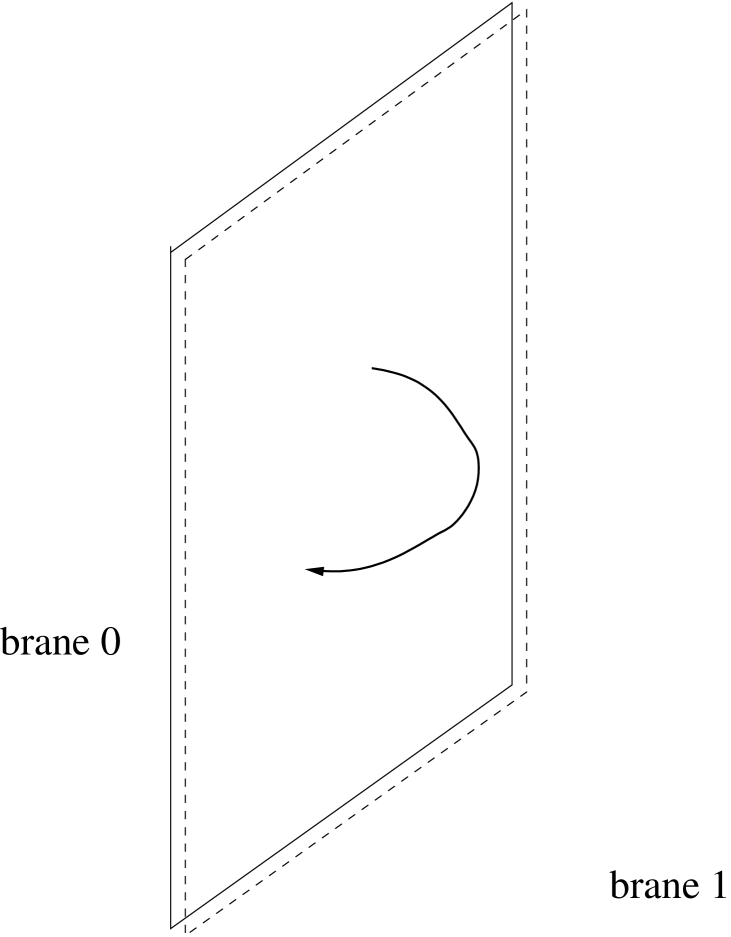
Figure 2: When the branes are coincident one must introduce Chan-Paton since we cannot anymore label the branes by their position.

In our case where the branes are in a generic position the role of the two labels can be taken by $y_{0}$ for the start brane and $y_{\pi}=y_{0}+2\pi(w+\theta)R^{\prime}$ for the end brane. In computing amplitudes we have now to take care that the end brane of a string is the start brane of the next one since this is not anymore implied by matrix multiplication. The effect of momentum (actually width) conservation in DD directions in this formalism is to ensure that the sum of all string widths, defined each as $y_{\pi}-y_{0}$, is zero: this is actually not a new constraint but a consistency condition.

In the limit where some branes are superimposed, the brane position is not anymore enough to distinguish among them and it must be supplemented with a label, thus recovering Chan-Paton factors.

It is interesting to note that amplitude (2.8) is well defined even when there are some non compact directions with DD boundary conditions. When some non compact $X$ have Dirichlet boundary condition it would seem that the correlator in (2.8) be divergent since it is proportional to ${}_{non~{}compact~{}DD}\langle 0|0\rangle_{non~{}compact~{}DD}$ where $|0\rangle_{non~{}compact~{}DD}$ are the would-be momentum vacua in the non compact Dirichlet directions. These vacua $|0\rangle_{non~{}compact~{}DD}$ should naively be normalized as ${}_{non~{}compact~{}DD}\langle 0|0\rangle_{non~{}compact~{}DD}\propto\delta(0)$ since the corresponding directions are non compact but this is not the case. In fact we can normalize ${}_{non~{}compact~{}DD}\langle 0|0\rangle_{non~{}compact~{}DD}=1$ as $|0\rangle_{non~{}compact~{}DD}$ is the only finite energy state because all the “winding states” have energy proportional to $R^{\prime}\rightarrow\infty$. This justifies the point of view that non compact DD directions must be understood as a limit of compactified ones, in particular the spectral decomposition of unity is then given by

$${\hbox{1\kern-3.00003pt1}}_{\mbox{non compact DD}}=\lim_{R^{\prime}\rightarrow\infty}\sum_{w}|\frac{wR^{\prime}}{\alpha^{\prime}}\rangle\langle\frac{wR^{\prime}}{\alpha^{\prime}}|$$ (2.9)

where $|\frac{wR^{\prime}}{\alpha^{\prime}}\rangle$ are the eigenstates of the corresponding $p_{non~{}compact~{}DD}$.

3 The cocycles for vertices.

In this section we first determine the cocycles for closed string vertex operators in closed string formalism so that two closed string vertices commute with each other, then we fix the cocycles for closed string vertex operators in open string formalism by demanding that the normal ordering of the product of two closed string vertices be the same in both closed and open string formalism: this is done in order to be sure that it is possible to describe closed string emission in open formalism at all mass levels and that open/closed string amplitudes are correctly and consistently factorizable in the closed channel. We fix also the cocycles for open string emission vertices so that they commute with closed string ones. In doing so we realize that also $y_{0}$, the quantity entering the left and right moving part of the open string fields given in eq.s (2.2), has to change after the emission of an open string from the $\sigma=0$ border and this change is fundamental even when open string has NN boundary condition (see section 3.3 for an explicit example).

All these cocycles and the transformation of $y_{0}$ turn out to be conceptually very important for a proper amplitudes factorization but of little practical importance as long as one is willing to drop phases in amplitudes.

3.1 The cocycles for the closed string.

As said before the first step is to determine the cocycles in the closed string formalism. A well defined CFT for closed strings must satisfy at least the following criteria

1. closed string vertices commute;

2. a proper behavior under Hermitian conjugation.

The fist request is necessary in order to ensure the mutual locality of closed vertices ([12]), or in other words, that vertices obey the spin-statistics theorem. Usually vertices are written without cocycles as

$${W}^{(c)}_{\beta_{L},\beta_{R}}(z,\bar{z};k) = V_{\beta_{L}}(z;k_{L})\,\,{\tilde{V}}_{\beta_{R}}({\bar{z}};k_{R})$$ (3.10)

where the right moving ${\tilde{V}}_{\beta_{R}}$ is a normal ordered functional of the closed string right moving part

$$X^{(c)\mu}_{R}(\bar{z})=\tilde{q}^{\mu}_{R}-{\rm i}\,{2\alpha^{\prime}}\,\tilde{p}^{\mu}_{R}{}\ln{\bar{z}}+{\rm i}\,\sqrt{2\alpha^{\prime}}\,\sum_{n\not=0}{sgn(n)\over{\sqrt{|n|}}}\tilde{a}_{Rn}^{\mu}{\bar{z}}^{-n}$$ (3.11)

and similarly for the left moving part

$$X^{(c)\mu}_{L}(z)=q^{\mu}_{R}-{\rm i}\,{2\alpha^{\prime}}\,p^{\mu}_{L}{}\ln{z}+{\rm i}\,\sqrt{2\alpha^{\prime}}\,\sum_{n\not=0}{sgn(n)\over{\sqrt{|n|}}}a_{Ln}^{\mu}{z}^{-n}$$ (3.12)

with $z\in{\hbox{l\kern-5.406ptC}}$ and

$$[q_{L}^{\mu},p_{L}^{\nu}]=[q_{R}^{\mu},p_{R}^{\nu}]=i\eta^{\mu\nu}~{}~{}~{}~{}[a_{m}^{\mu},a^{\dagger\nu}_{n}]=[\tilde{a}_{m}^{\mu},\tilde{a}^{\dagger\nu}_{n}]=\delta_{m,n}\eta^{\mu\nu}~{}~{}m,n>0$$ (3.13)

The previous expansions are however not completely exact for the non compact directions since in this case the zero modes are common to left and right moving sectors. Because of this the non compact left and right part of the vertices are not separately normal ordered but only the non zero modes parts are normal ordered separately while the common zero modes are normal ordered together.

For implementing the wanted properties we look for a solution of the form ([12])

$${\cal W}^{(c)}_{\beta_{L},\beta_{R}}(z,\bar{z};k) = c(k_{L},k_{R};p_{L},p_{R})V_{\beta_{L}}(z;k_{L})\,\,{\tilde{V}}_{\beta_{R}}({\bar{z}};k_{R})$$ (3.14)

where the cocycles are given by

$$c(k_{L},k_{R};p_{L},p_{R}) = c_{L}(k_{L},k_{R};p_{L})\,c_{R}(k_{L},k_{R};p_{R})$$ (3.15)

$$= e^{i\pi\alpha^{\prime}({\cal B}k_{L}+{\cal C}k_{R})_{a}\,p_{L}^{a}}\,e^{i\pi\alpha^{\prime}({\cal D}k_{L}+{\cal E}k_{R})_{a}\,p_{R}^{a}}~{}~{}$$

We choose the coefficients ${\cal B},{\cal C},{\cal D},{\cal E}$ to be matrices in order to be general. They have possibly only non vanishing entries in compact directions, e.g ${\cal B}_{a}^{.b}$, since only when there are compact directions they are needed. They must be determined, as said before, so that two arbitrary vertices are mutually local, i.e. commute. This is also equivalent to the fact that the radial ordering of a product of vertices is given by a unique expression which can be derived by analytically continuing whichever particular ordering of the vertices is chosen to perform the computation.

In order to compute these matrices we consider the ordering of the product of two arbitrary vertices as

$${\cal W}^{(c)}_{\beta_{L},\beta_{R}}(z,\bar{z};k_{1}){\cal W}^{(c)}_{\alpha_{L},\alpha_{R}}(w,\bar{w};k_{2}) = e^{i\Phi_{(c)}(k_{1},k_{2})}c(k_{L1}+k_{L2},k_{R1}+k_{R2};p_{L},p_{R})$$

$$\times V_{\beta_{L}}(z;k_{L1})V_{\alpha_{L}}(w;k_{L2})\,\,\,\,{\tilde{V}}_{\beta_{R}}({\bar{z}};k_{R1}){\tilde{V}}_{\alpha_{R}}({\bar{w}};k_{R2})$$

where we have defined the phase

$$\Phi_{(c)}(k_{1},k_{2})=-\pi\,\alpha^{\prime}\left[\left({\cal B}\,k_{L2}+{\cal C}\,k_{R2}\right)\cdot k_{L1}+\left({\cal D}\,k_{L2}+{\cal E}\,k_{R2}\right)\cdot k_{R1}\right]$$ (3.17)

and then we use the well known formula ($-\pi\leq arg(z),arg(w)\leq+\pi$, $|z|<|w|$) (see also appendix B)

$$\left[V(z;k_{1})\,V(w;k_{2})\right]_{\mbox{an.con.}}=V(w;k_{2})\,V(z;k_{1})e^{+i\pi\,sgn(arg(z)-arg(w))\,2\alpha^{\prime}\,k_{1}\cdot k_{2}}$$ (3.18)

to compare with the product of the vertices in the opposite order ${\cal W}^{(c)}_{\alpha_{L},\alpha_{R}}(w,\bar{w};k_{2}){\cal W}^{(c)}_{\beta_{L},\beta_{R}}(z,\bar{z};k_{1})$ and determine the unknown matrices. From the previous equations, as it is described in appendix (C.1), we can deduce that the (matrix) coefficients in compact directions are

$${\cal C}=-{\cal D}=diag(1+2N_{a})\,\,\,\,{\cal B}=-{\cal E}=2~{}diag(M_{a})$$ (3.19)

where $N_{a},M_{a}\in{\mathchoice{\hbox{Z\kern-4.2679ptZ}}{\hbox{Z\kern-4.2679ptZ}}{\hbox{{Z\kern-3.41432ptZ}}}{\hbox{{Z\kern-3.41432ptZ}}}}$. In the rest of the paper we choose

$${\cal C}=-{\cal D}={\hbox{1\kern-3.00003pt1}},~{}~{}~{}~{}{\cal B}=-{\cal E}=0$$ (3.20)

so that the cocycle in eq. (3.15) simply becomes

$$c(k_{L},k_{R};p_{L},p_{R})=e^{i\pi\alpha^{\prime}(k_{Ra}p_{L}^{a}-k_{La}p_{R}^{a})}$$ (3.21)

The action of T-duality on the cocycle of the vertex is not trivial, since it exchanges the possible solutions available, i.e. a T-duality along the compact direction $a$ gives $({\cal C}_{aa},{\cal D}_{aa})\leftrightarrow({\cal D}_{aa},{\cal C}_{aa})$, $({\cal B}_{aa},{\cal E}_{aa})\leftrightarrow({\cal E}_{aa},{\cal B}_{aa})$ or $N_{a}\leftrightarrow-N_{a}-1$, $M_{a}\leftrightarrow-M_{a}$. The question is now whether we have different theories since different choices of cocycles yield amplitudes which differ by a phase. This question assumes that we read the actual effective theory vertices, signs included, from the string amplitudes. At first look we would answer yes since there is no way of redefining the fields of the effective action in a such a way that phases in front of amplitudes match, as it is easy to verify in the case of the three tachyons (see eq. (C.98) in appendix). On the other side also loop corrections are proportional to the same phase of the tree level since moving the cocycles in front of the string of vertices yields the same numeric phase as in the tree level case (this phase depends on external momenta only and does not depend on the number of handles) times an operatorial cocycle like $e^{i\pi\alpha^{\prime}~{}({\cal B}\sum_{j=1}^{N_{c}}k_{Lj}+{\cal C}\sum_{j=1}^{N_{c}}k_{Rj})\cdot p_{L}+\dots}$. Now the above operatorial cocycle is identically $1$ since the numeric coefficients are zero because they are proportional to the sum of the external momenta which are conserved. Because of this the would-be different theories we get give different S-matrix elements which nevertheless yield the same transition probability to all orders in perturbation theory. Moreover the physical states created by the different vertices are the same.

3.2 The cocycles and $y_{0}$ shift in the open string formalism.

A well defined CFT for an open-closed string theory must satisfy at least the following 5 constraints:

1. the open string vertices at $\sigma=0$ and $\sigma=\pi$ commute;

2. the open string emission vertex from $\sigma=0$ commutes with the closed string vertices;

3. in a similar way the open string emission vertex from $\sigma=\pi$ commutes with the closed string vertices;

4. the closed string vertices in open string formalism must have the same “OPE” as in closed string formalism, or more precisely we want the normal ordering of the product of two closed string vertices be formally equal to (3.1), in particular we want the closed string vertices to commute;

5. a proper behavior under Hermitian conjugation.

The previous constraints can fail only because of phases and these phases depend only on momenta therefore the problem amounts to find the proper cocycles and, as we discuss later, the proper shift of the $y_{0}$ (which enters the definition of left and right moving part of the open string expansion given in eq.s (2.2)).

Before writing the vertices it is worth stressing once again what discussed in section 2: we want the closed string vertices be expressed using the open string operators only, i.e. closed strings are made of the same “stuff” of the open string they are emitted. We derive the vertices in appendix C.2, here we limit ourselves to write them explicitly

$${\cal W}_{\beta_{L},\beta_{R}}(z,\bar{z};k_{L},k_{R}) = e^{-i\pi\alpha^{\prime}\,(Sk_{L}\cdot k_{R})}{V}_{\beta_{L}}(X_{L}(z);k_{L}){}~{}{V}_{\beta_{R}}(X_{R}(\bar{z});k_{R})$$

$${\cal V}_{\alpha}(x;k) = {V}_{\alpha}(X_{L}(x){-y_{0}};k)\,~{}~{}~{}~{}x>0$$ (3.23)

along with the vertices for the emission from the $\sigma=\pi$ boundary

$${\cal V}_{\alpha}(x;k) = e^{-2i\pi\,k\cdot p}{V}_{\alpha}(X_{L}(x){-y_{0}};k)\,~{}~{}~{}~{}x<0.$$ (3.24)

In this case the action of the cocycle simply means that we can substitute $\left[X_{L}(x)-y_{0}\right]_{zero~{}mode}=q-2\alpha^{\prime}ip\log(x)\rightarrow q-2\alpha^{\prime}ip\log(|x|)$ and drop the cocycle.

While the previous vertices seem essentially the normal vertices, the closed string vertex does depend on $y_{0}$ since

$${\cal W}_{\beta_{L},\beta_{R}}(z,\bar{z};k_{L},k_{R})\sim e^{iy_{0}\cdot(k_{L}-Sk_{R})}\dots$$ (3.25)

and $y_{0}$ changes along the worldsheet. This happens because we are taking the original point of view of [9] according to which the “stuff” of the “carrier” string may change after the emission of another open string. Because of this the closed string emission vertices do not change in form when written using the “carrier” string fields from which the closed string states are emitted but they do change when the actual “carrier” string fields are expressed using the fields of incoming “carrier” string.

The change of $y_{0}$ can be better appreciated by considering a carrier open string with Dirichlet b.c. in at least one compact direction. In fig.s 3 we have pictured in two ways the interaction between an incoming open string stretched between brane 0 and brane 1 with another open string, the emitted string, stretched between brane 2 and brane 0. The incoming string has DD b.c. $X^{in}(\sigma=0)=y_{0}$ and $X^{in}(\sigma=\pi)=y_{0}+\delta^{in}$ with $\delta^{in}=2\pi\alpha^{\prime}k_{in}$. The other string, which is emitted from the incoming one, stretches between $X^{emitted}(\sigma=0)=y_{0}^{emitted}=y_{0}-\delta^{emitted}$ and $X^{emitted}(\sigma=\pi)=y_{0}^{emitted}+\delta^{emitted}=y_{0}$. The result of the interaction is the outgoing string with $X^{out}(\sigma=0)=y_{0}^{out}=y_{0}^{emitted}=y_{0}-\delta^{emitted}$ and $X^{out}(\sigma=\pi)=y_{0}^{out}+\delta^{out}=y_{0}+\delta^{in}+\delta^{emitted}$. The latter equation has a simple interpretation: when a string with DD b.c. is emitted from the $\sigma=0$ border of the incoming open string the outgoing string has width equal to the sum of the incoming carrier string $\delta_{in}$ and the emitted string $\delta_{emitted}$. This is taken care by the momentum $p$ conservation but the position of the $\sigma=0$ border of the outgoing string is changed in such a way the position of the $\sigma=\pi$ border is left unchanged, i.e.

$$y_{0}^{out}=y_{0}-\delta_{emitted}~{}~{}~{}\delta_{emitted}=2\pi\alpha^{\prime}k_{emitted}.$$ (3.26)

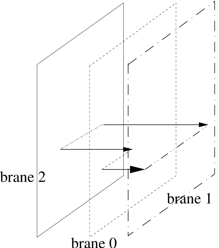
Figure 3: Two different pictures of the emission of a string from an incoming one which transforms into an outgoing string. The incoming string stretches between brane 0 at $y_{0}^{in}$ and brane 1 at $y_{0}^{in}+\delta_{in}$ ($\delta_{in}=2\pi\alpha^{\prime}k_{in}$); the emitted string stretches between brane 2 at $y_{0}^{out}$ and brane 0 at $y_{0}^{out}+\delta_{emitted}=y_{0}^{in}$ ($\delta_{emitted}=2\pi\alpha^{\prime}k_{emitted}$) and the outgoing string between brane 2 at $y_{0}^{out}=y_{0}^{in}-\delta_{emitted}$ and brane 1 at $y_{0}^{out}+\delta_{emitted}+\delta_{in}$.

The main point hence is that the open string changes its b.c. after the emission of a string from the $\sigma=0$ boundary and therefore $y_{0}$ changes too accordingly. Hence the closed string vertex does change when expressed using the incoming string fields.

Because of the expansions in eq.s (2.2) this change in $y_{0}$ means

$$X^{out}_{L}=X^{in}_{L}-\delta_{emitted}$$ (3.27)

and

$$X^{out}_{R}=X^{in}_{R}+S\delta_{emitted}$$ (3.28)

Hence the closed string vertex changes when inserted before or after the emission of the open string from the $\sigma=0$ boundary. The proper commutation relation between a closed string and an open string emitted from $\sigma=0$ then reads

$$\left[{\cal W}_{\beta_{L},\beta_{R}}(X_{L}^{out}(z),X_{R}^{out}(\bar{z}))\,{\cal V}_{\alpha}(x;k)\right]_{an.con.} = {\cal V}_{\alpha}(x;k)\,{\cal W}_{\beta_{L},\beta_{R}}(X_{L}^{in}(z),X_{R}^{in}(\bar{z}))$$

$$= {\cal V}_{\alpha}(x;k)\,{\cal W}_{\beta_{L},\beta_{R}}(X_{L}^{out}(z),X_{R}^{out}(\bar{z}))e^{2\pi\alpha^{\prime}i\,k\cdot(k_{L}-Sk_{R})}$$

$$= \left[{\cal W}_{\beta_{L},\beta_{R}}(X_{L}^{in}(z),X_{R}^{in}(\bar{z}))\,{\cal V}_{\alpha}(x;k)\right]_{an.con.}e^{-2\pi\alpha^{\prime}i\,k\cdot(k_{L}-Sk_{R})}$$

where we have used the fact that $\delta=2\pi\alpha^{\prime}k$ and $an.con.$ means analytically continued.

3.3 An explicit example.

The importance of the cocycle factors and the $y_{0}$ shift for a full consistency of amplitudes and the proper understanding of the consequences of commutation relation eq. (LABEL:W_V_commutation) can be appreciated computing in the operatorial formalism the one closed tachyon - one open tachyon amplitude in two different ways either

$$\langle 0|{\cal W}_{T}(k_{L},k_{R};z,\bar{z})\,{\cal V}_{T}(k;x)|0\rangle~{}~{}~{}~{}~{}~{}|z|>|x|$$ (3.30)

or

$$\langle 0|{\cal V}_{T}(k;x)\,{\cal W}_{T}(k_{L},k_{R};z,\bar{z})|0\rangle~{}~{}~{}~{}~{}~{}|x|>|z|.$$ (3.31)

In the second way we find

$$~{}\langle 0|{\cal V}_{T}(k;x)\,{\cal W}_{T}(k_{L},k_{R};z,\bar{z})|0\rangle~{}~{}~{}~{}~{}~{}|x|>|z|$$ (3.32)

$$\langle 0|:e^{ik\cdot(X_{L}(x)-y_{0})}:~{}:e^{ik_{L}\cdot X_{L}(z)}:\,:e^{ik_{R}\cdot X_{R}(\bar{z})}:|0\rangle$$

$$= e^{i(k_{L}-Sk_{R})\cdot y_{0}}|z-\bar{z}|^{2\alpha^{\prime}k_{L}\cdot Sk_{R}}(x-z)^{2\alpha^{\prime}k\cdot k_{L}}(x-\bar{z})^{2\alpha^{\prime}k\cdot k_{R}}$$

$$(2\pi)^{D_{NN,nc}}\delta^{D_{NN,nc}}(k+k_{L}+k_{R})\delta^{D_{NN,c}+D_{DD}}_{k+k_{L}+Sk_{R},0}$$

$$= e^{i(k_{L}-Sk_{R})\cdot y_{0}}|z-\bar{z}|^{2\alpha^{\prime}k_{L}\cdot Sk_{R}}|x-z|^{2\alpha^{\prime}k\cdot(k_{L}+Sk_{R})}$$

$$\left(\frac{x-z}{x-\bar{z}}\right)^{\alpha^{\prime}k\cdot(k_{L}-Sk_{R})}(2\pi)^{D_{NN,nc}}\delta^{D_{NN,nc}}(k+k_{L}+k_{R})\delta^{D_{NN,c}+D_{DD}}_{k+k_{L}+Sk_{R},0}$$

$$= e^{i(k_{L}-Sk_{R})\cdot y_{0}}|z-\bar{z}|^{-1}|x-z|^{-2}\left(2\pi\delta(k+k_{L}+k_{R})\right)^{D_{NN,nc}}\delta^{D_{NN,c}+D_{DD}}_{k+k_{L}+Sk_{R},0}$$

where $D_{DD}$ is the number of directions with DD boundary condition, $D_{NN,c}$ ($D_{NN,nc}$) is the number of compact (non compact) directions with NN boundary condition and we have written the modulus $|z-\bar{z}|^{\cdots}$ and not $(z-\bar{z})^{...}$ because of the contribution from the cocycle $e^{-i\pi\alpha^{\prime}\,(Sk_{L}\cdot k_{R})}$ of closed string vertex cocycle. The last line is obtained using the momentum conservation and mass shell conditions $k_{L}^{2}=k_{R}^{2}=k^{2}=\frac{1}{\alpha^{\prime}}$ and shows how the amplitude is conformal invariant when ghost contribution is added.

Let us now consider the computation for $|z|>x$. According to our previous discussion it requires the use of the closed string emission vertex depending on $X_{out}$

$${\cal W}_{T}(k_{L},k_{R};z,\bar{z}) = e^{-i\pi\alpha^{\prime}Sk_{L}\cdot k_{R}}~{}:e^{ik_{L}\cdot X_{L}^{out}(z)}:\,:e^{ik_{R}\cdot X_{R}^{out}(\bar{z})}:$$

$$= e^{-i\pi\alpha^{\prime}Sk_{L}\cdot k_{R}}~{}:e^{ik_{L}\cdot(X_{L}(z)-2\pi\alpha^{\prime}k)}:\,:e^{ik_{R}\cdot(X_{R}(\bar{z})+2\pi\alpha^{\prime}Sk)}:$$

The shift of $y_{0}$ by $2\pi\alpha^{\prime}k$ is necessary in computing this correlator, in fact

$$~{}\langle 0|{\cal W}_{T}(k_{L},k_{R};z,\bar{z})\,{\cal V}_{T}(k;x)0|\rangle~{}~{}~{}~{}~{}~{}|z|>|x|$$

$$= \langle 0|:e^{ik_{L}\cdot X_{L}^{out}(z)}:\,:e^{ik_{R}\cdot X_{R}^{out}(\bar{z})}::e^{ik\cdot(X_{L}(x)-y_{0})}:~{}|0\rangle$$

$$= e^{-i2\pi\alpha^{\prime}k\cdot(k_{L}-Sk_{R})}e^{i(k_{L}-Sk_{R})\cdot y_{0}}|z-\bar{z}|^{2\alpha^{\prime}k_{L}\cdot Sk_{R}}(z-x)^{2\alpha^{\prime}k\cdot k_{L}}(\bar{z}-x)^{2\alpha^{\prime}k\cdot k_{R}}$$

$$(2\pi)^{D_{NN,nc}}\delta^{D_{NN,nc}}(k+k_{L}+k_{R})\delta^{D_{NN,c}+D_{DD}}_{k+k_{L}+Sk_{R},0}$$

$$= e^{i(k_{L}-Sk_{R})\cdot y_{0}}|z-\bar{z}|^{2\alpha^{\prime}k_{L}\cdot Sk_{R}}|z-x|^{2\alpha^{\prime}k\cdot(k_{L}+Sk_{R})}$$

$$e^{-i2\pi\alpha^{\prime}k\cdot(k_{L}-Sk_{R})}\left(\frac{z-x}{\bar{z}-x}\right)^{\alpha^{\prime}k\cdot(k_{L}-Sk_{R})}(2\pi)^{D_{NN,nc}}\delta^{D_{NN,nc}}(k+k_{L}+k_{R})\delta^{D_{NN,c}+D_{DD}}_{k+k_{L}+Sk_{R},0}$$

$$= e^{i(k_{L}-Sk_{R})\cdot y_{0}}|z-\bar{z}|^{2\alpha^{\prime}k_{L}\cdot Sk_{R}}|x-z|^{2\alpha^{\prime}k\cdot(k_{L}+Sk_{R})}$$

$$\left(\frac{x-z}{x-\bar{z}}\right)^{\alpha^{\prime}k\cdot(k_{L}-Sk_{R})}(2\pi)^{D_{NN,nc}}\delta^{D_{NN,nc}}(k+k_{L}+k_{R})\delta^{D_{NN,c}+D_{DD}}_{k+k_{L}+Sk_{R},0}$$

where the phase from the shift $e^{-i2\pi\alpha^{\prime}k\cdot(k_{L}-Sk_{R})}$ is necessary to compensate the phase obtained analytically continuing (also off shell where $k\cdot(k_{L}-Sk_{R})\neq-(k_{L}+Sk_{R})\cdot(k_{L}-Sk_{R})$ ) $\left(\frac{z-x}{\bar{z}-x}\right)^{\alpha^{\prime}k\cdot(k_{L}-Sk_{R})}$ to the region $x>|z|$. In performing this analytical continuation one has to use

$$\left[\log(z-w)\right]_{an.~{}cont.}=\log(w-z)+i\pi~{}sign(arg(z)-arg(w))~{}~{}~{}~{}-\pi<arg(z),arg(w)<\pi$$ (3.34)

which in this case gives $\left[\log(z-x)\right]_{an.~{}cont.}=\log(x-z)+i\pi$ and its complex conjugate expression $\left[\log(\bar{z}-x)\right]_{an.~{}cont.}=\log(x-\bar{z})-i\pi$.

4 Amplitudes factorization.

Since we are trying to ensure that all intermediate expressions be well defined with respect to vertices commutativity property and to keep track of how and where phases arise, the naive procedure adopted in ([9],[13]) is not completely valid: details on how this can be accomplished are given in app. D, here we give only the main steps.

We start considering the correlator (which is denoted by a capital $A$ and is not the amplitude which needs an integration over the moduli space which we consider later )

$$A(N_{o},N_{c})=\prod_{i=1}^{N_{o}-1}\theta(|x_{i+1}|-|x_{i}|)\,\langle 0|~{}{\rm T}\left(\prod_{i=1}^{N_{o}}{\cal V}_{\alpha_{i}}(x_{i};k_{i})dx_{i}\,\prod_{j=1}^{N_{c}}{\cal W}_{\beta_{Lj},\beta_{Rj}}(z_{j},\bar{z}_{j};k_{L/R~{}j})d^{2}z_{j}\right)|0\rangle~{}~{}$$ (4.35)

where the $x$s are real (both positive and negative), all $z$s are in the upper half-plane $\,\,{\hbox{l\kern-5.406ptH}}^{+}$, the vacuum state $|0\rangle$ is defined as $|0\rangle=\prod_{\mu=1}^{\mu=D}|p_{\mu}=0;0_{a}\rangle$ and it is normalized as

$$\langle p_{\mu}=0|p_{\mu}=0\rangle=\left\{\begin{array}[]{cc}\mbox{non compact NN}&2\pi\delta(0)\\ \mbox{non compact DD}&1\\ \mbox{compact}&1\end{array}\right.$$ (4.36)

The normalization of the non compact directions with Dirichlet boundary condition may seem strange but one has to keep in mind that in this case only $|0\rangle_{\mbox{non compact DD}}$ has finite energy since the “momentum” spectrum is $\frac{wR}{\alpha^{\prime}}$; nevertheless the spectral decomposition of unity is still given by

$${\hbox{1\kern-3.00003pt1}}_{\mbox{non compact DD}}=\lim_{R\rightarrow\infty}\sum_{w}|\frac{wR}{\alpha^{\prime}}\rangle\langle\frac{wR}{\alpha^{\prime}}|$$ (4.37)

and because of this the non compact DD case must be understood as a special decompactification limit: using the naive result would lead to a wrong result.

On this correlator we want to perform the $SL(2,{\hbox{l\kern-5.406ptC}})$ transformation

$$w={z+{\rm i}\over z-{\rm i}}~{}~{}~{}$$ (4.38)

which maps $x\in{\hbox{l\kern-1.42262ptR}}\rightarrow w(x)=e^{i\phi}$, $z\in{\hbox{l\kern-5.406ptH}}^{+}\rightarrow w(z)$ with $|w(z)|>1$ and $\bar{z}\rightarrow w(\bar{z})=(\overline{w(z)})^{-1}$ by inserting the corresponding $SL(2,{\hbox{l\kern-5.406ptC}})$ operator. In this way we move form the graphical representation given in fig. (5) to the one in fig. (5).

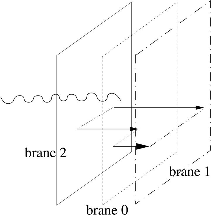
Figure 4: A 3 parallel branes interaction with 3 open strings and 1 closed one.

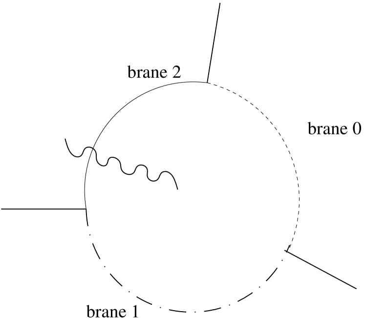
Figure 5: The same configuration as the previous picture with the usual disk picture. This representation is obtained after changing variables as in eq. (4.38).

The final answer is given by the following correlator as discussed in appendix D

$$A(N_{o},N_{c}) = e^{i\alpha_{0}}\langle 0|~{}{\rm T}\Big{(}\prod_{i=1}^{N_{o}}{V}_{\alpha_{i}}(e^{i\phi_{i}};k_{i})de^{i\phi_{i}}\,\prod_{l=1}^{N_{o}-1}\theta(\phi_{l}-\phi_{l+1})$$ (4.39)

$$\,\prod_{j=1}^{N_{o}}c_{L}(k_{Lj},k_{Rj};p)\,e^{ik_{Lj}y_{0}}{V}_{\beta_{Lj}}(w_{j};k_{Lj})dw_{j}$$

$$\,\prod_{l=1}^{N_{c}}c_{R}(k_{Ll},k_{Rl};-Sp)\,e^{-iSk_{Rj}y_{0}}{V}_{\beta_{Rl}}(\frac{1}{\bar{w}_{l}};k_{Rl})\frac{d\bar{w}_{l}}{\bar{w}^{2}_{l}}\Big{)}|0\rangle~{}~{}$$

where we have made explicit the $y_{0}$ dependence by redefining the $X_{L,R}$ in such a way they are free of $y_{0}$ and we have introduced the cocycles $c_{L}$ and $c_{R}$ to ensure that the amplitude can be obtained by the analytic continuation of whichever radial order. It is important to stress that thanks to the cocycle the phase $\alpha_{0}$ is independent of the different specific cases which arise from the radial ordering.

4.1 Spectral decomposition of the unity in the disk channel.

We can now proceed as in ([9],[13]) and we insert a complete set of states at radial time $1^{-}$. Since we are in the open string channel there is only one momentum flowing for each direction and therefore we want to insert something like ${\hbox{1\kern-3.00003pt1}}=\int_{q}|q\rangle\langle q|$ as far as the zero modes are concerned. The naive guess is that we can insert the usual open string version of the spectral decomposition of unity

$${\hbox{1\kern-3.00003pt1}}_{naive}=\sum_{\lambda,q,n,w}|\lambda,(q,\frac{n}{R},\frac{wR}{\alpha^{\prime}})\rangle\langle\lambda,(q,\frac{n}{R},\frac{wR}{\alpha^{\prime}})|$$ (4.40)

with continuous momentum $q$ flowing in non compact NN directions, momentum $\frac{n}{R}$ flowing in compact NN directions and winding $\frac{wR}{\alpha^{\prime}}$ flowing in compact DD ones, unfortunately this guess is wrong. To understand what is going on we analyze what flows in compact directions. The momentum conservation reads

$$\sum_{j=1}^{N_{c}}(k_{Lj}+Sk_{Rj})+\sum_{i=1}^{N_{o}}k_{i}=0$$ (4.41)

(with $S=+1$ in NN directions and $S=-1$ in DD directions) and because we are inserting 11 at radial time $1^{-}$ this equation can be split into two different relations

$$\left\{\begin{array}[]{cc}\sum_{j=1}^{N_{c}}Sk_{Rj}+q=0&\frac{1}{|w|}<1^{-}\\ -q+\sum_{j=1}^{N_{c}}k_{Lj}+\sum_{i=1}^{N_{o}}k_{i}=0&|e^{i\phi}|,|w|>1^{-}\end{array}\right.$$ (4.42)

In compact NN directions the second equation can be written in a more explicit way as

$$\frac{1}{R}(\frac{1}{2}\sum_{j=1}^{N_{c}}n_{j}+\sum_{i=1}^{N_{o}}(n_{i}+\theta_{i}))+\frac{R}{2\alpha^{\prime}}\sum_{j=1}^{N_{c}}w_{j}-q=0$$ (4.43)

(and in compact DD direction as

$$\frac{1}{2R}\sum_{j=1}^{N_{c}}n_{j}+\frac{R}{\alpha^{\prime}}(\frac{1}{2}\sum_{j=1}^{N_{c}}w_{j}+\sum_{i=1}^{N_{o}}(w_{i}+\theta_{i}))-q=0$$ (4.44)

). Since winding $w$ (momentum $n$) of the closed string states must be unrestricted in NN (DD) directions a first guess would be to sum over $q=\frac{Rw}{2\alpha^{\prime}}$ $\forall w\in{\mathchoice{\hbox{Z\kern-4.2679ptZ}}{\hbox{Z\kern-4.2679ptZ}}{\hbox{{Z\kern-3.41432ptZ}}}{\hbox{{Z\kern-3.41432ptZ}}}}$ ($q=\frac{n}{2R}$ $\forall n\in{\mathchoice{\hbox{Z\kern-4.2679ptZ}}{\hbox{Z\kern-4.2679ptZ}}{\hbox{{Z\kern-3.41432ptZ}}}{\hbox{{Z\kern-3.41432ptZ}}}}$) but this is not yet completely right. Choosing these values for $q$ eq. (4.43) for the NN directions becomes

$$\frac{1}{2}\sum_{j=1}^{N_{c}}n_{j}+\sum_{i=1}^{N_{o}}(n_{i}+\theta_{i})=0$$ (4.45)

and because of the factor $\frac{1}{2}$ which multiplies $\sum_{j=1}^{N_{c}}n_{j}$ in this equation, we get a wrong momentum conservation (and similarly for DD directions). On the other hand summing over all $q=\frac{1}{2}\left(\frac{n}{R}+\frac{wR}{\alpha^{\prime}}\right)$ (both $n$ and $w$) would give a wrong one loop amplitude. The right answer for generic $R$s, even if strange, is the following (closed string like) spectral decomposition of unity

11 $$= \sum_{\lambda,q,w,n}|\lambda,\{q,w,n\}\rangle\langle\lambda,\{q,w,n\}|$$

$$= \sum_{\lambda,q,w,n}|\lambda,(q,-\frac{\sum_{i=1}^{N_{o}}k_{i}}{2}+\frac{wR}{2\alpha^{\prime}},-\frac{\sum_{i=1}^{N_{o}}k_{i}}{2}+\frac{n}{2R})\rangle\langle\lambda,(q,-\frac{\sum_{i=1}^{N_{o}}k_{i}}{2}+\frac{wR}{2\alpha^{\prime}},-\frac{\sum_{i=1}^{N_{o}}k_{i}}{2}+\frac{n}{2R})|$$

(4.46)

where we have a sum of shifted winding for any NN compact direction and sum of shifted momentum for any DD compact direction. In non compact directions $\sum_{q}$ has to be understood as the result of decompactification limit, i.e. $\int\frac{dq}{2\pi}$ for any non compact DD direction and $\lim_{R\rightarrow\infty}\sum_{w}|\frac{wR}{\alpha^{\prime}}\rangle\langle\frac{wR}{\alpha^{\prime}}|$ for any non compact NN direction. This result is a clue that already at tree level open string knows of the existence of closed string. On the other side one could argue that is not completely surprising since we are computing a mixed open-closed amplitude, even so we can understand better why this happens by noticing that this spectral decomposition of unity is not what one naively would expect because, while factorizing, we are separating the left and right part of closed string vertex operators.

4.2 Factorizing the disk amplitude.

Inserting the unity given in eq (4.1) into eq. (4.39) we get

$$A(N_{o},N_{c}) = e^{i\alpha_{0}}e^{iy_{0}\left(\sum_{j=1}^{N_{c}}(k_{Lj}-Sk_{Rj}){}\right)}\prod\theta(\phi_{i}-\phi_{i+1})$$

$$\sum_{\lambda,q,w,n}\langle 0|T\left(\,\prod_{j=1}^{N_{c}}c_{L}(k_{Lj},k_{Rj};p)\,{V}_{\beta_{Lj}}(w_{j};k_{Lj})dw_{j}\right)$$

$$\prod_{i=1}^{N_{o}}{\cal V}_{\alpha_{i}}(e^{i\phi_{i}};k_{i})de^{i\phi_{i}}|\lambda,\{q,w,n\}\rangle$$

$$\langle\lambda,\{q,w,n\}|T\left(\,\prod_{l=1}^{N_{c}}c_{R}(k_{Ll},k_{Rl};-Sp)\,{V}_{\beta_{Rl}}(\frac{1}{\bar{w}_{l}};k_{Rl})\frac{d\bar{w}_{l}}{\bar{w}^{2}_{l}}\right)|0\rangle~{}~{}$$

(4.47)

We can then take the transpose of the piece containing $V_{\beta_{R}}$s and get

$$A(N_{o},N_{c}) = e^{i\alpha_{1}}e^{iy_{0}\left(\sum_{j=1}^{N_{c}}(k_{Lj}-Sk_{Rj}){}\right)}\prod\theta(\phi_{i}-\phi_{i+1})$$

$$\sum_{\lambda,q,w,n}\langle 0|T\Big{(}\,\prod_{j=1}^{N_{c}}c_{L}(k_{Lj},k_{Rj};p)\,{V}_{\beta_{Lj}}(w_{j};k_{Lj})dw_{j}\Big{)}$$

$$\prod_{i=1}^{N_{o}}{\cal V}_{\alpha_{i}}(e^{i\phi_{i}};k_{i})de^{i\phi_{i}}|\lambda,\{q,w,n\}\rangle$$

$$\langle 0|T\Big{(}\,\prod_{l=1}^{N_{c}}c_{R}(k_{Ll},k_{Rl};Sp)\,{V}_{\beta_{Rl}}({\bar{w}_{l}};k_{Rl}){d\bar{w}_{l}}\Big{)}|\lambda,\{-q,-w,-n\}\rangle~{}~{}$$

(4.48)

where in the last line we have used the transposition rule

$$\left[c_{R}(k_{L},k_{R};-Sp)\,{V}_{\beta_{R}}(\frac{1}{\bar{w}};k_{R})\right]^{T}=V_{\beta_{R}}({\bar{w}};k_{R})c_{R}(k_{L},k_{R};Sp){\bar{w}}^{2}$$ (4.49)

and we have changed the overall phase $\alpha_{0}\rightarrow\alpha_{1}$ due to the reordering of cocycles.

Now the last line is invariant under the substitution

$$(k_{R},X_{R}\equiv SX_{R}^{(NN)},\lambda,q,w,n)\rightarrow(k_{R},X_{R}^{(NN)}({\bar{w}}),S\lambda,Sq,Sw,Sn),$$ (4.50)

so we can perform this substitution and then the renaming

$$(X_{L},X_{R}^{(NN)},\lambda,q,w,n)\rightarrow(X_{L}^{(c)},\tilde{X}_{R}^{(c)},\tilde{\lambda},\tilde{q},\tilde{w},\tilde{n})$$ (4.51)

Finally we can rewrite eq. (4.2) as follows

$$A(N_{o},N_{c}) =e^{i\alpha_{1}}\langle\tilde{0}|\langle 0|T\Big{(}\,\prod_{j=1}^{N_{c}}c_{L}(k_{j};p)\,c_{R}(k_{j};\tilde{p})\,{V}_{\beta_{Lj}}(w_{j};k_{Lj}){\tilde{V}}_{\beta_{Lj}}(\bar{w}_{j};k_{Rj})d^{2}w_{j}\Big{)}$$

$$\prod_{i=1}^{N_{o}}\theta(\phi_{i}-\phi_{i+1}){\cal V}_{\alpha_{i}}(e^{i\phi_{i}};k_{i})de^{i\phi_{i}}$$

$$\sum_{\lambda,q,w,n}e^{iy_{0}\left(\sum_{j=1}^{N_{c}}(k_{Lj}-Sk_{Rj}){}\right)}|\lambda,\{q,w,n\}\rangle|S\tilde{\lambda},\{-S\tilde{q},-S\tilde{w},-S{\tilde{n}}\}\rangle$$

(4.52)

This expression involves two different sets of operators, like $a$ and $\tilde{a}$ which can be interpreted as the left and right moving operators of a closed string; because of this interpretation ${\cal V}_{\alpha}$ is now expressed using left moving closed string $X_{L}^{(c)}(z)$ only.

As it is evident from eq. (4.2) this open string derived formalism treats in a uniform way compact and non compact directions, this is not what happens in closed string formalism where zero modes sectors differ in compact and non compact directions. It is however not difficult to see that the two formalisms actually yield the same answer in zero modes sector only when the NN case is treated as a decompactification limit as stated before.

4.3 The boundary state.

In order to derive our final expression for the boundary state we must now take care of the last three ingredients entering the complete amplitude given in eq. (2.8) which were left out in computing the correlator in eq. (4.35): the normalization factors, the integration region and the projective volume. The latter is very easily taken care of by fixing a closed string emission vertex at $z_{1}=ie^{\epsilon}\rightarrow w_{1}=\infty$ ($\epsilon\rightarrow 0$) and an open one at $x_{N_{o}}=+\infty\rightarrow\phi_{N_{o}}=0$, this means that in this limit the conformal group volume can be written as

$$dV_{abc} = \frac{d^{2}z_{1}\,dx_{N_{o}}}{i(z_{1}-\bar{z}_{1})(x_{N_{o}}-z_{1})(x_{N_{o}}-\bar{z}_{1})}=\frac{d^{2}w_{1}\,d(e^{i\phi_{N_{o}}})}{i(|w_{1}|^{2}-1)(w_{1}-e^{i\phi_{N_{o}}})(e^{i\phi_{N_{o}}}\bar{w}_{1}-1)}$$ (4.53)

$$\longrightarrow_{w_{1}\rightarrow\infty} \frac{d^{2}w_{1}\,d(e^{i\phi_{N_{o}}})}{ie^{i\phi_{N_{o}}}|w_{1}|^{4}};$$

since the amplitude must be invariant under the gauge fixing it follows that the correlator (when integrated over the remaining variables) is $A(N_{0},N_{c})\propto e^{-i\phi_{N_{o}}}$ and hence we can decide to only fix the closed string vertex at $z_{1}=ie^{\epsilon}$ and let the open string vertex be free if we integrate the so partially gauge fixed amplitude over $\int_{0}^{2\pi}\frac{de^{i\phi_{N_{o}}}}{2\pi}$ and, at the same time, we transform the $\theta(\phi_{i}-\phi_{i+1})$ into a periodic $\theta_{P}(\phi_{i}-\phi_{i+1})$ to ensure only the proper sequence of the vertices.

The normalization in eq. (2.8) left out in eq. (4.35) is ${\cal C}_{0(p)}\,{\cal N}_{o(p)}^{N_{o}}\,{{\cal N}_{c}}^{N_{c}}$. Since we want to interpret eq. (4.2) as a closed string amplitude it should be normalized as ${\cal N}_{c}^{N_{c}-1}$ since the boundary state is not a normal closed string state, were it a normal state we would normalize the amplitude as ${\cal\widehat{C}}_{0}{\cal N}_{c}^{N_{c}}$ where ${\cal\widehat{C}}_{0}$ is the closed string sphere normalization but this is not the proper recipe to obtain the one point closed string emission from the boundary state which reads $\langle\phi|B\rangle$ where $|\phi\rangle$ is a generic closed string state . It then follows that the boundary state must be multiplied by ${\cal C}_{0(p)}{\cal N}_{o(p)}^{N_{o}}{\cal N}_{c}=\frac{T_{p}}{2}{\cal N}_{o(p)}^{N_{o}}$. From this expression it is clear that the insertion of $N_{o}$ open string states implies, as expected, only a multiplicative factor ${\cal N}_{o}^{N_{o}}$ with respect to the “bare” boundary state.

Finally remembering the shift of the compact momenta in the partition of unity given in eq. (4.1) we can write the boundary state describing multiple parallel interacting $Dp$ branes in generic position as

$$|Dp,\{k_{i},\alpha_{i}\}_{\{1\leq i\leq N_{o}\}}\rangle = e^{i\alpha(p)}\Bigg{[}{\cal N}_{o(p)}^{N_{o}}\prod_{i=1}^{N_{o}}\int_{0}^{2\pi}\theta_{P}(\phi_{i}-\phi_{i+1})de^{i\phi_{i}}{\cal V}_{\alpha_{i}}(X^{(c)}_{L}(e^{i\phi_{i}});k_{i})\Bigg{]}$$ (4.54)

$$\times e^{-i\sum_{i=1}^{N_{o}}k_{i}\cdot\left(\frac{x_{L}-Sx_{R}}{2}{}\right)}|Dp\rangle$$

$$= e^{i\alpha(p)}\Bigg{[}2\pi i{\cal N}_{o(p)}^{N_{o}}\prod_{i=1}^{N_{o}-1}\int_{0}^{2\pi}\theta(\phi_{i}-\phi_{i+1})de^{i\phi_{i}}{\cal V}_{\alpha_{i}}(X^{(c)}_{L}(e^{i\phi_{i}});k_{i})\Bigg{]}$$

$$\times e^{-i\sum_{i=1}^{N_{o}}k_{i}\cdot\left(\frac{x_{L}-Sx_{R}}{2}{}\right)}|Dp\rangle~{}$$

where the open string vertices ${\cal V}_{\alpha_{i}}(X^{(c)}_{L}(e^{i\phi_{i}});k_{i})$ are functionally the same open string vertex operators as in eq. (3.23) but now they functionally depend not on the open string fields but on the left moving part of the closed string fields $X^{(c)}$: to stress this we have explicitly added $(c)$ to the notation.

The operatorial phase is given by

$$e^{i\alpha(p)}=e^{-i\pi\alpha^{\prime}p_{L}\cdot Sp_{R}}$$ (4.55)

with $p_{L}=p_{R}$ in non compact direction as shown in appendix (D.1).

In the first line of eq. (4.54) we have introduced a further angle $\phi_{N_{o}+1}=\phi_{1}$ because we have used a periodic $\theta_{P}$ and we integrate over all the $N_{o}$ positions while in the second we have set $\phi_{N_{o}}=0$, used a normal $\theta$ and we integrate over the first $N_{o}-1$ positions. We have also introduced the usual boundary state

$$|Dp\rangle = {\cal C}_{0(p)}{1\over 2\pi}\sum_{\lambda,q,w,n}e^{-2iy_{0}\cdot(q,\frac{wR}{2\alpha^{\prime}},\frac{n}{R})}|\lambda,(q,\frac{wR}{2\alpha^{\prime}},\frac{n}{R})\rangle|S\tilde{\lambda},(-S\tilde{q},-S\frac{\tilde{w}R}{2\alpha^{\prime}},-S\frac{\tilde{n}}{R})\rangle$$ (4.56)

$$= \frac{T_{p}}{2}e^{-\sum_{n=1}^{\infty}a^{\dagger}_{n}\cdot S\cdot\tilde{a}^{\dagger}_{n}}|Dp_{0}\rangle$$

with the zero modes part

$$|Dp_{0}\rangle = \delta^{{\hat{d}}-p_{nc}-1}(x-y_{0})|p_{\alpha}=0>\sum_{w}e^{i\frac{wR}{\alpha^{\prime}}\left(\frac{x_{L}-x_{R}}{2}-y_{0}\right)}|0,\tilde{0}\rangle_{NN}\sum_{n}e^{i\frac{n}{R}\left(\frac{x_{L}+x_{R}}{2}-y_{0}\right)}|0,\tilde{0}\rangle_{DD}$$

(4.57)

To derive this result we have explicitly used the momentum conservation and $S_{DD}=-1$ and $S_{NN}=+1$ , moreover we have added $DD$ and $NN$ to remember from which open string boundary condition the pieces were originated and we have supposed to have $p_{nc}=D_{NN,nc}-1=D-1-D_{DD}-D_{NN,c}$ non compact spacial directions along the brane and we have defined the brane tension $\frac{T_{p}}{2}=\frac{{\cal C}_{0(p)}{\cal N}_{c}}{2\pi}$. The meaning of the insertion of $exp(-i\sum_{i=1}^{N_{o}}k_{i}\frac{x_{L}-Sx_{R}}{2})$ in eq. (4.54) (which gives a non vanishing contribution for compact directions only) is to divide in the proper way the open string momentum in the left and right moving momentum in order to ensure that the closed string momentum emitted from the boundary is exactly $\sum_{i=1}^{N_{o}}k_{i}$. This expression was already almost guessed in ([15]).

The last point which must be clarified is the integration region. From the discussion after eq. (4.38) it is obvious that all the moving closed string states vertices are integrated on the external region of the unity disk $|w|>1$, this can seem unusual but the complete amplitude associated with eq. (4.2) can nevertheless be written as usual in the old fashion as

$${\cal A}(N_{o},N_{c}) = e^{i\alpha_{1}}{\cal N}_{c}^{N_{c}-1}$$

$$\sum_{\scriptscriptstyle\begin{array}[]{l}\mbox{perm. of }\\ \{2,\dots,N_{c}\}\end{array}} \langle\beta_{L1},\beta_{R1}|{W}^{(c)}_{\beta_{L2},\beta_{R2}}(1,1)\frac{4\pi\Delta_{c}}{\alpha^{\prime}}\dots{W}^{(c)}_{\beta_{LN_{c}},\beta_{RN_{c}}}(1,1)\frac{4\pi\Delta_{c}}{\alpha^{\prime}}|B,\{k_{i},\alpha_{i}\}_{\{1\leq i\leq N_{o}\}}\rangle$$ (4.60)

(4.61)

where we have introduced the closed string propagator $\Delta_{c}=\frac{\alpha^{\prime}}{4\pi}\int_{|z|<1}\frac{d^{2}z}{|z|^{2}}z^{L_{0}-1}{\bar{z}}^{\tilde{L}_{0}-1}$ and used $W(1,1)z^{L_{0}}{\bar{z}}^{\tilde{L}_{0}}=z^{L_{0}-1}{\bar{z}}^{\tilde{L}_{0}-1}W(\frac{1}{z},\frac{1}{\bar{z}})$ and $\langle\beta_{L1},\beta_{R1}|(L_{0}-1)=0$. The somewhat strange factors $\frac{4\pi\Delta_{c}}{\alpha^{\prime}}$ are due to the definition of the closed string propagator $\Delta_{c}$. Instead the factors ${\cal N}_{c}$ are due to the fact in the old formalism vertices were given without normalization factors.

4.4 The special case of enhanced symmetry.

Eq. (4.54) is valid in the case in which branes are in a generic position as shown in a particular case in fig.s (5, 5) and hence it does not need any Chan-Paton factor as explained below eq. (2.8) The case with enhanced symmetry can be obtained when more branes are stacked on each other: in this case we have to associate the usual Chan-Paton factor to each vertex as discussed below eq. (2.8). Explicitly each open string vertex acquires a Chan-Paton matrix $\Lambda$ as ${\cal V}_{\alpha}(X_{L}(x);k)={V}_{\alpha}(X_{L}(x);k)\rightarrow{\cal V}_{\alpha}(X_{L}(x);k)={V}_{\alpha}(X_{L}(x);k)\Lambda$ so that eq.(4.54) becomes trivially

$$|Dp,\{k_{i},\alpha_{i}\}_{\{1\leq i\leq N_{o}\}}\rangle = e^{i\alpha(p)}~{}{\cal N}_{o(p)}^{N_{o}}~{}tr\left[\prod_{i=1}^{N_{o}}\int_{0}^{2\pi}\theta_{P}(\phi_{i}-\phi_{i+1})de^{i\phi_{j}}{\cal V}_{\alpha_{i}}(X^{(c)}_{L}(e^{i\phi_{i}});k_{i})\right]~{}$$ (4.62)

$$e^{-i\sum_{i=1}^{N_{o}}k_{i}\cdot\left(\frac{x_{L}-Sx_{R}}{2}{}\right)}|Dp\rangle$$

4.5 The boundary $N_{o}$ Reggeon vertex.

Eq. (4.54) is the boundary state which describes from the closed string point of view the interaction among $N_{o}$ parallel branes interacting through $N_{o}$ open strings whose quantum numbers are given and equal to $\alpha_{i}$. We want now to write the generating function of all boundary states with $N_{o}$ open string states, i.e. we want to write the “boundary” $N_{o}$ Reggeon vertex. To this purpose we introduce for any of the $N_{o}$ open string states an auxiliary Hilbert space with vacuum $\langle 0_{a~{}i},p_{i}=0|$ and the corresponding three Reggeon Sciuto-Della Selva-Saito vertex ([16]) (see also appendix B) so that

$$\langle 0_{a~{}i},x_{i}=0|\,S_{i}(z)\,|\alpha_{i},k_{i}\rangle=V_{\alpha_{i}}(z;k_{i})$$ (4.63)

where we have defined

$$S_{i}(z)=:\exp\left(-\frac{1}{2\alpha^{\prime}}\oint_{u=0,|u|<|z|}\frac{du}{2\pi i}X_{(c)}(u+z)\cdot\partial_{u}X_{i}(u)\right):$$ (4.64)

then the boundary (4.54) can be written as

$$|Dp,\{N_{o}\}\rangle = e^{i\alpha(p)}~{}{\cal N}_{o(p)}^{N_{o}}\prod_{i=1}^{N_{o}}\oint_{|z_{i}|=1}dz_{i}~{}~{}\theta_{P}(arg(z_{i})-arg(z_{i+1}))$$ (4.65)

$$\prod_{1\leq i\leq N_{o}}<0_{a~{}i},x_{i}=0|\prod_{1\leq j<i\leq N_{o}}e^{-\frac{1}{2\alpha^{\prime}}\oint_{u_{i}=0}\frac{du_{i}}{2\pi i}\oint_{u_{j}=0}\frac{du_{j}}{2\pi i}\log\left(z_{i}-z_{j}+u_{i}-u_{j}\right)\partial X_{i}(u_{i})\partial X_{j}(v_{j})}:$$

$$:\exp\left(-\frac{1}{2\alpha^{\prime}}\sum_{i=0}^{N_{o}}\oint_{u_{i}=0,|u_{i}|<|z_{i}|}\frac{du_{i}}{2\pi i}X^{(c)}_{L}(u_{i}+z_{i})\cdot\partial_{u}X_{i}(u_{i})\right):$$

$$e^{-i\sum_{i=1}^{N_{o}}p_{i}\cdot~{}\left(\frac{x_{L}-Sx_{R}}{2}{}\right)}|Dp\rangle~{}~{}$$

where we have explicitly performed the necessary contractions to normal order the vertices and $p_{i}$ is the momentum operator acting in the i.th auxiliary open string Hilbert space.

As it is written the previous boundary $N_{o}$ Reggeon vertex is a linear application defined on the tensor product of $N_{o}$ open string dual Hilbert spaces ${\cal H}^{*}_{open}$ to the closed string Hilbert space ${\cal H}_{closed}$

$$|Dp,\{N_{o}\}\rangle:{\cal H}^{*~{}N_{o}}_{open}\rightarrow{\cal H}_{closed}$$ (4.66)

which enjoys the fundamental property of being the “generating function” of all boundary states with $N_{o}$ open interactions, in fact given $N_{o}$ open string states $|\alpha_{i}>$ we can compute eq. (4.54) by

$$\prod_{1\leq i\leq N_{o}}|\alpha_{i}\rangle\mapsto|Dp,\{\alpha_{i}\}_{\{1\leq i\leq N_{o}\}}\rangle=|Dp,\{N_{o}\}\rangle\prod_{1\leq i\leq N_{o}}|\alpha_{i}>$$ (4.67)

Once again eq. (4.65) is valid in the case in which branes are in a generic position and hence it does not need any Chan-Paton factor as explained below eq. (2.8).

4.6 Computing a mixed disk amplitude using the boundary.

As an example we can now apply this formalism to recover the complete one closed tachyon - one open tachyon amplitude whose value is $(-1)$ the value given in eq. (3.32) because the gauge fixing in eq. (4.53) gives this extra minus sign. The first step is to write the boundary state as

$$|Dp,\{1T_{o}\}\rangle = {\cal N}_{o(p)}~{}e^{i\alpha(p)}~{}\oint_{|z|=1}dz\,e^{ik\cdot X_{L}^{(c)}(z)}\,e^{-ik\cdot\left(\frac{x_{L}-Sx_{R}}{2}{}\right)}|Dp\rangle$$

and the out state as

$$\langle-k_{L},-k_{R}| = lim_{w\rightarrow\infty}\langle 0,\tilde{0}|e^{-i\pi\,p_{a}\,{\widehat{w}}^{a}}\,e^{ik_{L}\cdot X_{L}(w)+ik_{R}\cdot X_{R}(\bar{w})}|w|^{4}$$

then we can compute the desired amplitude as

$${\cal A}(1T_{c},1T_{o}) = \langle-k_{L},-k_{R}|Dp,\{1T_{o}\}\rangle$$

$$= e^{i\alpha(k)}{\cal N}_{o(p)}\frac{T_{p}}{2}\oint_{|z|=1}dz\,\langle-k_{L},-k_{R}|$$

$$~{}~{}~{}~{}~{}e^{ik\cdot x_{L}}e^{2\alpha^{\prime}k\cdot p_{L}\ln z}~{}~{}\delta^{{\hat{d}}-p_{nc}-1}(x-y_{0})|p_{\alpha}=0>$$

$$~{}~{}~{}~{}~{}e^{-ik\cdot\left(\frac{x_{L}-Sx_{R}}{2}{}\right)}~{}\sum_{w}e^{i\frac{wR}{\alpha^{\prime}}\left(\frac{x_{L}-x_{R}}{2}-y_{0}\right)}|0,\tilde{0}\rangle_{NN}~{}\sum_{n}e^{i\frac{n}{R}\left(\frac{x_{L}+x_{R}}{2}-y_{0}\right)}|0,\tilde{0}\rangle_{DD}$$

In computing the previous amplitude we must consider the non compact Dirichlet directions as a limit of compact ones so that we can write

$${\cal A}(1T_{c},1T_{o}) = e^{i\alpha(k)}{\cal N}_{o(p)}\frac{T_{p}}{2}\oint_{|z|=1}dz\,$$

$$e^{-2\alpha^{\prime}k^{\nu}(k_{L}+k)_{\nu}\ln z}\left(2\pi\delta(k_{L}^{\nu}+k_{R}^{\nu}+k^{\nu})\right)^{D_{NN,nc}}$$

$$\lim_{R^{\delta}\rightarrow\infty}e^{-2\alpha^{\prime}k^{\delta}(k_{L}+k)_{\delta}\ln z}\sum_{n^{\delta}}\delta_{k_{R}^{\delta}-\frac{1}{2}k^{\delta}+\frac{n^{\delta}}{2R^{\delta}},0}~{}\delta_{k_{L}^{\delta}+\frac{1}{2}k^{\delta}+\frac{n^{\delta}}{2R^{\delta}},0}e^{-i\frac{n^{\delta}}{R}y_{0}^{\delta}}$$

$$e^{-2\alpha^{\prime}k^{n}(k_{L}+k)_{n}\ln z}\sum_{w^{n}}\delta_{k_{R}^{n}+\frac{1}{2}k^{n}-\frac{w^{n}R}{2\alpha^{\prime}},0}~{}\delta_{k_{L}^{n}+\frac{1}{2}k^{n}+\frac{w^{n}R}{2\alpha^{\prime}},0}e^{-i\frac{w^{n}R}{\alpha^{\prime}}y_{0}^{n}}$$

$$e^{-2\alpha^{\prime}k^{d}(k_{L}+k)_{d}\ln z}\sum_{n^{d}}\delta_{k_{R}^{d}-\frac{1}{2}k^{d}+\frac{n^{d}}{2R},0}~{}\delta_{k_{L}^{d}+\frac{1}{2}k^{d}+\frac{n^{d}}{2R},0}e^{-i\frac{n^{d}}{R}y_{0}^{d}}$$

where the first line is from non compact Neumann directions, the second line from non compact Dirichlet directions, the third line from compact Neumann directions and the fourth line from compact Dirichlet directions. We have used the index $n$ ($\nu$) for (non) compact NN directions and $d$ ($\delta$) for (non) compact DD ones.

The Kronecker $\delta$s in non compact Dirichlet directions imply that the closed tachyon momentum is unconstrained while the open tachyon “momentum” which is interpreted as a distance between two branes must vanish $k^{\delta}=0$.

It is also worth noticing as the insertion of $e^{-ik\cdot\left(\frac{x_{L}-Sx_{R}}{2}{}\right)}$ in the boundary state is fundamental for finding a consistent solution of the compact $\delta$s, explicitly for the Neumann directions we find $n_{closed}^{n}+n_{open}^{n}+\theta^{n}=0$ and $w_{closed}^{n}+w^{n}=0$; would the insertion not be present we would have found an inconsistent (with the translation invariance) linear system, i.e. $\frac{1}{2}n_{closed}^{n}+n_{open}^{n}+\theta^{n}=0$ from the left moving sector and $\frac{1}{2}n_{closed}^{n}=0$ from the right moving one.

Finally we get

$${\cal A}(1T_{c},1T_{o}) = e^{i\alpha(k)}{\cal N}_{o(p)}\frac{T_{p}}{2}\oint_{|z|=1}dz\,e^{i(k_{L}-Sk_{R})y_{0}}e^{-2\alpha^{\prime}(k_{L}+k)k\ln z}$$

$$~{}~{}~{}~{}~{}\left(2\pi\delta(k_{L}+k_{R}+k)\right)^{D_{NN,nc}}\delta_{k_{L}+Sk_{R}+k,0}^{D_{DD}+D_{NN,c}}$$

$$= i~{}e^{i\alpha(k)}~{}{\cal C}_{0(p)}\,{\cal N}_{c}{\cal N}_{o(p)}e^{i(k_{L}-Sk_{R})y_{0}}\left(2\pi\delta(k_{L}+k_{R}+k)\right)^{D_{NN,nc}}\delta_{k_{L}+Sk_{R}+k,0}^{D_{DD}+D_{NN,c}}$$

where we have used the mass shell conditions $\alpha^{\prime}k^{2}=\alpha^{\prime}k_{R}^{2}=\alpha^{\prime}k_{L}^{2}=1$ to write

$$e^{-2\alpha^{\prime}(k_{L}+k)k\ln z}=e^{-2\alpha^{\prime}(\frac{k_{L}+Sk_{R}}{2}+k+\frac{k_{L}-Sk_{R}}{2})k\ln z}=e^{-\alpha^{\prime}\left(k^{2}-(k_{L}-Sk_{R})(k_{L}+Sk_{R})\right)\ln z}=z^{-1}$$ (4.71)

in order to perform the $z$ integration and the relation $\frac{T_{p}}{2}=\frac{{\cal C}_{0(p)}{\cal N}_{c}}{2\pi}$ from eq. (4.56) to rewrite the normalization coefficient. Finally because of the momentum conservation $2\alpha^{\prime}k_{L}\cdot Sk_{R}=-1$ the phase factor is

$$e^{i\alpha(k)}=e^{-i\pi\alpha^{\prime}k_{L}\cdot Sk_{R}}=i$$ (4.72)

which together the factor $i$ already present gives the required factor $-1$.

4.7 One loop $N$ tachyons amplitudes.

As a final example of application of the interacting boundary state we want to compute the complete one loop planar amplitude having $N$ open string tachyons, normalization included. Explicitly we compute the gravitational interaction between one $Dp$ brane and $N$ interacting parallel $Dp$ branes in a generic position as it is depicted in fig. (7) in a special case, then we reinterpret this result in the open channel as in fig. (7). The closed string computation is given by

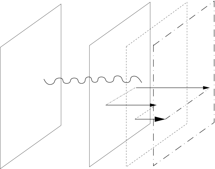
Figure 6: One brane is gravitationally interacting with 3 parallel branes which interact among themselves with 3 open strings.

Figure 7: The previous figure interpreted in the open channel.

$${\cal A}_{N~{}tach,1~{}loop} = \langle Dp|\Delta_{c}|Dp,\{N\}\rangle\prod_{1\leq i\leq N}|k_{i}\rangle$$ (4.73)

$$= \langle Dp|\Delta_{c}|Dp,\{k_{i}\}_{\{1\leq i\leq N\}}\rangle$$

$$= {\cal N}^{N}_{o(p)}\left(\frac{T_{p}}{2}\right)^{2}~{}\langle Dp|~{}e^{-i\alpha(p)}~{}\frac{\alpha^{\prime}\pi}{2}\int_{0}^{\infty}d\tau e^{-\pi\tau(L_{0}+\tilde{L}_{0}-2)}\delta_{L_{0},\tilde{L}_{0}}$$

$$e^{i\alpha(p)}~{}2\pi i\int_{0}^{2\pi}\prod_{i=1}^{N-1}\theta(\phi_{i}-\phi_{i+1})de^{i\phi_{i}}\prod_{i<j}(e^{i\phi_{i}}-e^{i\phi_{j}})^{2\alpha^{\prime}k_{i}\cdot k_{j}}$$

$$e^{i\sum_{i}k_{i}\cdot X^{(c)(-)}_{L}(e^{i\phi_{i}})}e^{i\sum_{j}k_{j}\cdot X^{(c)(+)}_{L}(e^{i\phi_{j}})}e^{-i\sum_{i}k_{i}\cdot\left(\frac{x_{L}-Sx_{R}}{2}{}\right)}|Dp\rangle$$

where $\phi_{N}=0$ and $|Dp\rangle$ is the plain boundary state associated with a $Dp$ brane with boundary conditions dictated by the reflection matrix $S$. A straightforward computation gives

$${\cal A}_{N~{}tach,1~{}loop}=$$

$$= (2\pi)^{2}i\frac{\alpha^{\prime}}{4}{\cal N}^{N}_{o(p)}\left(\frac{T_{p}}{2}\right)^{2}\int_{0}^{\infty}d\tau\int_{0}^{2\pi}\prod_{i=1}^{N-1}de^{i\phi_{i}}~{}\theta(\phi_{i}-\phi_{i+1})$$

$$\left[2\pi\delta(\sum_{i}k_{i}^{\nu})\right]^{D_{NN,nc}}\times\delta_{\sum_{i}k_{i}^{\delta}}^{D_{DD,nc}}\left(\frac{2}{\alpha^{\prime}\tau}\right)^{D_{DD,nc}/2}e^{-\frac{2}{\alpha^{\prime}\tau}\left(y_{\pi}^{\delta}-y_{0}^{\delta}+\alpha^{\prime}\sum_{i}k_{i}^{\delta}\phi_{i}\right)^{2}}$$

$$\delta_{\sum_{i}k_{i}^{n}}^{D_{NN,c}}\sum_{w}e^{-\frac{1}{2}\pi\alpha^{\prime}\tau\left(\frac{w^{n}R}{\alpha^{\prime}}\right)^{2}}e^{i\frac{wR}{\alpha^{\prime}}\left(y_{\pi}^{n}-y_{0}^{n}+\alpha^{\prime}\sum_{i}k_{i}^{n}\phi_{i}\right)}\times\delta_{\sum_{i}k_{i}^{d}}^{D_{DD,c}}\sum_{n}e^{-\frac{1}{2}\pi\alpha^{\prime}\tau\left(\frac{n}{R}\right)^{2}}e^{i\frac{n}{R}\left(y_{\pi}^{d}-y_{0}^{d}+\alpha^{\prime}\sum_{i}k_{i}^{d}\phi_{i}\right)}$$

$$\left(\prod_{n=1}^{\infty}\frac{1}{1-e^{-2\pi\tau n}}\right)^{D-2}\times\prod_{i<j}\left(\prod_{m=1}^{\infty}\frac{1-2\cos\phi_{ij}~{}e^{-2\pi\tau m}+e^{-4\pi\tau m}}{(1-e^{-2\pi\tau m})^{2}}\right)^{2\alpha^{\prime}k_{i}\cdot k_{j}}(e^{i\phi_{i}}-e^{i\phi_{j}})^{2\alpha^{\prime}k_{i}\cdot k_{j}}$$

(4.74)

where the first two terms in the last line are due to non zero modes (the ghosts account for the $-2$ in the exponent $D-2$) with $\phi_{ij}=\phi_{i}-\phi_{j}$, in last but one line we have the compact zero modes contributions and in the third line there are the contributions from non compact zero modes: the non compact contribution from DD directions must again be understood as the decompactification limit since we otherwise would miss the conservation of distances which is a Kronecker delta and not a Dirac delta. As before we have used the index $n$ ($\nu$) for (non) compact NN directions and $d$ ($\delta$) for (non) compact DD ones.

In eq. (4.74) the contribution from non zero modes was easily computed using

$$\langle 0,\tilde{0}|e^{-s_{0}a\tilde{a}}e^{a^{\dagger}A}e^{aB}e^{-s_{\pi}a^{\dagger}\tilde{a}^{\dagger}}|0,\tilde{0}\rangle=\frac{1}{1-s_{0}s_{\pi}}e^{\frac{ABs_{0}s_{\pi}}{1-s_{0}s_{\pi}}}$$ (4.75)

The string amplitude (4.74) for the special case of $D25$ ($S={\hbox{1\kern-3.00003pt1}}$) with all non compact directions reduces to the well know 1 loop $N$ tachyons open string amplitude:

$${\cal A}_{N~{}tach,1~{}loop}=$$

$$= {\cal C}_{1(25)}{\cal N}^{N}_{o(25)}(2\pi)^{26}\delta^{26}(\sum_{i}k_{i}^{\nu})~{}\int_{0}^{\infty}d\tau\frac{2\pi}{2}\int_{0}^{2\pi}\prod_{i=1}^{N-1}\frac{d\phi_{i}}{2}~{}\theta(\phi_{i}-\phi_{i+1})$$

$$\left(\prod_{n=1}^{\infty}\frac{1}{1-e^{-2\pi\tau n}}\right)^{D-2}\times\prod_{i<j}\left(\sin\frac{\phi_{ij}}{2}\prod_{m=1}^{\infty}\frac{1-2\cos\phi_{ij}~{}e^{-2\pi\tau m}+e^{-4\pi\tau m}}{(1-e^{-2\pi\tau m})^{2}}\right)^{2\alpha^{\prime}k_{i}\cdot k_{j}}$$

(4.76)

upon the use of momentum conservation, mass shell condition $\alpha^{\prime}k_{i}^{2}=1$, $2\alpha^{\prime}\sum_{i<j}k_{i}\cdot k_{j}=-N$ and $\phi_{N}=0$ to write

$$\prod_{k=1}^{N-1}d{e^{i\phi_{k}}}\prod_{1\leq i<j\leq N}(e^{i\phi_{i}}-e^{i\phi_{j}})^{2\alpha^{\prime}k_{i}\cdot k_{j}}$$ (4.77)

$$= \prod_{k=1}^{N-1}d{e^{i\phi_{k}}}\prod_{i<j}\left[e^{i\frac{\phi_{i}+\phi_{j}}{2}2\alpha^{\prime}k_{i}\cdot k_{j}}(2i~{}\sin\frac{\phi_{ij}}{2})^{2\alpha^{\prime}k_{i}\cdot k_{j}}\right]$$

$$= \prod_{k=1}^{N-1}~{}d{\phi_{k}}\prod_{i<j}(2i~{}\sin\frac{\phi_{ij}}{2})^{2\alpha^{\prime}k_{i}\cdot k_{j}}=\frac{1}{2i}\prod_{k=1}^{M-1}\frac{d{\phi_{k}}}{2}\prod_{i<j}(\sin\frac{\phi_{ij}}{2})^{2\alpha^{\prime}k_{i}\cdot k_{j}}$$

5 Conclusions.

In this article we have shown how to compute boundary states which describe $N$ parallel branes in generic position, i.e. not superimposed, interacting through $N$ open string states in eq. (4.54). We have also computed the corresponding boundary states when the branes are superimposed as in eq.(4.62).

The result is not completely unexpected but there are some points which are not trivial:

• when acting on the trivial boundary state with open string vertex operators we have to substitute $X_{open}$ with the left moving part of the closed string $X_{L}$ in order to obtain a T-duality invariant formulation;

• the non compact Dirichlet directions must be treated as a decompactification limit;

• in compact directions we have to equally divide the momenta coming from open string vertices between left and right closed string momenta, as it is explicit in eq. (4.54).

Another point which is worth noticing is that this derivation is valid for the bosonic free string but this could be in principle extended to other CFTs since the fundamental starting point is the possibility of writing the closed string vertices as a product of two open string ones. This possibility is quite natural when one starts from the open string $\sigma$ model as discussed around eq. (2.7): in particular this is clear for the bosonic/ NS-NS gravitational sector which couples universally in both bosonic and fermionic strings but it is also true for the fermionic and RR sectors where branes couple only to a subsector of all the possible closed string states.

Acknowledgments

The author thanks M. Billó and A. Lerda for discussions and the Niels Bohr Institute for the hospitality during the completion of this paper. This work supported in part by the European Community’s Human Potential Program under contract HPRN-CT-2000-00131 Quantum Spacetime. It is also partially supported by the Italian MIUR under the program “Teoria dei Campi, Superstringhe e Gravitá”.

Appendix A Conventions.

• Indices:
  $\alpha=0\dots{\hat{d}}-1$ for non compact directions and $a={\hat{d}}\dots D-1$ for compact ones; $n$ ($\nu$) for (non) compact NN directions and $d$ ($\delta$) for (non) compact DD ones.

• Amplitudes normalizations.
  If the $d$ dimensional YM action is given by $S_{YM}=\int d^{d}x~{}tr(F_{\mu\nu}F^{\mu\nu})$ with $F_{\mu\nu}=\partial_{\mu}A_{\nu}-\partial_{\nu}A_{\mu}-ig_{d}[A_{\mu},A_{\nu}]$, $A_{\mu}=A_{\mu}^{a}\lambda^{a}$ and $tr(\lambda^{a}\lambda^{b})=\frac{1}{2}\delta^{ab}$, $tr(\lambda^{a}[\lambda^{b},\lambda^{c}])=\frac{i}{2}f^{abc}$, it is possible to derive from direct comparison with field theory as in ref. [11]

  $${\cal N}_{o(d-1)}=g_{d}\sqrt{2\alpha^{\prime}}\,\,,\,\,{\cal C}_{0(d-1)}=\frac{1}{(g_{d}\alpha^{\prime})^{2}}\,\,,\,\,\frac{{\cal C}_{h+1(d-1)}}{{\cal C}_{h(d-1)}}=\frac{(g_{d}\alpha^{\prime})^{2}}{(2\pi)^{d}(2\alpha^{\prime})^{d/2}}$$

  and from unitarity

  $${\cal C}_{0(d-1)}{\cal N}_{o(d-1)}^{2}\alpha^{\prime}=2$$

  when using $\Delta_{o}=\int_{0}^{1}dx~{}x^{L_{0}-2}$ ($L_{0}=\alpha^{\prime}p^{2}+\sum_{1}^{\infty}na^{\dagger}_{n}\cdot a_{n}$). In a similar way it follows from closed string unitarity

  $${\cal\widehat{C}}_{0}{\cal\widehat{N}}_{c}^{2}\alpha^{\prime}=4\pi$$

  when using as closed string propagator $\Delta_{c}=\frac{\alpha^{\prime}}{4\pi}\int_{|z|<1}\frac{d^{2}z}{|z|^{2}}z^{L_{0}-1}{\bar{z}}^{\tilde{L}_{0}-1}$ ($L_{0}=\alpha^{\prime}p_{L}^{2}+\sum_{1}^{\infty}na^{\dagger}_{n}\cdot a_{n}$, $\tilde{L}_{0}=\alpha^{\prime}p_{R}^{2}+\sum_{1}^{\infty}n\tilde{a}^{\dagger}_{n}\cdot\tilde{a}_{n}$, ).

  The vertex normalization factors ${\cal N}_{o(d-1)}$, ${\cal N}_{c}$ and ${\cal\widehat{N}}_{c}$ are common to all the states but depend on the number of compact and non compact directions.

• Vacua normalizations in non compact directions.
  For each non compact direction of open string with NN b.c. or of closed string: $\langle k|k^{\prime}\rangle=2\pi\delta(k-k^{\prime})$ with $\langle k|=|k\rangle^{\dagger}$, $|x=0\rangle\equiv\delta(x)|p=0\rangle$,

  For each non compact direction with DD b.c. since only $|0\rangle$ has finite energy: $\langle 0|0\rangle=1$ but the spectral decomposition of the unity is ${\hbox{1\kern-3.00003pt1}}=\lim_{R\rightarrow\infty}\sum_{w}|w\rangle\langle w|$; For each compact direction $\langle n|m\rangle=\delta_{n,m}$.

• $z\in{\hbox{l\kern-5.406ptC}}\Leftrightarrow-\pi<arg(z)\leq\pi$, $z\in{\hbox{l\kern-5.406ptH}}^{+}\Leftrightarrow 0\leq arg(z)\leq\pi$

• Open string modes expansions:

  $$X(z,\bar{z})=\frac{1}{2}\left(X_{L}(z)+X_{R}(\bar{z})\right)$$

  $$X^{\mu}_{L/R}(z)=q^{\mu}\pm y^{\mu}_{0}-{\rm i}\,\sqrt{2\alpha^{\prime}}\,a_{0}^{\mu}{}\ln z+{\rm i}\,\sqrt{2\alpha^{\prime}}\,\sum_{n\not=0}{sgn(n)\over{\sqrt{|n|}}}a_{n}^{\mu}z^{-n}$$

  where $z=e^{\tau_{E}+i\sigma}\in{\hbox{l\kern-5.406ptH}}^{+}$ ($\tau_{E}$ is the Wick rotated time) and the logarithm entering the string expansion is defined to have a cut at $arg(z)=-\pi$, i.e. $-\pi<arg(z)\leq+\pi$ moreover $log(\bar{z})\equiv\overline{log(z)}$ and $a^{\mu}_{0}=\sqrt{2\alpha^{\prime}}p^{\mu}$ in the NN case.

  The commutation relations are ( $a_{-n}=a_{n}^{\dagger}$)

  $$[q^{\mu},p^{\nu}]=i\eta^{\mu\nu}~{}~{}~{}~{}[a_{m}^{\mu},a^{\dagger\nu}_{n}]=\delta_{m,n}\eta^{\mu\nu}~{}~{}m,n>0$$

  The spectrum of the momentum operator is

  $$k=\left\{\begin{array}[]{ll}k^{\alpha}&\textrm{non compact NN bc}\\ \frac{n^{n}+\theta_{0}^{n}-\theta_{\pi}^{n}}{R}&\textrm{compact NN bc}\\ \frac{y_{\pi}^{\delta}-y_{0}^{\delta}}{2\pi\alpha^{\prime}}&\textrm{non compact DD bc}\\ \frac{w^{d}~{}R}{\alpha^{\prime}}+\frac{y_{\pi}^{d}-y_{0}^{d}}{2\pi\alpha^{\prime}}&\textrm{compact DD bc}\end{array}\right.$$

  where $y_{0}$ ($y_{\pi}$) is the position of the brane at $\sigma=0$ ($\sigma=\pi$) and $2\pi\theta_{0}^{n}$ ($2\pi\theta_{\pi}^{n}$) is the Wilson line on the brane at $\sigma=0$ ($\sigma=\pi$).

• The closed string modes expansion is given in analogous manner by

  $$X(z,\bar{z})=\frac{1}{2}\left(X^{(c)}_{L}(z)+{\tilde{X}^{(c)}_{R}}(\bar{z})\right)$$

  where now $z=e^{2\tau_{E}+2i\sigma}\in{\hbox{l\kern-5.406ptC}}$, $X^{(c)}_{L}$ has the same expansion as for the open string but with $y_{0}=0$ and ${\tilde{X}}_{R}^{(c)}$ expands as $X_{L}^{(c)}$ but with tilded operators, the commutation relations read

  $$[q_{L}^{\mu},p_{L}^{\nu}]=[q_{R}^{\mu},p_{R}^{\nu}]=i\eta^{\mu\nu}~{}~{}~{}~{}[a_{Lm}^{\mu},a^{\dagger\nu}_{Ln}]=[\tilde{a}_{Rm}^{\mu},\tilde{a}^{\dagger\nu}_{Rn}]=\delta_{m,n}\eta^{\mu\nu}~{}~{}m,n>0$$

  In the non compact case we identify $x_{L}=x_{R}=x$ and $p_{L}=p_{R}=\frac{p}{2}$ where $p$ has continuum spectrum while in compact directions $p_{L}$ ($p_{R}$) has discrete spectrum given by $k_{L}=\frac{1}{2}\left(\frac{n}{R}+\frac{wR}{\alpha^{\prime}}\right)$ ($k_{R}=\frac{1}{2}\left(\frac{n}{R}-\frac{wR}{\alpha^{\prime}}\right)$).

Appendix B Phases and Analytic continuations.

We start writing the three Reggeon Sciuto-Della Selva-Saito vertex ([16]) for a single coordinate

$$S(z)=:\exp\left(-\frac{1}{2\alpha^{\prime}}\oint_{u=0,|u|<|z|}\frac{du}{2\pi i}X_{aux}(u+z)\partial_{u}X(u)\right):$$ (B.78)

where the normal ordering is taken with respect to both the auxiliary $X_{aux}$ and the usual $X(u)\equiv X_{L}(u)$. Performing the integral over $u$ the previous equation becomes ($\sqrt{0}\equiv 1$)

$$S(z)=:\exp\left(\frac{i}{\sqrt{2\alpha^{\prime}}}\sum_{n=0}^{\infty}\frac{\sqrt{n}\,a_{n}}{n!}\partial^{n}X_{aux}(z)\right):$$ (B.79)

This vertex can be thought of as a generating functional of all vertices :

$$\langle 0_{a},x=0|\,S(z)\,|\alpha,k\rangle=V_{\alpha}^{(aux)}(z;k)$$ (B.80)

We use this formalism in order to exam in general the phases occurring when performing the analytic continuation of the product of two such vertices. We first compute the product of two SDS vertices

$$S(z)\,S(w)\,\, = \,:S(z)\,S(w)\,$$

$$e^{-\frac{1}{2\alpha^{\prime}}\oint_{u=0}\frac{du}{2\pi i}\oint_{v=0,|v-u|<|z-w|}\frac{dv}{2\pi i}\log\left(z-w+u-v\right)\partial X_{(1)}(u)\partial X_{(2)}(v)}:$$

$$= \,:S(z)\,S(w)\,e^{\log(z-w)\,2\alpha^{\prime}\,p^{(1)}p^{(2)}}...:\,\,\,\,|z|>|w|$$

in this expression the $log$ has to be interpreted as a shorthand version of

$$\log\left(z-w+u-v\right)\equiv\log(z)-\sum_{n=1}^{\infty}\frac{1}{n}\left(\frac{w}{z}\right)^{n}-\sum_{n=1}^{\infty}\frac{1}{n}\left(\frac{v-u}{z-w}\right)^{n}$$

and we have made use of the well known expression

$$X(z)X(w)=:X(z)X(w):-2\alpha^{\prime}\,\log(z-w)\,\,\,\,|z|>|w|$$ (B.82)

Then we compare this equation (B) with the analogous product $S(w)\,S(z)$ for $|z|<|w|$ and we use

$$\left[\log(z-w)\right]_{an.~{}cont.}=\log(w-z)+i\pi~{}sign(arg(z)-arg(w))~{}~{}~{}~{}-\pi<arg(z),arg(w)<\pi$$ (B.83)

we get the desired phase

$$\left[S(z)\,S(w)\right]_{an.cont}=S(w)\,S(z)e^{+i\pi\,sgn(arg(z)-arg(w))\,2\alpha^{\prime}\,p_{0(1)}p_{0(2)}}$$ (B.84)

with $-\pi<arg(z),arg(w)\leq+\pi$. In the generic case the phase of the previous equation becomes

$$\pi\,sgn(arg(z)-arg(w))\Rightarrow 2\pi(n_{z}-n_{w})+\pi\,sgn([\phi_{z}]-[\phi_{w}])$$ (B.85)

where we have defined $arg(z)=[\phi_{z}]+2\pi n_{z}$ with $-\pi<[\phi_{z}]\leq\pi$ and $n_{z}\in{\mathchoice{\hbox{Z\kern-4.2679ptZ}}{\hbox{Z\kern-4.2679ptZ}}{\hbox{{Z\kern-3.41432ptZ}}}{\hbox{{Z\kern-3.41432ptZ}}}}$.

Appendix C Details on the cocycles computations.

C.1 Closed string case.

In this section we give the details on the derivation of the closed string cocycles. In section (3.1) we introduced the phase $e^{i\Phi_{(c)}(k_{1},k_{2})}$ as the phase which arises when computing the normal ordering of the product of two closed string vertices $\cal W$, explicitly

$${\cal W}^{(c)}_{\beta_{L},\beta_{R}}(z,\bar{z};k_{1}){\cal W}^{(c)}_{\alpha_{L},\alpha_{R}}(w,\bar{w};k_{2}) = e^{i\Phi_{(c)}(k_{1},k_{2})}c(k_{L1}+k_{L2},k_{R1}+k_{R2};p_{L},p_{R})*$$

$$V_{\beta_{L}}(z;k_{L1})V_{\alpha_{L}}(w;k_{L2})\,\,\,\,{\tilde{V}}_{\beta_{R}}({\bar{z}};k_{R1}){\tilde{V}}_{\alpha_{R}}({\bar{w}};k_{R2})$$

with

$$\Phi_{(c)}(k_{1},k_{2}) = -\pi\,\alpha^{\prime}\left[\left({\cal B}\,k_{L2}+{\cal C}\,k_{R2}\right)\cdot k_{L1}+\left({\cal D}\,k_{L2}+{\cal E}\,k_{R2}\right)\cdot k_{R1}\right]$$ (C.87)

where the matrices ${\cal B},{\cal C},{\cal D}$ and ${\cal E}$ may only have non vanishing entries in compact directions, i.e. for example ${\cal B}^{a}_{b}$.

With the help of the well known formula ($-\pi\leq arg(z),arg(w)\leq+\pi$, $|z|<|w|$) (see also app. B)

$$\left[V(z;k_{1})\,V(w;k_{2})\right]_{\mbox{an.con.}}=V(w;k_{2})\,V(z;k_{1})e^{+i\pi\,sgn(arg(z)-arg(w))\,2\alpha^{\prime}\,k_{1}\cdot k_{2}}$$

and by comparing with the analogous product of the vertices in the opposite order

$${\cal W}^{(c)}_{\alpha_{L},\alpha_{R}}(w,\bar{w};k_{2}){\cal W}^{(c)}_{\beta_{L},\beta_{R}}(z,\bar{z};k_{1})$$

it is not difficult to see that the constraint we want to impose on the cocycles coefficients in order to implement the commutativity is

$$e^{i\Phi_{(c)}(k_{1},k_{2})-i\Phi_{(c)}(k_{2},k_{1})+i\pi sgn(arg(z)-arg(w))2\alpha^{\prime}(k_{L1}\cdot k_{L2}-k_{R1}\cdot k_{R2})}=$$

$$e^{-i\pi\,\alpha^{\prime}\left[({\cal B}-{\cal B}^{T})k_{L2}\cdot k_{L1}+({\cal E}-{\cal E}^{T})k_{R2}\cdot k_{R1}\right]}\times$$

$$e^{-i\pi\,\alpha^{\prime}\left[({\cal C}-{\cal D}^{T})k_{R2}\cdot k_{L1}-({\cal C}-{\cal D}^{T})^{T}k_{L2}\cdot k_{R1}-2sgn(arg(z)-arg(w))(k_{L1}\cdot k_{L2}-k_{R1}\cdot k_{R2})\right]}=1$$

The quantities entering the previous equation can be trivially evaluated, in particular for any compact direction we have

$$2\alpha^{\prime}\,(k_{L1}^{a}k_{R2}^{b}-k_{R1}^{a}k_{L2}^{b})=w_{1}^{a}n_{2}^{b}\frac{R^{a}}{R^{b}}-w_{2}^{b}n_{1}^{a}\frac{R^{b}}{R^{a}}\,\,,\,\,2\alpha^{\prime}\,(k_{L1}^{a}k_{L2}^{b}-k_{R1}^{a}k_{R2}^{b})=w_{1}^{a}n_{2}^{b}\frac{R^{a}}{R^{b}}+w_{2}^{b}n_{1}^{a}\frac{R^{b}}{R^{a}}$$ (C.89)

Considering the cases where the momentum and winding are different from zero only in a given compact direction $a$ we deduce immediately that we have to impose the following restriction on the coefficients entering the cocycles definition (3.15)

$$({\cal C}-{\cal D}^{T})_{aa}=4{N_{a}}+2\,\,\,\,{N_{a}}\in{\mathchoice{\hbox{Z\kern-4.2679ptZ}}{\hbox{Z\kern-4.2679ptZ}}{\hbox{{Z\kern-3.41432ptZ}}}{\hbox{{Z\kern-3.41432ptZ}}}},$$ (C.90)

and

$${\cal B}_{aa},{\cal E}_{aa}\in R~{}.$$ (C.91)

If we consider the cases where only two compact directions have $k_{L/R}\neq 0$ and we choose their radii not to be equal we deduce that the off-diagonal elements must be identically zero:

$$({\cal C}-{\cal D}^{T})_{ab} = 0~{}~{}~{}~{}(a\neq b)$$

$${\cal B}_{ab} = {\cal E}_{ab}=0~{}.$$ (C.92)

A further constraint comes from hermitian property of the vertex: the hermitian of a vertex is given by the following expression

$$\left[{\cal W}^{(c)}_{\beta_{L},\beta_{R}}(z,\bar{z};k)\right]^{\dagger}=e^{i\Phi_{(c)}(k,k)}\frac{1}{|z|^{2}}{\cal W}^{(c)}_{\beta_{L},\beta_{R}}(\frac{1}{\bar{z}},\frac{1}{z};-k)$$ (C.93)

from which we find

$$e^{i\Phi_{(c)}(k,k)} = e^{-i\pi\,\alpha^{\prime}\left[{\cal B}\,k_{L}\cdot k_{L}+({\cal C}+{\cal D}^{T})\,k_{R}\cdot k_{L}+{\cal E}\,k_{R}\cdot k_{R}\right]}$$ (C.94)

$$= e^{-i\pi\,\alpha^{\prime}\left[{\cal B}_{aa}\,k_{La}^{2}+({\cal C}+{\cal D}^{T})\,k_{Ra}k_{La}+{\cal E}_{aa}\,k_{Ra}^{2}\right]}$$

$$= e^{-i\pi\,\alpha^{\prime}[{\cal B}+{\cal E}+({\cal C}+{\cal D})]_{aa}\left(\frac{n_{a}}{R}\right)^{2}}~{}e^{-i\pi\,\alpha^{\prime}[{\cal B}+{\cal E}-({\cal C}+{\cal D})]_{aa}\left(\frac{w_{a}R}{\alpha^{\prime}}\right)^{2}}~{}e^{-i\pi\,[{\cal B}-{\cal E}]_{aa}n_{a}w_{a}}$$

$$= 1$$

and finally

$${\cal C}_{aa}=-{\cal D}_{aa}=1+2N_{a}~{}~{}~{}~{}~{}{\cal B}_{aa}=-{\cal E}_{aa}=2M_{a}$$ (C.95)

where $M_{a}$ are arbitrary integers. In the text we will use

$$N_{a}=0~{}~{}~{}~{}M_{a}=0$$ (C.96)

Further constraints come from unitarity which requires that any three points amplitude ${\cal A}(1,2,3)$ be connected with the amplitude ${\cal A}(-1,-2,-3)$ for the CPT conjugate particles ($(-1)$ means the CPT conjugate state of $1$) by

$${\cal A}(1,2,3)=\left({\cal A}(-1,-2,-3)\right)^{*}$$ (C.97)

This equation can be specialized to the case of three tachyons with momenta $k_{i}=(k^{\alpha}_{i},(k^{a}_{Li},k^{a}_{Ri}))$ ($i=1,2,3$) and results in

$${\cal A}(T_{1},T_{2},T_{3})\propto e^{i\sum_{1\leq i\leq j\leq 3}\Phi_{(c)}(k_{i},k_{j})}\delta^{d}(\sum k^{\alpha}_{i})\delta_{\sum k_{Li}}\delta_{\sum k_{Ri}}$$ (C.98)

If we consider sequentially configurations with only one winding, two windings different from zero, analogously for momenta and finally configurations with mixed momenta and windings and we require a smooth behavior of the cocycles in the large and small $R_{a}$ limits we get the results given in the main text.

C.2 Open string computation.

In this appendix we give the details on how to obtain eq.s (LABEL:VV-0,3.23) and eq. (3.24). To this purpose we write the generic closed string emission vertex in open string formalism with the cocycles as

$${\cal W}_{\beta_{L},\beta_{R}}(z,\bar{z};k) = c(k_{L},k_{R},p){V}_{\beta_{L}}(X_{L}(z);k_{L}){}~{}{V}_{\beta_{R}}(X_{R}(\bar{z});k_{R})$$ (C.99)

with

$$c(k_{L},k_{R},p) = c_{nop}(k_{L},k_{R})c_{op}(k_{L},k_{R};p)$$

$$c_{op}(k_{L},k_{R};p) = e^{i\pi\,\alpha^{\prime}(uk_{L}+vk_{R})\cdot p}$$ (C.100)

$$c_{nop}(k_{L},k_{R}) = e^{i\pi\alpha^{\prime}\,(\eta k_{L}\cdot k_{L}+\gamma k_{L}\cdot k_{R}+\epsilon k_{R}\cdot k_{R})},~{}~{}~{}~{}\eta^{T}=\eta,~{}\gamma^{T}=\gamma$$ (C.101)

where $c_{op}$ ($c_{nop}$) is the (non) operatorial part of the cocycle and $k_{L}=k_{R}=\frac{k}{2}$ in non compact direction. Our aim is now to determine the (matrix) coefficients $u,v,\eta,\gamma,\epsilon$ in order to reproduce the commutativity, the “OPE” coefficients in eq. (3.1) or eq. (LABEL:OPE_phase_closed_app0) and the behavior of closed string vertices under hermitian conjugation (C.93). It is worth stressing that the previous expression for the cocycles (C.101) contains a contribution from all directions, even the directions with $DD$ boundary condition since the $\sigma$ coefficient in the string modes expansion is an operator and hence commuting the cocycles with $X_{L/R}$ yields a non trivial phase. If compute the phase which we obtain normal ordering the product of two vertices as done in (3.1) and we remember that $X_{R}=SX_{R}^{NN}$ (where $X_{R}^{NN}$ is the right moving part with NN boundary conditions) we get

$$e^{i\Phi_{(o)}(k_{1},k_{2})}=\frac{c_{nop}(k_{1})c_{nop}(k_{2})}{c_{nop}(k_{1}+k_{2})}e^{-i\pi\alpha^{\prime}(uk_{L2}+vk_{R2})\cdot(k_{L1}+Sk_{R1})}e^{-i2\pi\alpha^{\prime}Sk_{R1}\cdot k_{L2}}$$ (C.102)

In this expression the first factor of rhs is due to non operatorial cocycles, the second to the reordering of the operatorial ones and the last to the reordering of $V_{R}(k_{R1})V_{L}(k_{L2})$. We require then that the closed string phase (C.87) in closed string formalism and the corresponding phase (C.102) in open string formalism be equal, i.e.

$$e^{i\Phi_{(o)}(k_{1},k_{2})}=e^{i\Phi_{(c)}(k_{1},k_{2})}$$ (C.103)

which is the necessary condition for the correct factorization of mixed open/closed string amplitudes in the closed channel. Given this basic constraint (C.103) we can check that the further constraints which arise from requiring the commutativity of two closed string vertices and the proper behavior under hermitian conjugation are identically satisfied. In particular the phase which arises when computing the hermitian of a vertex is $\Phi_{(o)}(k,k)$ analogously to what we have found with the closed string formalism (C.93).

The constraint (C.103) can be explicitly rewritten as

$$e^{-i\pi\,\alpha^{\prime}\left[\left({\cal B}\,k_{L2}+{\cal C}\,k_{R2}\right)\cdot k_{L1}+\left({\cal D}\,k_{L2}+{\cal E}\,k_{R2}\right)\cdot k_{R1}\right]}=$$

$$e^{-i\pi\,\alpha^{\prime}\left[2\eta k_{L1}\cdot k_{L2}+2\epsilon k_{R1}\cdot k_{R2}+\gamma k_{L1}\cdot k_{R2}+\gamma k_{L2}\cdot k_{R1}+(uk_{L2}+vk_{R2})\cdot(k_{L1}+Sk_{R1})+2Sk_{R1}\cdot k_{L2}\right]}$$

By considering different combinations of windings and momenta as done for the closed string cocycles after eq. (C.1) and using eq.s (C.89) we derive the following constraints:

$$\left(2\eta+(1+S)u+2S\right)_{\alpha\beta}=0,\,\,\,\,\gamma_{\alpha\beta}=\epsilon_{\alpha\beta}=v_{\alpha\beta}=0$$ (C.104)

(up to a “gauge” choice which allows to set $\gamma=\epsilon=v=0$) for matrix indexes in the non compact directions and

$$||\left(2\eta+u-{\cal B}\right)_{ab}||=||\left({\cal E}-2\epsilon-Sv\right)_{ab}||=2\,diag(\widehat{M}_{a}+2\widehat{D}_{a})$$ (C.105)

for $k_{L1a}k_{L2b}$ and $-k_{R1a}k_{R2b}$ coefficients in compact directions and

$$||\left(\gamma^{T}+v-{\cal C}\right)_{ab}||=||-\left(-{\cal D}+\gamma+Su+2S\right)_{ab}||=2\,diag(\widehat{M}_{a})$$

(C.106)

for $k_{L1a}k_{R2b}$ and $-k_{R1a}k_{L2b}$ coefficients. The $\widehat{M}_{a}$ are arbitrary integers because of eq.s (C.89). Consistency of the two last equations (C.106) for $\gamma$ implies that

$$v-(Su)^{T} = 2+2S+4\hat{M}+4N$$ (C.107)

Next we want to exam the open string/closed string vertices commutativity. To this purpose we write the open string emission vertex from the $\sigma=0$ boundary as

$${\cal V}_{\alpha}(x;k)=e^{i\pi\alpha^{\prime}\,\tilde{u}k\cdot p}{V}_{\alpha}(X_{L}(x){-y_{0}};k)\,~{}~{}~{}~{}x>0$$ (C.108)

where $\tilde{u}$ is an unknown matrix. The naive way of writing this commutativity condition (which is wrong!)

$$\left[{\cal W}_{\beta_{L},\beta_{R}}(X_{L}(z),X_{R}(\bar{z}))\,{\cal V}_{\alpha}(x;k)\right]_{an.con.} = {\cal V}_{\alpha}(x;k)\,{\cal W}_{\beta_{L},\beta_{R}}(X_{L}(z),X_{R}(\bar{z}))$$

implies that

$$e^{i\pi\alpha^{\prime}\left[(uk_{L}+vk_{R})\cdot k+2k\cdot(k_{L}-Sk_{R})-\tilde{u}k\cdot(k_{L}+Sk_{R})\right]}=1$$ (C.109)

which can be satisfied when

$$\left(-u+\tilde{u}^{T}(1+S)-2(1-S)\right)_{\alpha\beta} = 0$$ (C.110)

$$\left(u-\tilde{u}^{T}+2\right)_{ab}=\left(v-(\tilde{u}^{T}+2)S\right)_{ab} = 0$$ (C.111)

respectively for matrix indices in non compact and compact directions. In particular the equations in the last line arise since eq. (C.109) must be valid also when Wilson lines are turned on, i.e. when $k=\frac{n+\theta}{R}$.

In a similar way we get further constraints requiring that the generic vertex for the open string emission from the $\sigma=\pi$ border

$${\cal V}_{\alpha}(-x;k)=e^{i\pi\alpha^{\prime}\,\tilde{u}_{\pi}k\cdot p}{V}_{\alpha}(X_{L}(-x){-y_{0}};k)$$ (C.112)

commute with both closed string and $\sigma=0$ open string vertices.

The coefficient $\tilde{u}_{\pi}$ can be fixed by requiring the commutativity of $\sigma=\pi$ open string vertices the with $\sigma=0$ open string vertices; it turns easily out that

$$\tilde{u}_{\pi}=\tilde{u}-2$$ (C.113)

This in turn implies that the commutativity of an open string emission vertex from $\sigma=\pi$ with a closed string vertex does not really yield new constraints but some consistency conditions which read

$$\left(-u+\tilde{u}^{T}(1+S))\right)_{\alpha\beta} = 0$$ (C.114)

$$\left(u-\tilde{u}^{T}\right)_{ab}=\left(v-\tilde{u}^{T}S\right)_{ab} = 0$$ (C.115)

Unfortunately or better correctly the sets of constraints (C.110-C.111) and (C.114-C.115) are inconsistent. This would seem to be a disaster but luckily it is not so since the proper way of formulation open/closed string commutativity reads, as explained in the main text, is to take into account the $y_{0}$ shift so that

$$\left[{\cal W}_{\beta_{L},\beta_{R}}(X_{L}^{out}(z),X_{R}^{out}(\bar{z}))\,{\cal V}_{\alpha}(x;k)\right]_{an.con.} = {\cal V}_{\alpha}(x;k)\,{\cal W}_{\beta_{L},\beta_{R}}(X_{L}^{in}(z),X_{R}^{in}(\bar{z}))$$

$$= {\cal V}_{\alpha}(x;k)\,{\cal W}_{\beta_{L},\beta_{R}}(X_{L}^{out}(z),X_{R}^{out}(\bar{z}))e^{2\pi\alpha^{\prime}i\,k\cdot(k_{L}-Sk_{R})}$$

As a consequence of this proper commutativity condition all the constraints from open/closed string vertices commutativity are now consistent and turn out to be eq.s (C.115) because of the extra phase contribution from the proper commutativity condition.

From hermiticity conjugation of ${\cal V}_{\alpha}$ vertices we get

$$\tilde{u}+\tilde{u}^{T}=0$$ (C.116)

which gives using eq.s (C.114), (C.115) and the consistency condition (C.107)

$$\tilde{u}=u=v=0~{}~{}~{}~{}~{}~{}2\widehat{M}+2N+{1+S}=0$$ (C.117)

Finally using eq.s (C.95) we get

$$\gamma = ({\cal C}+2\widehat{M})^{T}=(1+2N+2\widehat{M})^{T}=-S$$

$$\eta = -\epsilon=\frac{1}{2}{\cal B}+\widehat{M}+2\widehat{D}=-\frac{1}{2}{\cal E}+\widehat{M}+2\widehat{D}=M+\widehat{M}+2\widehat{D}$$ (C.118)

With our choice (C.96) and choosing $\widehat{M}=\widehat{D}=0$ we finally find

$$\gamma=-S,~{}~{}~{}~{}\eta=-\epsilon=0$$ (C.119)

It is interesting to notice that the hermiticity of the open string vertices ${\cal V}_{\alpha}(-x)$ does not yield any further constraint since the phase $e^{i2\pi\alpha^{\prime}k^{2}}$ which is obtained reordering the cocycle $e^{i\pi\alpha^{\prime}\,\tilde{u}_{\pi}k\cdot p}$ after taking the hermitian conjugate is precisely the one needed to express the hermitian as a function of $\frac{1}{(-x)^{*}}=\frac{1}{(e^{i\pi}|x|)^{*}}=\frac{e^{i\pi}}{|x|}$; explicitly we get

$${\cal V}_{\alpha}(-x;k)^{\dagger}=e^{i2\pi\alpha^{\prime}k^{2}}\left(\frac{1}{x}\right)^{2\alpha^{\prime}k^{2}}{\cal V}_{\alpha}(\frac{1}{(-x)^{*}};-k)=\left(\frac{e^{i\pi}}{|x|}\right)^{2\alpha^{\prime}k^{2}}{\cal V}_{\alpha}(\frac{1}{(-x)^{*}};-k)$$ (C.120)

Appendix D Changing variables in the open string amplitude.

In this appendix we would like to discuss some subtleties in performing the $SL(2,{\hbox{l\kern-5.406ptC}})$ change of variable $w={z+{\rm i}\over z-{\rm i}}~{}$, which is not a symmetry, on the correlator (4.35). Naively one would say that the answer is

$$\prod\theta(\phi_{i}-\phi_{i+1})\langle 0|~{}{\rm T}\left(\prod_{i=1}^{N_{o}}{V}_{\alpha_{i}}(e^{i\phi_{i}};p_{i})de^{i\phi_{i}}\,\prod_{j=1}^{N_{c}}{\cal W}_{\beta_{Lj},\beta_{Rj}}(w_{j},\frac{1}{\bar{w}_{j}};k_{j})\frac{d^{2}w_{j}}{\bar{w}^{2}_{j}}\right)|0\rangle~{}~{}$$ (D.121)

where we now use open string vertices with the trivial cocycle because there is not anymore any difference between emission from real positive axis and real negative one.

If we look more carefully we realize that the two correlators are related in a non trivial way by various analytic continuations:

• in the $SL(2,{\hbox{l\kern-5.406ptC}})$ parameters entering the operator realizing the wanted $SL(2,{\hbox{l\kern-5.406ptC}})$ transformation ;

• in the order of the operators since it can happen that a $SL(2,{\hbox{l\kern-5.406ptC}})$ transformation changes the radial ordering, i.e. it does not preserve the absolute of $|z|$;

• in the log which enters the string expansion since $w$ and $\bar{w}$ can move independently on different sheets because the phases of $w$ and $\bar{w}$ can exceed the range $]-\pi,\pi]$ and the phase of $\bar{w}$ can also be not the opposite of $w$.

Moreover there is a further overall phase ambiguity due to the possible ordering choices of open string vertices whose Euclidean times are now the same, of which eq. (D.121) is a particular one.

Since it is very difficult to keep track of these analytic continuations, we are therefore led to use an indirect way to compute the phase which arises performing the transformation (4.38) on eq. (4.35): we compare the explicit expression for (4.35) obtained using the Reggeon vertex formalism on which we perform the change of variables (4.38) with the corresponding explicit result of the amplitude ($\phi_{N_{o}+1}=\pi$)

$$A(N_{o},N_{c}) = e^{i\alpha_{0}}\langle 0|~{}{\rm T}\Big{(}\prod_{i=1}^{N_{o}}{V}_{\alpha_{i}}(e^{i\phi_{i}};p_{i})de^{i\phi_{i}}\,\prod_{j=1}^{N_{c}}c_{L}(k_{Lj},k_{Rj};p)\,e^{ik_{Lj}y_{0}}{V}_{\beta_{Lj}}(w_{j};k_{Lj})dw_{j}$$ (D.122)

$$\,\prod_{l=1}^{N_{c}}c_{R}(k_{Ll},k_{Rl};-Sp)\,e^{-iSk_{Rj}y_{0}}{V}_{\beta_{Rl}}(\frac{1}{\bar{w}_{l}};k_{Rl})\frac{d\bar{w}_{l}}{\bar{w}^{2}_{l}}\Big{)}|0\rangle~{}~{}$$

where we have made explicit the $y_{0}$ dependence by redefining the $X_{L,R}$ in such a way they are free of $y_{0}$ and we have introduced the cocycles $c_{L}$ and $c_{R}$ to ensure that the amplitude can be obtained by the analytic continuation of whichever radial order we choose or, said in different words, commuting ${V}_{\beta_{Lj}}$ and ${V}_{\beta_{Ll}}$ produces a phase

$$e^{i\pi\,\alpha^{\prime}\left(({\cal C}k_{Ll}\cdot k_{Rj}-k_{Rl}\cdot{\cal C}k_{Lj})+({\cal B}k_{Lj}\cdot k_{Ll}-{\cal B}k_{Ll}\cdot k_{Lj})+2sgn(arg(w_{j})-arg(w_{l}))k_{Lj}\cdot k_{Ll}\right)}$$

which is canceled by the phase

$$e^{i\pi\,\alpha^{\prime}\left(({\cal D}k_{Lj}\cdot k_{Rl}-k_{Rj}\cdot{\cal D}k_{Ll})-({\cal E}k_{Rl}\cdot k_{Rj}-{\cal E}k_{Rj}\cdot k_{Rl})-2sgn(arg(w_{j})-arg(w_{l}))k_{Rj}\cdot k_{Rl}\right)}$$

we get while commuting the corresponding right vertex operators. To derive the last equation we have made use of the fact that $arg(\bar{w})=-arg(w)$; as it was stressed before this relation could not otherwise have been taken for granted if we had performed the transformation by inserting the $SL(2,{\hbox{l\kern-5.406ptC}})$ operators. It is important to stress that thanks to the cocycle the phase $\alpha_{0}$ is independent of the different specific cases which arise from the radial ordering.

D.1 Determining the phase $e^{i\alpha(p)}$.

In order to compute the phase $e^{i\alpha(p)}$ we generalize the computation in section 4.6 and we compare the $1$ closed tachyon- $N_{o}$ open tachyons amplitude at the tree level computed in open and closed string formalism. This is enough to fix the phase since any amplitude involving a boundary state can be factorized on a one point closed string with boundary amplitude times a closed string amplitude and phases arise only from momenta contributions.

The $1$ closed tachyon- $N_{o}$ open tachyons amplitude in open string formalism when all directions are compact reads

$${\cal A}(N_{o}T_{o},1T_{c}) = {\cal C}_{0(p)}\,{\cal N}_{o(p)}^{N_{o}}\,{{\cal N}_{c}}\int dx_{N_{o}}~{}\prod_{i=2}^{N_{o}-1}\left[dx_{i}\;\theta(x_{i+1}-x_{i})\right]~{}(-2)$$

$$2^{2\alpha^{\prime}k_{L}\cdot Sk_{R}}e^{iy_{0}\cdot(k_{L}-Sk_{R})}~{}\prod_{2\leq i<j\leq N_{o}}(x_{i}-x_{j})^{2\alpha^{\prime}k_{i}\cdot k_{j}}$$

$$~{}\prod_{2\leq j\leq N_{o}}(x_{j}-i)^{2\alpha^{\prime}k_{j}\cdot k_{L}}(x_{j}+i)^{2\alpha^{\prime}k_{j}\cdot k_{R}}\delta_{k_{L}+Sk_{R}+\sum_{j=1}^{N_{o}}k_{j},0}$$

where we have gauge fixed the $SL(2,R)$ invariance with $z=i$ and $x_{1}\rightarrow+\infty$. The contribution $(-2)$ is what is left of $dV_{abc}$ and $2^{2\alpha^{\prime}k_{L}\cdot Sk_{R}}$ is the closed string tachyon contribution after the gauge fixing.

Changing variables to the disk ones as described in the main text, i.e. $w={z+{\rm i}\over z-{\rm i}}$ so that $w(x)=e^{i\phi}$ and using the momentum conservation and mass shell conditions we get

$${\cal A}(N_{o}T_{o},1T_{c}) = {\cal C}_{0(p)}\,{\cal N}_{o(p)}^{N_{o}}\,{{\cal N}_{c}}~{}i~{}(i)^{-2\alpha^{\prime}k_{L}\cdot Sk_{R}}~{}\int_{0}^{\pi}~{}\prod_{j=2}^{N_{o}}\left[de^{i\phi_{j}}\;\theta(\phi_{j+1}-\phi_{j})\right]$$ (D.124)

$$2^{2\alpha^{\prime}k_{L}\cdot Sk_{R}}e^{iy_{0}\cdot(k_{L}-Sk_{R})}~{}\prod_{2\leq i<j\leq N_{o}}(e^{i\phi_{i}}-e^{i\phi_{j}})^{2\alpha^{\prime}k_{i}\cdot k_{j}}~{}\prod_{2\leq j\leq N_{o}}(e^{i\phi_{j}})^{2\alpha^{\prime}k_{j}\cdot k_{L}}$$

$$\delta_{k_{L}+Sk_{R}+\sum_{j=1}^{N_{o}}k_{j},0}$$

where we have set $\phi_{1}=0$. The corresponding amplitude computed using the boundary is given by

$${\cal A}(N_{o}T_{o},1T_{c}) = 2\pi\frac{T_{p}}{2}\,{\cal N}_{o(p)}^{N_{o}}~{}i~{}e^{i\alpha(k)}~{}\int_{0}^{\pi}~{}\prod_{j=2}^{N_{o}}\left[de^{i\phi_{j}}\;\theta(\phi_{j+1}-\phi_{j})\right]$$ (D.125)

$$2^{2\alpha^{\prime}k_{L}\cdot Sk_{R}}e^{iy_{0}\cdot(k_{L}-Sk_{R})}~{}\prod_{2\leq i<j\leq N_{o}}(e^{i\phi_{i}}-e^{i\phi_{j}})^{2\alpha^{\prime}k_{i}\cdot k_{j}}~{}\prod_{2\leq j\leq N_{o}}(e^{i\phi_{j}})^{2\alpha^{\prime}k_{j}\cdot k_{L}}$$

$$\delta_{k_{L}+Sk_{R}+\sum_{j=1}^{N_{o}}k_{j},0}$$

Comparing these two expressions it follows that the generic phase can be written in an operatorial way as

$$e^{i\alpha(p)}=e^{-i\pi\alpha^{\prime}p_{L}\cdot Sp_{R}}$$ (D.126)

where the operatorial momenta $p_{L}$ and $p_{R}$ must be identified in non compact directions.

References

- [1] J. Polchinski, “Dirichlet-Branes and Ramond-Ramond Charges,” Phys. Rev. Lett. 75 (1995) 4724 [arXiv:hep-th/9510017].
-
[2]
C. G. Callan, C. Lovelace, C. R. Nappi and S. A. Yost,
“Adding Holes And Crosscaps To The Superstring,”
Nucl. Phys. B 293 (1987) 83.
C. G. Callan, C. Lovelace, C. R. Nappi and S. A. Yost, “Loop Corrections To Superstring Equations Of Motion,” Nucl. Phys. B 308 (1988) 221.
J. Polchinski and Y. Cai, “Consistency Of Open Superstring Theories,” Nucl. Phys. B 296 (1988) 91. - [3] P. Di Vecchia, M. Frau, I. Pesando, S. Sciuto, A. Lerda and R. Russo, “Classical p-branes from boundary state,” Nucl. Phys. B 507 (1997) 259 [arXiv:hep-th/9707068].
- [4] M. Bertolini, P. Di Vecchia, M. Frau, A. Lerda, R. Marotta and I. Pesando, “Fractional D-branes and their gauge duals,” JHEP 0102 (2001) 014 [arXiv:hep-th/0011077].
- [5] A. Sen, “Rolling tachyon,” JHEP 0204 (2002) 048 [arXiv:hep-th/0203211].
- [6] A. Recknagel and V. Schomerus, “Boundary deformation theory and moduli spaces of D-branes,” Nucl. Phys. B 545 (1999) 233 [arXiv:hep-th/9811237].
- [7] D. Gaiotto, N. Itzhaki and L. Rastelli, “Closed strings as imaginary D-branes,” Nucl. Phys. B 688 (2004) 70 [arXiv:hep-th/0304192].
-
[8]
C. Lovelace,
“Pomeron Form-Factors And Dual Regge Cuts,”
Phys. Lett. B 34 (1971) 500.
L. Clavelli and J. A. Shapiro, “Pomeron Factorization In General Dual Models,” Nucl. Phys. B 57 (1973) 490. - [9] M. Ademollo, A. D’Adda, R. D’Auria, E. Napolitano, P. Di Vecchia, F. Gliozzi and S. Sciuto, “Unified Dual Model For Interacting Open And Closed Strings,” Nucl. Phys. B 77 (1974) 189.
- [10] I. Pesando, “On the effective potential of the Dp Dp-bar system in type II theories,” Mod. Phys. Lett. A 14 (1999) 1545 [arXiv:hep-th/9902181].
-
[11]
P. Di Vecchia, L. Magnea, A. Lerda, R. Russo and R. Marotta,
“String techniques for the calculation of renormalization constants in field theory,”
Nucl. Phys. B 469 (1996) 235
[arXiv:hep-th/9601143].
G. Cristofano, R. Marotta and K. Roland, “Unitarity and normalization of string amplitudes,” Nucl. Phys. B 392 (1993) 345. - [12] J. Polchinski, ”String Theory”, Cambridge University Press (1998).
- [13] M. Frau, I. Pesando, S. Sciuto, A. Lerda and R. Russo, “Scattering of closed strings from many D-branes,” Phys. Lett. B 400 (1997) 52 [arXiv:hep-th/9702037].
- [14] A. Sen, “Open-closed duality at tree level,” Phys. Rev. Lett. 91 (2003) 181601 [arXiv:hep-th/0306137].
- [15] M. Billó, D. Cangemi and P. Di Vecchia (1996), unpublished
-
[16]
S. Sciuto,
“The General Vertex Function In Dual Resonance Models,”
Lett. Nuovo Cim. 2 (1969) 411.
A. Della Selva and S. Saito, Lett. Nuovo Cim. 4 (1970) 689.