hep-th/0310025

October, 2003

On the two-loop four-derivative quantum corrections
in 4D N = 2 superconformal field theories

S. M. Kuzenko and I. N. McArthur

School of Physics, The University of Western Australia
Crawley, W.A. 6009, Australia
kuzenko@cyllene.uwa.edu.au,  mcarthur@physics.uwa.edu.au

In ${\cal N}=2,4$ superconformal field theories in four space-time dimensions, the quantum corrections with four derivatives are believed to be severely constrained by non-renormalization theorems. The strongest of these is the conjecture formulated by Dine and Seiberg in hep-th/9705057 that such terms are generated only at one loop. In this note, using the background field formulation in ${\cal N}=1$ superspace, we test the Dine-Seiberg proposal by comparing the two-loop $F^{4}$ quantum corrections in two different superconformal theories with the same gauge group $SU(N)$: (i) ${\cal N}=4$ SYM (i.e. ${\cal N}=2$ SYM with a single adjoint hypermultiplet); (ii) ${\cal N}=2$ SYM with $2N$ hypermultiplets in the fundamental. According to the Dine-Seiberg conjecture, these theories should yield identical two-loop $F^{4}$ contributions from all the supergraphs involving quantum hypermultiplets, since the pure ${\cal N}=2$ SYM and ghost sectors are identical provided the same gauge conditions are chosen. We explicitly evaluate the relevant two-loop supergraphs and observe that the $F^{4}$ corrections generated have different large $N$ behaviour in the two theories under consideration. Our results are in conflict with the Dine-Seiberg conjecture.

1 Introduction

Some time ago, we developed a manifestly covariant approach for evaluating multi-loop quantum corrections to low-energy effective actions within the background field formulation [1]. This approach is applicable to ordinary gauge theories and to supersymmetric Yang-Mills theories formulated in superspace. Its power is not restricted to computing just the counterterms – it is well suited for deriving finite quantum corrections in the framework of the derivative expansion. As a simple application of the techniques developed in [1], we have recently derived [2] the two-loop (Euler-Heisenberg-type) effective action for ${\cal N}=2$ supersymmetric QED formulated in ${\cal N}=1$ superspace.

The work of [2] has brought a surprising outcome regarding one particular conclusion drawn in [3] on the basis of the background field formulation in ${\cal N}=2$ harmonic superspace [4]. According to [3], no super $F^{4}$ (four-derivative) quantum corrections occur at two loops in generic ${\cal N}=2$ super Yang-Mills theories on the Coulomb branch, in particular in ${\cal N}=2$ SQED. However, by explicit calculation carried out in [2], it was shown that a non-vanishing two-loop $F^{4}$ correction does occur in ${\cal N}=2$ SQED. It was also shown in [2] that the analysis in [3] contained a subtle loophole related to the intricate structure of harmonic supergraphs. A more careful treatment of two-loop harmonic supergraphs given in [2] leads to the same non-zero $F^{4}$ term in ${\cal N}=2$ SQED at two loops as that derived using the ${\cal N}=1$ superfield formalism.

The work of [3] provided perturbative two-loop support to the famous Dine-Seiberg non-renormalization conjecture [5] that the ${\cal N}=2$ supersymmetric four-derivative term

$$\int{\rm d}^{4}x{\rm d}^{8}\theta\,\ln W\,\ln{\bar{W}}$$ (1.1)

is one-loop exact on the Coulomb branch of ${\cal N}=2,4$ superconformal theories. It is known that the Dine-Seiberg conjecture is well supported by non-perturbative considerations [12, 13]. But since the two-loop $F^{4}$ conclusion of [3] is no longer valid, it seems important to carry out an independent calculation of the two-loop $F^{4}$ quantum corrections in ${\cal N}=2$ superconformal theories. It is the aim of the present note to provide such a calculation. As will be demonstrated below, the Dine-Seiberg conjecture is not fully supported at the perturbative level.

To test the Dine-Seiberg conjecture, we consider two different ${\cal N}=2$ superconformal theories with the same gauge group $SU(N)$: (i) ${\cal N}=4$ SYM or, equivalently, ${\cal N}=2$ SYM with a single adjoint hypermultiplet; (ii) ${\cal N}=2$ SYM with $2N$ hypermultiplets in the fundamental. At the quantum level, with the same gauge conditions chosen, these theories are identical in the pure ${\cal N}=2$ SYM and ghost sectors. The difference between them occurs only in the sector involving quantum hypermultiplets. If the Dine-Seiberg conjecture holds, then since the pure ${\cal N}=2$ SYM and ghost sectors are identical, these theories should yield identical two-loop $F^{4}$ contributions from all the supergraphs with quantum hypermultiplets. However, as will be shown below by direct calculations, the relevant two-loop $F^{4}$ contributions have different large $N$ behaviour in the theories under consideration.

From the point of view of ${\cal N}=1$ supersymmetry, the chiral superfield strength $W$ of the ${\cal N}=2$ vector multiplet is known to consist of a chiral scalar $\phi$ and a constrained chiral spinor $W_{\alpha}$, the latter being the ${\cal N}=1$ vector multiplet field strength. When reduced to ${\cal N}=1$ superspace, the functional (1.1) is given by a sum of several terms, of which the leading (in a derivative expansion) term is

$$\Upsilon=\int{\rm d}^{8}z\,\frac{W^{\alpha}W_{\alpha}{\bar{W}}_{\dot{\alpha}}{\bar{W}}^{\dot{\alpha}}}{\phi^{2}{\bar{\phi}}^{2}}~{},$$ (1.2)

while the other terms involve derivatives of $\phi$ and $\bar{\phi}$. If one uses the ${\cal N}=1$ superspace formulation for ${\cal N}=2$ superconformal field theories, it is typically sufficient to compute quantum corrections of the form (1.2) in order to restore their ${\cal N}=2$ completion (1.1).

This note is organized as follows. Section 2 contains the necessary setup regarding ${\cal N}=2$ superconformal field theories and their background field quantization (for supersymmetric ’t Hooft gauge) in ${\cal N}=1$ superspace. In section 3 we work out a useful functional representation for two-loop supergraphs with quantum hypermultiplets. In section 4 we describe, following [1, 2], the exact superpropagators in a special ${\cal N}=2$ vector multiplet background which is extremely simple but perfectly suitable for computing quantum corrections of the form (1.2). Sections 5 and 6 form the (somewhat technical) core of this paper. In section 5 we evaluate the two-loop $F^{4}$ corrections in ${\cal N}=2$ SYM with $2N$ hypermultiplets in the fundamental. This consideration is extended in section 6 to the case of ${\cal N}=4$ SYM. Finally, in section 7 we compare the two-loop corrections in the large $N$ limit for the two theories being studied. Some aspects of the cancellation of divergences are discussed in the appendix.

2 ${\cal N}=2$ SYM setup

The classical action of an ${\cal N}=2$ superconformal field theory, $S_{\rm SCFT}=S_{\rm vector}+S_{\rm hyper}$, consists of two parts: (i) the pure ${\cal N}=2$ SYM action

$$S_{\rm vector} = \frac{1}{g^{2}}\,{\rm tr}_{\rm F}\Big{(}\int{\rm d}^{8}z\,\Phi^{\dagger}\Phi+\int{\rm d}^{6}z\,{\cal W}^{\alpha}{\cal W}_{\alpha}\Big{)}~{};$$ (2.1)

(ii) the hypermultiplet action

$$S_{\rm hyper}=\int{\rm d}^{8}z\,\Big{(}{\cal Q}^{\dagger}\,{\cal Q}+\tilde{{\cal Q}}^{\dagger}\tilde{{\cal Q}}\Big{)}-{\rm i}\int{\rm d}^{6}z\,\tilde{{\cal Q}}^{\rm T}\Phi{\cal Q}+{\rm i}\int{\rm d}^{6}{\bar{z}}\,{\cal Q}^{\dagger}\Phi^{\dagger}\overline{\tilde{{\cal Q}}}~{}.$$ (2.2)

Here $\Phi$, $Q$ and $\tilde{Q}$ are covariantly chiral superfields which transform, respectively, in the following representations of the gauge group: (1) the adjoint; (2) a representation $\rm R$; and (3) its conjugate ${\rm R}_{\rm c}$. The covariantly chiral superfield strength ${\cal W}_{\alpha}$ is associated with the gauge covariant derivatives

$${\cal D}_{A}=({\cal D}_{a},{\cal D}_{\alpha},{\bar{\cal D}}^{\dot{\alpha}})=D_{A}+{\rm i}\,\Gamma_{A}~{},\qquad\Gamma_{A}=\Gamma^{\mu}_{A}(z)T_{\mu}~{},\qquad(T_{\mu})^{\dagger}=T_{\mu}~{},$$ (2.3)

where $D_{A}$ are the flat covariant derivatives, and $\Gamma_{A}$ the superfield connection taking its values in the Lie algebra of the gauge group. The gauge covariant derivatives satisfy the following algebra:

$$\{{\cal D}_{\alpha},{\cal D}_{\beta}\}=\{{\bar{\cal D}}_{\dot{\alpha}},{\bar{\cal D}}_{\dot{\beta}}\}=0~{},\qquad\{{\cal D}_{\alpha},{\bar{\cal D}}_{\dot{\beta}}\}=-2{\rm i}\,{\cal D}_{\alpha{\dot{\beta}}}~{},$$

$$[{\cal D}_{\alpha},{\cal D}_{\beta{\dot{\beta}}}]=2{\rm i}\varepsilon_{\alpha\beta}\,{\bar{\cal W}}_{\dot{\beta}}~{},\qquad[{\bar{\cal D}}_{\dot{\alpha}},{\cal D}_{\beta{\dot{\beta}}}]=2{\rm i}\varepsilon_{{\dot{\alpha}}{\dot{\beta}}}\,{\cal W}_{\beta}~{},$$

$$[{\cal D}_{\alpha{\dot{\alpha}}},{\cal D}_{\beta{\dot{\beta}}}]=-\varepsilon_{\alpha\beta}\,{\bar{\cal D}}_{\dot{\alpha}}{\bar{\cal W}}_{\dot{\beta}}-\varepsilon_{{\dot{\alpha}}{\dot{\beta}}}\,{\cal D}_{\alpha}{\cal W}_{\beta}~{}.$$ (2.4)

The spinor field strengths ${\cal W}_{\alpha}$ and ${\bar{\cal W}}_{\dot{\alpha}}$ obey the Bianchi identities

$${\bar{\cal D}}_{\dot{\alpha}}{\cal W}_{\alpha}=0~{},\qquad{\cal D}^{\alpha}{\cal W}_{\alpha}={\bar{\cal D}}_{\dot{\alpha}}{\bar{\cal W}}^{\dot{\alpha}}~{}.$$ (2.5)

The condition under which the ${\cal N}=2$ theory is finite is

$${\rm tr}_{\rm Ad}\,\Phi^{2}~{}=~{}{\rm tr}_{\rm R}\,\Phi^{2}~{}.$$ (2.6)

It is assumed that in the action (2.1) the superfields $\Phi$ and ${\cal W}_{\alpha}$ are given in the fundamental (or defining) representation of the gauge group, with the corresponding generators normalized such that ${\rm tr}_{\rm F}\,(T_{\mu}\,T_{\nu})=\delta_{\mu\nu}$.

To quantize the theory, we will use the ${\cal N}=1$ background field formulation [15] and split the dynamical variables into background and quantum ones,

$$\Phi~{}\to~{}\Phi+\varphi~{},\qquad{\cal Q}~{} \to ~{}{\cal Q}+q~{},\qquad\tilde{{\cal Q}}~{}\to~{}\tilde{{\cal Q}}+\tilde{q}~{},$$

$${\cal D}_{\alpha}~{}\to~{}{\rm e}^{-v}\,{\cal D}_{\alpha}\,{\rm e}^{v}~{},\quad \quad{\bar{\cal D}}_{\dot{\alpha}}~{}\to~{}{\bar{\cal D}}_{\dot{\alpha}}~{},$$ (2.7)

with lower-case letters used for the quantum superfields. In this paper, we are not interested in the dependence of the effective action on the hypermultiplet superfields, and therefore we set ${\cal Q}=\tilde{{\cal Q}}=0$ in what follows. After the background-quantum splitting, the action (2.1) turns into

$$S_{\rm vector} = \frac{1}{g^{2}}\,{\rm tr}_{\rm F}\Big{(}\int{\rm d}^{8}z\,(\Phi+\varphi)^{\dagger}\,{\rm e}^{v}\,(\Phi+\varphi)\,{\rm e}^{-v}+\int{\rm d}^{6}z\,{\bf W}^{\alpha}{\bf W}_{\alpha}\Big{)}~{},$$ (2.8)

where

$${\bf W}_{\alpha} = -{1\over 8}{\bar{\cal D}}^{2}\Big{(}{\rm e}^{-v}\,{\cal D}_{\alpha}\,{\rm e}^{v}\cdot 1\Big{)}={\cal W}_{\alpha}-{1\over 8}{\bar{\cal D}}^{2}\Big{(}{\cal D}_{\alpha}v-\frac{1}{2}[v,{\cal D}_{\alpha}v]\Big{)}~{}+~{}O(v^{3})~{}.$$ (2.9)

The hypermultiplet action (2.2) takes the form

$$S_{\rm hyper}=\int{\rm d}^{8}z\,\Big{(}q^{\dagger}\,{\rm e}^{v}\,q+\tilde{q}^{\dagger}\,{\rm e}^{-v^{\rm T}}\,\tilde{q}\Big{)}-{\rm i}\int{\rm d}^{6}z\,\tilde{q}^{\rm T}(\Phi+\varphi)q+{\rm i}\int{\rm d}^{6}{\bar{z}}\,q^{\dagger}(\Phi+\varphi)^{\dagger}\overline{\tilde{q}}~{}.$$ (2.10)

It is advantageous to use ${\cal N}=1$ supersymmetric ’t Hooft gauge (a special case of the supersymmetric $R_{\xi}$-gauge introduced in [16] and further developed in [17]) which is specified by the nonlocal gauge conditions

$$-4\chi\, = {\bar{\cal D}}^{2}v+[\Phi,({\Box_{+}})^{-1}{\bar{\cal D}}^{2}\varphi^{\dagger}]={\bar{\cal D}}^{2}v+[\Phi,{\bar{\cal D}}^{2}({\Box_{-}})^{-1}\varphi^{\dagger}]~{},$$

$$-4\chi^{\dagger} = {\cal D}^{2}v-[\Phi^{\dagger},({\Box_{-}})^{-1}{\cal D}^{2}\varphi]={\cal D}^{2}v-[\Phi^{\dagger},{\cal D}^{2}({\Box_{+}})^{-1}\varphi]~{}.$$ (2.11)

Here the covariantly chiral d’Alembertian, $\Box_{+}$, is defined by

$$\Box_{+} = {\cal D}^{a}{\cal D}_{a}-{\cal W}^{\alpha}{\cal D}_{\alpha}-\frac{1}{2}\,({\cal D}^{\alpha}{\cal W}_{\alpha})~{},\quad\Box_{+}\Psi={1\over 16}\,{\bar{\cal D}}^{2}{\cal D}^{2}\Psi~{},\quad{\bar{\cal D}}_{\dot{\alpha}}\Psi=0~{},$$ (2.12)

for a covariantly chiral superfield $\Psi$. Similarly, the covariantly antichiral d’Alembertian, $\Box_{-}$, is defined by

$$\Box_{-} = {\cal D}^{a}{\cal D}_{a}+{\bar{\cal W}}_{\dot{\alpha}}{\bar{\cal D}}^{\dot{\alpha}}+\frac{1}{2}\,({\bar{\cal D}}_{\dot{\alpha}}{\bar{\cal W}}^{\dot{\alpha}})~{},\quad\Box_{-}{\bar{\Psi}}={1\over 16}\,{\cal D}^{2}{\bar{\cal D}}^{2}{\bar{\Psi}}~{},\quad{\cal D}_{\alpha}{\bar{\Psi}}=0~{},$$ (2.13)

for a covariantly antichiral superfield $\bar{\Psi}$. The gauge-fixing functional is

$$S_{\rm GF}=-\frac{1}{g^{2}}\,{\rm tr}_{\rm F}\int{\rm d}^{8}z\,\chi^{\dagger}\,\chi~{}.$$ (2.14)

The quantum quadratic part of $S_{\rm vector}+S_{\rm GF}$ is

$$S^{(2)}_{\rm vector}+S_{\rm GF} = \,~{}\frac{1}{g^{2}}\,{\rm tr}_{\rm F}\int{\rm d}^{8}z\,\Big{(}\varphi^{\dagger}\,\varphi-[\Phi^{\dagger},[\Phi,\varphi^{\dagger}]]\,\frac{1}{\Box_{+}}\varphi\Big{)}$$ (2.15)

$$- \frac{1}{2g^{2}}\,{\rm tr}_{\rm F}\int{\rm d}^{8}z\,v\,\Big{(}\Box_{\rm v}v-[\Phi^{\dagger},[\Phi,v]]\Big{)}~{}+~{}\dots$$

where the dots stand for the terms with derivatives of the background (anti)chiral superfields $\Phi^{\dagger}$ and $\Phi$. The vector d’Alembertian, $\Box_{\rm v}$, is defined by

$${\Box}_{\rm v} = {\cal D}^{a}{\cal D}_{a}-{\cal W}^{\alpha}{\cal D}_{\alpha}+{\bar{\cal W}}_{\dot{\alpha}}{\bar{\cal D}}^{\dot{\alpha}}$$

$$= -\frac{1}{8}{\cal D}^{\alpha}{\bar{\cal D}}^{2}{\cal D}_{\alpha}+{1\over 16}\{{\cal D}^{2},{\bar{\cal D}}^{2}\}-{\cal W}^{\alpha}{\cal D}_{\alpha}-\frac{1}{2}({\cal D}^{\alpha}{\cal W}_{\alpha})$$

$$= -\frac{1}{8}{\bar{\cal D}}_{\dot{\alpha}}{\cal D}^{2}{\bar{\cal D}}^{\dot{\alpha}}+{1\over 16}\{{\cal D}^{2},{\bar{\cal D}}^{2}\}+{\bar{\cal W}}_{\dot{\alpha}}{\bar{\cal D}}^{\dot{\alpha}}+\frac{1}{2}({\bar{\cal D}}_{\dot{\alpha}}{\bar{\cal W}}^{\dot{\alpha}})~{}.$$

The quantum quadratic part of $S_{\rm hyper}$ is

$$S^{(2)}_{\rm hyper}=\int{\rm d}^{8}z\,\Big{(}q^{\dagger}\,q+\tilde{q}^{\dagger}\,\tilde{q}\Big{)}+\int{\rm d}^{6}z\,\tilde{q}^{\rm T}\,{\cal M}_{\rm R}\,q+\int{\rm d}^{6}{\bar{z}}\,q^{\dagger}\,{\cal M}_{\rm R}^{\dagger}\,\overline{\tilde{q}}~{}.$$ (2.17)

Here the operator ${\cal M}$ is defined by

$${\cal M}_{\rm D}\,\Sigma = -{\rm i}\,\Phi\,\Sigma~{},$$ (2.18)

for a superfield $\Sigma$ transforming in some representation D of the gauge group.

The background superfields will be chosen to form a special on-shell ${\cal N}=2$ vector multiplet in the Cartan subalgebra of the gauge group:

$$[\Phi,{\bar{\Phi}}]~{}=~{}{\cal D}^{\alpha}{\cal W}_{\alpha}=0~{},\qquad{\cal D}_{\alpha}\Phi~{}=~{}0~{}.$$ (2.19)

Such a background configuration is convenient for computing those corrections to the effective action which do not contain derivatives of $\Phi$ and $\Phi^{\dagger}$. Now, the action (2.15) becomes

$$S^{(2)}_{\rm vector}+S_{\rm GF} = \frac{1}{g^{2}}\,{\rm tr}_{\rm F}\int{\rm d}^{8}z\,\Big{(}\varphi^{\dagger}\frac{1}{\Box_{+}}(\Box_{+}-|{\cal M}_{\rm Ad}|^{2})\varphi-\frac{1}{2}v(\Box_{\rm v}-|{\cal M}_{\rm Ad}|^{2})v\Big{)}~{}.$$ (2.20)

The Feynman propagators associated with the actions (2.20) and (2.17) can be expressed via a single Green’s function in different representations of the gauge group. Such a Green’s function, $G^{({\rm D})}(z,z^{\prime})$, originates in the following auxiliary model

$$S^{({\rm D})}=\int{\rm d}^{8}z\,\Sigma^{\dagger}(\Box_{\rm v}-|{\cal M}_{\rm D}|^{2})\Sigma~{},$$ (2.21)

which describes the dynamics of an unconstrained complex superfield $\Sigma$ transforming in some representation D of the gauge group. The relevant Feynman propagator reads

$$G^{({\rm D})}(z,z^{\prime})={\rm i}\,\langle 0|T\,\Big{(}\Sigma(z)\,\Sigma^{\dagger}(z^{\prime})\Big{)}|0\rangle\equiv{\rm i}\,\langle\Sigma(z)\,\Sigma^{\dagger}(z^{\prime})\rangle$$ (2.22)

and satisfies the equation

$$\Big{(}\Box_{\rm v}-|{\cal M}_{\rm D}|^{2}\Big{)}\,G^{({\rm D})}(z,z^{\prime})=-{\bf 1}\,\delta^{8}(z-z^{\prime})~{}.$$ (2.23)

The Feynman propagators in the model (2.20) are

$${{\rm i}\over g^{2}}\,\langle v(z)\,v^{\rm T}(z^{\prime})\rangle = -G^{({\rm Ad})}(z,z^{\prime})~{},$$

$${{\rm i}\over g^{2}}\,\langle\varphi(z)\,\varphi^{\dagger}(z^{\prime})\rangle = {1\over 16}{\bar{\cal D}}^{2}{\cal D}^{\prime 2}\,G^{({\rm Ad})}(z,z^{\prime})~{},$$ (2.24)

$$\langle\varphi(z)\,\varphi^{\rm T}(z^{\prime})\rangle = \langle{\bar{\varphi}}(z)\,\varphi^{\dagger}(z^{\prime})\rangle=0~{}.$$

It is understood here that $v$ and $\varphi$ are column-vectors, and not matrices as in the preceding consideration. To formulate the Feynman propagators in the model (2.17), it is useful to introduce the notation

$${\bf q}=\left(\begin{array}[]{c}q\\ \tilde{q}\end{array}\right)~{},\qquad{\bf q}^{\dagger}=\Big{(}q^{\dagger},\,\tilde{q}^{\dagger}\Big{)}~{}.$$ (2.27)

Then, the Feynman propagators read

$${\rm i}\,\langle{\bf q}(z)\,{\bf q}^{\dagger}(z^{\prime})\rangle = {1\over 16}{\bar{\cal D}}^{2}{\cal D}^{\prime 2}\,G^{({\rm R}\oplus{\rm R}_{\rm c})}(z,z^{\prime})~{},$$

$${\rm i}\,\langle q(z)\,\tilde{q}^{\rm T}(z^{\prime})\rangle = {\cal M}_{\rm R}^{\dagger}\,G^{({\rm R})}_{+}(z,z^{\prime})~{},$$ (2.28)

$${\rm i}\,\langle\overline{\tilde{q}}(z)\,q^{\dagger}(z^{\prime})\rangle = {\cal M}_{\rm R}\,G^{({\rm R})}_{-}(z,z^{\prime})~{},$$

where the covariantly chiral ($G_{+}$) and antichiral ($G_{-}$) Green’s functions are related to $G$ as follows:

$$G_{+}(z,z^{\prime}) = -{1\over 4}{\bar{\cal D}}^{2}G(z,z^{\prime})=-{1\over 4}{\bar{\cal D}}^{\prime 2}G(z,z^{\prime})~{},$$

$$G_{-}(z,z^{\prime}) = -{1\over 4}{\cal D}^{2}G(z,z^{\prime})=-{1\over 4}{\cal D}^{\prime 2}G(z,z^{\prime})~{}.$$ (2.29)

3 Functional representation for two-loop supergraphs with quantum hypermultiplets

The interactions for the quantum hypermuliplets are:

$$S_{\rm int}=\int{\rm d}^{8}z\,v^{\mu}{\bf q}^{\dagger}\,{\cal T}_{\mu}\,{\bf q}+\frac{1}{2}\int{\rm d}^{8}z\,v^{\mu}v^{\nu}{\bf q}^{\dagger}\,{\cal T}_{\mu}{\cal T}_{\nu}\,{\bf q}$$

$$\quad-{{\rm i}\over 2}\int{\rm d}^{6}z\,\varphi^{\mu}\,{\bf q}^{\rm T}\left(\begin{array}[]{c c}0&T_{\mu}{}^{\rm T}\\ T_{\mu}&0\end{array}\right){\bf q}+{{\rm i}\over 2}\int{\rm d}^{6}{\bar{z}}\,{\bar{\varphi}}^{\mu}\,{\bf q}^{\dagger}\left(\begin{array}[]{c c}0&T_{\mu}{}^{\rm T}\\ T_{\mu}&0\end{array}\right){\bar{\bf q}}~{},$$ (3.5)

where

$${\cal T}_{\mu}=\left(\begin{array}[]{c c}T_{\mu}&0\\ 0&-T_{\mu}{}^{\rm T}\end{array}\right)$$ (3.8)

are the generators of the representation ${\rm R}\oplus{\rm R}_{\rm c}$.

There are four two-loop supergraphs with quantum hypermultiplets, and they are depicted in Figures 1–4.

Figure 1: Two-loop supergraph I

Figure 2: Two-loop supergraph II

The contributions from the first two supergraphs can be combined in the form

$$\Gamma_{\rm I+II} = -{{\rm i}\over 2^{9}}\int{\rm d}^{8}z\int{\rm d}^{8}z^{\prime}\,\langle v^{\mu}(z)\,v^{\nu}(z^{\prime})\rangle$$ (3.9)

$$\times \,{\rm tr}\left\{{\cal T}_{\mu}\Big{(}{\bar{\cal D}}^{2}{\cal D}^{2}\,G^{({\rm R}\oplus{\rm R}_{\rm c})}(z,z^{\prime})\Big{)}\,{\cal T}_{\nu}[{\bar{\cal D}}^{\prime 2},{\cal D}^{\prime 2}]\,G^{({\rm R}\oplus{\rm R}_{\rm c})}(z^{\prime},z)\right\}~{},$$

where we have used the identities [2]

$${\bar{\cal D}}^{2}\,G(z,z^{\prime})={\bar{\cal D}}^{\prime 2}\,G(z,z^{\prime})~{},\qquad{\cal D}^{2}\,G(z,z^{\prime})={\cal D}^{\prime 2}\,G(z,z^{\prime})~{}.$$ (3.10)

As in [2], the above expression can be considerably simplified. The representation ${\rm R}\oplus{\rm R}_{\rm c}$ is real,

$$-{\cal T}_{\mu}{}^{\rm T}=\sigma_{1}\,{\cal T}_{\mu}\,\sigma_{1}~{},\qquad\sigma_{1}=\left(\begin{array}[]{c c}0&\,{\bf 1}\\ {\bf 1}&0\end{array}\right)~{}.$$ (3.13)

On the same grounds, the relevant Green’s function obeys the following reality property:

$$\Big{(}G^{({\rm R}\oplus{\rm R}_{\rm c})}(z^{\prime},z)\Big{)}^{\rm T}=\sigma_{1}\,G^{({\rm R}\oplus{\rm R}_{\rm c})}(z,z^{\prime})\,\sigma_{1}~{}.$$ (3.14)

These relations, the symmetry property

$$\langle v^{\mu}(z)\,v^{\nu}(z^{\prime})\rangle=\langle v^{\nu}(z^{\prime})v^{\mu}(z)\rangle~{},$$ (3.15)

and a simple consequence of (3.10),

$$[{\bar{\cal D}}^{2},{\cal D}^{2}]\,G(z,z^{\prime})=-[{\bar{\cal D}}^{\prime 2},{\cal D}^{\prime 2}]\,G(z,z^{\prime})~{},$$ (3.16)

allow one to turn (3.9) into

$$\Gamma_{\rm I+II} = -{{\rm i}\over 2^{10}}\int{\rm d}^{8}z\int{\rm d}^{8}z^{\prime}\,\langle v^{\mu}(z)\,v^{\nu}(z^{\prime})\rangle$$ (3.17)

$$\times \,{\rm tr}\left\{{\cal T}_{\mu}\Big{(}[{\bar{\cal D}}^{2},{\cal D}^{2}]\,G^{({\rm R}\oplus{\rm R}_{\rm c})}(z,z^{\prime})\Big{)}\,{\cal T}_{\nu}[{\bar{\cal D}}^{\prime 2},{\cal D}^{\prime 2}]\,G^{({\rm R}\oplus{\rm R}_{\rm c})}(z^{\prime},z)\right\}~{},$$

Taking into account eqs. (3.13) and (3.14) once again, one ends up with

$$\Gamma_{\rm I+II} = -{{\rm i}\over 2^{9}}\int{\rm d}^{8}z\int{\rm d}^{8}z^{\prime}\,\langle v^{\mu}(z)\,v^{\nu}(z^{\prime})\rangle$$ (3.18)

$$\times \,{\rm tr}\left\{T_{\mu}\Big{(}[{\bar{\cal D}}^{2},{\cal D}^{2}]\,G^{({\rm R})}(z,z^{\prime})\Big{)}\,T_{\nu}[{\bar{\cal D}}^{\prime 2},{\cal D}^{\prime 2}]\,G^{({\rm R})}(z^{\prime},z)\right\}~{}.$$

The following identity

$$\frac{1}{16}[{\cal D}^{2},{\bar{\cal D}}^{2}]=\frac{\rm i}{4}{\bar{\cal D}}_{\dot{\alpha}}{\cal D}^{\alpha{\dot{\alpha}}}{\cal D}_{\alpha}-\frac{\rm i}{4}{\cal D}_{\alpha}{\cal D}^{\alpha{\dot{\alpha}}}{\bar{\cal D}}_{\dot{\alpha}}~{},$$ (3.19)

turns out to be very useful when computing the action of the commutators of covariant derivatives in (3.18) on the Green’s functions.

Figure 3: Two-loop supergraph III

The supergraph in Fig. 3 leads to the following contribution

$$\Gamma_{\rm III} = {{\rm i}\over 16}\int{\rm d}^{8}z\int{\rm d}^{8}z^{\prime}\,\langle v^{\mu}(z)\,v^{\nu}(z^{\prime})\rangle$$ (3.20)

$$\times {\rm tr}\left\{T_{\mu}\,\Phi^{\dagger}\,\Big{(}{\bar{\cal D}}^{2}\,G^{({\rm R})}(z,z^{\prime})\Big{)}\,T_{\nu}\,\Phi\,{\cal D}^{\prime 2}\,G^{({\rm R})}(z^{\prime},z)\right\}~{}.$$

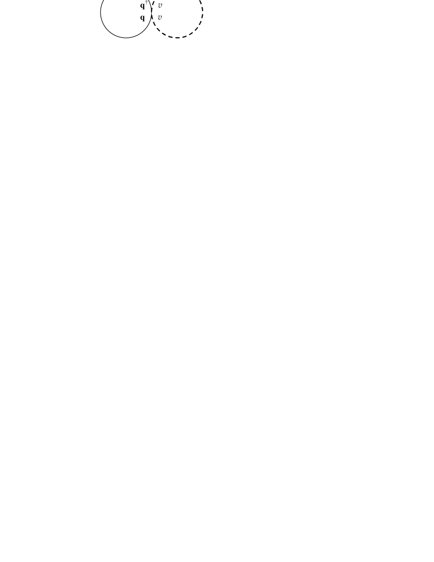
Figure 4: Two-loop supergraph IV

Finally, the supergraph in Fig. 4 leads to the following contribution

$$\Gamma_{\rm IV} = -{{\rm i}\over 16}\int{\rm d}^{8}z\int{\rm d}^{8}z^{\prime}\,\delta^{8}(z-z^{\prime})\,\langle v^{\mu}(z)\,v^{\nu}(z^{\prime})\rangle$$ (3.21)

$$\times {\rm tr}\left\{T_{\mu}\,T_{\nu}\,{\bar{\cal D}}^{2}{\cal D}^{\prime 2}G^{({\rm R})}(z,z^{\prime})\right\}~{}.$$

4 Exact superpropagators

For computing quantum corrections of the form (1.2), it is sufficient to consider a very special type of background field configuration specified by the constraint

$${\cal D}_{\alpha}{\cal W}_{\beta}=0~{}.$$ (4.1)

This is the simplest representative of background vector multiplets for which all Feynman superpropagators are known exactly [1, 2].

For the Green’s function $G\equiv G^{({\rm R})}$, we introduce the Fock-Schwinger proper-time representation

$$G(z,z^{\prime})={\rm i}\int\limits_{0}^{\infty}{\rm d}s\,K(z,z^{\prime}|s)\,{\rm e}^{-{\rm i}(|{\cal M}|^{2}-{\rm i}\varepsilon)s}~{},\qquad\varepsilon\to+0~{}.$$ (4.2)

The corresponding heat kernel reads

$$K(z,z^{\prime}|s)=-\frac{\rm i}{(4\pi s)^{2}}\,{\rm e}^{{\rm i}\rho^{2}/4s}\,\delta^{2}(\zeta-{\rm i}s\,{\cal W})\,\delta^{2}({\bar{\zeta}}+{\rm i}s\,{\bar{\cal W}})\,I(z,z^{\prime})~{},$$ (4.3)

where the supersymmetric two-point function $\zeta^{A}(z,z^{\prime})=-\zeta^{A}(z^{\prime},z)=(\rho^{a},\zeta^{\alpha},{\bar{\zeta}}_{\dot{\alpha}})$ is defined as follows:

$$\rho^{a}=(x-x^{\prime})^{a}-{\rm i}(\theta-\theta^{\prime})\sigma^{a}{\bar{\theta}}^{\prime}+{\rm i}\theta^{\prime}\sigma^{a}({\bar{\theta}}-{\bar{\theta}}^{\prime})~{},\quad\zeta^{\alpha}=(\theta-\theta^{\prime})^{\alpha}~{},\quad{\bar{\zeta}}_{\dot{\alpha}}=({\bar{\theta}}-{\bar{\theta}}^{\prime})_{\dot{\alpha}}~{}.$$ (4.4)

The parallel displacement propagator, $I(z,z^{\prime})$, is uniquely specified by the following requirements:
(i) the gauge transformation law

$$I(z,z^{\prime})~{}\to~{}{\rm e}^{{\rm i}\tau(z)}\,I(z,z^{\prime})\,{\rm e}^{-{\rm i}\tau(z^{\prime})}~{}$$ (4.5)

with respect to a gauge ($\tau$-frame) transformation of the covariant derivatives

$${\cal D}_{A}~{}\to~{}{\rm e}^{{\rm i}\tau(z)}\,{\cal D}_{A}\,{\rm e}^{-{\rm i}\tau(z)}~{},\qquad\tau^{\dagger}=\tau~{},$$ (4.6)

with the gauge parameter $\tau(z)$ being arbitrary modulo the reality condition imposed;
(ii) the equation

$$\zeta^{A}{\cal D}_{A}\,I(z,z^{\prime})=\zeta^{A}\Big{(}D_{A}+{\rm i}\,\Gamma_{A}(z)\Big{)}I(z,z^{\prime})=0~{};$$ (4.7)

(iii) the boundary condition

$$I(z,z)={\bf 1}~{}.$$ (4.8)

These imply the important relation

$$I(z,z^{\prime})\,I(z^{\prime},z)={\bf 1}~{},$$ (4.9)

as well as

$$\zeta^{A}{\cal D}^{\prime}_{A}\,I(z,z^{\prime})=\zeta^{A}\Big{(}D^{\prime}_{A}\,I(z,z^{\prime})-{\rm i}\,I(z,z^{\prime})\,\Gamma_{A}(z^{\prime})\Big{)}=0~{}.$$ (4.10)

For the background (4.1), the parallel displacement propagator is completely specified by the properties:

$$I(z^{\prime},z)\,{\cal D}_{\alpha{\dot{\alpha}}}I(z,z^{\prime}) = -{\rm i}(\zeta_{\alpha}\bar{{\cal W}}_{{\dot{\alpha}}}+{\cal W}_{\alpha}\,\bar{\zeta}_{{\dot{\alpha}}})~{},$$

$$I(z^{\prime},z)\,{\cal D}_{\alpha}I(z,z^{\prime}) = -\frac{{\rm i}}{2}\,\rho_{\alpha{\dot{\alpha}}}\bar{{\cal W}}^{{\dot{\alpha}}}+\frac{1}{3}(\zeta_{\alpha}\bar{\zeta}\bar{{\cal W}}+\bar{\zeta}^{2}{\cal W}_{\alpha})~{},$$ (4.11)

$$I(z^{\prime},z)\,{\bar{\cal D}}_{{\dot{\alpha}}}I(z,z^{\prime}) = -\frac{{\rm i}}{2}\,\rho_{\alpha{\dot{\alpha}}}{\cal W}^{\alpha}-\frac{1}{3}({\bar{\zeta}}_{\dot{\alpha}}\zeta{\cal W}+\zeta^{2}{\bar{\cal W}}_{\dot{\alpha}})~{}.$$

The heat kernel corresponding to the chiral Green’s function $G_{+}$ (2.29) is

$$K_{+}(z,z^{\prime}|s) = -{1\over 4}{\bar{\cal D}}^{2}K(z,z^{\prime}|s)$$ (4.12)

$$= -\frac{\rm i}{(4\pi s)^{2}}\,{\rm e}^{{\rm i}\rho^{2}/4s}\,\delta^{2}(\zeta-{\rm i}s\,{\cal W})\,{\rm e}^{\frac{{\rm i}}{6}s\,{\cal W}^{2}\,({\bar{\zeta}}+{\rm i}s\,{\bar{\cal W}})^{2}}\,I(z,z^{\prime})~{}.$$

It is an instructive exercise to check, using the properties of the parallel displacement propagator, that $K_{+}(z,z^{\prime}|s)$ is covariantly chiral in both arguments.

The supersymmetric theories that we are going to study below are free of ultraviolet divergences. This does not mean that individual (say, two-loop) supergraphs are all finite; only their sum, at any loop order, has to be finite. To deal with UV divergent supergraphs, we will adopt supersymmetric dimensional regularization via dimensional reduction [15]. All manipulations with the gauge covariant derivatives (D-algebra) have to be completed in four dimensions. At a final stage, the bosonic part of the heat kernel (4.3) is to be continued to $d$ dimensions using the prescription

$$\frac{\rm i}{(4\pi{\rm i}s)^{2}}\,{\rm e}^{{\rm i}\rho^{2}/4s}\quad\longrightarrow\quad\frac{\rm i}{(4\pi{\rm i}s)^{d/2}}\,{\rm e}^{{\rm i}\rho^{2}/4s}~{},\qquad\quad d=4-\varepsilon~{}.$$ (4.13)

It is assumed that loop space-time integrals are done in $d$ dimensions, using the following integration rules:

$$\frac{\rm i}{(4\pi{\rm i})^{d/2}}\int{\rm d}^{d}\rho\,{\rm e}^{{\rm i}C\rho^{2}/4} = C^{-d/2}~{},$$

$$\frac{\rm i}{(4\pi{\rm i})^{d/2}}\int{\rm d}^{d}\rho\,\rho_{a}\rho_{b}\,{\rm e}^{{\rm i}C\rho^{2}/4} = 2\,{\rm i}\,\eta_{ab}\,C^{-(d/2+1)}~{},$$ (4.14)

with $C$ a positive parameter.

5 $SU(N)$ SYM with $2N$ hypermultiplets in the fundamental

From now on, we choose the gauge group to be $SU(N)$. Lower-case Latin letters from the middle of the alphabet, $i,j,\dots$, will be used to denote matrix elements in the fundamental, with the convention $i=0,1,\dots,N-1\equiv 0,\underline{i}$. We choose a Cartan-Weyl basis to consist of the elements:

$$H_{I}=\{H_{0},H_{\underline{I}}\}~{},\quad\underline{I}=1,\dots,N-2~{},\qquad\quad E_{ij}~{},\quad i\neq j~{}.$$ (5.1)

The basis elements in the fundamental representation are defined similarly to [18],

$$(E_{ij})_{kl} = \delta_{ik}\,\delta_{jl}~{},$$

$$(H_{I})_{kl} = \frac{1}{\sqrt{(N-I)(N-I-1)}}\Big{\{}(N-I)\,\delta_{kI}\,\delta_{lI}-\sum\limits_{i=I}^{N-1}\delta_{ki}\,\delta_{li}\Big{\}}~{},$$ (5.2)

and are characterized by the properties

$${\rm tr}_{\rm F}(H_{I}\,H_{J})=\delta_{IJ}~{},\qquad{\rm tr}_{\rm F}(E_{ij}\,E_{kl})=\delta_{il}\,\delta_{jk}~{},\qquad{\rm tr}_{\rm F}(H_{I}\,E_{kl})=0~{}.$$ (5.3)

The ${\cal N}=2$ background vector multiplet is chosen to be

$$\Phi=\phi\,H_{0}~{},\qquad{\cal W}_{\alpha}=W_{\alpha}\,H_{0}~{},$$ (5.4)

Its characteristic feature is that it leaves the subgroup $U(1)\times SU(N-1)\subset SU(N)$ unbroken, where $U(1)$ is associated with $H_{0}$ and $SU(N-1)$ is generated by $\{H_{\underline{I}},\,E_{\underline{i}\underline{j}}\}$. In evaluating the supergraphs, we consider $\phi$ and $W_{\alpha}$ to be constant. This suffices for our purposes.

The mass matrix is

$$|{\cal M}|^{2}={\bar{\phi}}\phi\,(H_{0})^{2}~{},$$ (5.5)

and therefore a superfield’s mass is determined by its $U(1)$ charge with respect to $H_{0}$. With the notation

$$e_{\rm f}=\sqrt{{N-1\over N}}={1\over e_{\rm a}}~{},$$ (5.6)

the $U(1)$ charges of all quantum superfields are given in the table.

superfield	$q_{0}$	$q_{\underline{i}}$	$\tilde{q}_{0}$	$\tilde{q}_{\underline{i}}$	$v^{0\,\underline{i}}$	$v^{I}$	$v^{\underline{i}\,\underline{j}}$
$U(1)$ charge	$e_{\rm f}$	$e_{\rm f}-e_{\rm a}$	$-e_{\rm f}$	$e_{\rm a}-e_{\rm f}$	$e_{\rm a}$	0	0

Table 1: $U(1)$ charges of superfields

As can be seen, all fundamental hypermultiplet superfields are massive. For the adjoint superfields

$$v=v^{I}\,H_{I}+v^{ij}\,E_{ij}\equiv v^{\mu}\,T_{\mu}~{},\qquad i\neq j~{},$$ (5.7)

there are $2(N-1)$ massive superfields ($v^{0\underline{i}}$ and their conjugates $v^{\underline{i}0}$), while the remaining $(N-1)^{2}$ superfields, $v^{I}$ and $v^{\underline{i}\,\underline{j}}$, are free massless. This follows from the identity

$$[H_{0},E_{ij}]~{}=~{}\sqrt{N\over N-1}\,\Big{(}\delta_{0i}\,E_{0j}-\delta_{0j}\,E_{i0}\Big{)}~{}.$$ (5.8)

Let us denote by ${\bf G}^{(e)}(z,z^{\prime})$ the Green’s function (2.23) in the special case when the gauge group is $U(1)$ generated by $H_{0}$, and the quantum superfield $\Sigma$ in (2.21) carries $U(1)$ charge $e$, $H_{0}\,\Sigma=e\,\Sigma$ (in particular, the mass matrix is $|{\cal M}|^{2}=e^{2}\,{\bar{\phi}}\phi$). The Green’s function has the proper-time representation

$${\bf G}^{(e)}(z,z^{\prime})={\rm i}\int\limits_{0}^{\infty}{\rm d}s\,{\bf K}^{(e)}(z,z^{\prime}|s)\,{\rm e}^{-{\rm i}(e^{2}{\bar{\phi}}\phi-{\rm i}\varepsilon)s}~{},\qquad\varepsilon\to+0~{},$$ (5.9)

where the heat kernel is

$${\bf K}^{(e)}(z,z^{\prime}|s)=-\frac{\rm i}{(4\pi s)^{2}}\,{\rm e}^{{\rm i}\rho^{2}/4s}\,\delta^{2}(\zeta-{\rm i}es\,W)\,\delta^{2}({\bar{\zeta}}+{\rm i}es\,{\bar{W}})\,I^{(e)}(z,z^{\prime})~{}.$$ (5.10)

For the ${\cal N}=2$ background vector multiplet chosen, all the Feynman propagators are expressed via such $U(1)$ Green’s functions.

In the remainder of this section, we specialize to the case of ${\cal N}=2$ SYM with $2N$ hypermultiplets in the fundamental representation of $SU(N)$. This theory is finite since the finiteness condition (2.6) is satisfied due to the well-known $SU(N)$ identity

$${\rm tr}_{\rm Ad}\,\Psi^{2}~{}=~{}2N\,{\rm tr}_{\rm F}\,\Psi^{2}~{},\qquad\quad\Psi\in sl(N)~{}.$$ (5.11)

5.1 Evaluation of $\Gamma_{\rm I+II}$

We now turn to evaluating $\Gamma_{\rm I+II}$. In accordance with (3.18), it is necessary to analyze the expression

$$2N\,\langle v^{\mu}(z)\,v^{\nu}(z^{\prime})\rangle {\rm tr}_{\rm F} \left\{T_{\mu}\Big{(}[{\bar{\cal D}}^{2},{\cal D}^{2}]\,G^{({\rm F})}(z,z^{\prime})\Big{)}\,T_{\nu}[{\bar{\cal D}}^{\prime 2},{\cal D}^{\prime 2}]\,G^{({\rm F})}(z^{\prime},z)\right\}$$

$$=2N\sum\limits_{I}\langle v^{I}(z)\,v^{I}(z^{\prime})\rangle {\rm tr}_{\rm F} \left\{H_{I}\Big{(}[{\bar{\cal D}}^{2},{\cal D}^{2}]\,G^{({\rm F})}(z,z^{\prime})\Big{)}\,H_{I}[{\bar{\cal D}}^{\prime 2},{\cal D}^{\prime 2}]\,G^{({\rm F})}(z^{\prime},z)\right\}$$ (5.12)

$$+2N\sum\limits_{i\neq j}\langle v^{ij}(z)\,v^{ji}(z^{\prime})\rangle {\rm tr}_{\rm F} \left\{E_{ij}\Big{(}[{\bar{\cal D}}^{2},{\cal D}^{2}]\,G^{({\rm F})}(z,z^{\prime})\Big{)}\,E_{ji}[{\bar{\cal D}}^{\prime 2},{\cal D}^{\prime 2}]\,G^{({\rm F})}(z^{\prime},z)\right\}~{},$$

where the factor $2N$ relates to the presence of $2N$ hypermultiplets. The expression in the second line can be simplified on the basis of the following observations: (i) the propagator $G^{({\rm F})}$ is diagonal; (ii) the massless adjoint propagators are identical,

$$\langle v^{I}(z)\,v^{I}(z^{\prime})\rangle=\langle v^{\underline{i}\,\underline{j}}(z)\,v^{\underline{j}\,\underline{i}}(z^{\prime})\rangle={\rm i}\,g^{2}\,{\bf G}^{(0)}(z,z^{\prime})~{}.$$ (5.13)

with ${\bf G}^{(0)}(z,z^{\prime})$ the free massless Green’s function. Then, the second line of (5.12) becomes

$$2{\rm i}N\,g^{2}\,{\bf G}^{(0)}(z,z^{\prime})\,\sum\limits_{I}{\rm tr}_{\rm F}\left\{(H_{I})^{2}\Big{(}[{\bar{\cal D}}^{2},{\cal D}^{2}]\,G^{({\rm F})}(z,z^{\prime})\Big{)}\,[{\bar{\cal D}}^{\prime 2},{\cal D}^{\prime 2}]\,G^{({\rm F})}(z^{\prime},z)\right\}~{}.$$ (5.14)

In the fundamental representation of $SU(N)$,

$$\sum\limits_{I}(H^{({\rm F})}_{I})^{2}~{}=~{}{{N-1}\over N}\,{\bf 1}~{}.$$ (5.15)

This gives

$$2N\sum\limits_{I}\langle v^{I}(z)\,v^{I}(z^{\prime})\rangle{\rm tr}_{\rm F}\left\{H_{I}\Big{(}[{\bar{\cal D}}^{2},{\cal D}^{2}]\,G^{({\rm F})}(z,z^{\prime})\Big{)}\,H_{I}[{\bar{\cal D}}^{\prime 2},{\cal D}^{\prime 2}]\,G^{({\rm F})}(z^{\prime},z)\right\}$$

$$= 2{\rm i}\,(N-1)\,g^{2}\,{\bf G}^{(0)}(z,z^{\prime})\,\Big{\{}\Big{(}[{\bar{\cal D}}^{2},{\cal D}^{2}]\,{\bf G}^{(e_{\rm f})}(z,z^{\prime})\Big{)}\,[{\bar{\cal D}}^{\prime 2},{\cal D}^{\prime 2}]\,{\bf G}^{(e_{\rm f})}(z^{\prime},z)$$

$$\qquad\qquad+~{}(N-1)\Big{(}[{\bar{\cal D}}^{2},{\cal D}^{2}]\,{\bf G}^{(e_{\rm f}-e_{\rm a})}(z,z^{\prime})\Big{)}\,[{\bar{\cal D}}^{\prime 2},{\cal D}^{\prime 2}]\,{\bf G}^{(e_{\rm f}-e_{\rm a})}(z^{\prime},z)\Big{\}}~{}.$$

To transform the expression in the third line of (5.12), we notice

$${\rm tr}_{\rm F}\left\{E_{ij}\Big{(}[{\bar{\cal D}}^{2},{\cal D}^{2}]\,G^{({\rm F})}(z,z^{\prime})\Big{)}\,E_{ji}[{\bar{\cal D}}^{\prime 2},{\cal D}^{\prime 2}]\,G^{({\rm F})}(z^{\prime},z)\right\}$$

$$\quad=\Big{(}[{\bar{\cal D}}^{2},{\cal D}^{2}]\,G^{({\rm F})}(z,z^{\prime})\Big{)}_{jj}\,\Big{(}[{\bar{\cal D}}^{\prime 2},{\cal D}^{\prime 2}]\,G^{({\rm F})}(z^{\prime},z)\Big{)}_{ii}~{},$$ (5.17)

as immediately follows from the definition of $E_{ij}$. This leads to

$$\sum\limits_{i\neq j}\langle v^{ij}(z)\,v^{ji}(z^{\prime})\rangle{\rm tr}_{\rm F}\left\{E_{ij}\Big{(}[{\bar{\cal D}}^{2},{\cal D}^{2}]\,G^{({\rm F})}(z,z^{\prime})\Big{)}\,E_{ji}[{\bar{\cal D}}^{\prime 2},{\cal D}^{\prime 2}]\,G^{({\rm F})}(z^{\prime},z)\right\}$$

$$= {\rm i}\,(N-1)g^{2}\,{\bf G}^{(e_{\rm a})}(z,z^{\prime})\,\Big{(}[{\bar{\cal D}}^{2},{\cal D}^{2}]\,{\bf G}^{(e_{\rm f}-e_{\rm a})}(z,z^{\prime})\Big{)}\,[{\bar{\cal D}}^{\prime 2},{\cal D}^{\prime 2}]\,{\bf G}^{(e_{\rm f})}(z^{\prime},z)~{}+~{}(z\leftrightarrow z^{\prime})$$

$$+{\rm i}\,(N-1)(N-2)g^{2}\,{\bf G}^{(0)}(z,z^{\prime})\,\Big{(}[{\bar{\cal D}}^{2},{\cal D}^{2}]\,{\bf G}^{(e_{\rm f}-e_{\rm a})}(z,z^{\prime})\Big{)}\,[{\bar{\cal D}}^{\prime 2},{\cal D}^{\prime 2}]\,{\bf G}^{(e_{\rm f}-e_{\rm a})}(z^{\prime},z)~{}.$$

As should be clear from the above consideration, the evaluation of $\Gamma_{\rm I+II}$ amounts to computing a functional of the form

$$\int{\rm d}^{8}z\int{\rm d}^{8}z^{\prime}\,{\bf G}^{(e_{1})}(z,z^{\prime})\,\Big{(}[{\bar{\cal D}}^{2},{\cal D}^{2}]\,{\bf G}^{(e_{2})}(z,z^{\prime})\Big{)}\,[{\bar{\cal D}}^{\prime 2},{\cal D}^{\prime 2}]\,{\bf G}^{(e_{1}+e_{2})}(z^{\prime},z)~{},$$ (5.19)

for some charges $e_{1}$ and $e_{2}$. For all the Green’s functions, we introduce the proper-time representation (5.9). Due to the explicit structure of the heat kernel, eq. (5.10), the first multiplier in (5.19) contains a Grassmann delta-function,

$$\delta^{2}(\zeta-{\rm i}e_{1}s\,W)\,\delta^{2}({\bar{\zeta}}+{\rm i}e_{1}s\,{\bar{W}})~{},$$

which allows us to do the integral over $\theta^{\prime}$. Next, the second and third multipliers in (5.19) can be evaluated (in $d$ dimensions) as follows:

$$\frac{1}{16}[{\bar{\cal D}}^{2},{\cal D}^{2}]\,{\bf K}^{(e)}(z,z^{\prime}|s) \approx \phantom{-}\frac{\rm i}{(4\pi s)^{2}}\,{\rho^{\alpha{\dot{\alpha}}}\over s}(\zeta-{\rm i}esW)_{\alpha}(\bar{\zeta}+{\rm i}es{\bar{W}})_{\dot{\alpha}}\,{\rm e}^{{\rm i}\rho^{2}/4s}\,I^{(e)}(z,z^{\prime})$$

$$\longrightarrow -\frac{\rm i}{(4\pi{\rm i}s)^{d/2}}\,{\rho^{\alpha{\dot{\alpha}}}\over s}(\zeta-{\rm i}esW)_{\alpha}(\bar{\zeta}+{\rm i}es{\bar{W}})_{\dot{\alpha}}\,{\rm e}^{{\rm i}\rho^{2}/4s}\,I^{(e)}(z,z^{\prime})~{},$$

where we have omitted all terms of at least third order in the Grassmann variables $\zeta_{\alpha},\,{\bar{\zeta}}_{\dot{\alpha}}$ and $W_{\alpha},\,{\bar{W}}_{\dot{\alpha}}$ as they do not contribute to (5.19). Now, the parallel displacement propagators associated with the three Green’s functions in (5.19) simply annihilate each other. Finally , the integral over $x^{\prime}$ in (5.19) can easily be done if one first replaces the bosonic variables $\{x,x^{\prime}\}\to\{x,\rho\}$ and then applies eq. (4.14). Of special importance is the fact that the functional

$$\Psi={1\over 2^{8}}\int{\rm d}^{8}z\int{\rm d}^{8}z^{\prime}\,{\bf G}^{(0)}(z,z^{\prime})\,\Big{(}[{\bar{\cal D}}^{2},{\cal D}^{2}]\,{\bf G}^{(e)}(z,z^{\prime})\Big{)}\,[{\bar{\cal D}}^{\prime 2},{\cal D}^{\prime 2}]\,{\bf G}^{(e)}(z^{\prime},z)$$ (5.20)

is finite (so we set $d=4$) and does not depend on the charge $e$, for the background field configuration chosen,

$$\Psi = {4e^{4}\over(4\pi)^{4}}\int{\rm d}^{8}z\,W^{2}{\bar{W}}^{2}\,\int\limits_{0}^{\infty}{\rm d}s_{1}\int\limits_{0}^{\infty}{\rm d}s_{2}\int\limits_{0}^{\infty}{\rm d}s_{3}\,{\rm e}^{-e^{2}\phi{\bar{\phi}}(s_{2}+s_{3})}\,\frac{s_{1}\,s_{2}{}^{2}\,s_{3}{}^{2}}{(s_{2}s_{3}+s_{1}s_{2}+s_{1}s_{3})^{3}}$$ (5.21)

$$= {1\over 3}\,{1\over(4\pi)^{4}}\int{\rm d}^{8}z\,{W^{2}{\bar{W}}^{2}\over(\phi{\bar{\phi}})^{2}}={1\over 3}\,{1\over(4\pi)^{4}}\,\Upsilon~{},$$

see [2] for more details.

The computational scheme outlined leads to the final result:

$$\Gamma_{\rm I+II}=\frac{g^{2}}{(4\pi)^{4}}\,\Upsilon\Big{\{}{1\over 3}\,N(N-1)^{2}+8\,N(N-1)\,I_{\rm I+II}\Big{\}}~{},$$ (5.22)

where

$$I_{\rm I+II}=\int\limits_{0}^{\infty}{\rm d}s_{1}{\rm d}s_{2}{\rm d}s_{3}\,{\rm e}^{-[{\rm e}_{\rm a}^{2}s_{1}+({\rm e}_{\rm a}-{\rm e}_{\rm f})^{2}s_{3}+{\rm e}_{\rm f}^{2}s_{2}]}\,\frac{s_{1}[{\rm e}_{\rm a}s_{1}+({\rm e}_{\rm a}-{\rm e}_{\rm f})s_{3}]^{2}[{\rm e}_{\rm a}s_{1}+{\rm e}_{\rm f}s_{2}]^{2}}{[s_{2}s_{3}+s_{1}s_{2}+s_{1}s_{3}]^{d/2+1}}$$ (5.23)

is a divergent integral in the limit $\varepsilon=4-d\to 0$.

To isolate the divergence in (5.23), we first rescale the integral

$$I_{\rm I+II} = {(N-1)^{4}\over N^{2}}\int\limits_{0}^{\infty}{\rm d}t_{1}{\rm d}t_{2}{\rm d}t_{3}\,{\rm e}^{-[t_{1}+t_{2}+t_{3}]}\,\frac{t_{1}[t_{1}+Nt_{3}]^{2}[t_{1}+{N\over N-1}t_{2}]^{2}}{[t_{1}t_{2}+(N-1)^{2}t_{1}t_{3}+N^{2}t_{2}t_{3}]^{d/2+1}}~{}.$$ (5.24)

Now, it is advantageous to introduce new variables [19]:

$$t_{1}=s\,t\,u~{},\qquad t_{2}=s\,t\,(1-u)~{},\qquad t_{3}=s\,(1-t)~{},$$ (5.25)

with the important properties $s=t_{1}+t_{2}+t_{3}$, $s\,t=t_{1}+t_{2}$ and

$$\int\limits_{0}^{\infty}{\rm d}t_{1}\int\limits_{0}^{\infty}{\rm d}t_{2}\int\limits_{0}^{\infty}{\rm d}t_{3}\cdots~{}=~{}\int\limits_{0}^{\infty}{\rm d}s\int\limits_{0}^{1}{\rm d}t\int\limits_{0}^{1}{\rm d}u\,s^{2}\,t\cdots$$ (5.26)

The integral over $s$ factorizes and it is convergent,

$$\int\limits_{0}^{\infty}{\rm d}s\,s^{5-d}\,{\rm e}^{-s}=1+O(\varepsilon)~{}.$$ (5.27)

As a result , we obtain

$$I_{\rm I+II} = \left({N-1\over N}\right)^{2}\int\limits_{0}^{1}{\rm d}t\int\limits_{0}^{1}{\rm d}u\frac{t^{3-d/2}u[N-u]^{2}[N-t(N-u)]^{2}}{[(N-u)^{2}(1-t)+u(1-u)]^{d/2+1}}~{}+~{}{\rm finite}~{}.$$ (5.28)

The divergent part of $I_{\rm I+II}$ turns out to be

$$(I_{\rm I+II})_{\rm div}=\left(-1+4\,{N-1\over N^{2}}\right)\,{1\over\varepsilon}~{}.$$ (5.29)

5.2 Evaluation of $\Gamma_{\rm III}$

The evaluation of $\Gamma_{\rm III}$ is very similar to that of $\Gamma_{\rm I+II}$ just described. Therefore, we simply give the final result:

$$\Gamma_{\rm III}=\frac{g^{2}}{(4\pi)^{4}}\,\Upsilon\Big{\{}{2\over 3}\,N(N-1)^{2}-4\,(N-1)\,I_{\rm III}\Big{\}}~{},$$ (5.30)

where

$$I_{\rm III}=\int\limits_{0}^{\infty}{\rm d}s_{1}{\rm d}s_{2}{\rm d}s_{3}\,{\rm e}^{-[{\rm e}_{\rm a}^{2}s_{1}+({\rm e}_{\rm a}-{\rm e}_{\rm f})^{2}s_{3}+{\rm e}_{\rm f}^{2}s_{2}]}\,\frac{[{\rm e}_{\rm a}s_{1}+({\rm e}_{\rm a}-{\rm e}_{\rm f})s_{3}]^{2}[{\rm e}_{\rm a}s_{1}+{\rm e}_{\rm f}s_{2}]^{2}}{[s_{2}s_{3}+s_{1}s_{2}+s_{1}s_{3}]^{d/2}}$$ (5.31)

is a divergent integral in the limit $\varepsilon=4-d\to 0$. Its divergent part proves to be

$$(I_{\rm III})_{\rm div}=4\,{N-1\over N}\,{1\over\varepsilon}~{}.$$ (5.32)

5.3 Evaluation of $\Gamma_{\rm IV}$

It remains to evaluate $\Gamma_{\rm IV}$. As is seen from its defining expression (3.21), $\Gamma_{\rm IV}$ involves a vector propagators at coincident points, $\langle v^{\mu}(z)\,v^{\nu}(z)\rangle$. The latter is non-trivial only for the massive superfields,

$$\langle v^{I}(z)\,v^{I}(z)\rangle = \langle v^{\underline{i}\underline{j}}(z)\,v^{\underline{j}\underline{i}}(z)\rangle=0~{},$$

$$\langle v^{0\underline{i}}(z)\,v^{\underline{i}0}(z)\rangle = \langle v^{\underline{i}0}(z)\,v^{0\underline{i}}(z)\rangle=-{g^{2}\over 8\pi^{2}}\left({N-1\over N}\right)\,\frac{W^{2}{\bar{W}}^{2}}{(\phi{\bar{\phi}})^{3}}~{}.$$ (5.33)

Thus, we can rewrite $\Gamma_{\rm IV}$ in the form

$$\Gamma_{\rm IV} = {{\rm i}g^{2}\over 128\pi^{2}}\left({N-1\over N}\right)\int{\rm d}^{8}z\frac{W^{2}{\bar{W}}^{2}}{(\phi{\bar{\phi}})^{3}}\,{\rm tr}\left\{\{E_{0\underline{i}},E_{\underline{i}0}\}\,{\bar{\cal D}}^{2}{\cal D}^{\prime 2}G^{({\rm R})}(z,z^{\prime})\Big{|}_{z^{\prime}=z}\right\}~{}.$$ (5.34)

In the superconformal theory under consideration, the quantum correction (5.34) is

$$\Gamma_{\rm IV} = {{\rm i}g^{2}\over 64\pi^{2}}(N-1)\int{\rm d}^{8}z\frac{W^{2}{\bar{W}}^{2}}{(\phi{\bar{\phi}})^{3}}\,{\rm tr}_{\rm F}\left\{\{E_{0\underline{i}},E_{\underline{i}0}\}\,{\bar{\cal D}}^{2}{\cal D}^{\prime 2}G^{({\rm F})}(z,z^{\prime})\Big{|}_{z^{\prime}=z}\right\}~{}.$$ (5.35)

Its direct evaluation gives

$$\Gamma_{\rm IV}=-4\frac{g^{2}}{(4\pi)^{4}}\,\Upsilon\,(N-1)\Big{\{}N-2\,{N-1\over N}\Big{\}}\,I_{\rm IV}~{},$$ (5.36)

where

$$I_{\rm IV}=\int\limits_{0}^{\infty}{\rm d}s\,s^{-d/2}\,{\rm e}^{-s}$$ (5.37)

is a a divergent integral in the limit $\varepsilon=4-d\to 0$,

$$(I_{\rm IV})_{\rm div}=-{2\over\varepsilon}~{}.$$ (5.38)

It is easy to check that

$$\Big{(}\Gamma_{\rm I+II}+\Gamma_{\rm III}+\Gamma_{\rm IV}\Big{)}_{\rm div}=0~{},$$ (5.39)

consistent with the finiteness of the theory.

6 ${\cal N}=4$ SYM

We now turn to evaluating to the two-loop supergraphs with quantum hypermultiplets in the ${\cal N}=4$ super Yang-Mills theory which is simply ${\cal N}=2$ SYM with a single hypermultiplet in the adjoint.

6.1 Evaluation of $\Gamma_{\rm I+II}$

We start by analyzing $\Gamma_{\rm I+II}$ in the case of the adjoint representation. According to (3.18), we have to compute

$$\langle v^{\mu}\,v^{\prime\nu}\rangle{\rm tr}_{\rm Ad}\left\{T_{\mu}\hat{G}\,T_{\nu}\,\hat{G}^{\prime}\right\}$$ (6.1)

where we have introduced the following condensed notation:

$$\langle v^{\mu}\,v^{\prime\nu}\rangle=\langle v^{\mu}(z)\,v^{\nu}(z^{\prime})\rangle~{},\quad\hat{G}=[{\bar{\cal D}}^{2},{\cal D}^{2}]\,G^{({\rm Ad})}(z,z^{\prime})~{},\quad\hat{G}^{\prime}=[{\bar{\cal D}}^{\prime 2},{\cal D}^{\prime 2}]\,G^{({\rm Ad})}(z^{\prime},z)~{}.$$

Relative to the basis $T_{\mu}=(H_{I},E_{0\underline{i}},E_{\underline{i}0},E_{\underline{i}\underline{j}})$, the hypermultiplet operator $\hat{G}=(\hat{G}^{\lambda}{}_{\rho})$ in (6.1) has a diagonal structure,

$$\hat{G}={\rm diag}\Big{(}\hat{{\bf G}}^{(0)}\,{\bf 1}_{N-1},~{}\hat{{\bf G}}^{(e_{\rm a})}\,{\bf 1}_{N-1},~{}\hat{{\bf G}}^{(-e_{\rm a})}\,{\bf 1}_{N-1},~{}\hat{{\bf G}}^{(0)}\,{\bf 1}_{(N-1)(N-2)}\Big{)}~{},$$ (6.2)

with the $U(1)$ charges given explicitly. The evaluation of (6.1) will be based on considerations of charge conservation. At each vertex ($z$ or $z^{\prime}$), the total charge must be zero. The possible charges in the adjoint representation are: $0,\pm e_{\rm a}$. Therefore, there are contributions to (6.1) of the two different types: (i) one line is neutral, and hence free massless, while the other two lines carry charges $\pm e_{\rm a}$; (ii) all three lines are neutral, and hence free massless. The case (ii) can safely be ignored since no dependence on the background fields is present. With such considerations in mind, we first separate the contributions to (6.1) with neutral and charged gauge field lines:

$$\sum\limits_{I}\langle v^{I}\,v^{\prime I}\rangle{\rm tr}_{\rm Ad}\left\{H_{I}\hat{G}\,H_{I}\,\hat{G}^{\prime}\right\}+\sum\limits_{\underline{i}\neq\underline{j}}\langle v^{\underline{i}\underline{j}}\,v^{\prime\underline{j}\underline{i}}\rangle{\rm tr}_{\rm Ad}\left\{E_{\underline{i}\underline{j}}\hat{G}\,E_{\underline{j}\underline{i}}\,\hat{G}^{\prime}\right\}$$ (6.3)

$$+ \sum\limits_{\underline{i}}\langle v^{0\underline{i}}\,v^{\prime\underline{i}0}\rangle{\rm tr}_{\rm Ad}\left\{E_{0\underline{i}}\hat{G}\,E_{\underline{i}0}\,\hat{G}^{\prime}\right\}+\sum\limits_{\underline{i}}\langle v^{\underline{i}0}\,v^{\prime 0\underline{i}}\rangle{\rm tr}_{\rm Ad}\left\{E_{\underline{i}0}\hat{G}\,E_{0\underline{i}}\,\hat{G}^{\prime}\right\}~{}.$$

Since the propagators $\langle v^{I}\,v^{\prime I}\rangle=\langle v^{\underline{i}\underline{j}}\,v^{\prime\underline{j}\underline{i}}\rangle={\rm i}\,g^{2}{\bf G}^{(0)}(z,z^{\prime})$ are free massless, both $\hat{G}$ and $\hat{G}^{\prime}$ in the first line of (6.3) should be charged. In the second line of (6.3), one of the $\hat{G}$ and $\hat{G}^{\prime}$ should be neutral, while the other is charged. We will analyze separately the contributions appearing in (6.3).

Let $T^{({\rm Ad})}_{\mu}$ be the matrix generators in the adjoint representation,

$$[T_{\mu},T_{\nu}]=T_{\lambda}\,(T^{({\rm Ad})}_{\mu})^{\lambda}{}_{\nu}~{}.$$ (6.4)

Since $H_{I}$, $\hat{G}$ and $\hat{G}^{\prime}$ are diagonal, the first term in (6.3) becomes

$$\sum\limits_{I}\langle v^{I}\,v^{\prime I}\rangle{\rm tr}_{\rm Ad}\left\{H_{I}\hat{G}\,H_{I}\,\hat{G}^{\prime}\right\}=\sum\limits_{I}\langle v^{I}\,v^{\prime I}\rangle{\rm tr}_{\rm Ad}\left\{(H_{I})^{2}\hat{G}\,\hat{G}^{\prime}\right\}$$ (6.5)

$$= {\rm i}\,g^{2}\,{\bf G}^{(0)}(z,z^{\prime})\Big{\{}\hat{{\bf G}}^{(e_{\rm a})}\,\hat{{\bf G}}^{\prime(e_{\rm a})}+\hat{{\bf G}}^{(-e_{\rm a})}\,\hat{{\bf G}}^{\prime(-e_{\rm a})}\Big{\}}\sum\limits_{I}\sum\limits_{\underline{i}}(H^{({\rm Ad})}_{I})^{0\underline{i}}{}_{0\underline{i}}\,(H^{({\rm Ad})}_{I})^{0\underline{i}}{}_{0\underline{i}}~{},$$

where we have used the identity

$$(H^{({\rm Ad})}_{I})^{0\underline{i}}{}_{0\underline{i}}=-(H^{({\rm Ad})}_{I})^{\underline{i}0}{}_{\underline{i}0}~{}.$$ (6.6)

The group-theoretic factor in the last expression is easy to evaluate:

$$\sum\limits_{I}\sum\limits_{\underline{i}}(H^{({\rm Ad})}_{I})^{0\underline{i}}{}_{0\underline{i}}\,(H^{({\rm Ad})}_{I})^{0\underline{i}}{}_{0\underline{i}}=2(N-1)~{}.$$ (6.7)

Let us turn to the second term in (6.3),

$$\sum\limits_{\underline{i}\neq\underline{j}}\langle v^{\underline{i}\underline{j}}\,v^{\prime\underline{j}\underline{i}}\rangle{\rm tr}_{\rm Ad}\left\{E_{\underline{i}\underline{j}}\hat{G}\,E_{\underline{j}\underline{i}}\,\hat{G}^{\prime}\right\}={\rm i}\,g^{2}\,{\bf G}^{(0)}(z,z^{\prime})\,\sum\limits_{\underline{i}\neq\underline{j}}{\rm tr}_{\rm Ad}\left\{E_{\underline{i}\underline{j}}\hat{G}\,E_{\underline{j}\underline{i}}\,\hat{G}^{\prime}\right\}~{}.$$ (6.8)

Since both the hypermultiplets must be massive and of opposite charge, for this expression we get

$${\rm i}\,g^{2}\,{\bf G}^{(0)}(z,z^{\prime})\Big{\{}\hat{{\bf G}}^{(e_{\rm a})}\,\hat{{\bf G}}^{\prime(e_{\rm a})}+\hat{{\bf G}}^{(-e_{\rm a})}\,\hat{{\bf G}}^{\prime(-e_{\rm a})}\Big{\}}\sum\limits_{\underline{i}\neq\underline{j}}\sum\limits_{\underline{k},\,\underline{l}}(E^{({\rm Ad})}_{\underline{i}\underline{j}})^{0\underline{k}}{}_{0\underline{l}}\,(E^{({\rm Ad})}_{\underline{i}\underline{j}})^{0\underline{l}}{}_{0\underline{k}}~{},$$ (6.9)

where the following identity

$$(E^{({\rm Ad})}_{\underline{i}\underline{j}})^{\underline{k}0}{}_{\underline{l}0}=-(E^{({\rm Ad})}_{\underline{i}\underline{j}})^{0\underline{l}}{}_{0\underline{k}}$$ (6.10)

has been used. The group-theoretic factor in the last expression is also easy to evaluate:

$$\sum\limits_{\underline{i}\neq\underline{j}}\sum\limits_{\underline{k},\,\underline{l}}(E^{({\rm Ad})}_{\underline{i}\underline{j}})^{0\underline{k}}{}_{0\underline{l}}\,(E^{({\rm Ad})}_{\underline{i}\underline{j}})^{0\underline{l}}{}_{0\underline{k}}=(N-1)(N-2)~{}.$$ (6.11)

As a result, the first and second terms in (6.3) lead to the following contribution

$${\rm i}\,N(N-1)\,g^{2}\,{\bf G}^{(0)}(z,z^{\prime})\Big{\{}\hat{{\bf G}}^{(e_{\rm a})}\,\hat{{\bf G}}^{\prime(e_{\rm a})}+\hat{{\bf G}}^{(-e_{\rm a})}\,\hat{{\bf G}}^{\prime(-e_{\rm a})}\Big{\}}~{}.$$ (6.12)

We now turn to the third term in (6.3). Since $\langle v^{0\underline{i}}\,v^{\prime\underline{i}0}\rangle={\rm i}\,g^{2}{\bf G}^{(e_{\rm a})}(z,z^{\prime})$ is a massive propagator of charge $+e_{\rm a}$, one of the hypermultiplet propagators must be massive of charge $-e_{\rm a}$, with the other must be free neutral.

$$\qquad\qquad\sum\limits_{\underline{i}}\langle v^{0\underline{i}}\,v^{\prime\underline{i}0}\rangle{\rm tr}_{\rm Ad}\left\{E_{0\underline{i}}\hat{G}\,E_{\underline{i}0}\,\hat{G}^{\prime}\right\}$$

$$= {\rm i}\,g^{2}\,{\bf G}^{(e_{\rm a})}(z,z^{\prime})\,\hat{{\bf G}}^{(-e_{\rm a})}\,\hat{{\bf G}}^{\prime(0)}\Bigg{\{}\sum\limits_{\underline{i},\,\underline{j}}\sum\limits_{I}(E^{({\rm Ad})}_{0\underline{i}})^{I}{}_{0\underline{j}}\,(E^{({\rm Ad})}_{\underline{i}0})^{0\underline{j}}{}_{I}+\sum\limits_{\underline{i},\,\underline{j}}\sum\limits_{\underline{k}\neq\underline{l}}(E^{({\rm Ad})}_{0\underline{i}})^{\underline{k}\underline{l}}{}_{0\underline{j}}\,(E^{({\rm Ad})}_{\underline{i}0})^{0\underline{j}}{}_{\underline{k}\underline{l}}\Bigg{\}}$$

$$+ {\rm i}\,g^{2}\,{\bf G}^{(e_{\rm a})}(z,z^{\prime})\hat{{\bf G}}^{(0)}\,\hat{{\bf G}}^{\prime(-e_{\rm a})}\Bigg{\{}\sum\limits_{\underline{i},\,\underline{j}}\sum\limits_{I}(E^{({\rm Ad})}_{0\underline{i}})^{0\underline{j}}{}_{I}\,(E^{({\rm Ad})}_{\underline{i}0})^{I}{}_{0\underline{j}}+\sum\limits_{\underline{i},\,\underline{j}}\sum\limits_{\underline{k}\neq\underline{l}}(E^{({\rm Ad})}_{0\underline{i}})^{0\underline{j}}{}_{\underline{k}\underline{l}}\,(E^{({\rm Ad})}_{\underline{i}0})^{\underline{k}\underline{l}}{}_{0\underline{j}}\Bigg{\}}~{}.$$

Using the symmetry properties of the structure constants, the group-theoretical factors here can be related to those which occur in eqs. (6.7) and (6.11):

$$\sum\limits_{\underline{i},\,\underline{j}}\sum\limits_{I}(E^{({\rm Ad})}_{0\underline{i}})^{I}{}_{0\underline{j}}\,(E^{({\rm Ad})}_{\underline{i}0})^{0\underline{j}}{}_{I} = \sum\limits_{\underline{i},\,\underline{j}}\sum\limits_{I}(E^{({\rm Ad})}_{0\underline{i}})^{0\underline{j}}{}_{I}\,(E^{({\rm Ad})}_{\underline{i}0})^{I}{}_{0\underline{j}}=2(N-1)~{},$$ (6.14)

$$\sum\limits_{\underline{i},\,\underline{j}}\sum\limits_{\underline{k}\neq\underline{l}}(E^{({\rm Ad})}_{0\underline{i}})^{\underline{k}\underline{l}}{}_{0\underline{j}}\,(E^{({\rm Ad})}_{\underline{i}0})^{0\underline{j}}{}_{\underline{k}\underline{l}} = \sum\limits_{\underline{i},\,\underline{j}}\sum\limits_{\underline{k}\neq\underline{l}}(E^{({\rm Ad})}_{0\underline{i}})^{0\underline{j}}{}_{\underline{k}\underline{l}}\,(E^{({\rm Ad})}_{\underline{i}0})^{\underline{k}\underline{l}}{}_{0\underline{j}}=(N-1)(N-2)~{}.$$

As a result, the third term in (6.3) leads to the following contribution

$${\rm i}\,N(N-1)\,g^{2}\,{\bf G}^{(e_{\rm a})}(z,z^{\prime})\,\Big{\{}\hat{{\bf G}}^{(-e_{\rm a})}\,\hat{{\bf G}}^{\prime(0)}+\hat{{\bf G}}^{(0)}\,\hat{{\bf G}}^{\prime(e_{\rm a})}\Big{\}}~{}.$$ (6.15)

On the base of the above considerations, one can readily arrive at the final expression for $\Gamma_{\rm I+II}$:

$$\Gamma_{\rm I+II}=N(N-1)\,\frac{g^{2}}{(4\pi)^{4}}\,\Upsilon\Big{\{}{1\over 3}+8\,\hat{I}_{\rm I+II}\Big{\}}~{},$$ (6.16)

where

$$\hat{I}_{\rm I+II}=\int\limits_{0}^{\infty}{\rm d}s_{1}{\rm d}s_{2}{\rm d}s_{3}\,{\rm e}^{-[s_{1}+s_{2}]}\,\frac{s_{1}^{3}[s_{1}+s_{2}]^{2}}{[s_{2}s_{3}+s_{1}s_{2}+s_{1}s_{3}]^{d/2+1}}$$ (6.17)

is a divergent integral in the limit $\varepsilon=4-d\to 0$. This integral follows from (5.23) in the limit $e_{\rm a}=e_{\rm f}=1$ or, equivalently, $N\to\infty$. Therefore, the divergent part of $\hat{I}_{\rm I+II}$ can be read off from (5.29),

$$(\hat{I}_{\rm I+II})_{\rm div}=-{1\over\varepsilon}~{}.$$ (6.18)

6.2 Evaluation of $\Gamma_{\rm III}$

The evaluation of $\Gamma_{\rm III}$ is very similar to that of $\Gamma_{\rm I+II}$ just described. Therefore, we simply give the final result:

$$\Gamma_{\rm III}={2\over 3}\,N(N-1)\,\frac{g^{2}}{(4\pi)^{4}}\,\Upsilon~{}.$$ (6.19)

No divergences are present.

6.3 Evaluation of $\Gamma_{\rm IV}$

It remains to evaluate $\Gamma_{\rm IV}$ which is determined by eq. (5.34). In supersymmetric dimensional regularization, we have

$${1\over 16}\,{\bar{\cal D}}^{2}{\cal D}^{\prime 2}{\bf G}^{(e)}(z,z^{\prime})\Big{|}_{z^{\prime}=z} = \frac{(e^{2}\,\phi{\bar{\phi}})^{d/2-1}}{(4\pi)^{d/2}}\,\int\limits_{0}^{\infty}\frac{{\rm d}s}{s^{d/2}}\,{\rm e}^{-s}~{},\qquad e\neq 0~{},$$

$${1\over 16}\,{\bar{\cal D}}^{2}{\cal D}^{\prime 2}{\bf G}^{(0)}(z,z^{\prime})\Big{|}_{z^{\prime}=z} = 0~{}.$$ (6.20)

The second relation here is actually a consequence of one of the fancy properties of dimensional regularization (see, e.g. [19])

$$\int\frac{{\rm d}^{d}p}{p^{2}}=0\quad\Longleftrightarrow\quad\int\limits_{0}^{\infty}\frac{{\rm d}s}{s^{d/2}}=0~{}.$$ (6.21)

Therefore, in the expression

$${\rm tr}_{\rm Ad}\left\{\{E_{0\underline{i}},E_{\underline{i}0}\}\,{\bar{\cal D}}^{2}{\cal D}^{\prime 2}G^{({\rm Ad})}(z,z^{\prime})\Big{|}_{z^{\prime}=z}\right\}~{},$$ (6.22)

which occurs in (5.34), we should take into account the massive modes only. This amounts to computing the following group-theoretic factor

$$\sum\limits_{\underline{i},\,\underline{j}}\left(\Big{(}\{E^{({\rm Ad})}_{0\underline{i}},E^{({\rm Ad})}_{\underline{i}0}\}\Big{)}^{0\underline{j}}{}_{0\underline{j}}+\Big{(}\{E^{({\rm Ad})}_{0\underline{i}},E^{({\rm Ad})}_{\underline{i}0}\}\Big{)}^{\underline{j}0}{}_{\underline{j}0}\right)=2N(N-1)~{}.$$ (6.23)

As a result, we obtain

$$\Gamma_{\rm IV}=-4N(N-1)\,\frac{g^{2}}{(4\pi)^{4}}\,\Upsilon\,I_{\rm IV}~{},$$ (6.24)

with $I_{\rm IV}$ given in (5.37). It is seen that the divergent parts of of $\Gamma_{\rm I+II}$ and $\Gamma_{\rm IV}$ cancel each other,

$$\Big{(}\Gamma_{\rm I+II}+\Gamma_{\rm IV}\Big{)}_{\rm div}=0~{},$$ (6.25)

consistent with the finiteness of the theory. An alternative treatment of the cancellation of divergences is given in the Appendix.

7 Discussion

As pointed out in the Introduction, the two ${\cal N}=2$ superconformal field theories with gauge group $SU(N)$ considered in this paper differ only in the hypermultiplet sector — one contains a single hypermultiplet in the adjoint representation, the other contains $2N$ hypermultiplets in the fundamental representation. If the Dine-Seiberg conjecture holds, then the two-loop $F^{4}$ contributions to the effective action must vanish in both theories. This would necessitate a cancellation of the $F^{4}$ corrections between the pure ${\cal N}=2$ SYM, ghost and hypermultiplet sectors in both theories, implying that both theories should yield identical two-loop $F^{4}$ contributions in the hypermultiplet sector.

By explicit calculation, we have found the following two-loop $F^{4}$ contributions, $\Gamma_{\rm I+II}+\Gamma_{\rm III}+\Gamma_{\rm IV}$, from the hypermultiplet sector. For the case of ${\cal N}=2$ SYM with $2N$ hypermultiplets in the fundamental:

$$\frac{g^{2}\,\Upsilon}{(4\pi)^{4}}\,\Big{\{}N(N-1)(N-2) + N(N-1)$$

$$+8N(N-1)I_{\rm I+II} - 4(N-1)I_{\rm III}-4(N-1)(N-2\,{N-1\over N})I_{\rm IV}\Big{\}}~{},$$ (7.1)

where the integrals $I_{\rm I+II},$ $I_{\rm III}$ and $I_{\rm IV}$ are given in equations (5.23), (5.31) and (5.37) respectively. For the case of ${\cal N}=4$ SYM:

$$\frac{g^{2}\,\Upsilon}{(4\pi)^{4}}\,\Big{\{}N(N-1)+8N(N-1)\,\hat{I}_{\rm I+II}-4N(N-1)\,I_{\rm IV}\Big{\}}~{},$$ (7.2)

where the integrals $\hat{I}_{\rm I+II}$ and $I_{\rm IV}$ are given in equations (6.17) and (5.37) respectively.

In the large $N$ limit, all of the integrals contained in the expressions (7.1) and (7.2) become independent of $N,$ as the charges $e_{\rm a}$ and $e_{\rm f}$ approach 1. With this observation, it is clear that these $F^{4}$ contributions have different large $N$ behaviour. The leading term in (7.1) is of order $N^{3},$ while the leading term in (7.2) is of order $N^{2}.$ This is inconsistent with the Dine-Seiberg conjecture, which would require identical leading large $N$ behaviour for the two theories.

It is instructive to examine the source of the difference in the large $N$ behaviour of the two theories, which is due to the presence of a leading $N^{3}$ contribution in the case of ${\cal N}=2$ SYM with $2N$ hypermultiplets in the fundamental. This contribution comes from the diagrams of type I, II and III in which the ${\cal N}=2$ vector multiplet propagator (that is, $\langle v\,v\rangle$ or $\langle\varphi\,\varphi^{\dagger}\rangle$) is massless and corresponds to one of the unbroken $SU(N-1)$ generators $E_{\underline{i}\underline{j}}$, and the two hypermultiplet propagators are massive with the same mass $\bar{\phi}\phi/N(N-1)$. In the large $N$ limit, these hypermultiplets become massless and decouple from the background (as their $U(1)$ charges, $\pm 1/\sqrt{N(N-1))}$, vanish), and so one might at first sight expect these diagrams not to contribute terms proportional to $\Upsilon$ in the large $N$ limit. However, the situation is more subtle, because they really decouple only for $N=\infty$. The point is that the magnitude of the $U(1)$ charge on each of the hypermultiplet lines is the same. Since all charge dependence occurs in the form $eW$ or $e\phi,$ it cancels out of the terms proportional to $W^{2}\bar{W}^{2}/(\phi\bar{\phi})^{2}$, see eqs. (5.20) and (5.21). As a result, the contribution from these diagrams survives in the large $N$ limit. There is a combinatoric factor of $2N(N-1)(N-2),$ as there are $2N$ hypermultiplets and $(N-1)(N-2)$ massless vectors $v^{\underline{i}\underline{j}}.$

There remains a (pretty solid) hope that the Dine-Seiberg conjecture holds, at least in the large $N$ limit, for those ${\cal N}=2$ superconformal theories which possess supergravity duals, in particular: (i) ${\cal N}=4$ SYM; (ii) $USp(2N)$ gauge theory with a traceless antisymmetric hypermultiplet and four fundamental hypermultiplets [20]; (iii) quiver gauge theories [21]. This is based upon the AdS/CFT correspondence. Maximal supersymmetry should also play a crucial role in the case of ${\cal N}=4$ SYM. Otherwise one would be forced to re-consider numerous conclusions drawn on the basis of this conjecture, for instance, in [22, 23]. Explicit two-loop calculations of $F^{4}$ corrections in such theories are therefore extremely desirable and can be carried out using the techniques developed in the present paper in conjunction with some ideas given in [23].

Acknowledgements:
We are grateful to Joseph Buchbinder, Jim Gates and Arkady Tseytlin for comments. This work is supported in part by the Australian Research Council and UWA research grants.

Appendix A Cancellation of divergences

To handle ill-defined two-loop integrals, we employed supersymmetric regularization via dimensional reduction. Its use allowed us, in a safe yet simple way, to make sure that no divergences are present. On the other hand, the absence of divergences indicates that there should exist a manifestly finite form for the effective action directly in four space-time dimensions. Here we elaborate on such a form in the case of ${\cal N}=4$ SYM.

The second and third terms in the two-loop contribution (7.2) contain the proper-time integrals $\hat{I}_{\rm I+II}$ (6.17) and $I_{\rm IV}$ (5.37), each of which diverges in $d=4$. Nevertheless, let us try to evaluate the joint contribution coming from the second and third terms in (7.2) in $d=4$. Since we no longer use supersymmetric dimensional regularization, the integral $I_{\rm IV}$ has to be modified as follows

$$I_{\rm IV}\quad\longrightarrow\quad\hat{I}_{\rm IV}=\int\limits_{0}^{\infty}{{\rm d}s\over s^{d/2}}\,{\rm e}^{-s}+\int\limits_{0}^{\infty}{{\rm d}s\over s^{d/2}}~{}.$$ (A.1)

The second term here is generated by those supergraphs of type IV which involve the structure in the second line of (6.20). This term cannot be ignored anymore, since the identity (6.21) holds only in the framework of supersymmetric dimensional regularization. The sum of divergent integrals is

$$\Big{(}2\hat{I}_{\rm I+II}-\hat{I}_{\rm IV}\Big{)}\Big{|}_{d=4}=2\int\limits_{0}^{\infty}{\rm d}s\,{\rm d}t\,{\rm d}u\,\frac{t^{3}\,(s+t)^{2}}{(st+su+tu)^{3}}\,{\rm e}^{-(s+t)}-\int\limits_{0}^{\infty}{{\rm d}s\over s^{2}}\,{\rm e}^{-s}-\int\limits_{0}^{\infty}{{\rm d}s\over s^{2}}~{}.$$ (A.2)

In the first term on the right, one can easily do the $u$-integral:

$$\int\limits_{0}^{\infty}{\rm d}s\,{\rm d}t\,{\rm d}u\,\frac{t^{3}\,(s+t)^{2}}{(st+su+tu)^{3}}\,{\rm e}^{-(s+t)} = \frac{1}{2}\int\limits_{0}^{\infty}{\rm d}s\,{\rm d}t\,\frac{t\,(s+t)}{s^{2}}\,{\rm e}^{-(s+t)}$$

$$=\frac{1}{2}\int\limits_{0}^{\infty}{\rm d}t\,t\,{\rm e}^{-t}\int\limits_{0}^{\infty}{{\rm d}s\over s}\,{\rm e}^{-s} + \frac{1}{2}\int\limits_{0}^{\infty}{\rm d}t\,t^{2}\,{\rm e}^{-t}\int\limits_{0}^{\infty}{{\rm d}s\over s^{2}}\,{\rm e}^{-s}~{}.$$ (A.3)

As a result, one gets

$$\Big{(}2\hat{I}_{\rm I+II}-\hat{I}_{\rm IV}\Big{)}\Big{|}_{d=4}=\int\limits_{0}^{\infty}{\rm d}s\,{{\rm d}\over{\rm d}s}\,\left\{\frac{1}{s}\,(1-{\rm e}^{-s})\right\}=-1~{}.$$ (A.4)

This shows that the second and third terms in (7.2) provide a finite contribution to the effective action.

References

• [1] S. M. Kuzenko and I. N. McArthur, “On the background field method beyond one loop: A manifestly covariant derivative expansion in super Yang-Mills theories,” JHEP 0305 (2003) 015 [arXiv:hep-th/0302205].
• [2] S. M. Kuzenko and I. N. McArthur, “Low-energy dynamics in N = 2 super QED: Two-loop approximation,” JHEP 0310 (2003) 029 [arXiv:hep-th/0308136].
• [3] I. L. Buchbinder, S. M. Kuzenko and B. A. Ovrut, “On the D = 4, N = 2 non-renormalization theorem,” Phys. Lett. B 433 (1998) 335 [arXiv:hep-th/9710142].
• [4] I. L. Buchbinder, E. I. Buchbinder, S. M. Kuzenko and B. A. Ovrut, “The background field method for N = 2 super Yang-Mills theories in harmonic superspace,” Phys. Lett. B 417 (1998) 61 [arXiv:hep-th/9704214].
• [5] M. Dine and N. Seiberg, “Comments on higher derivative operators in some SUSY field theories,” Phys. Lett. B 409 (1997) 239 [arXiv:hep-th/9705057].
• [6] B. de Wit, M. T. Grisaru and M. Roček, “Nonholomorphic corrections to the one-loop N=2 super Yang-Mills action,” Phys. Lett. B 374 (1996) 297 [arXiv:hep-th/9601115].
• [7] M. Henningson, “Extended superspace, higher derivatives and SL(2,Z) duality,” Nucl. Phys. B 458 (1996) 445 [arXiv:hep-th/9507135].
• [8] I. L. Buchbinder, S. M. Kuzenko and A. A. Tseytlin, “On low-energy effective actions in N = 2,4 superconformal theories in four dimensions,” Phys. Rev. D 62 (2000) 045001 [arXiv:hep-th/9911221].
• [9] F. Gonzalez-Rey and M. Roček, “Nonholomorphic N = 2 terms in N = 4 SYM: 1-loop calculation in N = 2 superspace,” Phys. Lett. B 434 (1998) 303 [arXiv:hep-th/9804010]; F. Gonzalez-Rey, B. Kulik, I. Y. Park and M. Roček, “Self-dual effective action of N = 4 super-Yang-Mills,” Nucl. Phys. B 544 (1999) 218 [arXiv:hep-th/9810152].
• [10] I. L. Buchbinder and S. M. Kuzenko, “Comments on the background field method in harmonic superspace: Non-holomorphic corrections in N = 4 SYM,” Mod. Phys. Lett. A 13 (1998) 1623 [arXiv:hep-th/9804168]; E. I. Buchbinder, I. L. Buchbinder and S. M. Kuzenko, “Non-holomorphic effective potential in N = 4 SU(n) SYM,” Phys. Lett. B 446 (1999) 216 [arXiv:hep-th/9810239].
• [11] D. A. Lowe and R. von Unge, “Constraints on higher derivative operators in maximally supersymmetric gauge theory,” JHEP 9811 (1998) 014 [arXiv:hep-th/9811017].
• [12] N. Dorey, V. V. Khoze, M. P. Mattis, M. J. Slater and W. A. Weir, “Instantons, higher-derivative terms, and nonrenormalization theorems in supersymmetric gauge theories,” Phys. Lett. B 408 (1997) 213 [arXiv:hep-th/9706007].
• [13] D. Bellisai, F. Fucito, M. Matone and G. Travaglini, “Non-holomorphic terms in N = 2 SUSY Wilsonian actions and RG equation,” Phys. Rev. D 56 (1997) 5218 [arXiv:hep-th/9706099].
• [14] I. L. Buchbinder and S. M. Kuzenko, Ideas and Methods of Supersymmetry and Supergravity or a Walk Through Superspace, IOP, Bristol, 1998.
• [15] S. J. Gates, M. T. Grisaru, M. Roček and W. Siegel, Superspace, or One Thousand and One Lessons in Supersymmetry, Benjamin/Cummings, 1983 [arXiv:hep-th/0108200].
• [16] B. A. Ovrut and J. Wess, “Supersymmetric $R_{\xi}$ gauge and radiative symmetry breaking,” Phys. Rev. D 25 (1982) 409; P. Binetruy, P. Sorba and R. Stora, “Supersymmetric S covariant $R_{\xi}$ gauge,” Phys. Lett. B 129 (1983) 85.
• [17] A. T. Banin, I. L. Buchbinder and N. G. Pletnev, “On low-energy effective action in N = 2 super Yang-Mills theories on non-abelian background,” Phys. Rev. D 66 (2002) 045021 [arXiv:hep-th/0205034]; “One-loop effective action for N = 4 SYM theory in the hypermultiplet sector: Leading low-energy approximation and beyond,” Phys. Rev. D 68 (2003) 065024 [arXiv:hep-th/0304046].
• [18] H. Georgi, Lie Algebras in Particle Physics: From Isospin to Unified Theories, Benjamin/Cummings, 1982.
• [19] J. Zinn-Justin, Quantum Field Theory and Critical Phenomena, Oxford University Press, 1989.
• [20] O. Aharony, J. Sonnenschein, S. Yankielowicz and S. Theisen, “Field theory questions for string theory answers,” Nucl. Phys. B 493 (1997) 177 [arXiv:hep-th/9611222]; M. R. Douglas, D. A. Lowe and J. H. Schwarz, “Probing F-theory with multiple branes,” Phys. Lett. B 394 (1997) 297 [arXiv:hep-th/9612062]; O. Aharony, J. Pawelczyk, S. Theisen and S. Yankielowicz, “A note on anomalies in the AdS/CFT correspondence,” Phys. Rev. D 60 (1999) 066001 [arXiv:hep-th/9901134].
• [21] M. R. Douglas and G. W. Moore, “D-branes, quivers, and ALE instantons,” arXiv:hep-th/9603167; C. V. Johnson and R. C. Myers, “Aspects of type IIB theory on ALE spaces,” Phys. Rev. D 55 (1997) 6382 [arXiv:hep-th/9610140]; S. Kachru and E. Silverstein, “4d conformal theories and strings on orbifolds,” Phys. Rev. Lett.  80 (1998) 4855 [arXiv:hep-th/9802183].
• [22] I. L. Buchbinder, A. Y. Petrov and A. A. Tseytlin, “Two-loop N = 4 super Yang Mills effective action and interaction between D3-branes,” Nucl. Phys. B 621 (2002) 179 [arXiv:hep-th/0110173].
• [23] S. M. Kuzenko, I. N. McArthur and S. Theisen, “Low energy dynamics from deformed conformal symmetry in quantum 4D N = 2 SCFTs,” Nucl. Phys. B 660 (2003) 131 [arXiv:hep-th/0210007].