World-sheet duality for D-branes with travelling waves

Abstract:

We study D-branes with plane waves of arbitrary profiles as examples of time-dependent backgrounds in string theory. We show how to reproduce the quantum mechanical (one-to-one) open-string S-matrix starting from the closed-string boundary state for the D-branes, thereby establishing the channel duality of this calculation. The required Wick rotation to a Lorentzian worldsheet singles out as ’prefered’ time coordinate the open-string light-cone time.

1 Introduction

Time dependence has confronted string theorists with some new technical and conceptual problems. Recently, these difficulties have become apparent in attempts to understand the detailed behaviour of the open-string tachyon decay, see for example [1, 2, 3]. Some of these problems can be traced back to the fact that perturbative string theory is at present formulated as an S-matrix theory, while asymptotic states cannot always be defined in time-dependent geometries. A related difficulty is that in calculating amplitudes one must perform certain analytic continuations involving the target and/or the world-sheet times. These can be tricky and may require new physical insights.

In a separate development, various authors have analyzed time-dependent orbifolds involving boosts or null boosts rather than spatial rotations (for a partial list of references see [4–16]). These backgrounds are toy models for a cosmological bounce, and they sometimes involve a spacelike or null singularity whose fate in string theory is an important and still open problem. The case of null singularities looks easier (a) because in the absence of infalling matter they are supersymmetric and stable [6, 9], and (b) because strong gravitational effects need not a priori invalidate the perturbative treatment [12]. Furthermore, any stringy resolution of the problem must surely involve the twisted closed-string states, which are ‘light’ near the singularity and arbitrarily ‘heavy’ at later times.

It was suggested in [17] (see also [18, 19] for related work) that one may obtain insight into these issues by studying an open-string analogue of the null singularities. The relevant brane configurations are so-called null D-brane scissors — configurations of D-branes that intersect in a null hypersurface. These arise in type-I descendants of the parabolic orbifold, but they can also be embedded in a spacetime that is uncompactified and flat. The advantages of working with open strings are (a) that we can isolate stringy from strong-gravity effects, by considering the disc (as opposed to higher-order) diagrams and (b) that we can regularise the long-time behaviour by making the D-branes parallel in the distant past and future [17]. This is analogous to stopping the expansion of the ’Universe’ in the parabolic-orbifold geometry. In this way one can focus on the physics of stretched open strings – the analogue of twisted closed strings – near the singularity, without worrying about strong-gravity effects and the (non-)existence of asymptotic twisted states.

The regularised null D-brane scissors are examples of supersymmetric branes carrying plane-fronted waves. These, and various dual configurations, have been discussed widely in the literature (a partial list of references is [20–26]). Recently it was shown in [27] that for any temporal profiles of the D-brane waves, the classical and quantum dynamics of an open string can be solved exactly. The problem is simple because the coupling of the open string to such plane waves only arises through the end-points, and is essentially linear. This is to be contrasted with the case of quadrupolar D-brane waves [28], or of D-branes [29–35] in gravitational pp-waves [36, 37, 38], where the world-sheet theory is no longer massless, and in general not even free.

The analysis of ref. [27] was performed in open-string light-cone gauge. Subsequently, a covariant boundary state for a D-brane with travelling waves has been proposed by the authors of [40] (see also [41, 42, 22]). While there are good reasons to believe that this boundary state does indeed describe the relevant configuration, a direct comparison to the results of [27] has not been made. Our aim in this paper is to establish explicitly the connection, thereby verifying open/closed-string duality in this specific context.

Checking channel duality in these ’partially-chartered waters’ is interesting for many different reasons. First, the boundary-state approach is covariant and can be extended to more general amplitudes, including several strings and/or D-branes. The study of such amplitudes, that we defer to future work, could shed light on the fate of null singularities as discussed in ref. [17]. Secondly, some of the techniques used in our derivation (how to deal, for instance, with normal ordering and the Wick rotation) may prove useful in other time-dependent backgrounds, like the rolling tachyons mentioned above. Finally, it is interesting to see how the couplings to the bulk closed strings, encoded in the conformal boundary state, capture the non-trivial time history of the D-brane.

The paper is organised as follows. In section 2 we review the open-string calculation of [27], and phrase the resulting one-to-one S-matrix in a way that will prove useful for the comparison with the closed-string calculation. Section 3 reviews ref. [40], giving a slightly different derivation of the D-brane boundary state in an oscillator basis. Section 4 contains our main result : we show how to extract the open-string S-matrix from the boundary state, and find complete agreement with the original result of [27]. One subtle point concerns the Wick rotations : while the ambient spacetime stays throughout the calculation Lorentzian, the need to Wick rotate the worldsheet singles out, as we will see, the open-string light-cone gauge time. Finally we comment in section 5 on generalisations of our result to other amplitudes. There is one appendix on the precise relation between the two-point functions on the half-cylinder and the infinite strip.

2 The one-to-one open string S-matrix

An open string crossing the plane-fronted wave will in general emerge in a final state containing an arbitrary number $n_{o}$ of open, as well as an arbitrary number $n_{c}$ of closed strings (with $n_{o}+n_{c}\geq 1$). The corresponding process is weighted by a power ${n_{o}+2n_{c}-1}$ of the string coupling constant. Thus, provided these amplitudes do not diverge, the leading semiclassical effect is the transition of a single open string from an initial to a final quantum state. The corresponding S-matrix was calculated in open-string light-cone gauge in ref. [27]. We here review this calculation, both to make the paper self-contained and in order to express the final result in a convenient form.

The background consists of a planar static Dp-brane living in Minkowski space time and carrying a plane electromagnetic wave $A^{i}(x^{+})$. Here $x^{+},x^{-},x^{i=2,\ldots,p}$ are light-cone coordinates for the Dp-brane in static gauge, and we assume that the wave profile dies out in the past and future sufficiently fast, (what this means will become clear shortly)

$$A^{i}(x^{+})\to 0\ \ \ {\rm as}\ \ x^{+}\to\pm\infty\;.$$ (1)

A T-duality transformation maps this background to an undulating D-brane with planar wavefronts. Our analysis can therefore be carried over to this case with only minor (essentially semantic) modifications.

We consider an open string in this background, and treat the wave as an interaction term. The interaction Hamiltonian in the light-cone gauge reads

$${\cal H}_{I}(\rho)=A^{i}(p^{+}\rho)\left(\partial_{\rho}X^{i}(0,\rho)-\partial_{\rho}X^{i}(\pi,\rho)\right)\,,$$ (2)

where the open string is parametrised by $\varphi\in[0,\pi]$, the light-cone time is $X^{+}=p^{+}\rho$, summation over the index $i$ is implicit, and the mode expansion of a Neumann coordinate is given by the standard expression

$$X^{i}(\varphi,\rho)=x^{i}+p^{i}\rho+\sum_{n\not=0}\frac{i}{n}\,a_{n}^{i}\,e^{-in\rho}\,{\rm cos}(n\varphi)\ .$$ (3)

We use units in which $2\alpha^{\prime}=1$. The two terms in the Hamiltonian (2) correspond to the two string endpoints which carry equal and opposite charge. The modes obey the canonical commutation relations

$$[a^{i}_{n},a^{j}_{m}]=n\delta^{ij}\delta_{n,-m}\;,\qquad\qquad[x^{\mu},p^{\nu}]=i\eta^{\mu\nu}\;.$$ (4)

Our metric is $\eta^{\mu\nu}={\rm diag}(-+\cdots+)$. In the case of an undulating D-brane, one must replace $A^{i}$ by a transverse D-brane coordinate $Y^{i}/2\pi\alpha^{\prime}$, the $\rho$-derivatives in (2) by $\phi$-derivatives, and the Neumann by a Dirichlet mode expansion.

In the interaction representation the quantum-mechanical S-matrix reads

$$S={\cal T}\,\exp\left(i\int_{-\infty}^{\infty}{d\rho}\;{\cal H}_{I}(\rho)\right)\;,$$ (5)

where ${\cal T}$ stands for time ordering with respect to the light-cone time $\rho$. We can replace this by normal ordering at the expense of introducing a real and an imaginary phase,

$$S=e^{i\delta_{1}}e^{-\delta_{2}}:{\rm exp}\left(i\int_{-\infty}^{\infty}{d\rho}\;{\cal H}_{I}(\rho)\right):\ \ .$$ (6)

Because the interaction is linear, the problem reduces to that of free fields interacting with an external time-dependent source (see e.g. [39]). The result reads

$$\delta_{1}+i\delta_{2}=i\int_{-\infty}^{\infty}d\rho\int_{-\infty}^{\infty}{d\rho^{\prime}} A^{i}(p^{+}\rho)A^{i}(p^{+}\rho^{\prime})\;\times$$ (7)

$$\times\;\frac{\partial}{\partial\rho}\frac{\partial}{\partial\rho^{\prime}}\;\left[D_{F}^{\rm str}(\rho-\rho^{\prime},0)-D_{F}^{\rm str}(\rho-\rho^{\prime},\pi)\right]\ ,$$

where

$$D_{F}^{\rm str}(\rho-\rho^{\prime},\phi_{0})=\left\langle{\cal T}\left(X(\rho,0)\,X(\rho^{\prime},\phi_{0})\,\right)\right\rangle$$ (8)

is the Feynman propagator for two points on the same ($\phi_{0}=0$) or on opposite ($\phi_{0}=\pi$) boundaries of the strip. Evaluating the propagator explicitly we find (up to an irrelevant constant) :

$$D_{F}^{\rm str}(\rho-\rho^{\prime},\phi_{0}) = \ \theta(\rho-\rho^{\prime})\sum_{n>0}\frac{1}{n}\,e^{i\phi_{0}n}\,e^{in(\rho^{\prime}-\rho)(1-i\epsilon)}+(\rho\leftrightarrow\rho^{\prime})$$ (9)

$$= -\theta(\rho-\rho^{\prime})\;{\rm log}(1-e^{i\phi_{0}}e^{i(\rho^{\prime}-\rho)(1-i\epsilon)})+(\rho\leftrightarrow\rho^{\prime})\ ,$$

where $\theta(y)$ is the Heaviside step function, and the $i\epsilon$ rotation of the time axis renders the infinite sums absolutely convergent.

To separate $\delta_{1}$ from $\delta_{2}$ let us introduce the Fourier components of the wave profile (our conventions are as in ref. [27]):

$${A}^{i}(x)\equiv\int_{-\infty}^{\infty}\frac{dk}{k}{\tilde{A}}^{i}(k)\;e^{ikx}\ ,$$ (10)

and define the new variable $\lambda=\rho-\rho^{\prime}$. Inserting (10) in eq. (7) and performing explicitly the integrations over $\rho+\rho^{\prime}$ and one momentum, leads to the expression

$$\delta_{1}+i\delta_{2}=-2\pi i{p^{+}}\int_{-\infty}^{\infty}dk\,\int_{-\infty}^{\infty}d\lambda\,\,{\tilde{A}}^{i}(k)\,{\tilde{A}}^{i}(-k)\;e^{ik\lambda p^{+}}\,[D_{F}^{\rm str}(\lambda,0)-D_{F}^{\rm str}(\lambda,\pi)]\ .$$ (11)

We have used, in deriving this expression, the fact that $D_{F}^{\rm str}$ vanishes in the infinite past and future, which makes it possible to drop boundary contributions when integrating by parts. Inserting the sum representation of the propagator, performing explicitly the $\lambda$-integral, and changing variables from $k$ to $\alpha\equiv n-kp^{+}$ gives

$$\delta_{1}+i\delta_{2}=-\sum_{n>0\;{\rm odd}}\frac{8\pi}{n}\;\int_{-\infty}^{\infty}\frac{d\alpha}{\alpha-i\epsilon}\;{\tilde{A}}^{i}(\frac{\alpha-n}{p^{+}})\;{\tilde{A}}^{i}(\frac{n-\alpha}{p^{+}})\ .$$ (12)

This is the momentum-space representation of the phase shift. We can finally use the well-known identity of distributions

$$\frac{1}{\alpha-i\epsilon}={\cal P}\frac{1}{\alpha}+i\pi\delta(\alpha)\ ,$$ (13)

where ${\cal P}$ stands for the principal part, to get

$$\delta_{1}=-\sum_{n>0\;{\rm odd}}\frac{8\pi}{n}\;{\cal P}\int_{-\infty}^{\infty}\frac{d\alpha}{\alpha}\;{\tilde{A}}^{i}(\frac{\alpha-n}{p^{+}})\;{\tilde{A}}^{i}(\frac{n-\alpha}{p^{+}})\ ,$$ (14)

and

$$\delta_{2}=\sum_{n>0\;{\rm odd}}\frac{8\pi^{2}}{n}\;\Bigl{|}{\tilde{A}}^{i}(\frac{n}{p^{+}})\Bigr{|}^{2}\ .$$ (15)

Notice that the imaginary part is positive-definite. The above result agrees after a T-duality transformation with eq. (5.17) of ref. [27].

As pointed out in this reference, the probability of exciting the string from its ground state, $P_{exc}=1-e^{-2\delta_{2}}$, vanishes in the $p^{+}\to 0$ limit. This is the adiabatic limit in which the string surfs smoothly on the incident pulse and the single-string S-matrix approaches the identity operator. More generally, the phase $\delta_{2}$ is finite provided that the Fourier transform $\tilde{A}^{i}$ can be defined and the sum in (12) converges. It can be checked that these conditions are satisfied whenever the wave carries finite total energy [27].

3 The boundary state

The boundary state for a Dp-brane with a travelling wave has been analyzed recently by Hikida et al [40]. In this section we review the results of these authors, both for the sake of completeness and in preparation for the closed-channel calculation of the S-matrix in section 4. Although the final expression for the boundary state is the same, our derivation differs somewhat from that of ref. [40].

The starting point is the following expression for the boundary state:

$$|\!|{\cal B}\rangle\!\rangle={\rm P}\exp\left(-i\int_{0}^{\pi}d\sigma A^{i}(X^{+})\,\partial_{\sigma}X^{i}\right)\,|\!|{\rm Dp}\rangle\!\rangle\,,$$ (16)

where $|\!|{\rm Dp}\rangle\!\rangle$ is the boundary state for a planar static Dp-brane, and the Wilson-loop operator accounts for the background gauge field. The $X^{\mu}$’s in eq. (16) are the closed-string coordinate operators evaluated at fixed closed-string time $\tau=0$. Their mode expansions for arbitrary $\tau$ take the usual form

$$X^{\mu}(\sigma,\tau)=x_{c}^{\mu}+p_{c}^{\mu}\tau+\frac{i}{2}\sum_{n\neq 0}\frac{1}{n}e^{-2in\tau}\left(\alpha^{\mu}_{n}e^{-2in\sigma}+\tilde{\alpha}^{\mu}_{n}e^{2in\sigma}\right)\,.$$ (17)

Here $\sigma$ runs from $\mathrm{𝟎}$ to $\pi$, and we have added a subscript $c$ to the zero modes to distinguish them from the ones in the open channel. The canonical commutation relations are

$$[\alpha^{\mu}_{n},\alpha^{\nu}_{m}]=[\tilde{\alpha}^{\mu}_{n},\tilde{\alpha}^{\nu}_{m}]=n\eta^{\mu\nu}\delta_{n,-m}\,,\qquad\qquad[x_{c}^{\mu},p_{c}^{\nu}]=i\eta^{\mu\nu}\ .$$ (18)

It is straightforward to check that these commutation relations imply the appropriate boundary conditions

$$\left(\partial_{\tau}X^{\mu}-\pi\,F^{\mu\nu}(X^{+})\,\partial_{\sigma}X_{\nu}\right)\Bigr{|}_{\tau=0}|\!|{\cal B}\rangle\!\rangle=0\,,$$ (19)

where $F^{\mu\nu}$ is the background gauge-field strength.

Closer inspection of expression (16) reveals that the path ordering is trivial because coordinate fields and their $\sigma$-derivatives all commute at equal world-sheet time. The non-trivial step taken in [40] is the elimination of the positive-frequency (annihilation) modes of the coordinate fields. To this end we first write

$$X^{\mu}(\sigma,0)\equiv X^{\mu}_{>}+X^{\mu}_{<}+x_{c}^{\mu}\,,$$ (20)

where

$$X^{\mu}_{>}=\frac{i}{2}\sum_{n>0}\frac{1}{n}\left(\alpha^{\mu}_{n}e^{-2in\sigma}+\tilde{\alpha}^{\mu}_{n}e^{2in\sigma}\right)$$ (21)

with a similar expression for $X^{\mu}_{<}$ . The standard Neumann boundary conditions read :

$$(X^{\mu}_{>}-X^{\mu}_{<})\;|\!|{\rm Dp}\rangle\!\rangle=0\ \ \ {\rm for}\ {\rm all}\ \sigma\in(0,\pi]\ .$$ (22)

The strategy is to factorise the Wilson-loop operator in two terms, one on the left involving only the negative-frequency modes, and one on the right that depends on the combinations ($X^{\mu}_{>}-X^{\mu}_{<}$) which vanish when acting on the state $|\!|{\rm Dp}\rangle\!\rangle$. To this end we rewrite

$$-i\int_{0}^{\pi}d\sigma\;A^{i}(X^{+})\;\partial_{\sigma}X^{i} = -2i\int_{0}^{\pi}d\sigma\;A^{i}(X^{+})\;\partial_{\sigma}X^{i}_{<}\;+$$ (23)

$$+i\int_{0}^{\pi}d\sigma\;A^{i}(X^{+})\;(\partial_{\sigma}X^{i}_{<}-\partial_{\sigma}X^{i}_{>})\,.$$

To separate the two exponentials we use the Baker-Campbell-Hausdorff (BCH) formula

$$e^{B+C}=e^{B}\,e^{\frac{1}{2}[C,B]}\,e^{C}\ ,$$ (24)

with $B$ and $C$ the first and second terms on the right-hand-side of (23), respectively. The BCH formula is valid whenever both $B$ and $C$ commute with their mutual commutator $[C,B]$. This is indeed true in our case because the transverse coordinates $X^{i}$ enter only linearly in (23), while the modes of the light-cone coordinate $X^{+}$ commute with everything in this expression. From the BCH formula and the Neumann conditions (22) we thus obtain

$$|\!|{\cal B}\rangle\!\rangle = \exp\left(-2i\int_{0}^{\pi}d\sigma\;A^{i}(X^{+})\;\partial_{\sigma}X^{i}_{<}\right)\times$$

$$\times\exp\left(-\int_{0}^{\pi}d\sigma\;A^{i}(X^{+})\;\int_{0}^{\pi}d\sigma^{\prime}\;A^{i}(X^{+})\;\partial_{\sigma}\partial_{\sigma^{\prime}}D_{F}^{\rm cyl}(\sigma,\sigma^{\prime})\right)\;|\!|{\rm Dp}\rangle\!\rangle\,,$$

where

$$D_{F}^{\rm cyl}(\sigma,\sigma^{\prime})\;=\;\langle X(\sigma,0)\,X(\sigma^{\prime},0)\rangle\;=\;\left[\;X_{>}(\sigma),\;X_{<}(\sigma^{\prime})\;\right]+\langle x_{c}\,x_{c}\rangle$$ (26)

is the Feynman propagator on the cylinder evaluated at fixed closed-string time $\tau=0$. To keep the notation light we have suppressed in eqs. (23) and (3) the arguments, $\sigma$ and $\sigma^{\prime}$, of the coordinate fields. We trust that this will not confuse the alert reader.

The two-point function on the cylinder can be calculated easily with the result :

$$\left[\;X_{>}(\sigma),\;X_{<}(\sigma^{\prime})\;\right] = \sum_{n>0}\frac{1}{4n}\left(e^{2in(\sigma-\sigma^{\prime})}+e^{-2in(\sigma-\sigma^{\prime})}\right)$$ (27)

$$= -\frac{1}{4}\;{\rm log}\;\left(4\;{\rm sin}^{2}(\sigma-\sigma^{\prime})\right)\ .$$

Inserting the infinite-sum representation of $D_{F}^{\rm cyl}$ in eq. (3), and defining the moments of the gauge field

$$A^{i}(X^{+}(\sigma,0))\equiv\sum_{n\in\mathbb{Z}}e^{-2in\sigma}A^{i}_{n}\,,$$ (28)

we arrive at the following expression for the boundary state :

$$|\!|{\cal B}\rangle\!\rangle=\exp\left(-2\pi^{2}\sum_{n>0}nA^{i}_{-n}A^{i}_{n}\right)\exp\left(2\pi i\sum_{n>0}(A^{i}_{-n}\tilde{\alpha}^{i}_{-n}-A^{i}_{n}\alpha^{i}_{-n})\right)\,|\!|{\rm Dp}\rangle\!\rangle\,.$$ (29)

This agrees, for $\alpha^{\prime}=1/2$, with the expression (2.17) of ref. [40]. Note that the definition of the $A^{i}_{n}$ is free of operator-ordering ambiguities because the modes of $X^{+}$ all commute, and can thus be treated in the above formulae as c-numbers.

The positive-frequency modes of $X^{+}$ can be actually eliminated from (29) with the help of eq. (22). One immediate consequence is that the disk partition function does not depend on the wave profile :

$$Z_{\rm disk}=\langle 0|\!|{\cal B}\rangle\!\rangle=\langle 0|\!|{\rm Dp}\rangle\!\rangle\,,$$ (30)

where $|0\rangle$ is the ground state of the closed string. It has been argued in [43, 44, 45] that $Z_{\rm disk}$ is (at least formally) proportional to the on-shell action of open-string-field theory. The above result is therefore consistent with the fact that the plane-wave background solves the classical equations for all profiles.

4 S-matrix from the boundary state

The boundary state (16) describes how undulating D-branes (or their T-duals) couple to the closed-string fields in the bulk. We will now derive from this starting point the one-to-one open-string S-matrix of section 2. The derivation involves, as we will see, a Wick rotation to a preferred Lorentzian world-sheet. Our result paves, furthermore, the way for the covariant calculation of induced open- or closed-string emission processes, on which we will briefly comment in the end.

Let us focus on the forward scattering of an open string prepared initially in its (tachyonic) ground state, and which traverses the pulse without being excited. Since world-sheet fermions do not enter in the interaction Hamiltonian, the calculation is also valid for the superstring that is in a state with no bosonic excitations. The corresponding amplitude reads :

$$S_{0\to 0}={\cal N}\;\langle 0|:e^{-i\;p_{\mu}X^{\mu}(0,0)}:\;:e^{i\;p_{\mu}X^{\mu}(\pi/2,0)}:\;|\!|{\cal B}\rangle\!\rangle\,,$$ (31)

where $-p_{\mu}p^{\mu}=-1/\alpha^{\prime}=2$ (we use units with $2\alpha^{\prime}=1$) is the mass squared of the open-string tachyon, the normalisation ${\cal N}$ is independent of the wave profile, and we used the SL(2,$\mathbb{R}$) invariance of the disk to fix the vertex-operator insertions at antipodal points of the boundary, $\sigma=0$ and $\sigma=\pi/2$ [recall that $\sigma$ runs from $\mathrm{𝟎}$ to $\pi$]. We want to show that expression (31) leads to the result of section 2, i.e. $S_{0\to 0}=e^{i\delta_{1}-\delta_{2}}$ with the phases given by eq. (7). Once we understand how this works, we can, at least in principle, calculate any other element of the quantum mechanical S-matrix (6) in a similar way.

The first point that needs to be understood is the normal ordering prescription of the vertex operators in (31). If the $X^{\mu}$ were expanded out in the open channel, we would have to place their negative-frequency parts to the left of the positive-frequency ones. In the closed channel, on the other hand, we must place $X^{\mu}_{>}$ to the left of the combination that annihilates the Dp-brane boundary state :

$$:e^{i\;p_{\mu}X^{\mu}}:\ \equiv\ e^{2i\;p_{\mu}X^{\mu}_{<}}\;\;e^{i\;p_{\mu}x_{c}^{\mu}}\;\;e^{i\;p_{\mu}(X^{\mu}_{>}-X^{\mu}_{<})}\,\;.$$ (32)

This guarantees, as we shall see, the absence of divergences from self-contractions. Notice that the normal ordering refers to a flat static Dp-brane background. For a pulse that dies out in the infinite future and past, it is in this background that one must define the asymptotic states.

To fix the normalisation ${\cal N}$ we first calculate (31) with the pulse switched off. Using the BCH formula (24) and the commutator (27) gives :

$$\langle 0|:e^{-i\;p_{\mu}X^{\mu}(0,0)}:\;:e^{i\;p_{\mu}X^{\mu}(\sigma,0)}:\;|\!|{\rm Dp}\rangle\!\rangle=(4\;{\rm sin}^{2}\sigma)^{-p^{2}/2}\;\langle 0|\!|{\rm Dp}\rangle\!\rangle\,.$$ (33)

Setting $\sigma=\pi/2$, and using the mass-shell condition $p^{2}=2$ we find :

$$S_{0\to 0}=\frac{{\cal N}}{4}\;\langle 0|\!|{\rm Dp}\rangle\!\rangle\ \ \ \ {\rm(no\ \ pulse)}.$$ (34)

Limiting ourselves to a sector of given $p^{i}$ and $p^{+}$ (which are conserved since we only consider strings that are neutral with respect to $A^{i}$), we may normalise the S-matrix so that $S_{0\to 0}=1$ when there is no pulse. This condition fixes ${\cal N}$ via eq. (34).

Let us now return to the general expression (31). After pushing the negative-mode piece of the second vertex operator to the left of the first vertex operator, so as to hit the bra vacuum, we obtain

$$S_{0\to 0}=\frac{{\cal N}}{4}\;\langle 0|e^{-i\;p_{\mu}(X^{\mu}_{>}-X^{\mu}_{<})}|_{\sigma=0}\;e^{i\;p_{\mu}(X^{\mu}_{>}-X^{\mu}_{<})}|_{\sigma={\frac{\pi}{2}}}\;|\!|{\cal B}\rangle\!\rangle\,.$$ (35)

To further simplify the calculation we will assume that $p^{i}=0$, i.e. that the string hits the plane-fronted electromagnetic wave head-on. This is T-dual to the case of an open string traversing a geometric brane wave, as in [27]. The more general situation of an arbitrary angle of incidence on the wave, can be analyzed similarly but would render our expressions more lengthy. Using the fact that

$$[\;X^{-}_{>}(\sigma)-X^{-}_{<}(\sigma)\;,\;X^{+}_{>}(\sigma^{\prime})-X^{+}_{<}(\sigma^{\prime})\;]=0\ ,$$ (36)

we can now push the $X^{+}$ pieces of the two exponentials in (35) to the right, past the Wilson-loop operator which depends only on $X^{i}$ and $X^{+}$. Since $X^{+}_{>}-X^{+}_{<}$ annihilates the Neumann boundary state we are left with :

$$S_{0\to 0}=\frac{{\cal N}}{4}\;\langle 0|e^{i\;p^{+}(X^{-}_{>}-X^{-}_{<})}|_{\sigma=0}\;e^{-i\;p^{+}(X^{-}_{>}-X^{-}_{<})}|_{\sigma={\frac{\pi}{2}}}\;|\!|{\cal B}\rangle\!\rangle\,.$$ (37)

To proceed further we will use the general identity (of which the BCH formula is a special case)

$$e^{C}g(B)e^{-C}=g(B+[C,B])\,.$$ (38)

This holds for an arbitrary function $g(B)$, provided that $[C,B]$ commutes with both $B$ and with $C$. Letting $B=X^{+}(\sigma)$ and $C=i\;p^{+}(X^{-}_{>}-X^{-}_{<})|_{\pi/2}$, and using once again the commutator (27) we find :

$$e^{-i\;p^{+}(X^{-}_{>}-X^{-}_{<})}|_{\sigma={\frac{\pi}{2}}} \exp\left(-i\int_{0}^{\pi}d\sigma\;A^{i}(X^{+})\,\partial_{\sigma}X^{i}\right)\;e^{i\;p^{+}(X^{-}_{>}-X^{-}_{<})}|_{\sigma={\frac{\pi}{2}}}=$$ (39)

$$= \exp\left(-i\int_{0}^{\pi}d\sigma\;A^{i}\left(X^{+}(\sigma)-{\frac{ip^{+}}{2}}{\rm log}\Bigl{(}4\;{\rm sin}^{2}({\pi/2}-\sigma)\Bigr{)}\right)\,\partial_{\sigma}X^{i}\right)\;.$$

[If the reader is worried about our use of the above identity, he or she can express the exponential of the integral as an (infinite) product of infinitesimal exponentials, expand each one of these in a Taylor series, and then sandwich $1=e^{-C}e^{C}$ in the appropriate places. The result is indeed (39).] Repeating once more the operation for the second exponential in (37), and doing some trivial algebra, we obtain :

$$S_{0\to 0}=\frac{{\cal N}}{4}\;\langle 0|\exp\left(-i\int_{0}^{\pi}d\sigma\;A^{i}\Bigl{(}X^{+}(\sigma)+{ip^{+}}\log|\tan\sigma|\Bigr{)}\,\partial_{\sigma}X^{i}\right)\;|\!|{\rm Dp}\rangle\!\rangle\,.$$ (40)

We can furthermore now replace $X^{+}(\sigma)$ by its zero mode $x^{+}_{c}$. This is true because the non-zero modes of $X^{+}$ can move freely to the left or right, and annihilate the bra vacuum either directly, or after ‘bouncing off’ the state $|\!|{\rm Dp}\rangle\!\rangle$ .

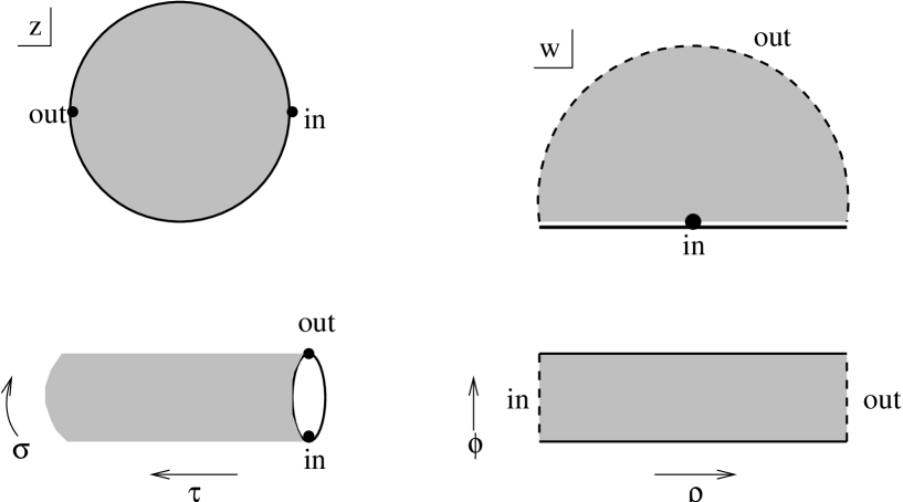
Figure 1: The conformal transformation that maps the half-infinite cylinder to the strip can be decomposed into three successive steps: $\sigma+i\tau_{E}=-\frac{i}{2}\;{\rm log}z$, then $iw=(z-1)/(z+1)$ , and finally $\rho_{E}+i\phi={\rm log}w$. Open-string vertex operators are inserted at points ‘in’ and ‘out’.

Eq. (40) should be compared to the expression (16) for the boundary state. The main difference is that the argument of $A^{i}$ in the Wilson-loop operator has been shifted by the imaginary amount ${ip^{+}}\log|\tan\sigma|$. Since $A^{i}$ is a priori defined for real $x^{+}$, we need to evaluate the $\sigma$-integral by an appropriate analytic continuation. Our main point is that this analytic continuation is determined by the causal structure of the Lorentzian open-string world-sheet. Indeed, what enters in the argument of $A^{i}$ is the boundary restriction of the conformal transformation

$$\rho_{E}+i\phi={\rm log}({\rm tan}(\sigma+i\tau_{E}))$$ (41)

that maps the Euclidean half-infinite cylinder, $\sigma\in[0,\pi)$ and $\tau_{E}\in[0,\infty]$, to the Euclidean infinite strip, $\phi\in[0,\pi]$ and $\rho_{E}\in[-\infty,\infty]$; this mapping is illustrated in figure 1. As $\sigma$ runs from $\mathrm{𝟎}$ to $\pi$, $\rho_{E}(\sigma)$ covers the real axis twice, corresponding to the two boundaries ($\phi=0$ and $\pi$) of the strip. The form of the argument in (40) suggests that the necessary analytic continuation should amount to a Wick rotation of the (preferred) open-string time of the strip world-sheet.

To see how this works in detail, we first apply the reasoning of section 3 to eliminate the positive-frequency modes of $X^{i}$ and to arrive at an expression like (3). Since the negative-frequency modes annihilate the bra vacuum we find :

$$S_{0\to 0}=\frac{\cal N}{4}\,\langle 0|\exp\Bigl{(}-\int_{0}^{\pi}d\sigma\; \hskip-8.5359ptA^{i}\Bigl{(}x^{+}_{c}+ip^{+}\rho_{E}(\sigma)\Bigr{)}\;\int_{0}^{\pi}d\sigma^{\prime}\;A^{i}\Bigl{(}x^{+}_{c}+ip^{+}\rho_{E}(\sigma^{\prime})\Bigr{)}\;\times$$ (42)

$$\times\;\partial_{\sigma}\partial_{\sigma^{\prime}}D_{E}^{\rm cyl}(\sigma,\sigma^{\prime})\Bigr{)}\;|\!|{\rm Dp}\rangle\!\rangle\;.$$

We have here replaced the Feynman propagator on the cylinder by its Euclidean counterpart, since the two coincide for space-like separations. Furthermore, since the closed-string time does not enter in (42) we may assume that the world-sheet is Euclidean. Next we perform the conformal transformation (41) which maps the integration contours to the oriented boundary of the Euclidean strip. The transformation of the $\sigma$ and $\sigma^{\prime}$ derivatives in the above expression cancels precisely the two Jacobians from the integration measures. The equal-time propagator on the cylinder is furthermore mapped to the boundary propagator of the Euclidean strip as follows :

$$D_{E}^{\rm cyl}(\sigma,\sigma^{\prime})\ \rightarrow\ {1\over 2}D_{E}^{\rm str}(\rho_{E}-\rho_{E}^{\prime},\phi_{0})+f(\rho_{E})+f(\rho_{E}^{\prime})\ ,$$ (43)

where $f(x)={1\over 4}\log\cosh x$, and $\phi_{0}=0$ or $\pi$ for points on the same or opposite boundaries of the strip. The relation (43) is discussed in detail in the appendix. Plugging this in the expression (42) gives :

$$S_{0\to 0}=\frac{\cal N}{4}\,\langle 0| \exp\Bigl{(}-\int_{-\infty}^{\infty}d\rho_{E}\;A^{i}\Bigl{(}x^{+}_{c}+ip^{+}\rho_{E}\Bigr{)}\;\int_{-\infty}^{\infty}d\rho_{E}^{\prime}\;A^{i}\Bigl{(}x^{+}_{c}+ip^{+}\rho_{E}^{\prime}\Bigr{)}\;\times$$ (44)

$$\times\;\partial_{\rho_{E}}\partial_{\rho_{E}^{\prime}}\left[D_{E}^{\rm str}(\rho_{E}-\rho_{E}^{\prime},0)-D_{E}^{\rm str}(\rho_{E}-\rho_{E}^{\prime},\pi)\right]\Bigr{)}\;|\!|{\rm Dp}\rangle\!\rangle\;.$$

Note that the extra terms in the right-hand side of (43) dropped out upon derivation, while the relative factor of $1/2$ took precisely care of the fact that as $\sigma$ runs over $[0,\pi)$, the strip time covers the real axis twice.

The expression (44) should be compared with the result of section 2 : $S_{0\to 0}=e^{i\delta_{1}-\delta_{2}}$ with $\delta_{1}+i\delta_{2}$ given by eq. (7). The two results indeed agree if we Wick rotate

$$\rho_{E}\to-i\rho\ \ ,$$ (45)

thereby sending the Euclidean to the Feynman propagator. The $x^{+}_{c}$ in the arguments of the $A^{i}$ can be, of course, absorbed in the integration variables, and we must also use our condition on ${\cal N}$. This completes the proof of open/closed-string duality for this particular process. Other one-to-one S-matrix elements can be analysed in a similar way.

A subtle point in the above derivation concerns possible singularities of the profile functions $A^{i}$ in the complex plane, which could a priori obstruct the Wick rotation of the integration contour. Strictly speaking the right-hand-side of the BCH formula (38) is defined by a Taylor expansion in powers of the commutator $[C,B]$. As a result, the background fields in eq. (42) are also defined as Taylor series around the point on the real axis $x^{+}_{c}$. The Wick rotation $\rho_{E}\to-i\rho$ makes each term in these expansions real. Singularities of $A^{i}$ in the complex plane may limit the radius of convergence of these series. However these series still determine unique continuous functions on the integration axis which obviously coincide with the original wave profiles.

In summary we note that (as expected) the Euclidean world-sheet calculation gives the same result whether performed in the open- or in the closed-string channel. The passage to a Lorentzian world-sheet must, on the other hand, be done by Wick rotating the time coordinate of the open channel. This is the choice that leads to a globally consistent causal structure on the string worldsheet. [The closed-channel time comes to an ’abrupt’ end on the disc boundary]. We turn now to the more general situation, in which there are several incoming and/or outgoing strings.

5 Multi-string tree amplitudes

The boundary-state calculation of the previous section can be generalized easily to tree-level amplitudes involving arbitrary numbers of open strings. Let $i=1,\ldots,N$ label the incoming open strings while the outgoing open strings are labelled by $i=N+1,\ldots,N+M$. Each string carries a fraction $\alpha_{i}$ of the conserved $p^{+}$ momentum ; thus by construction we have $\sum_{i=1}^{N}\alpha_{i}=\sum_{j=N+1}^{N+M}\alpha_{j}=1$. For simplicity we will take all these open strings to be in their tachyonic ground state, and to have vanishing transverse momentum.

The amplitude (31) is now replaced by a more general expression, where incoming and outgoing open strings are represented by vertex operators inserted at angular positions $\sigma_{i}$ on the circle. Three of the $N+M$ insertion points, for instance $\sigma_{1},\sigma_{2}$ and $\sigma_{3}$, can be fixed using the SL$(2,\mathbb{R})$ invariance of the disc. The total amplitude is obtained by integrating over the remaining $N+M-3$ positions. Since we consider here a single Dp-brane, we do not worry about Chan-Paton matrices.

Following the same reasoning as in section 4, one finds that this disc diagram equals

$$S_{{0\cdots 0}\rightarrow 0\cdots 0}=\left(\prod_{i=4}^{N+M}\int_{0}^{\pi}d\sigma_{i}\right)\;\prod_{i>j} e^{-p_{i}\cdot p_{j}D_{E}^{\rm cyl}(\sigma_{i},\sigma_{j})}\,\times$$ (46)

$$\times\langle 0|\exp\Bigl{(}-\int_{0}^{\pi}d\sigma\;A^{i}\Bigl{(}x^{+}_{c}+ip^{+}\rho_{E}\Bigr{)}\; \hskip-8.5359pt\int_{0}^{\pi}d\sigma^{\prime}\;A^{i}\Bigl{(}x^{+}_{c}+ip^{+}\rho_{E}^{\prime}\Bigr{)}\;\partial_{\sigma}\partial_{\sigma^{\prime}}D_{E}^{\rm cyl}(\sigma,\sigma^{\prime})\Bigr{)}\;|\!|{\rm Dp}\rangle\!\rangle\;,$$

where $\rho_{E}(\sigma)$ is now given by the following expression:

$$\rho_{E}(\sigma)=\sum_{i=1}^{N}2\alpha_{i}\,D_{E}^{\rm cyl}(\sigma,\sigma_{i})-\sum_{i=N+1}^{N+M}2\alpha_{i}\,D_{E}^{\rm cyl}(\sigma,\sigma_{i})\,,$$ (47)

while $\rho_{E}^{\prime}$ is the same function with $\sigma$ replaced by $\sigma^{\prime}$. The function defined by (47) is the restriction to the boundary of the map between the half-infinite cylinder with $N+M$ marked points on the boundary, and the open-string diagram in light-cone gauge. The latter is an infinite strip with cuts which extend either to $\rho_{E}=-\infty$ or to $\rho_{E}=+\infty$. This transformation is illustrated for $N=1$ and $M=2$ in figure 2.

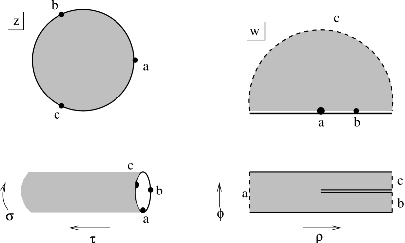
Figure 2: The transformation (47) from the half-infinite cylinder to the strip in the case of one incoming and two outgoing strings. The first two steps are the same as in figure 1, while the map from the $w$ plane to the cut-strip is a ‘Schwarz-Christoffel transformation’ (see for example [49]).

The rest of the calculation should then proceed as in the previous section: one first changes integration variables from $\sigma$ to the open world-sheet time $\rho_{E}$. All integration contours run now around the oriented boundary of the cut-strip. Mass-shell conditions and momentum conservation should ensure that Jacobians and extra terms in the transformed propagators cancel. Finally, the form of the argument of the $A^{i}$ shows that the Wick rotation should be done in the time coordinate, $\rho_{E}$, of the cut strip. We believe (but have not checked explicitly) that for more general diagrams, with loops and/or with asymptotic closed-string states, it is always the light-cone gauge worldsheet that singles out the ’prefered’, Wick-rotated time.

We postpone the explicit calculation of these amplitudes, including the case where the emitted open strings are gauge bosons or gravitons, to future work [50]. A subtle point, to which we hope to return, concerns the causal propagator on a cut world-sheet. The study of potential divergences of these amplitudes, and more generally of the physics of back reaction, is especially interesting for the reasons exposed in ref. [17].

Appendix A Relation between world-sheet propagators

In this appendix we establish explicitly the relation between the two-point functions on the cylinder and on the strip, which enters in the derivation of the single-open-string S-matrix from the boundary state.

The Feynman propagator on the strip for a scalar field with Neumann boundary conditions has the following standard representation :

$$D_{F}^{\rm str}(\lambda,\phi)=\sum_{n=-\infty}^{\infty}\int\frac{d\omega}{2\pi}\;\frac{i}{\omega^{2}-n^{2}+i\epsilon}\;e^{-i\omega\lambda+in\phi}\ .$$ (48)

By performing the $\omega$ integration one recovers the expression (9) in the main text (for $\phi=0,\pi$). Wick rotating the world-sheet time (i.e.  replacing $\omega\mapsto i\omega$ and $\lambda\mapsto i\lambda_{E}$) leads to the Euclidean propagator

$$D_{E}^{\rm str}(\lambda_{E},\phi)=\sum_{n=-\infty}^{\infty}\int\frac{d\omega}{2\pi}\;\frac{1}{\omega^{2}+n^{2}}\;e^{i\omega\lambda_{E}+in\phi}\ .$$ (49)

On the boundaries of the strip this reads (up to a constant)

$$D_{E}^{\rm str}(\lambda_{E},\phi_{0})=-\log\left|e^{\lambda_{E}/2}\mp e^{-\lambda_{E}/2}\right|\ ,$$ (50)

where the minus and plus signs correspond, respectively, to $\phi_{0}=0$ and $\phi_{0}=\pi$.

The Euclidean propagator (50) should be compared with the equal-time two-point function on the cylinder

$$D_{E}^{\rm cyl}(\sigma,\sigma^{\prime})=-\frac{1}{4}\;{\rm log}\;\left(4\;{\rm sin}^{2}(\sigma-\sigma^{\prime})\right)\ ,$$ (51)

where $\lambda_{E}$ is to be identified with $\lambda_{E}=\rho_{E}(\sigma)-\rho_{E}(\sigma^{\prime})$. Note that for equal times the Feynman and Euclidean propagators coincide. Inverting the relation $\rho_{E}+i\phi_{0}={\rm log(tan}\sigma)$, which maps the boundaries of the half-infinite cylinder and the infinite strip, gives

$$e^{-2i\sigma}=\frac{1\mp ie^{\rho_{E}}}{1\pm ie^{\rho_{E}}}\ ,$$ (52)

where the choice of sign refers to the two possible values of $\phi_{0}$. Plugging this into (51) and doing some straightforward algebra one finds

$$D_{E}^{\rm cyl}=-\frac{1}{2}\log\left|e^{\lambda_{E}/2}\mp e^{-\lambda_{E}/2}\right|+\frac{1}{4}{\log\cosh\rho_{E}}+\frac{1}{4}{\log\cosh\rho_{E}^{\prime}}\ .$$ (53)

This differs from (50) in two ways: (i) there is a relative factor of 2 between the open- and closed-string two-point functions coming from the contribution of mirror images when the insertion points approach the boundary; and (ii) there are extra terms, due to the fact that $X$ is not a conformal primary field, and which will drop out when one considers the primary field $\partial X$.

As is explained in the main text, the factor of $2$ is precisely what is needed to relate (42) to (44). Indeed, since $\rho_{E}(\sigma)=\rho_{E}(\pi-\sigma)$, the integrals in (42) cover the integration domain in (44) twice. Furthermore, since only the derivatives of the propagators appear, the extra terms in (53) do not contribute. This proves, after a Wick rotation, the desired equality between the open- and the closed-channel calculations of the S-matrix.

References

- [1] A. Strominger, “SD-branes in string theory,” talk given at ‘Strings 2003’, Kyoto, Japan [http://www2.yukawa.kyoto-u.ac.jp/str2003/talks/strominger.pdf].
- [2] A. Sen, “Closed strings and unstable D-branes,” talk given at ‘Strings 2003’, Kyoto, Japan [http://www2.yukawa.kyoto-u.ac.jp/str2003/talks/sen.pdf].
- [3] J. Maldacena, “Closed strings from decaying D-branes,” talk given at ‘Strings 2003’, Kyoto, Japan [http://www2.yukawa.kyoto-u.ac.jp/str2003/talks/maldacena.pdf].
- [4] G.T. Horowitz and A.R. Steif, “Singular string solutions with nonsingular initial data,” Phys. Lett. B 258 (1991) 91.
- [5] J. Khoury, B.A. Ovrut, N. Seiberg, P.J. Steinhardt and N. Turok, “From big crunch to big bang,” Phys. Rev. D 65 (2002) 086007 [arXiv:hep-th/0108187].
- [6] J. Figueroa-O’Farrill and J. Simon, “Generalized supersymmetric fluxbranes,” JHEP 0112 (2001) 011 [arXiv:hep-th/0110170].
- [7] L. Cornalba and M.S. Costa, “A new cosmological scenario in string theory,” Phys. Rev. D 66 (2002) 066001 [arXiv:hep-th/0203031].
- [8] N. Nekrasov, “Milne universe, tachyons, and quantum group,” arXiv:hep-th/0203112.
- [9] H. Liu, G. Moore and N. Seiberg, “Strings in a time-dependent orbifold,” JHEP 0206 (2002) 045 [arXiv:hep-th/0204168]; “Strings in time-dependent orbifolds,” JHEP 0210 (2002) 031 [arXiv:hep-th/0206182].
-
[10]
B. Craps, D. Kutasov and G. Rajesh,
“String propagation in the presence
of cosmological singularities,”
JHEP 0206 (2002) 053
[arXiv:hep-th/0205101];
M. Berkooz, B. Craps, D. Kutasov and G. Rajesh, “Comments on cosmological singularities in string theory,” JHEP 0303 (2003) 031 [arXiv:hep-th/0212215]. - [11] A. Lawrence, “On the instability of 3D null singularities,” JHEP 0211 (2002) 019 [arXiv:hep-th/0205288].
- [12] G.T. Horowitz and J. Polchinski, “Instability of spacelike and null orbifold singularities,” Phys. Rev. D 66 (2002) 103512 [arXiv:hep-th/0206228].
-
[13]
M. Fabinger and J. McGreevy,
“On smooth time-dependent orbifolds and null singularities,”
JHEP 0306 (2003) 042 [arXiv:hep-th/0206196];
M. Fabinger and S. Hellerman, “Stringy resolutions of null singularities,” arXiv:hep-th/0212223. - [14] E. Dudas, J. Mourad and C. Timirgaziu, “Time and space dependent backgrounds from nonsupersymmetric strings,” Nucl. Phys. B 660 (2003) 3 [arXiv:hep-th/0209176].
- [15] S. Elitzur, A. Giveon and E. Rabinovici, “Removing singularities,” JHEP 0301 (2003) 017 [arXiv:hep-th/0212242].
- [16] M. Berkooz and B. Pioline, “Strings in an electric field, and the Milne universe,” arXiv:hep-th/0307280.
- [17] C. Bachas and C. Hull, “Null brane intersections,” JHEP 0212 (2002) 035 [arXiv:hep-th/0210269].
- [18] R.C. Myers and D.J. Winters, “From D-Dbar pairs to branes in motion,” JHEP 0212 (2002) 061 [arXiv:hep-th/0211042].
- [19] B. Chen, C.-M. Chen and F.-L. Lin, “Supergravity null scissors and super-crosses,” JHEP 0304 (2003) 022 [arXiv:hep-th/0303156].
- [20] C.G. Callan, J.M. Maldacena and A.W. Peet, “Extremal black holes as fundamental strings,” Nucl. Phys. B 475 (1996) 645 [arXiv:hep-th/9510134].
- [21] A. Dabholkar, J.P. Gauntlett, J.A. Harvey and D. Waldram, “Strings as solitons and black holes as strings,” Nucl. Phys. B 474 (1996) 85 [arXiv:hep-th/9511053].
- [22] C.G. Callan and I.R. Klebanov, “D-brane boundary state dynamics,” Nucl. Phys. B 465 (1996) 473 [arXiv:hep-th/9511173].
-
[23]
D. Mateos and P.K. Townsend,
“Supertubes,”
Phys. Rev. Lett. 87 (2001) 011602
[arXiv:hep-th/0103030];
D. Mateos, S. Ng and P.K. Townsend, “Supercurves,” Phys. Lett. B 538 (2002) 366 [arXiv:hep-th/0204062]. -
[24]
O. Lunin and S.D. Mathur,
“Metric of the multiply wound rotating string,”
Nucl. Phys. B 610 (2001) 49
[arXiv:hep-th/0105136];
O. Lunin, J. Maldacena and L. Maoz, “Gravity solutions for the D1-D5 system with angular momentum,” arXiv:hep-th/0212210. - [25] J.H. Cho and P. Oh, “Super D-helix,” Phys. Rev. D 64 (2001) 106010 [arXiv:hep-th/0105095].
-
[26]
Y. Hyakutake and N. Ohta,
“Supertubes and supercurves from M-ribbons,”
Phys. Lett. B 539 (2002) 153
[arXiv:hep-th/0204161];
D. s. Bak and N. Ohta, “Supersymmetric D2 anti-D2 strings,” Phys. Lett. B 527 (2002) 131 [arXiv:hep-th/0112034];
D. s. Bak, N. Ohta and M. M. Sheikh-Jabbari, “Supersymmetric brane anti-brane systems: Matrix model description, stability and decoupling limits,” JHEP 0209 (2002) 048 [arXiv:hep-th/0205265]. - [27] C. Bachas, “Relativistic string in a pulse,” Annals Phys. 305 (2003) 286 [arXiv:hep-th/0212217].
- [28] B. Durin and B. Pioline, “Open strings in relativistic ion traps,” JHEP 0305 (2003) 035 [arXiv:hep-th/0302159].
- [29] A. Dabholkar and S. Parvizi, “Dp branes in pp-wave background,” Nucl. Phys. B 641 (2002) 223 [arXiv:hep-th/0203231].
- [30] D. Berenstein, E. Gava, J.M. Maldacena, K.S. Narain and H. Nastase, “Open strings on plane waves and their Yang-Mills duals,” arXiv:hep-th/0203249.
- [31] A. Kumar, R.R. Nayak and Sanjay, “D-brane solutions in pp-wave background,” Phys. Lett. B 541 (2002) 183 [arXiv:hep-th/0204025].
- [32] K. Skenderis and M. Taylor, “Branes in AdS and pp-wave spacetimes,” JHEP 0206 (2002) 025 [arXiv:hep-th/0204054] ; “Open strings in the plane wave background. I: Quantization and symmetries,” arXiv:hep-th/0211011.
-
[33]
O. Bergman, M.R. Gaberdiel and M.B. Green,
“D-brane interactions in type IIB plane-wave background,”
JHEP 0303 (2003) 002
[arXiv:hep-th/0205183];
M.R. Gaberdiel and M.B. Green, “The D-instanton and other supersymmetric D-branes in IIB plane-wave string theory,” arXiv:hep-th/0211122. - [34] P. Bain, K. Peeters and M. Zamaklar, “D-branes in a plane wave from covariant open strings,” Phys. Rev. D 67 (2003) 066001 [arXiv:hep-th/0208038].
- [35] G. Sarkissian and M. Zamaklar, “Diagonal D-branes in product spaces and their Penrose limits,” arXiv:hep-th/0308174.
- [36] D. Amati and C. Klimcik, “Strings in a shock wave background and generation of curved geometry from flat space string theory,” Phys. Lett. B 210 (1988) 92.
- [37] R.R. Metsaev, “Type IIB Green-Schwarz superstring in plane wave Ramond-Ramond background,” Nucl. Phys. B 625 (2002) 70 [arXiv:hep-th/0112044].
- [38] G. Papadopoulos, J.G. Russo and A.A. Tseytlin, “Solvable model of strings in a time-dependent plane-wave background,” Class. Quant. Grav. 20 (2003) 969 [arXiv:hep-th/0211289].
- [39] C. Itzykson and J.B. Zuber, “Quantum Field Theory,” (McGraw-Hill 1980).
- [40] Y. Hikida, H. Takayanagi and T. Takayanagi, “Boundary states for D-branes with traveling waves,” JHEP 0304 (2003) 032 [arXiv:hep-th/0303214].
- [41] J.D. Blum, “Gravitational radiation from travelling waves on D-strings,” arXiv:hep-th/0304173.
- [42] H. Takayanagi, “Boundary states for supertubes in flat spacetime and Goedel universe,” arXiv:hep-th/0309135.
- [43] O. D. Andreev and A. A. Tseytlin, “Partition Function Representation For The Open Superstring Effective Action: Cancellation Of Mobius Infinities And Derivative Corrections To Born-Infeld Lagrangian,” Nucl. Phys. B 311 (1988) 205.
- [44] E. Witten, “Some computations in background independent off-shell string theory,” Phys. Rev. D 47 (1993) 3405 [arXiv:hep-th/9210065].
- [45] S.L. Shatashvili, “Comment on the background independent open string theory,” Phys. Lett. B 311 (1993) 83 [arXiv:hep-th/9303143].
- [46] J. Schulze, “Coulomb gas on the half plane,” Nucl. Phys. B 489 (1997) 580 [arXiv:hep-th/9602177].
- [47] G.M.T. Watts, “On the boundary Ising model with disorder operators,” Nucl. Phys. B 596 (2001) 513 [arXiv:hep-th/0002218].
- [48] S. Kawai, “Free-field realisation of boundary states and boundary correlation functions of minimal models,” J. Phys. A 36 (2003) 6547 [arXiv:hep-th/0210032].
- [49] M.B. Green, J.H. Schwarz and E. Witten, “Superstring Theory, Volume 2,” (Cambridge University Press 1987).
- [50] C. Bachas, N. Couchoud and M. Gaberdiel, work in progress.