The Whitham Deformation of the Dijkgraaf-Vafa Theory

Abstract:

We discuss the Whitham deformation of the effective superpotential in the Dijkgraaf-Vafa (DV) theory. It amounts to discussing the Whitham deformation of an underlying (hyper)elliptic curve. Taking the elliptic case for simplicity we derive the Whitham equation for the period, which governs flowings of branch points on the Riemann surface. By studying the hodograph solution to the Whitham equation it is shown that the effective superpotential in the DV theory is realized by many different meromorphic differentials. Depending on which meromorphic differential to take, the effective superpotential undergoes different deformations. This aspect of the DV theory is discussed in detail by taking the $N=1^{*}$ theory. We give a physical interpretation of the deformation parameters.

1 Introduction

One of the long-standing problems in the quantum field theory is to understand non-perturbative dynamics of the supersymmetric QCD. The recent works by Dijkgraaf and Vafa[1, 2] have given a breakthrough towards to this direction. They found a close relation between the $N=1$ supersymmetric QCD and a matrix model. It is now confirmed by subsequent works by many people. This Dijkgraaf-Vafa theory revived a renewed attention[3, 4] to the Seiberg-Witten theory (SW) for the $N=2$ supersymmetric QCD[5]. Indeed both theories have relevance to the Riemann surface and the Whitham hierarchy as commonly underlying features. To be concrete, take the case which is concerned about the Riemann surface with genus one. The DV theory gives an effective superpotential of the $N=1$ supersymmetric QCD

$$W_{DV}=\int d^{2}\theta\ (N{\partial{\cal F}_{0}\over\partial S}-2\pi i{\mathop{\tau}^{\circ}}S),$$ (1)

which is the perturbative part of the Veneziano-Yankielovicz superpotential. On the other hand the SW theory gives the effective action of the $N=2$ supersymmetric QCD

$$W_{SW}={1\over 4\pi}{\rm Im}[\int d^{4}\theta\ {\partial{\cal F}_{0}(A)\over\partial A}\bar{A}+\int d^{2}\theta\ {1\over 2}\tau_{0}(A)W_{\alpha}W^{\alpha}].$$ (2)

In (1) and (2) ${\cal F}_{0}$ is called the free energy and characterized by a certain differential on an elliptic curve. In (2) $\tau_{0}(A)$ is the period of the curve.

Since the SW theory was born, the Whitham hierarchy attracted attention as a underlying integrable structure in the SW theory[6, 7, 8]. But dynamical aspects of the hierarchy was not properly studied. Dynamical flowings of branch points of the Riemann surface and the consequent creation or annihilation of branch cuts were the original concerns to study the Whitham hierarchy[9]. There people aimed regulation (or modulation) of singular behaviors of finite-gap solutions for the KdV system. We think it important to shed more light on this aspect of the DV and SW theories in the revived era of the interest. In this paper we study the Whitham deformation of the elliptic curve as a flow of the branch points on the Riemann surface. We will show that the flow is governed by the Whitham equation for the period $\tau$ of the curve (5), i.e.,

$${\partial\tau(a,\vec{T})\over\partial T_{M}}=s_{M}(\tau(a,\vec{T})){\partial\tau(a,\vec{T})\over\partial a},\quad\quad\tau(a,\vec{0})\equiv\tau_{0}(a).$$ (3)

Here $\vec{T}=(T_{1},T_{2},\cdots)$ and $a$ is either $S$ for the DV theory or $A$ for the SW theory. $s_{1}(\tau(a,\vec{T})),s_{2}(\tau(a,\vec{T})),\cdots$, are the characteristic speeds. (For more explanations see the discussion thereabout.) It is noteworthy that the Whitham equation looks like the renormalization group equation for the running coupling

$${\partial\bar{g}(t,g)\over\partial t}=\beta(g){\partial\bar{g}(t,g)\over\partial g}.$$

In the recent papers[10] they developed interesting arguments on an underlying integrable structure of the DV theory. Namely they discussed that the equilibria of the superpotential of the DV theory, (1), correspond to the stable flow points of some integrable systems at which the relevant (hyper)elliptic curve degenerates. But the flow is not the one given by the Whitham deformation (3), which is of interest in this paper.

It is known[11] that the equation of the type (3) admits a hodograph solution as a special solution and it is characterized by a free energy ${\cal F}$. We will find that the initial condition $\tau_{0}(a)$ of a hodograph solution is imposed by specifying the inverse function $a(\tau_{0})(\equiv\tau_{0}^{-1}(a))$ as (6), i.e.,

$$a(\tau(a,\vec{0}))=\sum_{M=1}^{M_{0}}\Lambda_{M}s_{M}(\tau(a,\vec{0})).$$ (4)

It will be shown that (4) is given as a period integral of a certain differential, which is nothing but the DV or SW differential. Then the free energy ${\cal F}_{0}$ in (1) and (2) is an initial value of the free energy ${\cal F}$ which characterizes the hodograph solution

$${\cal F}_{0}(a)={\cal F}|_{\vec{T}=0}.$$ (5)

Choosing a set of non-vanishing $\Lambda_{M}$ in (4) uniquely specifies the initial condition $\tau_{0}(a)$ and therefore the free energy ${\cal F}_{0}(a)$. Here the characteristic speeds $s_{M}(\tau(a,\vec{0})),M=1,2,\cdots$, were kept fixed. Now we reverse the argument. Namely we fix the initial condition $\tau_{0}(a)$, that is, the l.h.s. of (4), and specify the characteristic speeds so as to satisfy (4) for the chosen set of $(\Lambda_{1},\Lambda_{2},\cdots,\Lambda_{M_{0}})$. We show that it can be done by changing parameterization of the elliptic curve. Then the fixed initial condition $\tau_{0}(a)$ is given by different DV or SW differentials. The hodograph solution $\tau(a,\vec{T})$ is characterized by different free energies ${\cal F}$. But the key point is that its initial value ${\cal F}_{0}(a)$ remains fixed as $\tau_{0}(a)={\partial^{2}{\cal F}_{0}\over\partial a^{2}}$. In other words a fixed ${\cal F}_{0}(a)$ undergoes different Whitham deformations depending on the choice of $(\Lambda_{1},\Lambda_{2},\cdots,\Lambda_{M_{0}})$. To discuss concretely this aspect of the DV theory, we will take the $N=1^{*}$ theory[2, 12] as an example. We will explicitly give the superpotential of the theory by various DV differentials, and show the possibility of different Whitham deformations.

The paper is organized as follows. In Section 2 we define quantities $\tau_{MN}$ as extensions of the period $\tau(\equiv\tau_{00})$ of the elliptic curve. They are important constituents in the paper. In Section 3 we discuss on a “gauge” freedom in parameterizing the elliptic curve. Fixing this freedom we find an equation for the curve, which plays a fundamental role in the paper. In Section 4 we think of deforming the curve. We introduce the Whitham hierarchy to the deformation. It is shown to amount to assuming the Whitham equation (3). The Whitham hierarchy is mimic to the dispersionless KP hierarchy in the topological field theory[13, 14, 15]. Therefore it may be formulated by means of analogous quantities with the 2-point functions of the topological field theory. We find them by modifying $\tau_{MN}$, discussed in Section 2. In Section 5 we study the hodograph solution to the Whitham equation according to [11, 15]. We then interpret the solution in terms of the topological field theory, i.e., by employing the terminology like the free energy, the small or large phase space etc. In Section 6 the dual version of the Whitham equation is discussed. The initial condition for the hodograph solution is characterized by the DV or SW differential. In the basis of these arguments we discuss various Whitham deformations of the $N=1^{*}$ theory in Section 7. In Section 8 we give a matrix-model interpretation of those Whitham deformations. Appendix A is devoted to give a short summary on the elliptic curve and some useful formulae for the period integral. In Appendix B we discuss a systematic method to evaluate the 2-point functions $\tau_{MN}$. In Appendix C we give some calculations to check the consistency of the formalism for the Whitham hierarchy, developed in this paper.

2 The elliptic curve

Throughout the paper we consider an elliptic curve defined by

$$y^{2}=4(x-u)(x-v)(x-w).$$ (1)

It may be also given by

$$y^{2}=4(x-\lambda_{1})(x-\lambda_{2})(x-\lambda_{3})(x-\lambda_{4}).$$

But this reduces to (1) by the change

$${1\over x-\lambda_{4}}\longrightarrow x,\quad\quad\quad{y\over\sqrt{(\lambda_{4}-\lambda_{1})(\lambda_{4}-\lambda_{2})(\lambda_{4}-\lambda_{3})}}\longrightarrow{y\over x^{2}}.$$

On the curve (1) there exists one holomorphic differential $d\omega_{0}$ of the form

$$d\omega_{0}={1\over g_{0}}{dx\over y}.$$ (2)

By the normalization

$$\oint_{A}d\omega_{0}=1,$$ (3)

$g_{0}$ is fixed to be

$$g_{0}=\oint_{A}{dx\over y}.$$ (4)

The period on the curve is given by

$$\tau = \oint_{B}d\omega_{0}={g_{D0}\over g_{0}},$$ (5)

with

$$g_{D0}=\oint_{B}{dx\over y}.$$

On the curve there exists also a set of meromorphic differentials $d\Omega_{M},M=1,2,\cdots,$ of the form

$$d\Omega_{M} = [x^{M}+\gamma_{M-1}x^{M-1}+\cdots+\gamma_{1}x+\gamma_{0}]{dx\over y}$$

$$\equiv Q_{M}(x){dx\over y}.$$

The coefficients $\gamma_{M-1},\cdots,\gamma_{0}$ of the polynomial $Q_{M}$ is uniquely determined by requiring $d\Omega_{M}$ to satisfy

$$\oint_{A}d\Omega_{M}=0,$$ (7)

and to have poles at $x={1\over\xi^{2}}=\infty$ such that

$$d\Omega_{M}=-\xi^{-2M}d\xi+holomorphic.$$ (8)

It is done by the recursive formula (3) and (11).

Let us introduce the following quantities as an extension of the period (5):

$$\tau_{0M} \equiv \tau_{M0}$$ (9)

$$= \oint_{B}d\Omega_{M},\quad\quad\quad M=1,2,\cdots.$$

It becomes

$$\tau_{0M}=-2\pi i\ {\rm res}_{\xi=0}[{\scriptstyle{\xi^{-2M+1}}\over\scriptstyle{2M-1}}d\omega_{0}],$$ (10)

by the Riemann bilinear relation. By the analogy we also introduce the quantities

$$\tau_{NM}=-2\pi i\ {\rm res}_{\xi=0}[{\scriptstyle{\xi^{-2M+1}}\over\scriptstyle{2M-1}}d\Omega_{N}],\quad\quad M,N=1,2,\cdots.$$ (11)

Using the Riemann bilinear relation again we have

$$\tau_{NM}=\tau_{MN}.$$ (12)

These quantities will be important constituents in our discussions later.

3 Gauge fixing and the fundamental equation

Let us assume that the branch points of (1) are parameterized by one parameter alone, namely the period as $u(\tau),v(\tau),w(\tau)$. In general an elliptic curve is determined by $g_{0}$ and $g_{D0}$. The assumption implies that they are functions of $\tau$. To realize the assumption it suffices to set $g_{0}$ to be a particular function of $\tau$, because they are related by (5). We call it “gauge fixing”, which is an abusive terminology. For instance, with the “gauge” $g_{0}=2\pi$ the branch points of the curve are expressed as

$$u(\tau) = {c\over 3}+{1\over 12}[\theta_{3}(\tau)^{4}+\theta_{0}(\tau)^{4}],$$

$$v(\tau) = {c\over 3}+{1\over 12}[\theta_{2}(\tau)^{4}-\theta_{0}(\tau)^{4}],$$ (1)

$$w(\tau) = {c\over 3}-{1\over 12}[\theta_{2}(\tau)^{4}+\theta_{3}(\tau)^{4}],$$

by using the Weierstrass standard form (1) and (2). Here $c$ is given by

$$c=u(\tau)+v(\tau)+w(\tau),$$ (2)

which is still to be fixed arbitrarily. We can also take the “gauge” which sets one of the branch points, for instance, $w(\tau)=1$. Then we have

$$u(\tau) = {c\over 3}+{1\over 3}({\pi\over g_{0}})^{2}[\theta_{3}(\tau)^{4}+\theta_{0}(\tau)^{4}],$$

$$v(\tau) = {c\over 3}+{1\over 3}({\pi\over g_{0}})^{2}[\theta_{2}(\tau)^{4}-\theta_{0}(\tau)^{4}],$$ (3)

where $g_{0}$ is given by

$$1={c\over 3}-{1\over 12}({\pi\over g_{0}})^{2}[\theta_{2}(\tau)^{4}+\theta_{3}(\tau)^{4}].$$

With the former “gauge” the three branch points $u(\tau),v(\tau),w(\tau)$ move depending $\tau$. Instead with the latter one only two of them move.

When the branch points $u(\tau),v(\tau),w(\tau)$ are given as such, we can show the fundamental equation throughout the paper:

$${\partial\over\partial\tau}d\Omega_{M}(x)=s_{M}(\tau){\partial\over\partial\tau}d\omega_{0}+d[\Delta_{M}(x,\tau)].\quad\quad M=1,2,\cdots.$$ (4)

Here $s_{M}(\tau)$ in the first term is the characteristic speed given by

$$s_{M}(\tau)=g_{0}{Q_{M}(u)u^{\prime}(v-w)+Q_{M}(v)v^{\prime}(w-u)+Q(w)_{M}w^{\prime}(u-v)\over u^{\prime}(v-w)+v^{\prime}(w-u)+w^{\prime}(u-v)},$$ (5)

and the second term is an exact form with

$$\Delta_{M}(x,\tau)= - {Q_{M}(u)u^{\prime}(v^{\prime}w-w^{\prime}v)+Q_{M}(v)v^{\prime}(w^{\prime}u-u^{\prime}w)+Q_{M}(w)w^{\prime}(u^{\prime}v-v^{\prime}u)\over u^{\prime}(v-w)+v^{\prime}(w-u)+w^{\prime}(u-v)}{1\over y}$$ (6)

$$+ {Q_{M}(u)u^{\prime}(v^{\prime}-w^{\prime})+Q_{M}(v)v^{\prime}(w^{\prime}-u^{\prime})+Q_{M}(w)w^{\prime}(u^{\prime}-v^{\prime})\over u^{\prime}(v-w)+v^{\prime}(w-u)+w^{\prime}(u-v)}{x\over y}.$$

To prove (4), first of all note that (8) implies that ${\partial\over\partial\tau}d\Omega_{M}(x)$ is holomorphic. Therefore we have

$${\partial\over\partial\tau}d\Omega_{M}(x)$$ (7)

$$\hskip 28.45274pt={\partial Q_{M}(x)\over\partial\tau}{dx\over y}+Q_{M}(x){\partial\over\partial\tau}{dx\over y}$$

$$\hskip 28.45274pt=[A_{M}(u,v,w)+{1\over 2}({u^{\prime}Q_{M}(u)\over x-u}+{v^{\prime}Q_{M}(v)\over x-v}+{w^{\prime}Q_{M}(w)\over x-w})]{dx\over y},$$

with some functions $A_{M}(u,v,w)$. On the other hand we also note that

$${1\over x-v}{dx\over y} = {1\over w-v}(1-{w-u\over x-u}){dx\over y}+d[{2\over v-w}({w\over y}-{x\over y})],$$

$${1\over x-w}{dx\over y} = {1\over v-w}(1-{v-u\over x-u}){dx\over y}+d[{2\over w-v}({v\over y}-{x\over y})],$$ (8)

by calculating $d({1\over y})$ and $d({x\over y})$. Plugging these into the equation, obtained by calculating ${\partial\over\partial\tau}{dx\over y}$ similarly to (7), we find

$${\partial\over\partial\tau}{dx\over y}=\alpha(u,v,w){dx\over y}+\beta(u,v,w){1\over x-u}{dx\over y}+d[\delta(u,v,w)],$$ (9)

with

$$\alpha(u,v,w) = -{1\over 2}{v^{\prime}-w^{\prime}\over v-w},$$

$$\beta(u,v,w) = {1\over 2}(u^{\prime}-v^{\prime}{w-u\over w-v}-w^{\prime}{v-u\over v-w}),$$

$$\delta(u,v,w) = {v^{\prime}w-w^{\prime}v\over v-w}{1\over y}-{v^{\prime}-w^{\prime}\over v-w}{x\over y}.$$

By (9) as well as those obtained by replacing $u,v$ and $w$ cyclically, (7) becomes

$${\partial\over\partial\tau}d\Omega_{M}(x)=\tilde{A}_{M}(u,v,w){dx\over y}+B_{M}(u,v,w){\partial\over\partial\tau}{dx\over y}+d[C_{M}(u,v,w)],$$ (10)

with

$$\tilde{A}_{M}(u,v,w) = A_{M}(u,v,w)-{1\over 2}[u^{\prime}Q_{M}(u){\alpha(u,v,w)\over\beta(u,v,w)}+cyclic],$$

$$B_{M}(u,v,w) = {1\over 2}[u^{\prime}Q_{M}(u){1\over\beta(u,v,w)}+cyclic],$$

$$C_{M}(u,v,w) = -{1\over 2}[u^{\prime}Q_{M}(u){\delta(u,v,w)\over\beta(u,v,w)}+cyclic].$$

Integrating (10) along a $A$-cycle yields

$$\tilde{A}_{M}(u,v,w)=-B_{M}(u,v,w){g_{0}^{\prime}\over g_{0}},\quad\quad M=1,2,\cdots,$$

owing to (7). Plug this into (10). Then we obtain the fundamental equation (4).

4 The Whitham deformation

We consider a deformation of a “gauge”-fixed curve

$$y^{2}=4(x-u(\tau))(x-v(\tau))(x-w(\tau)),$$ (1)

through that of $\tau$:

$$\tau\longrightarrow\tau(a,T_{1},T_{2},\cdots\cdots)\equiv\tau(a,\vec{T}),$$

with flow parameters $a$ and $T_{M},\ M=1,2,\cdots$. The Whitham deformation is defined by

$${\partial\over\partial T_{M}}d\omega_{0} = {\partial\over\partial a}d\tilde{\Omega}_{M},$$ (2)

$${\partial\over\partial T_{M}}d\tilde{\Omega}_{N} = {\partial\over\partial T_{N}}d\tilde{\Omega}_{M},$$ (3)

in which $d\tilde{\Omega}_{M}$ is a modified meromorphic differential of $d\Omega_{M}$, (2), as

$$d\tilde{\Omega}_{M}=d\Omega_{M}-d(\int^{\tau}d\tau\ \Delta_{M}),$$ (4)

with $\Delta_{M}$ given by (6). The compatibility of the deformation can be seen by showing that both (2) and(3) are equivalent to the equation

$${\partial\over\partial T_{M}}\tau(a,\vec{T})=s_{M}(\tau){\partial\over\partial a}\tau(a,\vec{T}).$$ (5)

It is called the Whitham equation. We calculate the r.h.s. of (2) with (4):

$${\partial\over\partial a}d\tilde{\Omega}_{M}={\partial\tau\over\partial a}{\partial\over\partial\tau}d\tilde{\Omega}_{M}={\partial\tau\over\partial a}s_{M}(\tau){\partial\over\partial\tau}d\omega_{0},$$

which is equal to the l.h.s. of (2) due to the Whitham equation (5). Similarly we calculate the l.h.s. of (3) by (4) and (5):

$${\partial\over\partial T_{M}}d\tilde{\Omega}_{N}={\partial\tau\over\partial T_{M}}{\partial\over\partial\tau}d\tilde{\Omega}_{N}=s_{M}(\tau)s_{N}(\tau){\partial\over\partial a}d\omega_{0}.$$

This implies (3). Thus all of the flows defined by (2) and(3) are compatible and they are equivalent to the the single equation (5).

By (5), (9)$\sim$(11) and (4), we write (2) and(3) as

$${\partial\tau\over\partial T_{M}} = {\partial\tau_{0M}\over\partial a},$$ (6)

$${\partial\tau_{0K}\over\partial T_{M}} = {\partial\tilde{\tau}_{MK}\over\partial a}$$ (7)

$${\partial\tilde{\tau}_{NK}\over\partial T_{M}} = {\partial\tilde{\tau}_{MK}\over\partial T_{N}},$$ (8)

with

$$\tilde{\tau}_{NM} = -2\pi i\ {\rm res}_{\xi=0}[{\scriptstyle{\xi^{-2M+1}}\over\scriptstyle{2M-1}}d\tilde{\Omega}_{N}]$$ (9)

$$= \tau_{NM}+2\pi i\ {\rm res}_{\xi=0}[\xi^{-2M}d\xi\int^{\tau}d\tau\ \Delta_{N}(x,\tau)],$$

for $M,N=1,2,\cdots$. By the Riemann bilinear relation we have also for $\tilde{\tau}_{NM}$

$$\tilde{\tau}_{NM}=\tilde{\tau}_{MN}.$$

(6)$\sim$(8) imply that $\tilde{\tau}_{MN}$ together with $\tau(\equiv\tau_{00})$ and $\tau_{0M}(\equiv\tilde{\tau}_{0M})$ are integrable as

$$\tilde{\tau}_{AB}={\partial^{2}{\cal F}\over\partial T_{A}\partial T_{B}},\quad\quad A,B=0,1,2,\cdots,$$ (10)

with a function ${\cal F}$ of $T_{0}(=a)$ and $\vec{T}$. This Whitham hierarchy has exactly the same integrable structure as the dispersionless KP hierarchy for the topological Landau-Ginzburg theory[13, 14]. Employing the terminology in the latter theory we call ${\cal F}$ the free energy and $\tilde{\tau}_{AB}$ the $2$-point function.

Thus the Whitham hierarchy is mimic to the dispersionless KP hierarchy. In the rest of this section and the next section we proceed the arguments by taking the close analogy with the topological field theory.

5 The hodograph solution

In this section we solve the Whitham equation (5) in order to see the flow. It is known in [11, 15] that for an equation of the sort (5) we have a hodograph solution such as given by

$$\tau(a,\vec{T})\equiv\hat{\tau}(\hat{a}),$$ (1)

where

$$\hat{\tau}(a) \equiv \tau(a,\vec{0}),$$ (2)

$$\hat{a} = a+\sum_{M=1}^{\infty}T_{M}s_{M}(\tau(a,\vec{T})).$$ (3)

To show this write (5) in the form

$$[{\partial\over\partial T_{M}}-s_{M}(\tau){\partial\over\partial a}]\tau=0.$$ (4)

This implies that $\tau$ is constant along the characteristic

$${d\ T_{M}\over-1}={da\over s_{M}(\tau)},$$ (5)

which is a straight line. Therefore (1) with (2) and (3) is a solution of the Whitham equation. In (2) $\tau(a,\vec{0})$ is an arbitrary function. Impose the relation

$$a=\sum_{M=1}^{M_{0}}\Lambda_{M}s_{M}(\tau(a,\vec{0})),$$ (6)

with a finite number of constants $\Lambda_{M},\ M=1,2,\cdots,M_{0}$. Then $\tau(a,\vec{0})$ is given by inverting (6). The hodograph solution (1) is an implicit solution. It still has dependence on the solution $\tau(a,\vec{T})$ itself through $\hat{a}$. An explicit form of the solution is obtained in a formal series of $T_{M}$ :

$$\tau(a,\vec{T}) \equiv \hat{\tau}(\hat{a})$$

$$= \tau(a,\vec{0})+{\partial\tau(a,\vec{0})\over\partial a}\sum_{M=1}^{\infty}T_{M}s_{M}(\hat{\tau})$$

$$\quad\quad\quad+{1\over 2!}{\partial^{2}\tau(a,\vec{0})\over\partial a^{2}}\sum_{M,N=1}^{\infty}T_{M}T_{N}s_{M}(\hat{\tau})s_{N}(\hat{\tau})+\cdots,$$

where $s_{M}(\hat{\tau})$ should be also made explicit by iterating the expansion

$$s_{M}(\hat{\tau}) = s_{M}(\tau(a,0))+{\partial s_{M}(\tau(a,0))\over\partial a}\sum_{M=1}^{\infty}T_{M}s_{M}(\hat{\tau})$$

$$\quad\quad\quad\quad\quad+{1\over 2!}{\partial^{2}s_{M}(\tau(a,0))\over\partial a^{2}}\sum_{M,N=1}^{\infty}T_{M}T_{N}s_{M}(\hat{\tau})s_{N}(\hat{\tau})+\cdots$$

Thus we see that the initial function $\tau(a,\vec{0})$ is a generator of the hodograph solution (1).

With the replacement $a$ by $\hat{a}$ (6) becomes

$$\hat{a}=\sum_{M=1}^{M_{0}}\Lambda_{M}s_{M}(\hat{\tau}(\hat{a})).$$ (8)

Combining (3) and (8) we have

$$a+\sum_{M=1}^{M_{0}}\tilde{T}_{M}s_{M}(\tau(a,\vec{T}))=0,$$ (9)

with $\tilde{T}_{M}=T_{M}-\Lambda_{M}$. This is a constraint satisfied by the hodograph solution, which was called the string equation in the topological field theory[13]. Multiplying (9) by ${\partial\tau\over\partial a}$ and using the Whitham equation (5) gives

$$[a{\partial\over\partial a}+\sum_{M=1}^{M_{0}}\tilde{T}_{M}{\partial\over\partial T_{M}}]\tau=0.$$ (10)

From this

$$\sum_{A=0}^{\infty}\tilde{T}_{A}{\partial\tilde{\tau}_{BC}\over\partial T_{A}}=0,$$ (11)

with $\tilde{T}_{0}=a$, since $\tilde{\tau}_{BC}$ are functions of $\tau$. By means of (11) we can easily show that the free energy in (10) takes the form

$${\cal F}=\sum_{A,B=0}^{\infty}{1\over 2}\tilde{T}_{A}\tilde{T}_{B}\tilde{\tau}_{AB}(\tau(a,\vec{T})),$$ (12)

modulo linear terms in $T_{A}$. Putting the hodograph solution (5) in (12) yields the free energy in a formal series of $T_{A}$. When $T_{M}=0$, ${}^{\forall}M$, it becomes

$${\cal F}_{0}(a)={1\over 2}a^{2}\tau((a,\vec{0}))-\sum_{M=1}^{M_{0}}a\Lambda_{M}\tau_{0M}(\tau(a,\vec{0}))+{1\over 2}\sum_{M,N=1}^{M_{0}}\Lambda_{M}\Lambda_{N}\tilde{\tau}_{MN}(\tau(a,\vec{0})).$$

(13)

We finally note that the free energy (12) satisfies

$$2{\cal F}=\sum_{A=0}^{\infty}\tilde{T}_{A}{\partial{\cal F}\over\partial T_{A}},$$ (14)

and

$${\partial{\cal F}\over\partial T_{B}}=\sum_{A=0}^{\infty}\tilde{T}_{A}\tilde{\tau}_{AB},$$ (15)

by (11).

In [15] the hodograph solution for the dispersionless KP hierarchy was interpreted in terms of the topological field theory. The same interpretation is applicable also for the case of the Whitham hierarchy. Namely the solution $\tau(a,\vec{T})$ and the corresponding free energy ${\cal F}$ are regarded as flowing in the large phase space of the scaling parameters $T_{M}$. On the other hand the initial values $\tau_{0}(a)$ and ${\cal F}_{0}(a)$ are regarded as flowing in the small phase space where the flow parameters $\tilde{T}_{M}(=T_{M}-\Lambda_{M})$ are fixed to be $-\Lambda_{M}$. Such a small phase space may be associated with a Higgs vacuum in the quantum field theory, because $\tau_{0}(a)$ depends on the set of non-vanishing $\Lambda_{M}$ and the hodograph solution is perturbatively constructed from $\tau_{0}(a)$ as (5). This aspect will be discussed in Section 8 by using a matrix model.

6 The dual Whitham equation

In this section we discuss a dual version of the Whitham equation (5). Let us take a Legendre transform of the flow parameter $a$ to $a_{D}$ by

$$a_{D}={\partial{\cal F}\over\partial a}.$$ (1)

We then consider $\tau$ as a function of $a_{D}$ and $\vec{T}$. By differentiating $\tau$ as

$${\partial\tau\over\partial T_{M}}={\partial\tau\over\partial a_{D}}\Bigl{(}{\partial a_{D}\over\partial T_{M}}\Bigr{)}_{a={\rm const}}+\quad\Bigl{(}{\partial\tau\over\partial T_{M}}\Bigr{)}_{a_{D}={\rm const}},$$

the Whitham equation (5) becomes

$$\Bigl{(}{\partial\tau\over\partial T_{M}}\Bigr{)}_{a_{D}={\rm const}}=s_{DM}(\tau){\partial\tau\over\partial a_{D}},$$ (2)

with

$$s_{DM}(\tau)=\tau s_{M}(\tau)-\tau_{0M}.$$ (3)

Here use is made of (10) and

$${{\partial a_{D}\over\partial\tau}\over{\partial a\over\partial\tau}}={\partial a_{D}\over\partial a}=\tau.$$ (4)

The last equality follows from (1) and (10). $s_{DM}(\tau)$ is a dual version of the characteristic speed (5). With this form of $s_{DM}(\tau)$, (2) may be called the dual Whitham equation.

The Legendre transform (1) also induces the dual version of other equations. For instance, from (9) and (3) we have

$$a\tau+\sum_{M=1}^{\infty}\tilde{T}_{M}(s_{DM}(\tau)+\tau_{0M})=0,$$

which becomes

$$a_{D}+\sum_{M=1}^{\infty}\tilde{T}_{M}s_{DM}(\tau)=0,$$ (5)

by (15). In the case when $T_{M}=0$,   ${}^{\forall}M$, (5) is reduced to

$$a_{D}=\sum_{M=1}^{M_{0}}\Lambda_{M}s_{DM}(\tau(a,\vec{0})),$$ (6)

which is dual to the relation (6). They are paired as

$$a = \oint_{A}dS,$$ (7)

$$a_{D} = \oint_{B}dS,$$ (8)

with the differential $dS$

$$dS=\sum_{M=1}^{M_{0}}\Lambda_{M}[s_{M}(\tau)d\omega_{0}-d\tilde{\Omega}_{M}],$$ (9)

owing to (2), (10) and (4). By (3) we remark that

$$a_{D}=\tau a-\sum_{M=1}^{M_{0}}\Lambda_{M}\tau_{0M},$$ (10)

in the case when $T_{M}=0$,   ${}^{\forall}M$. In the next section we will show that the Seiberg-Witten and Dijkgraaf-Vafa differentials are respectively obtained as special cases of the differential (9).

The Legendre transform of the free energy ${\cal F}$ is given by

$${\cal F}_{D}=aa_{D}-{\cal F}.$$

We can easily show that

$${\partial^{2}{\cal F}\over\partial a^{2}} = \tau,$$ (11)

$${\partial{\cal F}_{D}\over\partial a_{D}} = a,\quad\quad\quad{\partial^{2}{\cal F}_{D}\over\partial a_{D}^{2}}={1\over\tau},\quad\quad etc.$$

The same formulae hold for ${\cal F}_{0}$ and ${\cal F}_{0D}$. Particularly the following formulae are useful later:

$${\partial{\cal F}_{0}\over\partial a} = \oint_{B}dS,$$ (12)

$${\partial{\cal F}_{0}\over\partial(-\Lambda_{M})} = -2\pi i\ {\rm res}_{\xi=0}[{\scriptstyle{\xi^{-2M+1}}\over\scriptstyle{2M-1}}dS],$$ (13)

which can be shown from (15) by means of (9)$\sim$(12) and (9).

We see that (7) with the differential $dS$ (9) is another expression of the initial constraint (6), which was inverted to give the initial condition $\tau_{0}(a)$ for the hodograph solution. Choosing a different set of non-vanishing $\Lambda_{M}$ specifies the differential $dS$. Correspondingly the free energy ${\cal F}_{0}$ is fixed according to (13). When the flow parameters $T_{M},M=1,2,\cdots,$ are turned on, ${\cal F}_{0}$ flows in the large phase space as given by ${\cal F}$ with (5).

7 Applications

7.1 $N=2$ effective Yang-Mills theory with $SU(2)$

The relevant curve takes the form

$$y^{2}=4(x^{2}-1)(x-u).$$

We put it in the Weierstrass standard form (1) with

$$e_{1}={2\over 3}u,\quad\quad\quad e_{2}=1-{u\over 3},\quad\quad\quad e_{3}=-1-{u\over 3}.$$

A simple manipulation of (2) gives the relations

$$u = -1+2\left[{\theta_{3}(\tau)\over\theta_{2}(\tau)}\right]^{4},$$ (1)

$$g_{0} = -2\omega_{1}={\pi\over\sqrt{2}}\theta_{2}(\tau)^{2}.$$ (2)

We consider the hodograph solution of the Whitham equation (5), imposing the initial condition (6) with $\Lambda_{M}=0$ for $M\geq 2$, i.e.,

$$a=\Lambda_{1}s_{1}(\tau).$$ (3)

Here $s_{1}(\tau)$, given by (5), can be calculated as

$$s_{1}(\tau)=g_{0}Q_{1}(u)=g_{0}(u+\gamma_{0}),$$

with

$$\gamma_{0}=-{1\over g_{0}}\oint_{A}x{dx\over y}.$$

The period integral is evaluated in the Weierstrass standard form as

$$\gamma_{0}=-{1\over g_{0}}\oint_{A}(t+{u\over 3}){dt\over y}={1\over 3}({\pi\over g_{0}})^{2}E_{2}(\tau)-{u\over 3}.$$

According to (7)$\sim$(9) the initial condition (3) can be put in the form

$$a=-\Lambda_{1}\oint_{A}(x-u){dx\over y}$$ (4)

in which the integrand is the Seiberg-Witten differential $dS$. The free energies (12) and (13) are given with all $\Lambda_{M}$ vanishing except $\Lambda_{1}$, i.e.,

$${\cal F} = {\cal F}|_{\tilde{T}_{1}=T_{1}-\Lambda_{1},\tilde{T}_{M\geq 2}=T_{M\geq 2}},$$ (5)

and

$${\cal F}_{0}(a) = {\cal F}|_{{\rm all}\ T_{M}=0}$$ (6)

$$= {1\over 2}a^{2}\tau(a,\vec{0})-a\Lambda_{1}\tau_{01}(\tau(a,\vec{0}))+{1\over 2}\Lambda_{1}^{2}\tau_{11}(\tau(a,\vec{0})).$$

Here note that $\tilde{\tau}_{MN}$ is reduced to $\tau_{MN}$ because $\Delta_{M}(x,\tau)=0$. To get explicit forms of the free energies (5) and (6) we need to calculate all of $\tau_{MN}$ as in Appendix B. With the free energy (6) the effective Lagrangian of the $N=2$ Yang-Mills theory with $SU(2)$ is given by[5]

$$W_{SW}={1\over 4\pi}{\rm Im}[\int d^{4}\theta\ {\partial{\cal F}_{0}(A)\over\partial A}\bar{A}+\int d^{2}\theta\ {1\over 2}\tau(A,\vec{0})W_{\alpha}W^{\alpha}],$$

in which $A$ and $W_{\alpha}$ are $N=1\ U(1)$ chiral and vector superfields respectively.

7.2 $N=1^{*}$ theory

The $N=1^{*}$ theory with $U(N)$ is characterized by the effective superpotential[2, 12]

$$W_{eff}=\int d^{2}\theta\ (Na_{D}-{\mathop{\tau}^{\circ}}a).$$ (7)

Here $a$ and $a_{D}$ are given by

$$a = {\pi\over 72}(E_{2}(\tau)^{2}-E_{4}(\tau)),$$ (8)

$$a_{D} = \tau{\pi\over 72}(E_{2}(\tau)^{2}-E_{4}(\tau))+{i\over 12}E_{2}(\tau)={\partial{\cal F}_{0}\over\partial a},$$ (9)

which were denoted by $\Pi_{A}(=2\pi iS)$ and $\Pi_{B}$ respectively in [2, 12]. It is important to remark that ${\partial a_{D}\over\partial a}=\tau$ is guaranteed by the formula

$${\partial\over\partial\tau}E_{2}(\tau)={i\pi\over 6}(E_{2}(\tau)^{2}-E_{4}(\tau)).$$ (10)

The bare coupling $\displaystyle{\mathop{\tau}^{\circ}}(\equiv\theta/2\pi+4\pi/g_{eff}^{2})$ is related by extremizing the superpotential as[2]

$$\tau={\displaystyle{\mathop{\tau}^{\circ}}+k\over N},\quad\quad\quad k=0,1,2,\cdots,N-1.$$

We shall find an explicit form of the free energy ${\cal F}_{0}$ in (9). To this end, we shall put the $N=1^{*}$ theory in the formalism developed in Sections 5 and 6. Note the similarity between the set of the equations (8)$\sim$(10) and that of (6), (10) and

$${\partial\over\partial\tau}\sum_{M=1}^{M_{0}}\Lambda_{M}\tau_{0M}=\sum_{M=1}^{M_{0}}\Lambda_{M}s_{M}(\tau).$$ (11)

The last equation is due to (5) and(6). Therefore if $a$, given by (8), is identified as

$${\pi\over 72}(E_{2}(\tau)^{2}-E_{4}(\tau))=\sum_{M=1}^{M_{0}}\Lambda_{M}s_{M}(\tau),$$ (12)

with certain parameters $(\Lambda_{1},\Lambda_{2},\cdots,\Lambda_{M_{0}})$, we have in (9)

$${i\over 12}E_{2}(\tau)=-\sum_{M=1}^{M_{0}}\Lambda_{M}\tau_{0M},$$ (13)

and vice versa. (8) can be considered as the constraint which gives by inversion the initial condition $\tau_{0}(a)$ for the hodograph solution. Then the identification (12) or (13) implies that the $N=1^{*}$ theory can be characterized by the differential $dS$, (9) and correspondingly the free energy ${\cal F}_{0}$, (13). In the present case they read respectively

$$dS=-\sum_{M=1}^{M_{0}}\Lambda_{M}d\tilde{\Omega}_{M}+{\pi\over 72}(E_{2}(\tau)^{2}-E_{4}(\tau))d\omega_{0},$$ (14)

and

$${\cal F}_{0}(a)={1\over 2}a^{2}\tau(a,\vec{0})+{i\over 12}aE_{2}(\tau(a,\vec{0}))+{1\over 2}\sum_{M,N=1}^{M_{0}}\Lambda_{M}\Lambda_{N}\tilde{\tau}_{MN}(\tau(a,\vec{0})).$$ (15)

Calculating $Q_{M}(x)$ and $\tilde{\tau}_{MN}$ by using Appendix B we find a concrete form of the free energy ${\cal F}_{0}$ in (9). It is important remark that this free energy remains the same independently of which set to take for $(\Lambda_{1},\Lambda_{2},\cdots,\Lambda_{M_{0}})$. It is due to (12) or equivalently (13), as shown by the following calculation

$${\partial\over\partial\tau}\sum_{M,N=1}^{M_{0}} \Lambda_{M} \Lambda_{N}\tilde{\tau}_{MN}$$

$$= \sum_{M,N=1}^{M_{0}}\Lambda_{M}\Lambda_{N}[{\partial\over\partial\tau}\tau_{MN}+2\pi i{\rm res}_{\xi=0}[\xi^{-2M}d\xi\Delta_{N}(x,\tau)]]$$

$$= -2\pi i\sum_{M,N=1}^{M_{0}}\Lambda_{M}\Lambda_{N}{\rm res}_{\xi=0}[{\scriptstyle{\xi^{-2M+1}}\over\scriptstyle{2M-1}}s_{N}(\tau){\partial\over\partial\tau}d\omega_{0}]$$

$$= [\sum_{M=1}^{M_{0}}\Lambda_{M}s_{M}(\tau)]^{2}=[{\pi\over 72}(E_{2}(\tau)^{2}-E_{4}(\tau))]^{2},$$

with the help of (10), (4), (9) and (11). In other words, depending on the choice of $(\Lambda_{1},\Lambda_{2},\cdots,\Lambda_{M_{0}})$ we are here changing the characteristic speeds $s_{M}(\tau)$, i.e., parameterization of the curve, so as to satisfy (12) or equivalently (13). On the contrary, in Section 5 we have done in the opposite way, i.e., we kept the characteristic speeds the same, but changed the initial condition $\tau_{0}(a)$ by choosing $(\Lambda_{1},\Lambda_{2},\cdots,\Lambda_{M_{0}})$ differently.

To see this, we closely look into the constraint (13). By using the formulae (13) for $\tau_{0M}$ it reads

$$\Lambda_{1}=-{1\over 24}{g_{0}\over\pi}E_{2}(\tau),\quad\quad{\rm for}\ M_{0}=1,$$ (17)

$$\Lambda_{2}c+6\Lambda_{1}=-{1\over 4}{g_{0}\over\pi}E_{2}(\tau),\quad\quad{\rm for}\ M_{0}=2,$$ (18)

$$\Lambda_{3}c^{2}+4\Lambda_{2}c+{3\over 5}\Lambda_{3}g_{2}+24\Lambda_{1}=-{g_{0}\over\pi}E_{2}(\tau),\quad\quad{\rm for}\ M_{0}=3,$$ (19)

and so on.

i) case with $M_{0}=1$

It suffices to consider the constraint (17) as the “gauge” condition for $g_{0}$, discussed in Section 3. The differential (14) takes the form

$$dS = -\Lambda_{1}[(x-{c\over 3}-g_{1}){dx\over y}-d(\int^{\tau}d\tau\Delta_{1}(x,\tau))]$$ (20)

$$\hskip 28.45274pt+{\pi\over 72}(E_{2}(\tau)^{2}-E_{4}(\tau))d\omega_{0},$$

by determining $Q_{1}(x)$ by the requirement (7). The corresponding free energy (15) becomes

$${\cal F}_{0}(a)={1\over 2}a^{2}\tau(a,\vec{0})+{i\over 12}aE_{2}(\tau(a,\vec{0}))+{1\over 2}\Lambda_{1}^{2}\tilde{\tau}_{11}(\tau(a,\vec{0})),$$ (21)

with $\tilde{\tau}_{11}$ defined by (9), i.e.,

$$\tilde{\tau}_{11}=2\pi i[{c\over 6}-g_{1}+\int^{\tau}d\tau\ {\rm res}_{\xi=0}[\xi^{-2}d\xi\Delta_{1}(x,\tau)]].$$ (22)

Here $\tau_{11}$ was calculated by (13).

ii) case with $M_{0}=2$

For simplicity we set $\Lambda_{1}=0$. Then (18) requires $c$ to be

$$c=-{1\over 4\Lambda_{2}}{g_{0}\over\pi}E_{2}(\tau).$$ (23)

Here $g_{0}$ is still to be fixed as the “gauge” condition. With $c$ constrained as such, the differential (14) and the free energy (15) are respectively given by

$$dS = -\Lambda_{2}[(x^{2}-{c\over 2}x+{c^{2}\over 18}-{c\over 6}g_{1}-{g_{2}\over 12}){dx\over y}-d(\int^{\tau}d\tau\Delta_{2}(x,\tau))]$$ (24)

$$\hskip 56.9055pt+{\pi\over 72}(E_{2}(\tau)^{2}-E_{4}(\tau))d\omega_{0},$$

and

$${\cal F}_{0}(a)={1\over 2}a^{2}\tau(a,\vec{0})+{i\over 12}aE_{2}(\tau(a,\vec{0}))+{1\over 2}\Lambda_{2}^{2}\tilde{\tau}_{22}(\tau(a,\vec{0})),$$ (25)

with

$$\tilde{\tau}_{22}=\pi i[{c^{3}\over 324} - {c^{2}\over 18}g_{1}+{c\over 36}g_{2}+{1\over 12}g_{3}$$ (26)

$$+ 2\int^{\tau}d\tau\ {\rm res}_{\xi=0}[\xi^{-4}d\xi\Delta_{2}(x,\tau)]].$$

Here $Q_{2}(x)$ in $dS$ was calculated by means of (3) and (11), while $\tilde{\tau}_{22}$ in (13).

iii) case with $M_{0}=3$:

For simplicity set $\Lambda_{2}=\Lambda_{1}=0$. Then (19) constrains $c$ such that

$$c^{2}=-{1\over\Lambda_{3}}[{g_{0}\over\pi}E_{2}(\tau)+{3\over 5}g_{2}].$$ (27)

Here also the “gauge” freedom $g_{0}$ is still to be fixed. Similarly to the previous case we calculate the differential (14) and the free energy (15) by the formulae in Appendix B. Then with $c$ given by (27) they are found to take the respective forms

$$dS = -\Lambda_{3}[\{x^{3}-{c\over 2}x^{2}+({c^{2}\over 24}-{g_{2}\over 8})x+{c^{3}\over 216}-{c^{2}\over 24}g_{1}-{g_{3}\over 10}-{g_{1}g_{2}\over 40}\}{dx\over y}$$ (28)

$$\hskip 28.45274pt-d(\int^{\tau}d\tau\Delta_{3}(x,\tau))]+{\pi\over 72}(E_{2}(\tau)^{2}-E_{4}(\tau))d\omega_{0},$$

and

$${\cal F}_{0}(a)={1\over 2}a^{2}\tau(a,\vec{0})+{i\over 12}aE_{2}(\tau(a,\vec{0}))+{1\over 2}\Lambda_{3}^{2}\tilde{\tau}_{33}(\tau(a,\vec{0})),$$ (29)

with

$$\tilde{\tau}_{33} = \pi i[{c^{5}\over 8640}-{c^{4}\over 288}g_{1}+{c^{3}\over 288}g_{2}+{c^{2}\over 240}(-g_{2}g_{1}+6g_{3})$$ (30)

$$\hskip 28.45274pt+{c\over 192}(g_{2})^{2}+{3\over 400}g_{3}g_{2}-{1\over 800}(g_{2})^{2}g_{1}$$

$$\hskip 56.9055pt+2\int^{\tau}d\tau\ {\rm res}_{\xi=0}[\xi^{-6}d\xi\Delta_{3}(x,\tau)]].$$

So far there remains the “gauge” freedom in both cases ii) and iii). For the case ii) let us take the “gauge” $g_{0}=2\pi$ and set $\Lambda_{2}=1$. Then the constraint (23) becomes $c=-{1\over 2}E_{2}(\tau)$. The Dijkgraaf-Vafa differential (24) is simplified as

$$dS=-[t^{2}-{1\over 12}E_{2}(\tau)t-{1\over 72}E_{2}(\tau)^{2}]{dt\over y}+d(\int^{\tau}d\tau\Delta_{2}(x,\tau)).$$ (31)

with $t=x+{1\over 6}E_{2}(\tau)$. This is the Dijkgraaf-Vafa differential given in [2]. The free energy is reduced to

$${\cal F}_{0}(a) = {1\over 2}a^{2}\tau(a,\vec{0})+{i\over 12}aE_{2}(\tau(a,\vec{0}))$$

$$+{\pi i\over 2}[{1\over 1296}E_{2}(\tau(a,\vec{0}))^{3}-{1\over 864}E_{2}(\tau(a,\vec{0}))E_{4}(\tau(a,\vec{0}))+{1\over 2592}E_{6}(\tau(a,\vec{0}))].$$

$$+\pi i\int^{\tau}d\tau\ {\rm res}_{\xi=0}[\xi^{-4}d\xi\Delta_{2}(x,\tau)].$$

By plugging $a$ given by (8) and evaluating the last term as (22) in Appendix C it takes the form

$${\cal F}_{0}(a) = {1\over 2}({\pi\over 72})^{2}(E_{2}(\tau)^{2}-E_{4}(\tau))^{2}\tau+{\pi i\over 72^{2}}(8E_{2}(\tau)^{3}-9E_{2}(\tau)E_{4}(\tau)+E_{6}(\tau)].$$

$$+{1\over 2}({\pi\over 72})^{2}\int^{\tau}d\tau[6E_{2}(\tau)E_{6}(\tau)-9E_{2}^{2}(\tau)E_{4}(\tau)+3E_{2}(\tau)^{4}],$$

which may be now considered as a function of $\tau$.

Thus we have shown that the $N=1^{*}$ theory can be characterized by the different DV differentials (20), (24) and (28). But the corresponding free energies (21), (25) and (29) are all kept the same, as has been proved by the calculation (7.2). Nonetheless they look quite different. As a consistency check of the whole formalism, it is worth showing directly that

$$\Lambda_{1}^{2}{\partial\over\partial\tau}\tilde{\tau}_{11}=\Lambda_{2}^{2}{\partial\over\partial\tau}\tilde{\tau}_{22}=\Lambda_{3}^{2}{\partial\over\partial\tau}\tilde{\tau}_{33}=[{\pi\over 72}(E_{2}(\tau)^{2}-E_{4}(\tau))]^{2}$$ (32)

for $\tilde{\tau}_{11},\tilde{\tau}_{22}$ and $\tilde{\tau}_{33}$ given by (22), (26) and (30). It will be done in Appendix C.

But difference due to the respective characterization of the $N=1^{*}$ theory by (20), (24) and (28) appears when we discuss the Whitham deformation of the theory. The Whitham deformation is governed by the hodograph solution (5). The curve is parameterized in such a way that for each case of i), ii) and iii) one of the characteristic speeds $s_{M}(\tau),M=1,2,\cdots$, takes the fixed functional form, i.e.,

$$\left.\begin{array}[]{rl}\Lambda_{1}s_{1}(\tau)\ ({\rm\ of\ case\ i)})\\ \Lambda_{2}s_{2}(\tau)\ ({\rm\ of\ case\ ii)})\\ \Lambda_{3}s_{3}(\tau)\ ({\rm\ of\ case\ iii)})\end{array}\right\}={\pi\over 72}(E_{2}(\tau)^{2}-E_{4}(\tau)).$$ (36)

Then all other $s_{M}(\tau)$ differ depending on the case to be considered. Hence the hodograph solution (5) flows differently from the same initial condition $\tau_{0}(a)$. So does the free energy ${\cal F}_{0}(a)$, as given by (12). ( See Fig. 1.) In other words, the curve (1) is parameterized differently for each case of i), ii) and iii). The branch points are given by (2) as

$$u(\tau) = {c\over 3}+{1\over 3}({\pi\over g_{0}})^{2}[\theta_{3}(\tau)^{4}+\theta_{0}(\tau)^{4}],$$

$$v(\tau) = {c\over 3}+{1\over 3}({\pi\over g_{0}})^{2}[\theta_{2}(\tau)^{4}-\theta_{0}(\tau)^{4}],$$ (37)

$$w(\tau) = {c\over 3}+{1\over 3}({\pi\over g_{0}})^{2}[\theta_{2}(\tau)^{4}+\theta_{3}(\tau)^{4}],$$

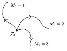
Figure 1: Flows of the free energy ${\cal F}_{0}$

in which $c$ as well as $g_{0}$ are different depending on the case. ( $g_{0}$ is the “gauge” freedom to be fixed arbitrarily, except for case i)). Then these branch points move through deformation of $\tau$ as given by the hodograpgh solution (5). The curve might happen to degenerate at some flow points $\vec{T}\neq 0$. We may expect a large variety of degeneracy of the $N=1^{*}$ theory, depending on the choice of $c$, though the free energy is initially the same.

8 Interpretation of the flow parameters $\Lambda_{M}$

We shall give a physical interpretation of the flow parameters $\Lambda_{M}$ which are so far mathematical. Namely we will show that the free energy (13) in the small phase space is equivalent to the one of the matrix model given by

$$Z=\int d\Phi{e^{-NtrV(\Phi)}\over det([\Phi,-]+i)},$$ (1)

with

$$V(\Phi)=\sum_{M=0}^{M_{0}}\bar{\Lambda}_{M}\Phi^{2M}.$$

Here $\Phi$ is an $N\times N$ hermite matrix and $\bar{\Lambda}_{M}$ is a linear combination of $\Lambda_{M}$ which will be given later. It can be done by making use of the arguments in [3]. Namely they discussed the relation between the Toda hierarchy and a matrix model. The matrix model (1) is its variant and was studied in [2, 12, 16]. There underlies the KdV hierarchy. So we shall adapt the arguments in [3] to this case. By diagonalizing $\Phi$ the integral (1) is reduced to an integral over the eigenvalues $\lambda_{1},\lambda_{2},\cdots,\lambda_{N}$. Then we obtain the saddle point equation

$$-NV^{\prime}(\lambda_{I})+\sum_{J\neq I}[{2\over\lambda_{I}-\lambda_{J}}-{1\over\lambda_{I}-\lambda_{J}+i}-{1\over\lambda_{I}-\lambda_{J}-i}]=0.$$ (2)

Let us take the large $N$ limit and assume that the eigenvalues spread out along the real line $[-\alpha,\alpha]$ with the density $\rho(\lambda)$. The integral (1) is written in the form

$$\log Z = -N^{2}\{\int_{-\alpha}^{\alpha}d\lambda\rho(\lambda)V(\lambda)-{1\over 2}\int_{-\alpha}^{\alpha}d\lambda\rho(\lambda)\int_{-\alpha}^{\alpha}d\lambda^{\prime}\rho(\lambda^{\prime})$$ (3)

$$\cdot[2\log(\lambda-\lambda^{\prime})-\log(\lambda-\lambda^{\prime}+i)-\log(\lambda-\lambda^{\prime}-i)]\}.$$

and (2) becomes

$$V^{\prime}(\lambda)-\int_{-\alpha}^{\alpha}d\lambda^{\prime}\rho(\lambda^{\prime})[{2\over\lambda-\lambda^{\prime}}-{1\over\lambda-\lambda^{\prime}+i}-{1\over\lambda-\lambda^{\prime}-i}]=0,$$ (4)

for $\lambda\in[-\alpha,\alpha]$. The l.h.s. of this equation is a force acting on a test eigenvalue $\lambda$. Introducing the resolvent

$$\omega(\lambda)=\int_{-\alpha}^{\alpha}d\lambda^{\prime}{\rho(\lambda^{\prime})\over\lambda-\lambda^{\prime}},$$

we rewrite this force as

$$f(\lambda)\equiv V^{\prime}(\lambda)\ -\ [2\omega(\lambda)\ -\ \omega(\lambda+i)\ -\ \omega(\lambda-i)].$$ (5)

Then the saddle point equation (4) reads

$$f(\lambda)=0,\quad\quad\quad{\rm for}\quad\lambda\in[-\alpha,\alpha].$$ (6)

We further introduce the function

$$G(\lambda)=U(\lambda)+i[\omega(\lambda+{i\over 2})-\omega(\lambda-{i\over 2})],$$ (7)

with a polynomial $U(\lambda)$ such that

$$V^{\prime}(\lambda)=-i[U(\lambda+{i\over 2})-U(\lambda-{i\over 2})].$$ (8)

To be concrete, $U(\lambda)$ is found in the form

$${\partial U(\lambda)\over\partial\bar{\Lambda}_{M}}=\sum_{k=0}^{M}c_{k}^{(M)}\lambda^{2k},\quad\quad\quad c_{M}^{(M)}=1,$$ (9)

in which $c_{k}^{(M)}$ are numerical values recursively determined with the requirement (8). In terms of the function $G(\lambda)$ the saddle point equation (6) becomes

$$G(\lambda+{i\over 2})=G(\lambda-{i\over 2}),\quad\quad\quad{\rm for}\quad\lambda\in[-\alpha,\alpha].$$ (10)

This function has two branch cuts along

$${\cal C}_{+}=[-\alpha+{i\over 2},\alpha+{i\over 2}],\quad\quad\quad\quad{\cal C}_{-}=[-\alpha-{i\over 2},\alpha-{i\over 2}].$$

The saddle point equation (10) implies that $G(\lambda)d\lambda$ is a meromorphic differential on an elliptic curve with the pole structure read in (7). We take $A$-cycle and the dual $B$-cycle in the same way as in [2]. We also define the function $\xi(\lambda)$ by integrating the force (5):

$$\xi(\lambda) \equiv \int_{\infty}^{\lambda}d\lambda f(\lambda)$$

$$= V(\lambda)-\int_{-\alpha}^{\alpha}d\lambda^{\prime}\rho(\lambda^{\prime})[2\log(\lambda-\lambda^{\prime})-\log(\lambda-\lambda^{\prime}+i)-\log(\lambda-\lambda^{\prime}-i)].$$

It is known [2] that for $\lambda\in[-\alpha,\alpha]$ this function is $\lambda$-independent as

$$\xi(\lambda)=\int_{\infty}^{\alpha}d\lambda f(\lambda)=i\oint_{B}d\lambda G(\lambda).$$ (12)

Noting that the jump in $G(\lambda)$ along the branch cut ${\cal C}_{+}$ (going upwards ) is $2\pi\rho(\lambda)$, we rewrite the free energy (3) as

$$\log Z = -N^{2}\{{1\over 2}\oint_{A}{d\lambda\over 2\pi}G(\lambda)V(\lambda)\ -\ {1\over 8}\oint_{A}{d\lambda\over 2\pi}\oint_{A}{d\lambda^{\prime}\over 2\pi}G(\lambda)G(\lambda^{\prime})$$ (13)

$$\cdot[2\log(\lambda-\lambda^{\prime})-\log(\lambda-\lambda^{\prime}+i)-\log(\lambda-\lambda^{\prime}-i)]\}.$$

Let us define the variable $\bar{a}$ by

$$\bar{a}=\oint_{A}G(\lambda)d\lambda.$$ (14)

We differentiate the free energy (13) by this $\bar{a}$:

$${\partial\log Z\over\partial\bar{a}}=-{N^{2}\over 2}\oint_{A}{d\lambda\over 2\pi}{\partial G(\lambda)\over\partial\bar{a}}\xi(\lambda).$$

Remember the fact that $\xi(\lambda)$ is $\lambda$-independent on the $A$-cycle and written as (12). Then this becomes

$${\partial\log Z\over\partial\bar{a}} = -i{N^{2}\over 2}\oint_{A}{d\lambda\over 2\pi}{\partial G(\lambda)\over\partial\bar{a}}\oint_{B}d\lambda G(\lambda)$$ (15)

$$= -i{N^{2}\over 4\pi}\oint_{B}d\lambda G(\lambda),$$

due to (14). By a similar calculation we have

$${\partial\log Z\over\partial\bar{\Lambda}_{M}}=-N^{2}[{1\over 2}\oint_{A}{d\lambda\over 2\pi}{\partial G(\lambda)\over\partial\bar{\Lambda}_{M}}\xi(\lambda)+{1\over 2}\oint_{A}{d\lambda\over 2\pi}G(\lambda){\partial V(\lambda)\over\partial\bar{\Lambda}_{M}}].$$ (16)

Use ${\partial\bar{a}\over\partial\bar{\Lambda}_{M}}=0$ and the properties of $\xi(\lambda)$ again. It may be written as

$${\partial\log Z\over\partial\bar{\Lambda}_{M}}=-i{N^{2}\over 2}\oint_{A}{d\lambda\over 2\pi}G(\lambda)\oint_{B}d\lambda{\partial G(\lambda)\over\partial\bar{\Lambda}_{M}}.$$ (17)

Finally we have recourse to the Riemann bilinear formula to proceed the calculation. Knowing the singular behavior of ${\partial G(\lambda)\over\partial\bar{\Lambda}_{M}}$ from (9) we obtain

$${\partial\log Z\over\partial\bar{\Lambda}_{M}}=i{N^{2}\over 4\pi}\sum_{k=0}^{M}2\pi i\ c_{k}^{(M)}{\rm res}_{\lambda=\infty}[{\scriptstyle{\lambda^{2k+1}}\over{\scriptstyle{2k+1}}}G(\lambda)d\lambda].$$ (18)

We think of the mapping from the $\lambda$-plane to the $z$-plane parameterizing the torus with the period ${\omega_{2}\over\omega_{1}}$. In [16] it was given by

$$\lambda(z)=-{\omega_{1}\over\pi}[\zeta(z)-{\zeta(\omega_{1})\over\omega_{1}}z]=-{\omega_{1}\over\pi}[{1\over z}+O(z)].$$ (19)

with $\zeta(z)$ the Weierstrass $\zeta$-function. By using this coordinate $z$ (18) becomes

$${\partial\log Z\over\partial\bar{\Lambda}_{M}}=-i{N^{2}\over 4\pi}\sum_{k=0}^{M}2\pi i\ c_{k}^{(M)}({\omega_{1}\over\pi})^{2k+1}{\rm res}_{z=0}[{\scriptstyle{z^{-2k-1}}\over{\scriptstyle{2k+1}}}G(\lambda)d\lambda].$$ (20)

If we can identify the meromorphic differential $G(\lambda)d\lambda$ with $dS$ and $\log Z$ with $-i{\cal F}_{0}$, then (15) and (18) become the equations (12) and (13) by appropriate linear combination of $\bar{\Lambda}_{M}$. Thus we can interpret the flow parameters $\Lambda_{M}$ of the Whitham deformation as the coupling constants $\bar{\Lambda}_{M}$ of the matrix model (1). So we are left with the task to show $G(\lambda)d\lambda$ to take the same form as (9). To this end we write the elliptic curve (1) in the form

$$y^{2}=4t^{3}-g_{2}\,t-g_{3},$$ (21)

and note that it is mapped to the $z$-plane through the Weierstrass ${\cal P}$-function

$$t=-\zeta^{\prime}(z)={\cal P}(z),\quad\quad\quad y={\cal P}^{\prime}(z).$$ (22)

Following [16] we shall determine the elliptic function $G(\lambda)$. From (7), (9) and (19) we know the pole singularity

$$[G(\lambda(z))]_{-}=\sum_{M=0}^{M_{0}}\bar{\Lambda}_{M}\sum_{k=0}^{M}c_{k}^{(M)}({\omega_{1}\over\pi})^{2k}\sum_{i=0}^{k}d_{i}^{(k)}z^{-2i},$$ (23)

in which $[\cdots]_{-}$ indicates the part of non-positive powers in $z$ and $d_{i}^{(k)}$ are calculable constants with $d_{k}^{(k)}=1$. By using the expansion

$${\cal P}(z)={1\over z^{2}}+{g_{2}\over 20}z^{2}+{g_{3}\over 28}z^{4}+\cdots,$$ (24)

it may be expressed by a polynomial of ${\cal P}(z)$ That is,

$$[G(\lambda(z))]_{-} = \sum_{M=0}^{M_{0}}\bar{\Lambda}_{M}\sum_{k=0}^{M}c_{k}^{(M)}({\omega_{1}\over\pi})^{2k}[{\cal P}(z)^{k}+d_{k-1}^{(k)}{\cal P}(z)^{k-1}+\cdots]_{-}$$ (25)

$$\equiv [\sum_{M=0}^{M_{0}}\bar{\Lambda}_{M}\sum_{k=0}^{M}c_{k}^{(M)}({\omega_{1}\over\pi})^{2k}\bar{P}_{k}({\cal P}(z))]_{-},$$

with a polynomial $\bar{P}_{k}(\cdot)$ of degree $k$. Since an elliptic function is determined uniquely by the pole singularity, so that

$$G(\lambda(z))=\sum_{M=0}^{M_{0}}\bar{\Lambda}_{M}\sum_{k=0}^{M}c_{k}^{(M)}({\omega_{1}\over\pi})^{2k}\bar{P}_{k}({\cal P}(z)).$$ (26)

By means of (19), (22) and (26) the meromorphic differential $G(\lambda)d\lambda$ can be written as

$$G(\lambda)d\lambda=\sum_{M=0}^{M_{0}}\bar{\Lambda}_{M}\sum_{k=0}^{M}c_{k}^{(M)}({\omega_{1}\over\pi})^{2k+1}[t+{\zeta(\omega_{1})\over\omega_{1}}]\bar{P}_{k}(t){dt\over y}.$$ (27)

By a linear transformation from $\bar{\Lambda}_{M}$ to $\Lambda_{M}$ this takes the form (9), except for the boundary term in $d\tilde{\Omega}_{M}$ which vanishes at $t=\infty$. But, when we interpreted the saddle point equation (10), we could allow $G(\lambda)d\lambda$ to have a boundary term like $d(\cdots)$ which is not meromorphic. As long as it vanishes at $\lambda=\infty$, the argument thereafter goes through without any modification. Appropriately fixing this freedom would yield the boundary term in $dS$. Or note that this boundary term depends on the gauge fixing discussed in Section 3. Then we can simply say that $\log Z$ of the matrix model corresponds to the free energy ${\cal F}_{0}$ of the Whitham hierarchy calculated with the particular gauge in which the boundary term disappears, for instance, $v=const$ and $w=const$.

Thus we were able to identify the free energy (13) in the small phase space with the one of the matrix model (1). The free energy (12) in the large phase space may be identified as the one obtained by peturbing the model (1):

$$Z=\int d\Phi\ {e^{-Ntr[\sum_{M=0}^{M_{0}}\bar{\Lambda}_{M}\Phi^{2M}-\sum_{M=0}^{\infty}\bar{T}_{M}\Phi^{2M}]}\over det(\ [\Phi,-]\ \ +\ \ i\ )\ }.$$ (28)

In section 5 we have shown how to obtain the free energy (12) by perturbing the one (13) in the small phase space. We can obtain the free energy of the model (28) by perturbing the model (1) exactly in the same sense. Thus the flow parameters $T_{M},M=1,2,\cdots$ of the free energy (12) in the large phase space can be interpreted as the coupling constants $\bar{T}_{M}$ of the perturbative interaction of the matrix model (28).

The different characterizations of the free energy by (20), (24) and (28) in the previous section corresponds to the matrix model (1) with $M_{0}=0,1,2$ after an appropriate setting of $\bar{\Lambda}_{M}$. The three flows illustrated in Fig. 1 are interpreted as different perturbations of these matrix models by (28). Then (32) or more concretely (36) is interpreted as a condition which sets the free energy $\log Z$ with $M_{0}=0,1,2$ to be equal at $\bar{T}_{M}=0$. It can be done by choosing the period $\tau={\omega_{2}\over\omega_{1}}$ of the torus appropriately.

We have discussed only the $two$-cut solution of the matrix model (1). We may consider multi-cut solutions on a Riemann surface with higher genus. It would be interesting to extend the whole arguments in this section to such general cases.

9 Conclusions

In this paper we have discussed the Whitham deformation of the free energy ${\cal F}_{0}$ which appears in the DV and SW theories. It amounts to discussing deformation of a relevant (hyper)elliptic curve with flow parameters. We were mainly concerned about the elliptic case. Generalization to the hyperelliptic case would be straightforward albeit with some technical complications. We then derived the Whitham equation for the period $\tau$. Its hodograph solution represents the Whitham deformation of the free energy ${\cal F}_{0}$ in the large phase space of flow parameters. To find a hodograph solution we have to impose a constraint which determines an initial functional form $\tau_{0}(a)$ or $a(\tau_{0})(\equiv\tau_{0}^{-1}(a))$. It amounts to determining the free energy ${\cal F}_{0}$ in the small phase space. The main message of this paper is that $\tau_{0}(a)$ and ${\cal F}_{0}$, given at one point in the small phase space, get deformed along different flows in the large phase space, when the elliptic curve is parameterized differently at that point. As an application of this argument we took the effective superpotential of the $N=1^{*}$ theory (7). We have shown that the same superpotential can be indeed characterized by the DV differentials (20), (24) and (28) on different curves. For each chosen DV differential the superpotential undergoes different Whitham deformations. We have also given an interpretation of these Whitham deformations in terms of the matrix model.

The free energy ${\cal F}_{0}$ of the $N=1^{*}$ theory took rather complicated forms for each case of i), ii) and iii). We emphasize that the term $\int^{\tau}d\tau(...)$ coming from the boundary term in (4) is essential to have the property $\tau={\partial^{2}{\cal F}_{0}\over\partial a^{2}}$. If two of the branch points of the curve are fixed to be constant, for instance, $v=1$ and $w=-1$ as in the $N=2$ effective Yang-Mills theory in Subsection 7.1, there is no contribution from the boundary. In such cases the free energy ${\cal F}_{0}$ is rather simply calculated. But in general the boundary term was necessary for the compatibility of the Whitham deformation (2) and (3).

The arguments in this paper can be applied for the SW theory in which the constraint (4) is inverted to give the initial condition

$$\tau_{0}(a)={g_{D0}\over g_{0}}\sim const.+{i\over\pi}\log a^{2},\quad\quad\quad a\sim\infty,$$ (1)

by using (1) and (2). This condition is essentially related to the effective coupling $g_{eff}$ of QCD. We might parameterize the elliptic curve in the general form (1) and realize the initial constraint (1) by the generalized differential (9) with $M_{0}\geq 2$. Then $a$ is expressed by the branch pints $u,v$ and $w$. They move obeying the Whitham equation. We might think of the Whitham equation as a master equation for studying degeneration of the curve, that is, critical phenomena of QCD.

Appendix A The Weierstrass standard form and the period integrals

We write an elliptic curve in the Weierstrass standard form

$$y^{2}=4(t-e_{1})(t-e_{2})(t-e_{3})$$ (1)

with

$$e_{1}+e_{2}+e_{3}=0.$$

Then the Jacobi $\theta$-functions are given in terms of the positions of the branch points $e_{1},e_{2}$ and $e_{3}$:

$$\theta_{2}(\tau) = \sum_{n=-\infty}^{\infty}q^{{1\over 2}(n-{1\over 2})^{2}}=i\left({2\omega_{1}\over\pi}\right)^{1\over 2}(e_{2}-e_{3})^{1\over 4},$$

$$\theta_{3}(\tau) = \sum_{n=-\infty}^{\infty}q^{{1\over 2}n^{2}}=\left({2\omega_{1}\over\pi}\right)^{1\over 2}(e_{1}-e_{3})^{1\over 4},$$ (2)

$$\theta_{4}(\tau) = \sum_{n=-\infty}^{\infty}(-1)^{n}q^{{1\over 2}n^{2}}=\left({2\omega_{1}\over\pi}\right)^{1\over 2}(e_{1}-e_{2})^{1\over 4},$$

with

$$q = e^{2\pi i\tau},$$

$$\omega_{1} = \int_{-\infty}^{e_{1}}{dt\over\sqrt{4(t-e_{1})(t-e_{2})(t-e_{3})}}.$$

(1) may be also written in the form

$$y^{2}=4t^{3}-g_{2}t-g_{3}.$$ (3)

It is known that the coefficients are given by the Eisenstein series

$$g_{2} = 2(e_{1}^{2}+e_{2}^{2}+e_{3}^{2})$$ (4)

$$= {4\over 3}({\pi\over g_{0}})^{4}[1+240\sum_{n=1}^{\infty}{n^{3}q^{n}\over 1-q^{n}}]\equiv{4\over 3}({\pi\over g_{0}})^{4}E_{4}(\tau),$$

$$g_{3} = 4e_{1}e_{2}e_{3}$$ (5)

$$= {8\over 27}({\pi\over g_{0}})^{6}[1-504\sum_{n=1}^{\infty}{n^{5}q^{n}\over 1-q^{n}}]\equiv{8\over 27}({\pi\over g_{0}})^{6}E_{6}(\tau).$$

with $g_{0}=\oint_{A}{dt\over y}=-2\omega_{1}$. By using them we have the following integration formulae

$${1\over g_{0}}\oint_{A}t{dt\over y} = g_{1},\quad\quad\quad\quad\quad\quad{1\over g_{0}}\oint_{B}t{dt\over y}=-\tau g_{1}+{2\pi i\over g_{0}^{2}},$$ (6)

$${1\over g_{0}}\oint_{A}t^{2}{dt\over y} = {g_{2}\over 12},\quad\quad\quad\quad\quad\quad\quad\quad{1\over g_{0}}\oint_{B}t^{2}{dt\over y}=\tau{g_{2}\over 12},$$ (7)

$${1\over g_{0}}\oint_{A}t^{3}{dt\over y} = {3\over 20}g_{2}g_{1}+{g_{3}\over 10},\quad\quad{1\over g_{0}}\oint_{B}t^{3}{dt\over y}=\tau[{3\over 20}g_{2}g_{1}+{g_{3}\over 10}],$$ (8)

Here $g_{1}$ is also given by the Eisenstein series:

$$g_{1}={1\over 3}({\pi\over g_{0}})^{2}[1-24\sum_{n=1}^{\infty}{nq^{n}\over 1-q^{n}}]\equiv-{1\over 3}({\pi\over g_{0}})^{2}E_{2}(\tau).$$ (9)

(7) and (8) can be easily shown from

$$\oint d(y)=0,\quad\quad\quad\oint d(ty)=0.$$

Appendix B Calculations of $d\Omega_{M}$ and $\tau_{MN}$

We will obtain a formula for the $2$-point function $\tau_{MN}$, directly calculating the residue of (11). First of all we expand $d\Omega_{N}$ given by (2) at $x={1\over\xi^{2}}=\infty$. Let the expansion of ${dx\over y}$ to be

$${dx\over y}=-\sum^{\infty}_{M=1}R_{M}\xi^{2M-2}d\xi,$$ (1)

in which

$$R_{1}=1,\quad\quad R_{2}={c\over 2},\quad\quad R_{3}={5c^{2}\over 24}+{1\over 8}g_{2},\hskip 28.45274pt$$

$$R_{4}={\ 35c^{3}\over 432}+{7c\over 48}g_{2}+{1\over 8}g_{3},$$

$$R_{5}={35c^{4}\over 1152}+{7c^{2}\over 64}g_{2}+{3c\over 16}g_{3}+{3\over 128}(g_{2})^{2},$$

$$R_{6}={77c^{5}\over 6912}+{77c^{3}\over 1152}g_{2}+{11c^{2}\over 64}g_{3}+{11c\over 256}(g_{2})^{2}+{3\over 64}g_{3}g_{2},$$

$$\hskip 28.45274pt\quad{\it etc},$$

with $c$ defined by (2). Then the requirement (8) gives the relation

$${}^{t}(\gamma_{N-1}\gamma_{N-2}\cdots\cdots\gamma_{1})=-{\cal K}^{-1}{}^{t}(R_{2}\cdots\cdots R_{N}),\quad\quad N\geq 2$$ (3)

with the matrix ${\cal K}$

$${\cal K}=\left(\begin{array}[]{ccccc}R_{1}&&&&\smash{\lower 7.3194pt\hbox{\bg 0}}\\ R_{2}&R_{1}&&&\\ \vdots&\vdots&&\ddots&\\ R_{N-1}&R_{N-2}&\cdot&\cdot&R_{1}\end{array}\right).$$ (8)

By (2) and (3), (11) is calculated as

$${\scriptstyle{2M-1}\over\scriptstyle{2\pi i}}\tau_{NM} = -{\rm res}_{\xi=0}[\xi^{-2M+1}d\Omega_{N}]$$ (9)

$$= R_{M+N}+\gamma_{0}R_{M}$$

$$\quad-(R_{M+N-1}\cdots\cdots R_{M+1}){\cal K}^{-1}{}^{t}(R_{2}\cdots\cdots R_{N}),$$

for $N\geq 2$ and $M\geq 1$. Here $\gamma_{0}$ is the constant in $d\Omega_{N}$ which is determined by (7). For $N=1$ and $M\geq 1$ we have

$${\scriptstyle{2M-1}\over\scriptstyle{2\pi i}}\tau_{1M} = -{\rm res}_{\xi=0}[\xi^{-2M+1}d\Omega_{1}]$$ (10)

$$= R_{M+1}-(g_{1}+{c\over 3})R_{M},$$

in which $g_{1}$ was given by (9). From $\tau_{1N}=\tau_{N1}$ we find alternatively $\gamma_{0}$ in (9) to be

$$\gamma_{0} = -{2N-2\over 2N-1}R_{N+1}-{1\over 2N-1}(g_{1}+{c\over 3})R_{N}$$ (11)

$$\hskip 28.45274pt+(R_{N}\cdots\cdots R_{2}){\cal K}^{-1}{}^{t}(R_{2}\cdots\cdots R_{N}).,\quad\quad N=2,3,\cdots.$$

For $\tau_{0N}$ with $M\geq 1$ we have

$${\scriptstyle{2M-1}\over\scriptstyle{2\pi i}}\tau_{0M}\equiv{\scriptstyle{2M-1}\over\scriptstyle{2\pi i}}\tau_{M0}={R_{M}\over g_{0}},$$ (12)

from (9) and (10). Evaluating the formulae (9), (10) and (12) for simple cases yields $\tau_{AB}(=\tau_{BA})$ with $A,B=0,1,2,\cdots$, as

$$\tau_{01} = {2\pi i\over g_{0}},\quad\quad\tau_{02}={2\pi i\over g_{0}}{c\over 6},\quad\quad\tau_{03}={2\pi i\over g_{0}}[{c^{2}\over 24}+{g_{2}\over 40}],$$

$$\tau_{11} = 2\pi i[{c\over 6}-g_{1}],$$

$$\tau_{12} = 2\pi i[{c^{2}\over 72}-{c\over 6}g_{1}+{g_{2}\over 24}],$$

$$\tau_{13} = 2\pi i[{13c^{3}\over 432}+{c^{2}\over 24}g_{1}+{3c\over 80}g_{2}+{g_{3}\over 40}+{g_{1}g_{2}\over 40}],$$ (13)

$$\tau_{22} = \pi i[{c^{3}\over 324}-{c^{2}\over 18}g_{1}+{c\over 36}g_{2}+{1\over 12}g_{3}],$$

$$\tau_{23} = \pi i[{c^{4}\over 1728}-{c^{3}\over 72}g_{1}+{c^{2}\over 96}g_{2}+{c\over 20}(g_{3}-{g_{1}g_{2}\over 6})+{(g_{2})^{2}\over 192}],$$

$$\tau_{33} = \pi i[{c^{5}\over 8640}-{c^{4}\over 288}g_{1}+{c^{3}\over 288}g_{2}+{c^{2}\over 240}(-g_{2}g_{1}+6g_{3})$$

$$\hskip 28.45274pt+{c\over 192}(g_{2})^{2}+{3\over 400}g_{3}g_{2}-{1\over 800}(g_{2})^{2}g_{1}].$$

Appendix C Consistency check

We shall alternatively check that (12) and (32) follow from from (13), although they are proved by (11) together with (10) and the calculation (7.2) respectively. It gives an independent consistency check of our formalism for the Whitham hierarchy.

C.1 Check of (7.12)

To this end we have to explicitly evaluate $s_{M}(\tau)$, given by (5). Let us put it in the form

$$s_{M}(\tau)=g_{0}{\Gamma_{M}\over\Gamma_{0}},\quad\quad M=1,2,\cdots,$$ (1)

with

$$\Gamma_{M}=u^{\prime}Q_{M}(u)(v-w)+v^{\prime}Q_{M}(v)(w-u)+w^{\prime}Q(w)_{M}(u-v).$$ (2)

Writing the curve (1) in the Weierstrass standard form (1) we have

$$u(\tau)=e_{1}+{c\over 3},\quad\quad v(\tau)=e_{2}+{c\over 3},\quad\quad w(\tau)=e_{3}+{c\over 3}.$$ (3)

Then (2) reads

$$\Gamma_{M}=(e_{1}^{\prime}+{c^{\prime}\over 3})Q_{M}(e_{1}+{c\over 3})(e_{2}-e_{3})+cyclic.$$ (4)

First of all we replace $e_{i}^{\prime}(={\partial e_{i}\over\partial\tau})$ in (4) by

$${1\over 2\pi i}e_{i}^{\prime}=-{1\over 2}({g_{0}\over\pi})^{2}(e_{i}^{2}+g_{1}e_{i}-{g_{2}\over 6})-{1\over\pi i}{g_{0}^{\prime}\over g_{0}}e_{i},$$ (5)

which is a variant of the formula due to Itoyama and Morosov[7]

$$2{\partial\over\partial\log q}\hat{e}_{i}={1\over 6}\hat{g}_{2}(\tau)-\hat{g}_{1}(\tau)\hat{e}_{i}-\hat{e}_{i}^{2},\quad\quad\quad q=e^{2\pi i\tau},$$ (6)

with

$$\hat{e}_{i} = ({g_{0}\over\pi})^{2}e_{i},$$

$$\hat{g}_{1}(\tau) = -{1\over 3}E_{2}(\tau)=({g_{0}\over\pi})^{2}g_{1},$$

$$\hat{g}_{2}(\tau) = {2\over 3}[\theta_{2}(\tau)^{8}+\theta_{3}(\tau)^{8}+\theta_{0}(\tau)^{8}]$$

$$= {4\over 3}E_{4}(\tau)=({g_{0}\over\pi})^{4}g_{2}.$$

Here $g_{1}$ and $g_{2}$ are given by (9) and (4). Then we find

$${1\over 2\pi i}\Gamma_{M} = [-{1\over 2}({g_{0}\over\pi})^{2}(e_{1}^{2}+g_{1}e_{1}-{g_{2}\over 6})-{1\over\pi i}{g_{0}^{\prime}\over g_{0}}e_{1}+{1\over 2\pi i}{c^{\prime}\over 3}]Q_{M}(e_{1}+{c\over 3})(e_{2}-e_{3})$$ (7)

$$\hskip 28.45274pt+cyclic.$$

Next we replace $Q_{M}(e_{i}+{c\over 3}),i=1,2,3$, in the r.h.s. by those calculated in (20), (24) and (28). The resultant $\Gamma_{M}$ is simplified by the formulae

$${1\over 2}({g_{0}\over\pi})^{2}e_{1}^{2}(e_{2}-e_{3})+cyclic = -{\Gamma_{0}\over 2\pi i},$$ (8)

$${1\over 2}({g_{0}\over\pi})^{2}e_{1}^{3}(e_{2}-e_{3})+cyclic = 0,$$ (9)

$${1\over 2}({g_{0}\over\pi})^{2}e_{1}^{4}(e_{2}-e_{3})+cyclic = -{\Gamma_{0}\over 2\pi i}{g_{2}\over 4},$$ (10)

$${1\over 2}({g_{0}\over\pi})^{2}e_{1}^{5}(e_{2}-e_{3})+cyclic = -{\Gamma_{0}\over 2\pi i}{g_{3}\over 4},$$ (11)

$${1\over 2}({g_{0}\over\pi})^{2}e_{1}^{6}(e_{2}-e_{3})+cyclic = -{\Gamma_{0}\over 2\pi i}({1\over 16}(g_{2})^{2}+{1\over 2}g_{1}g_{3}),$$ (12)

$$\cdots\cdots$$

Finally we eliminate $c^{\prime}(={\partial c\over\partial\tau})$ from $\Gamma_{M}$ for the cases with $M_{0}=1,M_{0}=2$ and $M_{0}=3$ by means of the constraints (17)$\sim$(19) respectively. To this end we need to differentiate the constraints by $\tau$ using the formulae

$${\partial\over\partial\tau}E_{2}(\tau) = {i\pi\over 6}(E_{2}(\tau)^{2}-E_{4}(\tau)),$$ (13)

$${\partial\over\partial\tau}E_{4}(\tau) = {2\pi i\over 3}(E_{2}(\tau)E_{4}-E_{6}(\tau)),$$ (14)

$${\partial\over\partial\tau}E_{6}(\tau) = -i\pi(E_{4}(\tau)^{2}-E_{2}(\tau)E_{6}(\tau)),$$

$$\cdots\cdots.$$

We have checked that the characteristic speeds (1) with $\Gamma_{M}$ thus evaluated indeed satisfy (12) for the respective case of $M_{0}=1,M_{0}=2$ and $M_{0}=3$.

The formulae (8)$\sim$(12), (13)$\sim$(C.1) can be shown by means of (5). First of all we show (8)$\sim$(12). Integrating (9) along a $A$-cycle in the Weierstrass standard form we obtain

$$\oint_{A}{1\over t-e_{1}}{dt\over y}={g_{0}\over\Gamma_{0}}(e_{2}^{\prime}-e_{3}^{\prime})+2{e_{2}-e_{3}\over\Gamma_{0}}g_{0}^{\prime}.$$

By means of (5) it becomes

$${1\over 2\pi i}\oint_{A}{1\over t-e_{1}}{dt\over y}={1\over 2}({g_{0}\over\pi})^{2}{g_{0}\over\Gamma_{0}}(e_{2}-e_{3})(e_{1}-g_{1}).$$ (16)

The similar formulae are found by cyclic rotation of $e_{1}$, $e_{2}$ and $e_{3}$. Now we calculate $d({t^{n}\over y})$ for $n=1,2,3,4,5$ as

$$d({t\over y})=[-{1\over 2}-{1\over 2}\sum_{i}{e_{i}\over t-e_{i}}]{dt\over y},\hskip 56.9055pt$$

$$d({t^{2}\over y})=[{t\over 2}-{1\over 2}\sum_{i}{e_{i}^{2}\over t-e_{i}}]{dt\over y}.\hskip 56.9055pt$$

$$\hskip 28.45274pt\cdots\cdots\cdots\cdots$$

Integrate them along a $A$-cycle and use (16). With (4)$\sim$(9) we then obtain the formulae (8)$\sim$(12).

Next we go to the proof of (13)$\sim$(C.1). Either of them is proved similarly. We will sketch a proof of (14). Differentiate the first equation of (7) by $\tau$:

$$({g_{2}\over 12})^{\prime}=-{g_{0}^{\prime}\over g_{0}}{g_{2}\over 12}+{1\over 2g_{0}}\sum_{i}e_{i}^{\prime}\oint_{A}[t+e_{i}+{e_{i}^{2}\over t-e_{i}}]{dt\over y}.$$ (17)

We calculate the second piece of the r.h.s. by the following three steps: At first perform the integration by (6)$\sim$(8) and (16). Next replace $e_{i}^{\prime}$ by the formula (5). Finally sum over $i$ by (8)$\sim$(11). Then we find

$${1\over 2g_{0}}\sum_{i}e_{i}^{\prime}\oint_{A}[t+e_{i}+{e_{i}^{2}\over t-e_{i}}]{dt\over y}\ =\ -{\pi i\over 2}({g_{0}\over\pi})^{2}[{g_{3}\over 2}+{g_{1}g_{2}\over 3}]-{g_{0}^{\prime}\over g_{0}}{g_{2}\over 4}.$$ (18)

On the other hand the l.h.s. of (17) is calculated as

$$({g_{2}\over 12})^{\prime}=-{g_{0}^{\prime}\over g_{0}}{g_{2}\over 3}+{1\over 9}({\pi\over g_{0}})^{4}E_{4}(\tau)^{\prime},$$ (19)

by (4). Putting (18) and (19) into (17) and using the Eisenstein series, we obtain (14).

C.2 Check of (7.32)

We check (32) for case ii), i.e.,

$$\Lambda_{2}^{2}{\partial\over\partial\tau}\tilde{\tau}_{22}=[{\pi\over 72}(E_{2}(\tau)^{2}-E_{4}(\tau))]^{2}.$$ (20)

For other cases it can be done similarly. In the first place we compute the residue in $\tilde{\tau}_{22}$ given by (26):

$$2\pi i\ {\rm res}_{\xi=0}[\xi^{-4}d\xi\Delta_{2}(x,\tau)]$$

$$= \pi i[-{1\over\Gamma_{0}}\{Q_{2}(u)u^{\prime}(v^{\prime}w-w^{\prime}v)+cyclic\}+{c\over 2\Gamma_{0}}\{Q_{2}(u)u^{\prime}(v^{\prime}-w^{\prime})+cyclic\}],$$

using (6) and (1). By (3) both cyclic sums can be written as

$$Q_{2} (u) u^{\prime}(v^{\prime}w-w^{\prime}v)+cyclic$$

$$= Q_{2}(e_{1}+{c\over 3})(e^{\prime}_{1}+{c^{\prime}\over 3})[(e_{2}^{\prime}e_{3}-e_{3}^{\prime}e_{2})+{c\over 3}(e_{2}^{\prime}-e_{3}^{\prime})-{c^{\prime}\over 3}(e_{2}-e_{3})],$$

$$Q_{2} (u) u^{\prime}(v^{\prime}-w^{\prime})+cyclic$$

$$= Q_{2}(e_{1}+{c\over 3})(e^{\prime}_{1}+{c^{\prime}\over 3})(e_{2}^{\prime}-e_{3}^{\prime}).$$

With recourse to (5) and (8)$\sim$(12) they are evaluated in the same way as $\Gamma_{M}$, (4). After tedious calculations we find that

$$2\pi i\ {\rm res}_{\xi=0} [\xi^{-4}d\xi\Delta_{2}(x,\tau)]$$ (22)

$$= (\pi i)^{2}({g_{0}\over\pi})^{2}[{g_{2}^{2}\over 72}+{g_{1}g_{3}\over 4}++c({g_{1}g_{2}\over 18}+{g_{3}\over 12})+c^{2}({g_{2}\over 432}-{(g_{1})^{2}\over 36})]$$

$$+2\pi i{g_{0}^{\prime}\over g_{0}}[{g_{3}\over 4}+{c\over 18}g_{2}-{c^{2}\over 18}g_{1}]+\pi ic^{\prime}[-{g_{2}\over 36}+{c\over 9}g_{1}-{c^{2}\over 108}]$$

$$-({\pi\over g_{0}})^{2}[{1\over 3}(c^{\prime}-c{g_{0}^{\prime}\over g_{0}})]^{2}.$$

On the other hand we calculate ${\partial\tau_{22}\over\partial\tau}$ by differentiating directly the formula given by (13). Then add the result to (22). It exactly cancels the first three terms of (22). We use the constraint (23) and (13) in the last term to obtain (20).

References

- [1] R. Dijkgraaf and C. Vafa, Matrix models, topological strings, and supersymmetric gauge theories, Nucl. Phys. B 644 (2002) 3 [hep-th/0206255]; On geometry and matrix models, Nucl. Phys. B 644 (2002) 21 [hep-th/0207106].
- [2] R. Dijkgraaf and C. Vafa, A perturbative window into non-perturbative physics, [hep-th/0208048].
- [3] L. Chekhov and A. Mirnov, Matrix models vs. Seiberg-Witten/Whitham theories, Phys. Lett. B 552 (2003) 293 [hep-th/0209085].
- [4] H. Itoyama and A. Morosov, Dijkgraaf-Vafa prepotential in the context of general Seiberg-Witten theory, Nucl. Phys. B 657 (2003) 53 [hep-th/0211245]; Gluino -condensate(CIV-DV) prepotential from its Whitham derivatives, [hep-th/0301136]; L. Chekhov, A. Marshakov, A. Mirnov and D. Vasiliev, DV and WDVV, [hep-th/0301071]; M. Matone, Seiberg-Witten duality in Dijkgraaf-Vafa theory, Nucl. Phys. B 656 (2003) 78 [hep-th/0212253].
- [5] N. Seiberg and E. Witten, Electric-magnetic duality, monopole condensation, and confinement in supersymmetric Yang-Mills theory, Nucl. Phys. B 426 (1994) 19 [hep-th/9407087]; Monopoles, duality and chiral symmetry breaking in supersymmetric QCD, Nucl. Phys. B 431 (1994) 484 [hep-th/9408099].
- [6] A. Gorsky, I. Krichver, A. Marshakov, A. Mirnov and A. Morosov, Integrabilty and Seiberg-Witten exact solution, Phys. Lett. B 355 (1995) 466; E. Martinec and. N.P. Warner, Integrable systems and supersymmetric gauge theory, Nucl. Phys. B 459 (1996) 97 [hep-th/9509161]; T. Nakatsu and K. Takasaki, Whitham-Toda hierarchy and SUSY Yang-Mills theory, Mod. Phys. Lett. A 11 (1996) 157 [hep-th/9509162]; T. Eguchi and S.-K. Yang, Prepotentials of supersymmetric gauge theories and soliton equations, Mod. Phys. Lett. A 11 (1996) 131 [hep-th/9510183]; A. Gorsky, A. Marshakov, A. Mirnov and A. Morsov, WDVV-like equations in SUSY Yang-Mills theory, Phys. Lett. B 389 (1996) 43 [hep-th/9607109]; RG equations from Whitham hierarchy, Nucl. Phys. B 527 (1998) 690 [hep-th/9802007].
- [7] H. Itoyama and A. Morosov, Prepotential and the Seiberg-Witten theory, Nucl. Phys. B 491 (1997) 529 [hep-th/9512161].
- [8] M. Mario and G. Moore, The Donaldson-Witten function for gauge groups of rank larger than one, Commun. Math. Phys. 199 (1998) 423 [hep-th/9802185]; M. Mario, The uses of Whitham hierarchies, Prog. Theor. Phys. Suppl. 135 (1999) 29 [hep-th/9905053]; A. Losev, N. Nekrasov and S. Shatashvili, Issues in topological gauge theory, Nucl. Phys. B 534 (1998) 549 [hep-th/9711108]; K. Takasaki, Whitham deformations and tau functions in supersymmetric gauge theories, Prog. Theor. Phys. Suppl. 135 (1999) 53 [hep-th/9905224].
- [9] S. Novikov, S.V. Manakov, L.P. Pitaevskii and V.E. Zakharov, Theory of solitons: The inverse problem method, Plenum Press, New York 1984; A.V. Gurevich and L.P. Pitaevskii, Nonstationary structure of a collisionless shock wave, JETP 38 (1974) 291; H. Flaschka, M.G. Forest and D.W. McLaughlin, Multiphase averaging and inverse spectral solution of the Korteweg-de Vries equation, Commun. Pure Appl. Math. 33 (1980) 739; B.A. Dubrovin and S.P. Novikov, Hydrodynamics of weakly deformed soliton lattices. Differential geometry and Hamiltonian theory, Russian Math. Surveys 44:6 (1989) 35; A. M. Bloch and Y. Kodama, The Whitham equation and shocks in the Toda lattice in Singular limits of dispersive waves, Edited by N.M. Ercolani et al, Plenum Press, New York 1994.
- [10] R. Boels, J. de Boer, R. Duivenvoorden and J. Wijnhout, Nonperturbative superpotentials and compactification to three dimensions, hep-th/0304061; Factorization of Seiberg-Witten curves and compactification to three dimensions, [hep-th/0305189]; T.J. Hollowood, Critical points of glue ball superpotentials and equilibria of integrable systems, [hep-th/0305023].
- [11] Y. Kodama and Gibbons, A method for solving the dispersiomless KP hierarchy, Phys. Lett. A 135 (1989) 167.
- [12] R. Dijkgraaf, S. Gukov, V.A. Kazakov and C. Vafa, Perturbative analysis of gauged matrix models, [hep-th/0210238]. V.A. Kazakov, I.K. Kostov and N.A. Nekrasov, D-particles, matrix integrals and KP hierarchy, Nucl. Phys. B 557 (1999) 413 [hep-th/9810035].
- [13] R. Dijkgraaf and E. Witten, Mean field theory, topological field theory, and multi-matrix models, Nucl. Phys. B 342 (1990) 486; R. Dijkgraaf, H. Verlinde and E. Verlinde, Topological strings in , Nucl. Phys. B 352 (1991) 59.
- [14] T. Eguchi, Y. Yamada and S.-K. Yang, On the genus expansion in the topological string theory, Rev. Math. Phys. 7 (1995) 279 [hep-th/9405106]; B. Dubrovin, Geometry of 2d topological field theory, [hep-th/9407018].
- [15] S. Aoyama and Y. Kodama, Topological Landau-Ginzburg theory with a rational potential and the dispersionless KP hierarchy, Commun. Math. Phys. 196 (1996) 185 [hep-th/9505122].
- [16] N. Dorey, T.J. Hollowood, S.P. Kumar and A. Sinkovics, Exact superpotentials from matrix models, JHEP 0211 (2002) 039 [hep-th/0209089].