hep-th/0309230

Phase Structure of

Black Holes and Strings on Cylinders

Troels Harmark and Niels A. Obers

The Niels Bohr Institute

Blegdamsvej 17, 2100 Copenhagen Ø, Denmark

harmark@nbi.dk, obers@nbi.dk

Abstract

We use the $(M,n)$ phase diagram recently introduced in hep-th/0309116 to investigate the phase structure of black holes and strings on cylinders. We first prove that any static neutral black object on a cylinder can be put into an ansatz for the metric originally proposed in hep-th/0204047, generalizing a result of Wiseman. Using the ansatz, we then show that all branches of solutions obey the first law of thermodynamics and that any solution has an infinite number of copies. The consequences of these two results are analyzed. Based on the new insights and the known branches of solutions, we finally present an extensive discussion of the possible scenarios for the Gregory-Laflamme instability and the black hole/string transition.

1 Introduction

In [1] a new type of phase diagram for neutral and static black holes and black strings on cylinders $\mathbb{R}^{d-1}\times S^{1}$ was introduced. In this paper we continue to examine various aspects of the phase structure of black holes and strings on cylinders using this phase diagram. We furthermore establish new results that deepen our understanding of the phase structure.

The phase structure of neutral and static black holes and black strings on cylinders $\mathbb{R}^{d-1}\times S^{1}$ has proven to be very rich, but is also largely unknown. We can categorize the possible phase transitions into four types:

• Black string $\rightarrow$ black hole

• Black hole $\rightarrow$ black string

• Black string $\rightarrow$ black string

• Black hole $\rightarrow$ black hole

Since the event horizons of the black string and black hole have topologies $S^{d-2}\times S^{1}$ and $S^{d-1}$, respectively, we see that the first two types of phase transitions involve changing the topology of the horizon, while the last two do not.

Gregory and Laflamme [3, 4] discovered that light uniform black strings are classically unstable. In other words strings that are symmetric around the cylinder, are unstable to linear perturbations when the mass of the string is below a certain critical mass. This was interpreted to mean that a light uniform string decays to a black hole on a cylinder since that has higher entropy, thus being a transition of the first type above.

However, Horowitz and Maeda argued in [5] that the topology of the event horizon cannot change through a classical evolution. This means that the first two types of transitions above cannot happen through classical evolution. Therefore, Horowitz and Maeda conjectured that the decay of a light uniform string has an intermediate step: The light uniform string decays to a non-uniform string, which then eventually decays to a black hole. Thus, we first have a transition of the third type, then afterwards a transition from non-uniform black string to a black hole which is of the first type.

The conjecture of Horowitz and Maeda in [5] prompted a search for non-uniform black strings, and a branch of non-uniform string solutions was found in [7, 8]. However, this new branch of non-uniform string solutions was discovered to have lower entropy than uniform strings of the same mass, thus a given non-uniform string will decay to a uniform string (i.e. a process of the third type above).

If we consider black holes on a cylinder, it is clear that they cannot exist beyond a certain critical mass, since at some point the event horizon becomes too large to fit on a cylinder. Therefore, there should be a transition from large black holes to black strings, i.e. a transition of the second type above. However, it is not known how this transition precisely works.

Finally, as an example of a transition of the fourth type above, one can consider two black holes on a cylinder which are put opposite to each other. This configuration exists as a classical solution but it is unstable. Thus, the two black holes will decay to one black hole.

Several suggestions for the phase structure of the Gregory-Laflamme instability, the black hole/string transitions and the uniform/non-uniform string transitions have been put forward [5, 7, 10, 11, 12, 13, 14, 15] but it is unclear which of these, if any, are correct.

The outline of this paper is as follows. In Section 2 we collect the main results of [1]. We start by reviewing the two parameters of the new phase diagram, the mass $M$ and a new asymptotic quantity called the relative binding energy $n$. The plot of the known branches in the $(M,n)$ phase diagram is then given. We also recall the new Smarr formula of [1] and some of its consequences for the thermodynamics, as well as the Uniqueness Hypothesis.

In Section 3 we show that any static and neutral black hole or string on a cylinder can be put into the ansatz originally proposed in [10], generalizing the result of Wiseman [13] for $d=5$. This is done in two steps by first deriving the three-function conformal ansatz, and subsequently showing that one can transform to the two-function ansatz of [10]. The latter ansatz was shown to be completely determined by one function only, after explicitly solving the equations of motion. We then comment on the boundary conditions for this one function and their relation to the asymptotic quantities for black holes/strings on cylinders introduced in [1].

In Section 4 we use the ansatz of the previous section to prove that any curve of solutions always obeys the first law of thermodynamics

$$\delta M=T\delta S+nM\frac{\delta R_{T}}{R_{T}}\ .$$ (1.1)

Here the last term is due to the pressure in the periodic direction, and confirms the fact that $n$ is a meaningful physical quantity. Moreover, for fixed value of the circle radius $R_{T}$, this means that $\delta M=T\delta S$ for all solutions in the $(M,n)$ phase diagram. We analyze the consequences of this for the black hole/string phase transitions.

In Section 5 we further develop an argument of Horowitz [11] that a given non-uniform black string solution can be “unwrapped” to give a new non-uniform black string solution. We write down explicit transformations for our ansatz that generate new solutions and compute the resulting effect on the thermodynamics. We then explore the consequences of this solution generator for both the non-uniform black strings as well as the black hole branch. In particular, we prove the so-called Invertibility Rule. Under certain assumptions, this rule puts restrictions on the continuation of Wiseman’s branch.

Furthermore, in Section 6 we discuss the consequences of the new phase diagram for the proposals on the phase structure of black holes and strings on cylinders. We first go through the three existing proposal for the phase structure, and subsequently introduce three new proposals for how the phase structure could be.

Finally, in Section 7 we make the phenomenological observation that the non-uniform string branch of Wiseman [8] has a remarkable linear behavior when plotting the quantity $TS$ versus the mass $M$.

We have the discussion and conclusions in Section 8.

Two appendices are included providing some more details and derivations. Appendix A contains a refinement of the original proof [13] that for $d=5$ the conformal ansatz can be mapped onto the ansatz proposed in [10]. A useful identity for static perturbations in the ansatz of [10] is derived in Appendix B.

2 New type of phase diagram

In this section we review the paper [1] and summarize the formulas and results that are important for this paper.

We begin by reviewing the new phase diagram of [1]. We first define the parameters of the phase diagram. Consider some localized, static and neutral Newtonian matter on a cylinder $\mathbb{R}^{d-1}\times S^{1}$. Let the cylinder space-time have the flat metric $-dt^{2}+dz^{2}+dr^{2}+r^{2}d\Omega_{d-2}^{2}$. Here $z$ is the period coordinate with period $2\pi R_{T}$. We then consider Newtonian matter with the non-zero components of the energy momentum tensor being

$$T_{00}=\varrho\ ,\ \ T_{zz}=-b\ .$$ (2.1)

We define then the mass $M$ and the relative binding energy $n$ as

$$M=\int d^{d}x\,\rho(x)\ ,\ \ n=\frac{1}{M}\int d^{d}x\,b(x)\ .$$ (2.2)

$n$ is called the relative binding energy since it is the binding energy per unit mass. We can measure $M$ and $n$ by considering the leading part of the metric for

$$g_{00}=-1+\frac{c_{t}}{r^{d-3}}\ ,\ \ g_{zz}=1+\frac{c_{z}}{r^{d-3}}\ ,\ \$$ (2.3)

for $r\rightarrow\infty$. In terms of $c_{t}$ and $c_{z}$ we have

$$M=\frac{\Omega_{d-2}2\pi R_{T}}{16\pi G_{\rm N}}\left[(d-2)c_{t}-c_{z}\right]\ ,\ \ n=\frac{c_{t}-(d-2)c_{z}}{(d-2)c_{t}-c_{z}}\ .$$ (2.4)

Eqs. (2.3)-(2.4) can then be used to find the mass $M$ and the relative binding energy $n$ for any black hole or string solution on a cylinder.

Three known phases of black holes and strings on cylinders are depicted in Figure 1 for the case $d=5$. The uniform black string phase has $n=1/(d-2)$ and exists for all masses $M$. For the non-uniform black string phase that starts at the Gregory-Laflamme point $(M,n)=(M_{\rm GL},1/(d-2))$ we have depicted the solutions found by Wiseman in [8] for $d=5$ (see [1] for details on how the data of [8] are translated into the $(M,n)$ phase diagram). The black hole branch is sketched in Figure 1. The branch starts at $(M,n)=(0,0)$ but apart from that the precise curve is not known.

Figure 1: $(M,n)$ phase diagram for $d=5$ containing the uniform string branch and the non-uniform string branch of Wiseman. The black hole branch is sketched.

A useful result for studying the thermodynamics of solutions in the $(M,n)$ phase diagram is the Smarr formula [1]

$$TS=\frac{d-2-n}{d-1}M\ .$$ (2.5)

A curve of solutions obeying the first law $\delta M=T\delta S$ is called a branch. For branches of solutions, it then follows from (2.5) that

$$\frac{\delta\log S}{\delta M}=\frac{1}{M}\frac{d-1}{d-2-n(M)}\ ,$$ (2.6)

so that given the curve $n=n(M)$, one can integrate to obtain the entire thermodynamics.

Another important consequence of the Smarr formula is the Intersection Rule. This states that for two intersecting branches we have the property that for masses below an intersection point the branch with the lower relative binding energy has the highest entropy, whereas for masses above an intersection point it is the branch with the higher relative binding energy that has the highest entropy.

In [1] we also commented on the uniqueness of black holes/strings on cylinders. It seems conceivable that the higher Fourier modes (as defined in [1]) are determined by $M$ and $n$ for black holes/strings. Therefore we proposed in [1] the following:

• Uniqueness Hypothesis
  Consider solutions of the Einstein equations on a cylinder $\mathbb{R}^{d-1}\times S^{1}$. For a given mass $M$ and relative binding energy $n$ there exists at most one neutral and static solution of the Einstein equations with an event horizon.

It would be very interesting to examine the validity of the above Uniqueness Hypothesis. If the higher Fourier modes of the black hole/string instead are independent of $M$ and $n$, it would suggest that one should have many more dimensions in a phase diagram to capture all of the different black hole/string solutions.

3 Derivation of ansatz for solutions

3.1 Derivation of ansatz

In this section we derive that any neutral and static black hole/string on a cylinder $\mathbb{R}^{d-1}\times S^{1}$ (of radius $R_{T}$) can be written in a very restrictive ansatz, originally proposed in [10]. This generalizes an argument of Wiseman in [8].

Note that it is assumed in the following that any static and neutral black string or hole on a cylinder $\mathbb{R}^{d-1}\times S^{1}$ is spherically symmetric in $\mathbb{R}^{d-1}$.

The black string case

We begin by considering the black string case, i.e. where the topology of the horizon is $S^{d-2}\times S^{1}$. The black hole case is treated subsequently.

Using staticity and spherical symmetry in $\mathbb{R}^{d-1}$, the most general form of the metric for a black string is

$$ds^{2}=-e^{2B}dt^{2}+\sum_{a,b=1,2}g_{ab}\,dx^{a}dx^{b}+e^{2D}d\Omega_{d-2}^{2}\ ,$$ (3.1)

where $B$, $D$, $g_{ab}$ are functions of $x^{1}$ and $x^{2}$ only. This ansatz involves 5 unknown functions, and the location of the event horizon is given by the relation $e^{B(x_{1},x_{2})}=0$.

Since we are considering black strings wrapped on the cylinder, i.e. with an event horizon of topology $S^{d-2}\times S^{1}$, we can think of the two coordinates $x^{1}$ and $x^{2}$ as coordinates on a two-dimensional semi-infinite cylinder of topology $\mathbb{R}_{+}\times S^{1}$ and with metric $g_{ab}$, where the boundary of the cylinder is the location of the event horizon of the black string.

Now, it is a mathematical fact that any two-dimensional Riemannian manifold is conformally flat. We can thus find coordinates $r,z$ so that

$$\sum_{a,b=1,2}g_{ab}\,dx^{a}dx^{b}=e^{2C}(dr^{2}+dz^{2})\ .$$ (3.2)

Since $dr^{2}+dz^{2}$ now describes a Ricci-flat semi-infinite cylinder of topology $\mathbb{R}_{+}\times S^{1}$ we can choose $z$ as the periodic coordinate for the cylinder and $r$ to be the coordinate for $\mathbb{R}_{+}$, i.e $r=0$ is the boundary of the cylinder and $r\geq 0$.

With this, we have shown that the metric (3.1) can be put in the conformal form

$$ds^{2}=-e^{2B}dt^{2}+e^{2C}(dr^{2}+dz^{2})+e^{2D}d\Omega_{d-2}^{2}\ ,$$ (3.3)

involving three functions only. Moreover, $z$ is a periodic coordinate of period $2\pi R_{T}$ and $r\geq 0$, with $r=0$ being the location of the horizon. The form (3.3) of the black string metric is called the conformal ansatz, which was also derived and used in Refs. [7, 8] for $d=4,5$.

We now wish to further reduce the three-function conformal ansatz to the two-function ansatz of Ref. [10]. For $d=5$ this was done in [13] as reviewed in appendix A, where we also add a small refinement. Here we generalize the argument to arbitrary $d$. The two-function ansatz reads

$$ds^{2}=-fdt^{2}+R_{T}^{2}\left[f^{-1}AdR^{2}+\frac{A}{K^{d-2}}dv^{2}+KR^{2}d\Omega_{d-2}^{2}\right]\ ,\ \ f=1-\frac{R_{0}^{d-3}}{R^{d-3}}\ ,$$ (3.4)

with $A$ and $K$ functions of $R$ and $v$. We first perform one coordinate transformation and a redefinition of $A$ and $K$

$$R^{d-3}=R_{0}^{d-3}+\bar{r}^{d-3}\ ,\ \ \hat{A}=f^{-1}AR_{T}^{2}\left(\frac{\bar{r}}{R}\right)^{2(d-4)}\ ,\ \ \hat{K}^{d-2}=\frac{K^{d-2}}{f}\left(\frac{\bar{r}}{R}\right)^{2(d-4)}\ ,$$ (3.5)

after which we find

$$ds^{2}=-\frac{\bar{r}^{d-3}}{R_{0}^{d-3}+\bar{r}^{d-3}}dt^{2}+\hat{A}\left[d\bar{r}^{2}+\frac{1}{\hat{K}^{d-2}}dv^{2}\right]+R_{T}^{2}\hat{K}\hat{r}^{\frac{5-d}{d-2}}\left(R_{0}^{d-3}+\hat{r}^{d-3}\right)^{\frac{3}{d-2}}d\Omega_{2}^{d-2}\ .$$ (3.6)

We then write $\hat{A}=e^{2a}$ and $R_{T}^{2}\hat{K}=e^{2k}$ and change to the conformal form (3.3) by the coordinate transformation

$$\bar{r}=g(r,z)\ ,\ \ v=h(r,z)\ ,$$ (3.7)

$$\partial_{r}g=e^{-(d-2)k}\partial_{z}h\ ,\ \ \partial_{z}g=-e^{-(d-2)k}\partial_{r}h\ .$$ (3.8)

Matching the lapse function of the resulting metric with that in (3.3) gives the condition

$$g^{d-3}=\frac{R_{0}^{d-3}e^{2B}}{1-e^{2B}}\ ,$$ (3.9)

while identifying the rest of the metric yields

$$e^{2a}=\frac{e^{2C}}{(\partial_{r}g)^{2}+(\partial_{z}g)^{2}}\ ,\ \ e^{2k}=\frac{R_{T}^{2}}{R_{0}^{2}}e^{2D}e^{\frac{2(d-5)}{(d-2)(d-3)}B}\left(1-e^{2B}\right)^{\frac{2}{d-3}}\ .$$ (3.10)

However, the system (3.8) implies an integrability condition on $g(r,z)$ which reads

$$(\partial_{r}^{2}+\partial_{z}^{2})g+(d-2)(\partial_{r}g\partial_{r}k+\partial_{z}g\partial_{z}k)=0\ .$$ (3.11)

Inserting in this equation the form of $g$ in (3.9) and $k$ from (3.10) results in the second order differential equation

$$(\partial_{r}^{2}+\partial_{z}^{2})B+(\partial_{r}B)^{2}+(\partial_{z}B)^{2}+(d-2)(\partial_{r}B\partial_{r}D+\partial_{z}B\partial_{z}D)=0\ .$$ (3.12)

This turns out to be precisely the equation of motion $R_{tt}=0$ in the ansatz (3.3).

As a consequence we have shown that the ansatz (3.4) is a consistent ansatz, so that in particular, the four differential equations for the two functions $A(R,v)$ and $K(R,v)$ (see eqs. (6.1)-(6.4) of [10]) are a consistent set of differential equations, as was conjectured in [10].

To complete the argument, we also need to consider the location of the horizon and the periodicity in the compact direction. In the conformal ansatz these are given by $r=0$, and $z\simeq z+2\pi R_{T}$ respectively. As far as the horizon is concerned, it follows immediately from (3.9) that in the two-function ansatz the horizon will be at $\bar{r}=0$, as desired (since this means $R=R_{0}$ by (3.5)).

We moreover want that $A(R,v)$ and $K(R,v)$ are periodic in $v$ with period $2\pi$. A necessary requirement is that $v\rightarrow v+2\pi$ when $z\rightarrow z+2\pi R_{T}$. From (3.7) we see this is true provided

$$h(r,z+2\pi R_{T})-h(r,z)=2\pi\ .$$ (3.13)

We first prove that the left hand side of (3.13) is independent of $r$. This is proven by noting that since $g(r,z)$ is periodic in $z$ by (3.9) then $\partial_{z}g$ is periodic in $z$ and from (3.8) it follows that then $\partial_{r}h$ is also periodic in $z$, which proves the statement.

We then write the left hand side of (3.13) as

$$\int_{0}^{2\pi R_{T}}dz\,\partial_{z}h=\int_{0}^{2\pi R_{T}}dz\,e^{(d-2)k}\partial_{r}g\ ,$$ (3.14)

where we used (3.8) in the last step. Since we know that (3.14) is independent of $r$ we may evaluate the integrand for $r\rightarrow\infty$. We know that $k\rightarrow 0$ in this limit, so this leaves $\partial_{r}g$. However, from (2.3) we see that $1-e^{2B}=c_{t}r^{-(d-3)}$ to leading order so using (3.9) we finally get from (3.14) that (3.13) is true provided that $c_{t}=R_{0}^{d-3}$, which also follows from (3.4) since $R/r\rightarrow 1$ asymptotically.

We can think of the coordinate transformation from $(r,z)$ to $(R,v)$ as a map from $\mathbb{R}_{+}\times S^{1}$ to $\mathbb{R}_{+}\times S^{1}$. This map is non-singular and invertible since we are dealing with the black string case where the curves $\{R=\mbox{constant}\}$ have $S^{1}$ topology in the $\mathbb{R}_{+}\times S^{1}$ cylinder given by the $(r,z)$ coordinates. Thus, that $\{R=\mbox{constant}\}$ has $S^{1}$ topology means that it has a periodicity in $v$, and in order for the total coordinate map to be continuous, the periodicity must be the same everywhere. Hence, since the periodicity is $2\pi$ asymptotically, it is $2\pi$ everywhere. We therefore conclude that $A(R,v)$ and $K(R,v)$ are periodic functions in $v$ with period $2\pi$.

The black hole case

The proof that any static and neutral black hole on a cylinder $\mathbb{R}^{d-1}\times S^{1}$ can be written in the ansatz (3.4) follows basically along the same lines as the black string argument above, though with some notable differences.

Any static and neutral black hole on a cylinder $\mathbb{R}^{d-1}\times S^{1}$ can be written in the ansatz (3.1). The location of the event horizon is still specified by $e^{B}=0$. Topologically we can again think of $(x^{1},x^{2})$ as being coordinates on a semi-infinite cylinder $\mathbb{R}_{+}\times S^{1}$ with metric $g_{ab}$. The metric $g_{ab}$, $a,b=1,2$, for the two-dimensional cylinder is non-singular away from the boundary $e^{B}=0$ and we can get (3.3) again by using that any two-dimensional Riemannian manifold is conformally flat. We furthermore require again that $z$ is periodic with period $2\pi R_{T}$. Using the same coordinate transformations (3.5)-(3.8) as for the string case we find that (3.3) can be transformed into (3.4) since the equation of motion $R_{tt}=0$ again proves the consistency of the transformation. From (3.9) it is furthermore evident that the horizon for the black hole is at $R=R_{0}$, as it should.

In conclusion, we have proven that any static and neutral black hole solution on a cylinder $\mathbb{R}^{d-1}\times S^{1}$ can be written in the ansatz (3.4).

The only remaining issue is the periodicity in $v$. Clearly, we still have that $v\rightarrow v+2\pi$ when $z\rightarrow z+2\pi R_{T}$. But, the coordinate map from $(r,z)$ to $(R,v)$ is not without singularities. The qualitative understanding of this is basically that the curves $\{R=\mbox{constant}\}$ still have topology $S^{1}$ in the $(r,z)$ coordinates when $R$ is sufficiently large. But for small $R$ the curve $\{R=\mbox{constant}\}$ ends on the boundary of $\mathbb{R}_{+}\times S^{1}$. However, as explained in [10] for a specific choice of $R$ and $v$ coordinates, the functions $A(R,v)$ and $K(R,v)$ are still periodic in $v$ with period $2\pi$ for small $R$.

3.2 Ansatz for black holes and strings on cylinders

Assuming spherical symmetry on the $\mathbb{R}^{d-1}$ part of the cylinder, we have derived in Section 3.1 that the metric of any static and neutral black hole/string on a cylinder can be put in the form

$$ds^{2}=-fdt^{2}+R_{T}^{2}\left[f^{-1}AdR^{2}+\frac{A}{K^{d-2}}dv^{2}+KR^{2}d\Omega_{d-2}^{2}\right]\ ,\ \ f=1-\frac{R_{0}^{d-3}}{R^{d-3}}\ ,$$ (3.15)

with $A=A(R,v)$ and $K=K(R,v)$. This ansatz was proposed and studied in [10] as an ansatz for black holes on cylinders.

The ansatz (3.15) has two functions $A(R,v)$ and $K(R,v)$ to determine. However, in [10] it was shown that $A(R,v)$ can be written explicitly in terms of $K(R,v)$ and its partial derivatives (see eq. (6.6) of [10]). Thus, the ansatz (3.15) is completely determined by only one function.

We impose the following boundary condition on $K(R,v)$,

$$K(R,v)=1-\frac{1-(d-2)n}{(d-3)(d-2-n)}\frac{R_{0}^{d-3}}{R^{d-3}}+\cdots\ .$$ (3.16)

which implies, using the equations of motion [10], the same boundary condition on $A(R,v)$. Note that the fact that $K\rightarrow 1$ for $R_{0}/R\rightarrow 0$ means that $R=r/R_{T}$ and $v=z/R_{T}$ when $R\rightarrow\infty$. Moreover, the condition (3.16) ensures that we have the right asymptotics at $r\rightarrow\infty$, according to Section 2. We can then use (3.16) in (2.4), to compute the mass in terms of $R_{0}$ and $n$

$$M=\frac{\Omega_{d-2}2\pi R_{T}}{16\pi G_{\rm N}}(R_{0}R_{T})^{d-3}\frac{(d-1)(d-3)}{d-2-n}\ ,$$ (3.17)

which means we can find $R_{0}$ as function of $M$ and $n$.

Define now the extremal function

$$K_{0}(R,v)\equiv K(R,v)|_{R_{0}=0}\ .$$ (3.18)

Since $r^{2}=KR^{2}$ and $g_{00}=-1+R_{0}^{d-3}/R^{d-3}$, we then notice that we can write

$$\frac{R_{0}^{d-3}}{r^{d-3}}K_{0}(r,z)^{\frac{d-3}{2}}=-2\,\Phi(r,z)-\frac{2}{(d-1)(d-3)}\frac{8\pi G_{\rm N}}{\Omega_{d-2}2\pi R_{T}}\frac{nM}{r^{d-3}}\ ,$$ (3.19)

with $\Phi(r,z)$ given by

$$\Phi(r,z)=-\frac{d-2}{(d-1)(d-3)}\frac{8\pi G_{\rm N}}{2\pi R_{T}}\sum_{k=0}^{\infty}\frac{1}{r^{d-3}}h\!\left(\frac{kr}{R_{T}}\right)\cos\left(\frac{kz}{R_{T}}\right)\varrho_{k}\ .$$ (3.20)

Here $\varrho_{k}$ are the Fourier modes defined in [1], which characterize the $z$ dependence of the black hole/string. Therefore, we see that given $M$, $n$ and $\varrho_{k}$, $k\geq 1$, we obtain $K_{0}(r,z)$ and thereby $K_{0}(R,v)$. Thus, imposing the two boundary conditions (3.16) and (3.19) corresponds to imposing specific values for $M$, $n$ and $\varrho_{k}$.

As shown in [10], one of the nice features of the ansatz (3.15) is that it has a Killing horizon at $R=R_{0}$ with a constant temperature, provided $K(R,v)$ is finite for $R=R_{0}$. Thus, unless $K(R,v)$ diverges for $R\rightarrow R_{0}$, the ansatz corresponds to a black hole or string. For use below, we recall here the corresponding expressions for temperature and entropy [10]

$$T=\frac{d-3}{4\pi\sqrt{A_{h}}R_{0}R_{T}}\ ,\ \ S=\frac{\Omega_{d-2}2\pi R_{T}\sqrt{A_{h}}}{4G_{\rm N}}(R_{0}R_{T})^{d-2}\ ,$$ (3.21)

where $A_{h}\equiv A(R_{0},v)$.

4 First law of thermodynamics

In this section we derive the first law of thermodynamics for static and neutral black holes/strings on a cylinder, and discuss its consequences for the $(M,n)$ phase diagram.

4.1 Proof of the first law

The three central ingredients of our derivation of the first law of thermodynamics are i) The Smarr law (2.5) ii) the identity derived in appendix B and iii) the ansatz (3.15) describing black holes/strings on the cylinder.

We first note that by variation of the Smarr law (2.5) we find the relation

$$S\delta T+T\delta S=\frac{d-2-n}{d-1}\delta M-\frac{1}{d-1}M\delta n\ .$$ (4.1)

Our aim is now to use the identity (B.3), (B.4) to obtain another differential relation involving $\delta M$. To this end we first rescale the ansatz (3.15) so that it becomes

$$ds^{2}=-fdt^{2}+R_{T}^{2}\left[R_{0}^{2}f^{-1}AdR^{2}+\frac{A}{K^{d-2}}dv^{2}+R_{0}^{2}KR^{2}d\Omega_{d-2}^{2}\right]\ ,\ f=1-\frac{1}{R^{d-3}}\ .$$ (4.2)

In this way of writing the ansatz the horizon is always located at $R=1$.

Consider now a given time $t=t^{\prime}$ and take $S_{1}$ to be the $(d-1)$-dimensional null surface $S_{h}$ defined $t=t^{\prime}$ by $R=1$ and $S_{2}$ as the $(d-1)$-dimensional space-like surface $S_{\infty}$ specified by $t=t^{\prime}$ and $R=R_{m}$ with $R_{m}\rightarrow\infty$. Putting this into the identity (B.3) along with the metric (4.2) we get

$$\int_{v=0}^{2\pi}dv\,A(R=1,v)\,\Gamma(R=1,v)=R_{m}^{d-2}\int_{v=0}^{2\pi}dv\,A(R=R_{m},v)\,\Gamma(R=R_{m},v)\ ,$$ (4.3)

$$\Gamma(R,v)=(g^{RR})^{2}\partial_{R}\delta g_{RR}-g^{RR}g^{\mu\nu}\Gamma^{\alpha}_{\mu R}\delta g_{\alpha\nu}-g^{RR}g^{\mu\nu}\Gamma^{R}_{\mu\nu}\delta g_{RR}-g^{RR}\partial_{R}(g^{\mu\nu}\delta g_{\mu\nu})\ .$$ (4.4)

We now use the rescaled ansatz (4.2) to compute $\Gamma(R,v)$ and substitute this into (4.3). After some algebra we obtain the relation

$$\frac{\delta R_{0}}{R_{0}}+\frac{1}{2}\frac{\delta A_{h}}{A_{h}}=\frac{(d-3)(1+n)}{d-2-n}\frac{\delta R_{0}}{R_{0}}+\frac{d-1}{(d-2-n)^{2}}\delta n\ ,$$ (4.5)

where $A_{h}=A(R=1,v)$. We recall here that it follows from the equations of motion that this quantity is constant on the horizon [10]. To obtain the left hand side we have expressed the variation of the metric on the horizon in terms of $\delta R_{0}$ and $\delta A_{h}$ (the variation $\delta K$ does not appear, nor does the quantity $K(R=1,v)$ which is generally not constant on the horizon). The right hand side is obtained by expressing the variation of the metric at infinity in terms of $\delta R_{0}$ and $\delta n$, where we have used the asymptotic form (3.16) for $K(R,v)$ and the same form of $A(R,v)$ as is required by the equations of motion.

To reexpress the identity (4.5) in terms of thermodynamic quantities we use the expressions (3.21) for the temperature $T$ and entropy $S$ of the ansatz (3.15) along with the mass in (3.17). The identity (4.5) can then be put in the form

$$-S\,\delta T=\frac{1+n}{d-1}\,\delta M+\frac{1}{d-1}M\delta n\ .$$ (4.6)

Adding this to the differential relation (4.1) that followed from Smarr, we immediately obtain

$$\delta M=T\delta S\ ,$$ (4.7)

which is the first law of thermodynamics. The first law indeed holds for all known branches in the phase diagram. For the uniform black string branch and small black holes on the cylinder this is of course obvious. For the non-uniform black string branch, one can also verify the validity to high precision (see Appendix C of [1]).

So far we have kept the radius $R_{T}$ of the periodic direction fixed. It is a simple matter to repeat the analysis above by also allowing $R_{T}$ to vary. The result is that the first law acquires an extra work term and becomes

$$\delta M=T\delta S+nM\frac{\delta R_{T}}{R_{T}}\ .$$ (4.8)

The extra term could in fact be expected on general physical grounds. This is because from (2.2) we see that the average pressure is $p=-nM/V$ and since $\delta R_{T}/R_{T}=\delta V/V$ we have $nM\delta R_{T}/R_{T}=-p\delta V$, giving $\delta M=T\delta S-p\delta V$. This observation also confirms the fact that $n$ really is a meaningful physical quantity and it provides a nice thermodynamic consistency check on the connection between $n$ and the negative pressure $p$ in the periodic direction.

4.2 Consequences for space of solutions

We have proven above that any curve of solutions in the $(M,n)$ diagram has to obey the first law $\delta M=T\delta S$. The most important consequence of this is that there cannot exist solutions for all masses $M\geq 0$ and relative binding energies $0\leq n\leq 1/(d-2)$. This is perhaps surprising, since using the ansatz (3.15) one can easily come up with a solvable system of equations and asymptotic boundary conditions (at $R\rightarrow\infty$) that would correspond to a given $M$ and $n$. The resolution of this is of course then that the horizon is only regular for special choices of $M$ and $n$. In terms of the ansatz (3.15) this means that only for special choices of $M$ and $n$ we have that $A(R,v)$ and $K(R,v)$ are finite on the horizon $R=R_{0}$.

The above proof that any curve of solutions obeys the first law moreover makes it highly doubtful that there is any set of solutions with a two-dimensional measure in the $(M,n)$ phase diagram. Thus, for any two given branches of solutions, we do not expect there to be a continuous set of branches in between them. The main reason for this is that if one had two different points in the $(M,n)$ phase diagram with same mass, the first law $\delta M=T\delta S$ would imply they had the same entropy since it would be possible to go from one point to the other varying only $n$. In fact, it is clearly true that the uniform branch, the non-uniform branch that is connected to the Gregory-Laflamme point $(M,n)=(M_{\rm GL},1/(d-2))$ and the black hole branch, cannot be continuously connected in this way.

For the Horowitz-Maeda conjecture [5] that there exist light non-uniform strings with entropy larger than that of a uniform string of equal mass, this means that those solutions should be a one-dimensional set of solutions which describe the end point of the decay of a light uniform string. The intermediate classical solutions that the classical decay of the uniform string evolves through (see [6] for numerical studies of the decay) should therefore be non-static.

5 Copies of solutions

5.1 Solution generator

In [11] Horowitz argued that for any non-uniform string solution one can “unwrap” this solution to get a new solution which is physically different. The argument is essentially that if one takes a solution with mass $M$ and circumference $L$ of a cylinder $\mathbb{R}^{d-1}\times S^{1}$, then one can change the periodicity of the cylinder coordinate $z$ from $L$ to $kL$, with $k$ a positive integer. This will produce a new solution with mass $\tilde{M}=kM$ and cylinder circumference $\tilde{L}=kL$. Since $M/L^{d-2}$ is dimensionless, we see that the new solution has $\tilde{M}/\tilde{L}^{d-2}=k^{-(d-3)}M/L^{d-2}$. In the following we first write down an explicit “solution generator” for our ansatz (3.15) that directly implements Horowitz’s “unwrapping” and we then explore the consequences for black strings and black holes in Sections 5.2 and 5.3 respectively.

The specific transformation that takes any black hole/string solution on the cylinder and transforms it to a new black hole/string solution on the cylinder with the same radius, is as follows:

• Consider a black hole/string solution on a cylinder with radius $R_{T}$ and horizon radius $R_{0}$, and with given functions $A(R,v)$ and $K(R,v)$ in (3.15). Then for any $k\in\{2,3,...\}$ we obtain a new solution as

  $$\tilde{A}(R,v)=A(kR,kv)\ ,\ \ \tilde{K}(R,v)=K(kR,kv)\ ,\ \ \tilde{R}_{0}=\frac{R_{0}}{k}\ .$$ (5.1)

  This gives a new black hole/string solution on a cylinder of the same radius.

The statement above may be verified explicitly from the equations of motion (see eqs. (6.1)-(6.4) of [10]). One can also easily implement this transformation in the ansätze (3.1) and (3.3) instead, but we choose here for simplicity to write the transformation in the ansatz (3.15).

We can now read off from (2.3), (2.4), (3.17) and (3.21) that the new solution (5.1) has mass, relative binding energy, temperature and entropy given by

$$\tilde{M}=\frac{M}{k^{d-3}}\ ,\ \ \tilde{n}=n\ ,\ \ \tilde{T}=kT\ ,\ \ \tilde{S}=\frac{S}{k^{d-2}}\ .$$ (5.2)

We see that the transformation rule for the mass is precisely that of Horowitz in [11]. Note also that the rule is in agreement with the Smarr formula (2.5).

5.2 Consequences for non-uniform black strings

We can now use the transformation (5.2) on the known branches of solutions. For the uniform string branch we merely go from one point in the branch to another, i.e. the transformation does not create any new branch of solutions. In fact, using the entropy expression for the uniform black string

$$S_{\rm BS}(M)=d_{1}M^{\frac{d-2}{d-3}}\ ,\ \ d_{1}=4\pi(d-3)^{-\frac{d-2}{d-3}}\left(\frac{16\pi G_{\rm N}}{\Omega_{d-2}2\pi R_{T}}\right)^{\frac{1}{d-3}}\ ,$$ (5.3)

it is easy to verify from (5.2) that the entropy of the $k$’th copy is the same as that of the original branch.

Considering instead the non-uniform string branch that is connected to the Gregory-Laflamme point $(M,n)=(M_{\rm GL},1/(d-2))$ we see that we do create new branches, in fact infinitely many new branches. We have depicted this in Figure 2 using Wiseman’s data for $d=5$.

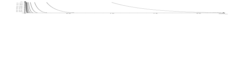
Figure 2: Part of the $(M,n)$ phase diagram for $d=5$ with copies of the non-uniform string branch of Wiseman.

Note that by the Intersection Rule [1] reviewed in Section 2 all the copies in Figure 2 also have the property that the entropy for a solution is less than that of a uniform string of same mass. If we take two copies which both exist for the same mass, we furthermore see from the Intersection Rule that the branch which lies to the left in the $(M,n)$ diagram will have less entropy for a given mass.

We are now capable of addressing an important question regarding Wiseman’s branch (see Figure 5 of [1] for a more detailed plot): Is Wiseman’s branch really starting to have increasing $n$ at a certain point? This question can be addressed using the following rule that we prove below.

• Invertibility Rule
  Consider a curve of solutions in the $(M,n)$ phase diagram. There are no intersections between the curve and its copies, or between any of the copies, if and only if the curve is described by a well-defined function $M=M(n)$ (i.e. if a given $n$ only corresponds to one $M$).

We call this the Invertibility Rule since we normally would describe a branch by a function $n=n(M)$, and then the Invertibility Rule implies such a function is invertible.

For the non-uniform string branch in Figure 1 the Invertibility Rule implies that the small increase in $n$ in the end of the branch can be ruled out if we also assume the Uniqueness Hypothesis [1] (recalled in Section 2) to be valid. To see this note that the latter assumption implies that an intersection of two branches means in particular that the two branches intersect in the same solution and not just in the same point in the $(M,n)$ diagram. Thus, using the Intersection Rule (see Section 2) we cannot have two branches intersecting twice, and if the non-uniform branch was not invertible, then they clearly would intersect twice since they already both intersect the uniform string branch. It then follows that the non-uniform branch must continue to decrease in $n$, and the small increase that one can see must be from inaccuracies in the numerically computed data.

Although it seems reasonable to assume that the above stated conditions hold, it would be interesting to further examine the behavior of the Wiseman branch at the end.

We conclude by proving the Invertibility Rule. On the one hand, it is clearly true that a curve described by a well-defined function $M=M(n)$ will not have intersections between the curve and its copies, or between any of the copies. On the other hand, consider a continuous curve in the $(M,n)$ phase diagram that is not invertible, so that there are two points $(M_{1},n^{\prime})$ and $(M_{2},n^{\prime})$, $M_{1}<M_{2}$. Consider now two copies of the curve according to the transformation (5.2), one with $k=p$ and the other with $k=q$. Then those two copies intersect if $M_{2}/p^{d-3}>M_{1}/q^{d-3}$. Thus, we have intersections if we can find integers $p$ and $q$ so that $M_{2}/M_{1}>p^{d-3}/q^{d-3}>1$. But that is always possible. This completes the proof.

5.3 Consequences for black hole branch

We finally consider the consequence of the transformation (5.2) for black holes on the cylinder, i.e. the branch that starts at $(M,n)=(0,0)$.

We first comment on what, according to (5.1) and (5.2), the physical meaning is of the $k$’th copy for the black hole branch. From (5.1) it is easy to see that the $k$’th copy of a black hole is $k$ black holes on a cylinder put at equal distance from each other. While these solutions clearly exist they are not classically stable. If we take $k=2$, for instance, it is clear that this solution consisting of two black holes is unstable against perturbation of the relative distance between the black holes. The solution will then obviously decay to a single black hole on a cylinder. More generally, $k$ black holes on a cylinder will decay to a fewer number of black holes when perturbed. Thus, all these solutions with $k>1$ are in an unstable equilibrium. At the level of the entropy this implies that we expect that $S_{{\rm BH},k}(M)<S_{{\rm BH},k^{\prime}}(M)$ for $k>k^{\prime}$.

To see this explicitly, note that the thermodynamics for the small black hole branch is given by

$$S_{\rm BH}(M)=c_{1}M^{\frac{d-1}{d-2}}\ ,\ \ c_{1}=4\pi(d-1)^{-\frac{d-1}{d-2}}\left(\frac{16\pi G_{\rm N}}{\Omega_{d-1}}\right)^{\frac{1}{d-2}}\ ,$$ (5.4)

since it is equal to that of a black hole in $d+1$ dimensional Minkowski space. We can then use (5.2) and (5.4) to compute that the entropy function of the $k$’th copy of the small black hole branch is

$$S_{\rm BH,k}(M)=c_{k}M^{\frac{d-1}{d-2}}\ ,\ \ c_{k}=c_{1}k^{-\frac{1}{d-2}}\ .$$ (5.5)

Since then $c_{k}>c_{k^{\prime}}$ for $k<k^{\prime}$, we get that $S_{k}(M)>S_{k^{\prime}}(M)$ for $k<k^{\prime}$, as we required.

Note that it is not excluded that $n=0$ for all of the black hole branch. This would even fit well intuitively with the fact that (4.8) in that case tells us that the black hole behaves like a point-like object since $\delta M=0$ when varying $R_{T}$. On the other hand it also seem reasonable to expect that the complicated shape of the event horizon of the black hole should have the consequence that there should be some corrections to the flat space thermodynamics. Thus, determining whether $n=0$ or $n>0$ amounts to determining which intuition is right: That the behavior of black holes as objects are given by the shape of the singularity or the shape of the event horizon.

Note also that if $n=0$ for the entire black hole branch the Uniqueness Hypothesis [1] which is recalled in Section 2 must be wrong since then we have an infinite number of different solutions with the same $M$ and $n$.

6 Possible scenarios and phase diagrams

6.1 Review of three proposed scenarios

As mentioned in the introduction, Horowitz and Maeda argued in [5] that a classically unstable uniform black string cannot become a black hole in a classical evolution. More precisely they showed that an event horizon cannot have a circle that shrinks to zero size in a finite affine parameter. This led them to conjecture that there exists a new branch of solutions which are non-uniform neutral black strings with entropy greater than that of the uniform black string with equal mass.

The conjecture of Horowitz and Maeda motivated Gubser in [7] to look for a branch of non-uniform black string solutions, connected to the uniform black string solution in the Gregory-Laflamme critical point where $M=M_{GL}$, by using numerical techniques. The numerical data of Gubser were later improved by Wiseman in [8]. As mentioned above, we depicted the non-uniform branch in the $(M,n)$ phase diagram of Figure 1, in the case $d=5$.

However, as noted by [7], the piece of the non-uniform branch found by [7, 8] cannot be the conjectured Horowitz-Maeda non-uniform solutions. Firstly, it was shown in both [7] and [8] that the entropy of a non-uniform black string on the branch is smaller than that of a uniform black string of the same mass. Secondly, all the new solutions in the branch have masses bigger than the Gregory-Laflamme mass $M_{GL}$. Clearly we need non-uniform solutions with masses $M<M_{GL}$ in order to get the conjectured Horowitz-Maeda non-uniform black strings.

In [7] an ingenious proposal was put forward to remedy this situation. The idea was that the branch should continue and at some point have decreasing mass so that we get solutions with $M<M_{GL}$. Moreover, the entropy on the branch should start becoming higher than that of the corresponding uniform black string with equal mass. If true, it means that the classically unstable uniform string decays classically to the classically stable non-uniform string with the same mass via a first order transition. After this, the non-uniform string decays quantum mechanically to a black hole via another first order transition.

Gubser’s scenario obviously does not address the issue of what happens when one increases the mass of a black hole on a cylinder. One possibility is that the black hole branch simply terminates when the mass reaches the critical value when the black horizon reaches all around the cylinder. Clearly then it should be so that the entropy of a black hole just below the critical mass should be less than that of the uniform black string, so that one can have a first order transition from the black hole to a uniform string of the same mass. In the following we refer to this combined scenario as “Scenario I”.

In [10] it was instead suggested that the black hole phase should go directly into a non-uniform string phase which connects to the uniform string phase at $M=\infty$, i.e. $n\rightarrow 1/(d-2)\mbox{ for }M\rightarrow\infty$. Alternatively the branch could instead approach some other limiting value, i.e. $n\rightarrow n_{\star}\mbox{ for }M\rightarrow\infty$. In this type of combined scenario we thus have two non-uniform black string branches, one that connects to the black hole branch and another that connects to the Gregory-Laflamme point $(M,n)=(M_{\rm GL},1/(d-2))$. We refer to this type of scenario as “Scenario II”.

An entirely different scenario was proposed by Kol in [12], where it was conjectured that the non-uniform string branch found in [7, 8] should be continued all the way to the black hole branch. Since this scenario requires for small masses that the non-uniform black string branch changes topology and becomes the black hole branch, it would in any case not be able to account for the conjectured Horowitz-Maeda non-uniform black strings for small masses. Therefore, the unstable uniform string should instead decay classically in infinite “time”, i.e. affine parameter on the horizon, and become arbitrarily near the black hole branch but never reach it classically. We call Kol’s scenario “Scenario III” below.

A final relevant issue is whether the non-uniform branch is classically stable or unstable, which is presently not known. However, since these solutions were found by applying numerical methods that work by perturbing a solution which then relaxes to a new fixed point, it is likely that the Wiseman branch is classically stable. In this connection it is also worth considering the copies of the Wiseman branch discussed in Section 5.2. On the one hand, the fact that for increasing number $k$ the entropy at a given mass decreases, could suggest that the copies are classically unstable. On the other hand, any pair of copied branches has a different mass range, as can be seen in Figure 2. Moreover, contrary to the black hole copies which constitute separate objects, in this case all copies of non-uniform strings have the same topology. As a consequence we view the classical stability of the Wiseman copies as another open problem.

6.2 Phase diagrams for the three scenarios

We can now try to draw how scenarios I-III should look in the $(M,n)$ phase diagram for $d=5$.

When drawing the scenarios in the following we use the $(M,n)$ phase diagram in Figure 1 as the starting point. However, in that diagram (see also appendix C of [1]) we see that the non-uniform branch starts having increasing $n$, just before it ends. We argued in Section 5 that, under reasonable assumptions, the non-uniform branch in fact has to continue decreasing in $n$. The small increase one can see in Figure 1 could thus possibly be due to inaccuracies of the numerics. In the following we have therefore ignored these last few data points and assumed that $n$ keeps decreasing.

It is also important to note that when we construct the $(M,n)$ phase diagrams below we are following the Intersection Rule [1] reviewed in Section 2 which, among other things, has the consequence that one cannot have two branches intersecting twice, at least not when the branches are described by well-defined functions $n=n(M)$.

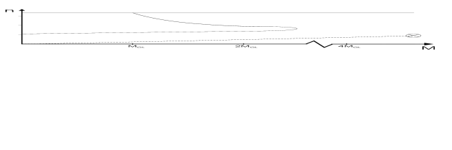
Figure 3: Scenario I. Gubser’s proposal for the non-uniform string branch plus a black hole branch that terminates at the critical point.

In Scenario I that we described above we clearly need to let the non-uniform string branch turn around and reach $M=0$ with $n>0$ since we do not want to cross the black hole branch, and we need $n\geq 0$. We have sketched this scenario in Figure 3. It looks though unlikely that the curve should make such a complicated turn, perhaps one can imagine that the curve has a cusp. This would, however, imply at least a second order phase transition in the point of the cusp which would seem peculiar since the solution does not change phase.

In Figure 3 we have also depicted the black hole phase which in Scenario I terminates at a critical mass when the black hole horizon reaches around the horizon. Note that since we require the entropy at the critical point to be higher than that of a uniform string of the same mass, and since one can integrate up the entropy [1] given a curve in the $(M,n)$ diagram (see eq. (2.6)), we can in fact put bounds on the curve.

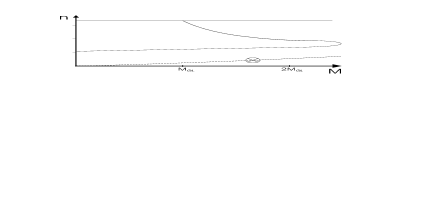
Figure 4: Scenario II. Gubser’s proposal for the non-uniform string branch plus a black hole branch that continues into another non-uniform string branch which continues to arbitrarily large masses.

In Figure 4 we have depicted Scenario II. As described above this scenario again realizes Gubser’s proposal for the non-uniform black string branch that starts at the Gregory-Laflamme point $(M,n)=(M_{\rm GL},1/(d-2))$. But in this scenario the black hole branch continues into another non-uniform string branch that continues for arbitrarily high masses (following the proposal of [10]).

Figure 5: Scenario III. The scenario of Kol where the black hole branch is connected to the non-uniform branch.

In Figure 5 we have depicted Scenario III. This is Kol’s scenario where the non-uniform string branch turns around and meets the black hole branch. A smooth turn again seems problematic, but in this case it seems natural to suppose that there is a cusp precisely at the point where the phase transition between the non-uniform string phase and the black hole phase occurs.

Evidence in support of this scenario was given in Ref. [15], by numerically showing that for sufficient non-uniformity the non-uniform string branch has the property that the local geometry about the minimal horizon sphere approaches the cone metric. They argue furthermore that this implies that the non-uniform branch will not continue beyond the endpoint of Wiseman’s data at $M\simeq 2.3M_{\rm GL}$. If true, this would imply that the other scenarios presented in this section are not viable.

6.3 Other possible scenarios

Each of the three scenarios described above suffers from possible shortcomings. Kol’s scenario in Figure 5 does not have the needed Horowitz-Maeda non-uniform string phase that Horowitz and Maeda argued for in [5]. That can of course possibly turn into a virtue in that the recent paper [6] failed to find an endpoint of the classical decay, suggesting that a stable endpoint in fact does not exists.

On the other hand, the scenarios I and II in Figure 3 and 4 suffer from having a seemingly unnatural U-turn on the curve.

Figure 6: Scenario IV.

One can instead imagine other scenarios which fit with the data in Figure 1. For example one can consider the new scenario depicted in Figure 6. Note that this scenario is constructed so that it has the Horowitz-Maeda non-uniform string branch and so that the above-mentioned U-turn is absent. Note also that the black hole branch is disconnected from the non-uniform string branch originating from the Gregory-Laflamme point $(M,n)=(M_{\rm GL},1/(d-2))$.

Figure 7: Scenario V.

Figure 8: Scenario VI.

Finally, we present the Scenarios V and VI in Figures 7 and 8. These two scenarios both have two non-uniform branches, each of which continues for $M\rightarrow\infty$. Scenario V does not have the conjectured Horowitz-Maeda strings while Scenario VI does.

7 A remarkable near-linear behavior

In this section we report on a remarkable nearly linear behavior of the non-uniform string branch, if one plots $TS$ versus $M$. In Figure 9 we have plotted Wiseman’s data in a $TS$ versus $M$ diagram, and we have fitted a line to the data points in order to demonstrate how near the points falls to a line.

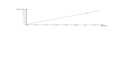
Figure 9: $TS$ versus $M$ plot for the non-uniform string branch. The crosses are the data for Wiseman’s solutions. The line is a linear fit to the data.

Figure 9 shows that the $TS$ versus $M$ data falls very near the line

$$\frac{TS}{T_{\rm GL}S_{\rm GL}}-1=x\left(\frac{M}{M_{\rm GL}}-1\right)\ ,\ \ x=1.12\ .$$ (7.1)

Here $T_{\rm GL}$ and $S_{\rm GL}$ are the temperature and entropy at the Gregory-Laflamme point $(M,n)=(M_{\rm GL},1/(d-2))$. Note that we have chosen the line so that it fits with the first half of the set of data points. Using now Smarr’s formula (2.5) with $d=5$ we see that (7.1) corresponds to the curve

$$n=\frac{8}{3}(x-1)\frac{M_{\rm GL}}{M}+\frac{9-8x}{3}\ ,$$ (7.2)

in the $(M,n)$ diagram. The explicit form of $n(M)$ above, enables us to integrate (2.6) to find the entropy

$$S_{\rm w}=S_{\rm BS}(M_{\rm GL})\left[x\left(\frac{M}{M_{\rm GL}}-1\right)+1\right]^{\frac{3}{2x}}\ ,$$ (7.3)

where the constant of integration is fixed by the intersection point with the uniform string branch. The temperature then also follows easily from Smarr’s formula (2.5).

We have plotted the curve (7.2) along with Wiseman’s data in Figure 10. As one can see, Wiseman’s data deviate more and more from (7.2) as the mass increases. However, it is not clear whether Wiseman’s data is accurate enough to rule out that the exact solutions can fall on a curve of the form (7.2).

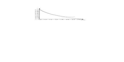
Figure 10: The non-uniform branch of Wiseman [8] (dotted curve) compared to the curve (7.2) (solid curve).

Of course the above observations are of purely phenomenological nature. However, it seems reasonable to expect that there should be some theoretical reasoning leading to the fact that the non-uniform string branch have the linear behavior in Figure 9, at least to a good approximation. This would be interesting to investigate further.

8 Discussion and conclusions

In this paper, we have reported on several new results that enhance the understanding of black holes and strings on cylinders. This development builds partly on the new phase diagram and other tools introduced in Ref. [1].

We presented three main results. Firstly, we proved that the metric of any neutral and static black hole/string solution on a cylinder can be written in the ansatz (3.15), an ansatz that was proposed in [10]. This proof is a generalization of the original proof of Wiseman for $d=5$ in Ref. [13]. The ansatz (3.15) is very simple since it only depends on one function of two variables, which means that most of the gauge freedom of the metric is fixed.

Secondly, we showed that the first law of thermodynamics $\delta M=T\delta S$ holds for any neutral black hole/string on a cylinder. This was proven using the ansatz (3.15) and also the Smarr formula (2.5) of [1]. That any curve of solutions obeys $\delta M=T\delta S$ implies that we do not expect a continuous set of solutions between two given branches in the phase diagram.

The third result is the explicit construction of a solution generator that takes any black/hole string solution and transforms it to a new solution, thus giving a far richer phase diagram. This is a further development of an idea of Horowitz [11] that a black hole/string on a cylinder can be “unwrapped” to give new solutions. We constructed the solution generator using the ansatz (3.15) which furthermore made it possible to write down explicit transformation laws for all the thermodynamic quantities.

Beyond these new results, we have presented a comprehensive analysis of the proposals for the phase structure in light of the new results presented here and in Ref. [1]. In addition to the three previously proposed scenarios, we have listed three new scenarios for the phase structure, all of which could conceivably be true. We have also commented on the viability of the various scenarios.

Finally, we presented a phenomenological observation: Wiseman’s numerical data [8] for the non-uniform string branch lie very near a straight line in a $TS$ versus $M$ diagram. If the true non-uniform branch really lies on a line, that would clearly suggest that only Scenarios IV-VI would have a chance to be true (in principle also Scenario III if the line terminates). Moreover, it would present the tantalizing possibility that perhaps all branches of black holes/strings on cylinders are lines in the $TS$ versus $M$ diagram. That would suggest that the black hole branch lies on the curve given by $n=0$ in the $(M,n)$ phase diagram.

It will be highly interesting to uncover the final and correct $(M,n)$ phase diagram for neutral black holes and strings on cylinders. In the path of finding that, we are bound to learn more about several important questions regarding black holes in General Relativity. We can get a better understanding of the uniqueness properties of black holes, i.e. how many physically different solutions are there for a given $M$ and $n$. We can learn about how “physical” a horizon really is, i.e. does the black hole behave as a point particle, or does it behave as an extended object when put on a cylinder? Finally, we can learn much more about phase transitions in General Relativity. Is Cosmic Censorship upheld or not for a decaying light uniform string? Under which conditions can the topology of an event horizon change? We consider the ideas and results of Ref. [1] and this paper as providing new guiding principles and tools in the quest of understanding the full phase structure of neutral black holes and strings on cylinders so that all these important questions can find their answer.

Appendix A Equivalence of boundary conditions for ansätze in $d=5$

In this appendix, we give a refinement of the original proof [13] that for $d=5$ the three-function conformal ansatz (3.3) of that paper can be mapped onto the two-function ansatz (3.15) proposed in [10].

Our starting point is the conformal ansatz of [13]

$$ds^{2}=-\frac{r^{2}}{m+r^{2}}e^{2A}dt^{2}+e^{2B}(dr^{2}+dz^{2})+e^{2C}(m+r^{2})d\Omega_{3}^{2}\ ,$$ (A.1)

where $A,B,C$ are functions of $(r,z)$, with asymptotic forms

$$A\simeq\frac{a_{2}}{r^{2}}\ ,\ \ B\simeq\frac{b_{2}}{r^{2}}\ ,\ \ C\simeq\frac{c_{1}}{r}+\frac{c_{2}}{r^{2}}\ .$$ (A.2)

The new ingredient of the proof is that we first show that by a suitable change of coordinates the leading term in the boundary condition of the function $C$ can be eliminated, leaving

$$C\simeq\frac{c_{2}+c_{1}^{2}/2}{r^{2}}\ ,$$ (A.3)

while leaving the asymptotic forms of $A$ and $B$ unaffected. The relevance of this step will become clear once we perform the coordinate transformation to the two-function ansatz, as the boundary condition (A.3) will be essential in order to obtain the correct boundary condition for the transformed metric.

To prove this statement we perform the following sequence of coordinate transformations

$$\rho=\sqrt{m+r^{2}}\quad\rightarrow\quad\hat{\rho}=\rho+c\quad\rightarrow\quad\hat{\rho}=\sqrt{m+\hat{r}^{2}}\ .$$ (A.4)

After some algebra the resulting metric in $(\hat{r},z)$ coordinates becomes

$$ds_{6}^{2}=-\frac{\hat{r}^{2}}{m+\hat{r}^{2}}e^{2\hat{A}}dt^{2}+e^{2\hat{B}}[d\hat{r}^{2}+g^{2}(\hat{r})dz^{2}]+e^{2\hat{C}}(m+\hat{r}^{2})d\Omega_{3}^{2}\ ,$$ (A.5)

with asymptotic conditions

$$\hat{A}\simeq\frac{a_{2}}{\hat{r}^{2}}\ ,\ \ \hat{B}\simeq B\simeq\frac{b_{2}}{\hat{r}^{2}}\ ,\ \ \hat{C}\simeq\frac{c_{1}-c}{\hat{r}}+\frac{c_{2}+c_{1}(c_{1}-c)+c^{2}/2}{\hat{r}^{2}}\ ,$$ (A.6)

and

$$g^{2}(\hat{r})\equiv\frac{e^{2B}}{e^{2\hat{B}}}=\frac{(1-\frac{m}{\rho^{2}})}{(1-\frac{m}{\hat{\rho}^{2}})}=\frac{(1-\frac{m}{(\hat{\rho}-c)^{2}})}{(1-\frac{m}{\hat{\rho}^{2}})}=\frac{(1-\frac{m}{(\sqrt{m+\hat{r}^{2}}-c)^{2}})}{(1-\frac{m}{m+\hat{r}^{2}})}\simeq 1-\frac{2mc}{\hat{r}^{3}}\ .$$ (A.7)

As a result we see that for the specific choice $c=c_{1}$ we can transform to a metric where the boundary condition on $\hat{C}$ becomes

$$\hat{C}\simeq\frac{c_{2}+c_{1}^{2}/2}{r^{2}}\ .$$ (A.8)

However, in the process we have lost the conformal form with one single function multiplying the factor $(d\hat{r}^{2}+dz^{2})$.

We therefore first need to transform back to the original conformal form, which we achieve by changing variables $\hat{r}=u(\tilde{r})$ with the function $u$ satisfying the differential equation

$$\partial_{\tilde{r}}u(\tilde{r})=g(u(\tilde{r}))\ .$$ (A.9)

Then we find the form

$$ds^{2}=-\frac{u^{2}(\tilde{r})}{m+u^{2}(\tilde{r})}e^{2\hat{A}(u(\tilde{r}))}dt^{2}+e^{2\hat{B}(u(\tilde{r}))}[d\tilde{r}^{2}+dz^{2}]+e^{2\hat{C}(u(\tilde{r}))}(m+u^{2}(\tilde{r}))d\Omega_{3}^{2}\ .$$ (A.10)

The differential equation (A.9) is pretty hard to solve, but we only need to examine it asymptotically in order to make sure that no $1/\tilde{r}$ terms in the asymptotic conditions are induced. We thus consider its asymptotic form

$$\partial_{\tilde{r}}u(\tilde{r})=1-\frac{mc}{u^{3}(\tilde{r})}\ ,$$ (A.11)

obtained using (A.7). The solution is

$$u(\tilde{r})=\tilde{r}\left(1+\frac{mc}{2\tilde{r}^{3}}+\ldots\right)\ ,$$ (A.12)

and obeys the desired property.

After this sequence of transformations leading to (A.10), we change notation back to the symbols in (A.1) (but now we may drop the $1/r$ term in the asymptotic boundary condition of $C$). What remains is to show that we can change coordinates to the two-function ansatz (3.4). We do not repeat these steps here, as they can be obtained from the general treatment in Section 3.1 by substituting the particular value $d=5$ in equations (3.5)-(3.14). For that value, these general expressions reduce to the steps that are equivalent to those originally performed in [13].

Appendix B A useful identity for static perturbations

In this appendix we derive an identity which holds for static and Ricci-flat perturbations of a static metric. The identity is the starting point in Section 4 for obtaining an important relation on the variation of the mass $\delta M$ which is independent from the generalized Smarr formula (2.5). The derivation and form of this identity follows the corresponding one in [26] (eq. (12.5.42)) where the four-dimensional case was treated.

Consider in a $D$-dimensional space-time two vector fields $v$ and $w$ satisfying $D_{\mu}v^{\mu}=0$ and $D_{\mu}w^{\mu}=0$. Let $v$ and $w$ be commuting, i.e. $\mathcal{L}_{v}w=\mathcal{L}_{w}v=0$. It is not difficult to show that as a consequence one has $D_{\mu}v^{[\mu}w^{\nu]}=0$ where $2v^{[\mu}w^{\nu]}=v^{\mu}w^{\nu}-v^{\nu}w^{\mu}$. Using Gauss theorem we then get that

$$\int_{S_{1}}dS_{\mu\nu}v^{[\mu}w^{\nu]}=\int_{S_{2}}dS_{\mu\nu}v^{[\mu}w^{\nu]}\ .$$ (B.1)

We now consider a static metric $g_{\mu\nu}$ and take $w$ as the vector field $w=\frac{\partial}{\partial t}$ and let $v$ be given so that $\frac{\partial}{\partial t}v^{\mu}=0$. First we see that $D_{\mu}w^{\mu}=0$ since $\Gamma^{\mu}_{\mu 0}=0$ because $g_{\mu\nu}$ is static with respect to $t=x^{0}$. Secondly we see that $(\mathcal{L}_{w}v)^{\mu}=\partial_{0}v^{\mu}-v^{\alpha}\partial_{\alpha}w^{\mu}=0$ so $[v,w]=0$. Thus, we only need to require that $\partial_{0}v^{\mu}=0$ and $D_{\mu}v^{\mu}=0$ to get the desired properties of $v$ and $w$

Consider now a static perturbation of the metric $\delta g_{\mu\nu}$ which leaves the Ricci tensor unchanged, i.e. $\delta R_{\mu\nu}=0$. Using the Palatini identity $\delta R_{\mu\nu}=D_{\nu}\delta\Gamma^{\alpha}_{\mu\alpha}-D_{\alpha}\delta\Gamma^{\alpha}_{\mu\nu}$ we can write $g^{\mu\nu}\delta R_{\mu\nu}$ as

$$g^{\mu\nu}\delta R_{\mu\nu}=-D_{\mu}v^{\mu}\ ,\ \ v^{\mu}=D_{\nu}\left[g^{\mu\alpha}g^{\nu\beta}\delta g_{\alpha\beta}-g^{\mu\nu}g^{\alpha\beta}\delta g_{\alpha\beta}\right]\ .$$ (B.2)

Using now the requirement $\delta R_{\mu\nu}=0$ as well as that $\delta g_{\mu\nu}$ is a static perturbation, we find that the $v$ defined in (B.2) satisfies $\partial_{0}v^{\mu}=0$ and $D_{\mu}v^{\mu}=0$ as desired.

We are now ready to state the advertised identity which generalizes Wald’s identity (12.5.42) in [26]. Consider a static metric $g_{\mu\nu}$ and a static perturbation of the metric $\delta g_{\mu\nu}$ with $\delta R_{\mu\nu}=0$. Choose two oppositely oriented disjoint $(D-2)$-dimensional surfaces $S_{1}$ and $S_{2}$ so that $\partial V=S_{1}\cup S_{2}$ for some $(D-1)$ dimensional volume $V$. Then we have that

$$\int_{S_{1}}dS_{\mu\nu}v^{\mu}w^{\nu}=\int_{S_{2}}dS_{\mu\nu}v^{\mu}w^{\nu}\ ,$$ (B.3)

with

$$v^{\mu}=D_{\nu}\left[g^{\mu\alpha}g^{\nu\beta}\delta g_{\alpha\beta}-g^{\mu\nu}g^{\alpha\beta}\delta g_{\alpha\beta}\right]\ ,\ \ w=\frac{\partial}{\partial t}\ .$$ (B.4)

References

- [1] T. Harmark and N. A. Obers, “New phase diagram for black holes and strings on cylinders,” hep-th/0309116. To appear in Class. Quant. Grav..
- [2] B. Kol, E. Sorkin, and T. Piran, “Caged black holes: Black holes in compactified spacetimes I – theory,” hep-th/0309190.
- [3] R. Gregory and R. Laflamme, “Black strings and p-branes are unstable,” Phys. Rev. Lett. 70 (1993) 2837–2840, hep-th/9301052.
- [4] R. Gregory and R. Laflamme, “The instability of charged black strings and p-branes,” Nucl. Phys. B428 (1994) 399–434, hep-th/9404071.
- [5] G. T. Horowitz and K. Maeda, “Fate of the black string instability,” Phys. Rev. Lett. 87 (2001) 131301, hep-th/0105111.
- [6] M. W. Choptuik et al., “Towards the final fate of an unstable black string,” Phys. Rev. D68 (2003) 044001, gr-qc/0304085.
- [7] S. S. Gubser, “On non-uniform black branes,” Class. Quant. Grav. 19 (2002) 4825–4844, hep-th/0110193.
- [8] T. Wiseman, “Static axisymmetric vacuum solutions and non-uniform black strings,” Class. Quant. Grav. 20 (2003) 1137–1176, hep-th/0209051.
- [9] R. Gregory and R. Laflamme, “Hypercylindrical black holes,” Phys. Rev. D37 (1988) 305.
- [10] T. Harmark and N. A. Obers, “Black holes on cylinders,” JHEP 05 (2002) 032, hep-th/0204047.
- [11] G. T. Horowitz, “Playing with black strings,” hep-th/0205069.
- [12] B. Kol, “Topology change in general relativity and the black-hole black-string transition,” hep-th/0206220.
- [13] T. Wiseman, “From black strings to black holes,” Class. Quant. Grav. 20 (2003) 1177–1186, hep-th/0211028.
- [14] T. Harmark and N. A. Obers, “Black holes and black strings on cylinders,” Fortsch. Phys. 51 (2003) 793–798, hep-th/0301020.
- [15] B. Kol and T. Wiseman, “Evidence that highly non-uniform black strings have a conical waist,” Class. Quant. Grav. 20 (2003) 3493–3504, hep-th/0304070.
- [16] R. Casadio and B. Harms, “Black hole evaporation and large extra dimensions,” Phys. Lett. B487 (2000) 209–214, hep-th/0004004.
- [17] R. Casadio and B. Harms, “Black hole evaporation and compact extra dimensions,” Phys. Rev. D64 (2001) 024016, hep-th/0101154.
- [18] G. T. Horowitz and K. Maeda, “Inhomogeneous near-extremal black branes,” Phys. Rev. D65 (2002) 104028, hep-th/0201241.
- [19] P.-J. De Smet, “Black holes on cylinders are not algebraically special,” Class. Quant. Grav. 19 (2002) 4877–4896, hep-th/0206106.
- [20] B. Kol, “Speculative generalization of black hole uniqueness to higher dimensions,” hep-th/0208056.
- [21] E. Sorkin and T. Piran, “Initial data for black holes and black strings in 5d,” Phys. Rev. Lett. 90 (2003) 171301, hep-th/0211210.
- [22] A. V. Frolov and V. P. Frolov, “Black holes in a compactified spacetime,” Phys. Rev. D67 (2003) 124025, hep-th/0302085.
- [23] R. Emparan and R. C. Myers, “Instability of ultra-spinning black holes,” JHEP 09 (2003) 025, hep-th/0308056.
- [24] J. Traschen and D. Fox, “Tension perturbations of black brane spacetimes,” gr-qc/0103106.
- [25] P. K. Townsend and M. Zamaklar, “The first law of black brane mechanics,” Class. Quant. Grav. 18 (2001) 5269–5286, hep-th/0107228.
- [26] R. M. Wald, General Relativity. The University of Chicago Press, 1984.