The Non-Commutative $\lambda\phi^{4}$ Model

Abstract

In the recent years, field theory on non-commutative (NC) spaces has attracted a lot of attention. Most literature on this subject deals with perturbation theory, although the latter runs into grave problems beyond one loop. Here we present results from a fully non-perturbative approach. In particular, we performed numerical simulations of the $\lambda\phi^{4}$ model with two NC spatial coordinates, and a commutative Euclidean time. This theory is lattice discretized and then mapped onto a matrix model. The simulation results reveal a phase diagram with various types of ordered phases. We discuss the suitable order parameters, as well as the spatial and temporal correlators. The dispersion relation clearly shows a trend towards the expected IR singularity. Its parameterization provides the tool to extract the continuum limit.

11.10.Nx, 11.30.Cp, 05.50.+q

Preprint HU-EP-03/69

1 Field Theory on a Non-Commutative Space

The simplest way to introduce non-commutative (NC) coordinates is to impose the relation

$$[\hat{x}_{\mu},\hat{x}_{\nu}]=i\Theta_{\mu\nu}\ ,$$ (1)

$\Theta$ being a constant, anti-symmetric tensor, while $\hat{x}_{\mu}$ are Hermitian coordinate operators (which cannot be diagonalized simultaneously). This relation leads to an uncertainty in c-space, $\Delta x_{\mu}\Delta x_{\nu}>0$ $(\mu\neq\nu)$. The pre-history of this idea involves private communication among celebrities like Heisenberg, Peierls, Pauli and Oppenheimer. The latter asked his student Snyder to work it out, which yielded the first publication about physics on a NC space [1], followed immediately by Ref. [2].

The mathematical framework for the formulation of field theory on NC spaces was worked out in the eighties [3]. However, a real boom of interest was triggered only in the late nineties by the observation that string and M theory at low energy in a magnetic background field can be identified with NC field theory [4]. This boom persists up to now, as is manifest from new preprints on this subjects appearing day after day.

The identification of Refs. [5, 4] transforms the background field into a $\Theta$ term. The same idea has been around in solid state physics long before, where it led to a new description of the quantum Hall effect [6]. The origin of this idea goes back to Peierls: an electron in a strong magnetic background field has an obvious description by NC coordinates, where the magnetic field is replaced by non-commutativity, with an extent inverse to the magnetic field strength.

To illustrate this fundamental property in the simplest possible way, we consider an electron moving in a plane, with position $\vec{x}=(x_{1},x_{2},0)$, exposed to a magnetic field $\vec{B}=(0,0,B)$. If this field is strong, the Lagrangian

$$L[\vec{x},\dot{\vec{x}}]=\frac{m}{2}\dot{\vec{x}}^{\,2}+eB\epsilon_{ij}x_{i}\dot{x}_{j}\ ,\qquad(i,j=1,2)$$ (2)

can be reduced to the second term, so that the canonical momentum reads

$$\Pi_{j}=\frac{\partial L}{\partial\dot{x}_{j}}=eB\epsilon_{ij}x_{i}\ .$$ (3)

Applying now the canonical quantization rule

$$[\hat{x}_{i},\hat{\Pi}_{j}]=i\hbar\delta_{ij}$$ (4)

we arrive at

$$[\hat{x}_{i},\hat{\Pi}_{i}]=eB\epsilon_{ij}[\hat{x}_{i},\hat{x}_{j}]\ .$$ (5)

Indeed, together with eq. (3) this corresponds to the NC relation

$$[\hat{x}_{i},\hat{x}_{j}]=i\Theta_{ij}\ ,\qquad\Theta_{ij}=\frac{\hbar}{e}\frac{1}{B}\epsilon_{ij}:=\theta\epsilon_{ij}\ .$$ (6)

This illustration of Peierls’ map, along with a more precise derivation based on the Hamiltonian formalism, is explained for instance in Ref. [7].

Hence one motivation to study NC field theory is simply its application as a formalism to describe certain effects in the commutative world. Such effects are typically related to a background field, which is then transformed away by going non-commutative.

However, in addition to that concept, the present fashion also includes studying the possibility of a really NC space-time. A deep, qualitative difference from the commutative space-time is the occurrence of a non-locality of range $\sqrt{\|\Theta\|}$. Obviously this feature raises conceptual problems, but from the optimistic point of view it is a source of hope for a link to quantum gravity.

In fact, there is a claim that attempts to merge quantum theory and gravitation imply quite generally a NC space. To illustrate this line of thought, we quote a simple Gedankenexperiment.

Some event is measured with accuracy $\Delta x$, $\Delta y$, $\Delta z$, $\Delta t$. This requires an energy concentration, which implies a gravitational field. In the extreme case, the latter imposes an event horizon beyond the uncertainty, so that the event is effectively invisible. One may now evaluate the condition for avoiding this, i.e. for dealing with actually detectable events. On the Planck scale, an estimate in Ref. [8] suggests the constraints

$$\Delta x\Delta y+\Delta x\Delta z+\Delta y\Delta z\geq 1\ ,$$

$$(\Delta x+\Delta y+\Delta z)\Delta t\geq 1\ ,$$ (7)

so that the NC space seems indeed natural as soon as gravity is involved.

However, this argument should come along with at least one remark of caution: much of the literature excludes time from the non-commutativity, including the remainder of this article. Otherwise the problems related to causality [9] are especially severe. From the above argument, however, this step would not be justified.

The last point is also related to the question if and how the Wick rotation from an Euclidean to a Minkowski signature can be performed in the NC world. This is not ultimately settled yet, but in our case of a commutative time the issue is less problematic. Anyhow, here we work in Euclidean space, and we are happy there, without worrying about the details of the transition to the NC Minkowski space.

Since the idea that our space could really be NC is fashionable, of course there are already numerous speculations about possible measurements of $\Theta$.

One suggestion is based on the deformation of the photon dispersion relation due to $\Theta$ [10]. Blazers (highly active galactic nuclei) emit bursts of photons over a broad energy spectrum. Assuming this emission to be simultaneous, a relative delay could in principle establish bounds on $\Theta$. However, in addition to experimental difficulties, the knowledge about the deformed dispersion is also limited to a one loop calculation [11].

The last limitation is especially worrisome in the light of the fact that most higher loop calculations are not feasible yet — no systematic machine is known for them. Perturbation theory is even more complicated than in the good old commutative space, which is in striking contradiction to the original hope that $\Theta$ would simplify the perturbative renormalization [1]. It is true that part of the UV singularities are removed due to the non-commutativity, but others remain, in particular those in the planar diagrams [12]. What makes the situation worse is that the non-planar divergences do not just disappear, but they are rather turned into IR singularities with respect to external momenta. This effect is denoted as UV/IR mixing [13]. At this point we want to give again just a simple intuitive reason; we will be somewhat more explicit below in the framework of the $\lambda\phi^{4}$ model.

We return to simple natural units $\hbar=1$, without involving the Planck scale any more. If we combine Heisenberg’s uncertainty $\Delta x_{j}\sim 1/\Delta p_{j}$ with the NC relation

$$\Delta x_{j}\sim\Theta_{ij}/\Delta x_{i}\sim\Theta_{ij}\Delta p_{i}\ ,\qquad(i\neq j)$$ (8)

we see that for $\Delta p_{j}\to 0$ the other momentum components explode, $\Delta p_{i}\to\infty$, and vice versa. This also suggests that in addition to the Heisenberg term, $\Delta x_{j}$ picks up a term linear in the $\Delta p_{i}$, which may be denoted as a “string modification” of the uncertainty principle.

In the work to be presented here we are going to consider a 3d Euclidean space with a commutative Euclidean time $t$ and two NC spatial coordinates, which obey

$$[\hat{x}_{\mu},\hat{x}_{\nu}]=i\theta\epsilon_{\mu\nu}\ .$$ (9)

We are happy to avoid the horror of NC perturbation theory by taking the fully non-perturbative approach of numerical simulations. To this end, the space should first be lattice discretized, as in the commutative world. Here we also need a second step, namely a mapping of the lattice field theory onto a matrix model, which will be described in Section 2. At this point we only comment on the general structure of a 2d NC lattice of spacing $a$, following Ref. [14].

The restriction of the spectrum of $\hat{x}_{\mu}$ to the lattice sites corresponds to the operator identity

$$\exp\Big{(}i\frac{2\pi}{a}\hat{x}_{\mu}\Big{)}=\hat{1}\!\!1\ .$$ (10)

As in the commutative case, we want the momentum components $k_{\mu}$ to be periodic over the Brillouin zone,

$$\exp\left(i\Big{[}k_{\mu}+\frac{2\pi}{a}\Big{]}\hat{x}_{\mu}\right)=\exp(ik_{\mu}\hat{x}_{\mu})\ .$$ (11)

Multiplying both sides by the factor $\exp(-ik_{\nu}\hat{x}_{\nu})$ now leads to consistency with eq. (10), iff

$$\frac{\theta}{2a}k_{\mu}\in\mathbb{Z}\ ,$$ (12)

which has amazing consequences: any NC lattice is automatically periodic, say over a lattice volume $L\times L$. Then the discrete momenta $k^{(n)}=\frac{2\pi}{aL}n$ occur, where $n_{\mu}\in\mathbb{Z}$. The non-commutativity parameter can be identified as

$$\theta=\frac{1}{\pi}a^{2}L\ .$$ (13)

We see that the continuum limit $a\to 0$ and the thermodynamic limit $L\to\infty$ are manifestly entangled, which is again an aspect of UV/IR mixing. Taking these two limits simultaneously in such a way that $\theta$ remains constant is denoted as the double scaling limit.

2 The non-commutative $\lambda\phi^{4}$ model

NC field theories can be formulated in a form which looks similar to the commutative world, if all the fields are multiplied by the star product (or Moyal product),

$$f(x)\star g(x):=\exp\left(\frac{1}{2}i\Theta_{\mu\nu}\frac{\partial}{\partial x_{\mu}}\frac{\partial}{\partial y_{\nu}}\right)f(x)\,g(y)|_{x=y}\ .$$ (14)

In the particular case of bilinear terms in an action, the star product is equivalent to the ordinary product, hence in these terms the star product is not needed.

Based on these rules, we can write down for instance the action of the NC $\lambda\phi^{4}$ model,

$$S[\phi]=\int d^{d}x\,\Big{[}\frac{1}{2}\partial_{\mu}\phi\,\partial_{\mu}\phi+\frac{m^{2}}{2}\phi^{2}+\frac{\lambda}{4}\phi\star\phi\star\phi\star\phi\Big{]}\ .$$ (15)

Since only the self-interaction term involves $\Theta$, the coupling strength $\lambda$ also determines the extent of NC effects in this model.

To render the above star product rules plausible, we consider the composition of plane wave operators,

$$e^{ip_{\mu}\hat{x}_{\mu}}\cdot e^{iq_{\nu}\hat{x}_{\nu}}=\exp\Big{(}-\frac{i}{2}p_{\mu}\Theta_{\mu\nu}q_{\nu}\Big{)}\,e^{i(p+q)_{\mu}\hat{x}_{\mu}}\ .$$ (16)

This provides a prescription for the translation from the commutative product $e^{ipx}e^{iqx}$ into a NC formulation in terms of $x$, i.e. without using the operator $\hat{x}$,

$$e^{ipx}e^{iqx}\to e^{-\frac{i}{2}p_{\mu}\Theta_{\mu\nu}q_{\nu}}e^{i(p+q)x}:=e^{ipx}\star e^{iqx}\ .$$ (17)

More generally, we can adopt this translation rule to the product of fields, which can be decomposed into plane waves,

$$\phi(x)\psi(x)\to\phi(x)\,e^{\frac{i}{2}\overset{\leftarrow}{{\partial_{\mu}}}\Theta_{\mu\nu}\overset{\to}{{\partial_{\nu}}}}\,\psi(x):=\phi(x)\star\psi(x)\ .$$ (18)

Turning now to the peculiarity of bilinear terms, it is easy to see that in

$$\int d^{d}x\,\phi(x)\star\psi(x)=\int d^{d}x\,\phi(x)\Big{[}1-\frac{i}{2}\overset{\leftarrow}{{\partial_{\mu}}}\Theta_{\mu\nu}\overset{\to}{{\partial_{\nu}}}+\dots\Big{]}\psi(x)\overset{!}{=}\int d^{d}x\,\phi(x)\psi(x)$$

all the terms in the square bracket which involve $\Theta$ cannot contribute, based on partial integration and $\Theta_{\mu\nu}=-\Theta_{\nu\mu}$.

The one loop level of this model is suitable for the illustration of the general properties of NC perturbation theory that we mentioned in Section 1.

To this end, we consider the one loop level of the one particle irreducible 2-point function to the action (15), i.e. the $n=1$ contribution to

$$\langle\phi(p)\phi(-p)\rangle=\sum_{n=0}^{\infty}\lambda^{n}\Gamma^{(n)}(p)\ .$$ (19)

It contains a planar and a non-planar term,

$$\Gamma_{planar}^{(1)}=\frac{1}{3}\int\frac{d^{d}k}{(2\pi)^{d}}\frac{1}{k^{2}+m^{2}}\ ,\quad\Gamma_{non-planar}^{(1)}=\frac{1}{6}\int\frac{d^{d}k}{(2\pi)^{d}}\frac{\exp(ik_{\mu}\Theta_{\mu\nu}p_{\nu})}{k^{2}+m^{2}}\ ,$$ (20)

which are illustrated in Fig. 1.

Figure 1: The planar and non-planar one loop contribution to the two–point function (19), given in eqs. (20).

We see that the planar part is independent of $\Theta$ [12], whereas the non-planar part is affected by UV/IR mixing [13]. To reveal what this means, we introduce a momentum cut-off $\Lambda$ and obtain [14] ( for $m>0$)

$$\Gamma_{non-planar}^{(1)}(p)=\frac{m^{(d-2)/2}}{6\,(2\pi)^{d/2}}\Big{(}\frac{4}{\Lambda^{2}}-p_{\mu}\Theta^{2}_{\mu\nu}p_{\nu}\Big{)}^{(2-d)/4}K_{\frac{d-2}{2}}\Big{(}m\sqrt{\frac{4}{\Lambda^{2}}-p_{\mu}\Theta^{2}_{\mu\nu}p_{\nu}}\Big{)}\ ,$$

where $\Theta^{2}_{\mu\nu}=\Theta_{\mu\rho}\Theta_{\rho\nu}$ and $K$ is the modified Bessel function. In particular in $d=4$ the divergent part is given by

$$\Gamma_{non-planar}^{(1)}(p) = \frac{1}{96\pi^{2}}\left(\Lambda_{\rm eff}^{2}-m^{2}\ln\Big{(}\frac{\Lambda_{\rm eff}^{2}}{m^{2}}\Big{)}\right)+{\rm finite~{}terms}\ ,$$

$$\Lambda_{\rm eff}^{2} = \frac{1}{\frac{1}{\Lambda^{2}}-p_{\mu}\Theta^{2}_{\mu\nu}p_{\nu}}\ .$$ (21)

In general the effective cut-off $\Lambda_{\rm eff}$ remains finite in the UV limit $\Lambda\to\infty$, but it diverges if we take simultaneously the IR limit $p\to 0$.

A comprehensive one loop study of the NC $\lambda\phi^{4}$ model in various dimensions has been performed in Ref. [15]. That work dealt with a self-consistent Hartree-Fock type approximation, which would be exact for the $O(N)$ model at large $N$. The authors assumed its validity also for the $N=1$ theory and conjectured in particular a prediction for the phase diagram. As a general feature, the system undergoes some ordering at $m^{2}\ll 0$, which corresponds in some sense to a very low temperature. If $m^{2}$ is lowered to that point, Gubser and Sondhi predict in $d=3$ and $d=4$ the following behavior:

• At small $\theta$, there is an Ising transition to a uniform order, as in the commutative case.

• At larger $\theta$, the ordered state has a structure of stripes or even more complicated patterns.

Note that the formation of such a stripe order implies the spontaneous breaking of translation invariance. Therefore Gubser and Sondhi did not expect this phase in $d=2$. We will return to this point at the end of Section 3.

The same question was also studied by means of a renormalization group analysis [16].

Our goal was a non-perturbative, quantitative verification of that qualitative conjecture, and our methods are Monte Carlo simulations. The lattice formulation (c.f. Section 1) is not hard to write down, but it is very hard to simulate due to the star product. The way out which enabled efficient simulations is a mapping onto a dimensionally reduced matrix model, as suggested in Ref. [17]. This method is a refinement of the matrix model approach to NC gauge theory in the continuum [18].

Assume the field $\phi(\vec{x},t)$ to be defined on a $N^{2}\times T$ lattice of unit spacing. According to Ref. [17] the following action is equivalent to the lattice action:

$$S[\bar{\phi}] = N\,{\rm Tr}\sum_{t=1}^{T}\Big{[}\frac{1}{2}\sum_{\mu=1}^{2}\Big{(}\Gamma_{\mu}\bar{\phi}(t)\Gamma_{\mu}^{\dagger}-\bar{\phi}(t)\Big{)}^{2}$$ (22)

$$+\frac{1}{2}\Big{(}\bar{\phi}(t+1)-\bar{\phi}(t)\Big{)}^{2}+\frac{m^{2}}{2}\bar{\phi}^{2}(t)+\frac{\lambda}{4}\bar{\phi}^{4}(t)\Big{]}\ .$$

Here $\bar{\phi}(t)$ ($t=1\dots T$) are Hermitian $N\times N$ matrices. In the (commutative) time direction the kinetic term takes the ordinary discrete form. The quartic term — which is in the original formulation plagued by repeated star products — looks relatively simple now, although it should be noted that these matrices are not sparse (in contrast to typical lattice formulations of commutative field theory), hence the fourth power requires some computation. However, much of the complication due to the NC geometry is now manifest in the non-standard kinetic term in the spatial directions. The so-called twist eaters $\Gamma_{\mu}$ provide the shift which corresponds to one lattice unit, if they obey the ’t Hooft algebra

$$\Gamma_{\mu}\Gamma_{\nu}={\cal Z}_{\nu\mu}\Gamma_{\nu}\Gamma_{\mu}\ .$$ (23)

The tensor ${\cal Z}_{\mu\nu}={\cal Z}_{\nu\mu}^{*}$ is called the twist factor. In general it may have the form ${\cal Z}_{12}=e^{2\pi ik/N}$, where $k\in\mathbb{Z}$. The representation of the twist eaters that we choose [20, 21] requires the twist to have the specific form

$${\cal Z}_{12}=\exp\Big{(}i\frac{N+1}{N}\pi\Big{)}\ ,$$ (24)

as we are going to sketch below. Comparison with the general form shows that then $N$ has to be odd. The lattice model and the matrix model are connected by Morita equivalence, which means that their algebras are fully identical.

Let us go back to the NC lattice formulation discussed in Section 1. Since the momenta are discrete, we should not use the (unbounded) operators $\hat{x}_{\mu}$, $\mu=1,2$ to describe the lattice sites. Instead we introduce the unitary operators $\hat{Z}_{\mu}=\exp(\frac{2\pi}{La}i\hat{x}_{\mu})$, which obey the commutation relation

$$\hat{Z}_{\mu}\hat{Z}_{\nu}=\exp\Big{(}-\frac{4\pi^{2}}{a^{2}L^{2}}i\Theta_{\mu\nu}\Big{)}\hat{Z}_{\nu}\hat{Z}_{\mu}=\exp\Big{(}-\frac{4\pi}{L}i\epsilon_{\mu\nu}\Big{)}\hat{Z}_{\nu}\hat{Z}_{\mu}\ ,$$ (25)

where we used $\Theta_{\mu\nu}=\theta\epsilon_{\mu\nu}$ and eq. (13). The lattice translation operator $\hat{D}_{\mu}=\exp(a\hat{\partial}_{\mu})$ is supposed to fulfill the relation

$$\hat{D}_{\mu}\hat{Z}_{\nu}\hat{D}_{\mu}^{\dagger}=e^{2\pi ai\delta_{\mu\nu}/L}\hat{Z}_{\nu}\ .$$ (26)

The issue is now to find a matrix solution for the conditions (25) and (26). This solution is unique only up to symmetry transformations, hence one may end up with different twist factors. We assumed the unitary twist eaters to take the form

$$\Gamma_{1}=\left(\begin{array}[]{cccccc}0&1&0&.&.&.\\ 0&.&1&.&.&.\\ .&.&.&1&.&.\\ .&.&.&.&.&.\\ .&.&.&.&.&1\\ 1&.&.&.&.&0\end{array}\right)\quad,\quad\Gamma_{2}=\left(\begin{array}[]{cccccc}1&0&.&.&.&~{}.\\ 0&{\cal Z}_{21}&0&.&.&~{}.\\ 0&0&{\cal Z}_{21}^{2}&.&.&~{}.\\ .&.&.&{\cal Z}_{21}^{3}&.&~{}.\\ .&.&.&.&.&~{}.\\ 0&.&.&.&.&~{}.\end{array}\right)$$

where ${\cal Z}_{12}={\cal Z}_{21}^{*}$ characterizes the twist. This ansatz solves indeed the conditions (25) and (26), iff we choose the twist of eq. (24) [21]. However, a different ansatz for $\hat{D}_{\mu}$ resp. $\hat{Z}_{\mu}$ may lead to an alternative solution with a modified twist, see e.g. Ref. [22].

3 Numerical results

An overview of our numerical results is given by the phase diagram in Fig. 2. For a suitable re-scaling of the axis, this diagram stabilizes with increasing $N=T$. At strongly negative $m^{2}$ (corresponding to a very low temperature) the system seeks some order. At small self-interaction $\lambda$ the non-commutativity is not much amplified and the systems behaves as in the commutative world, i.e. it is ordered uniformly. At larger $\lambda$ a new striped phase sets in, in the spirit of Ref. [15]. Such a phase is not known in the commutative $\lambda\phi^{4}$ model, but similar phenomena appear in solid state physics, see for instance Ref. [23]. In that phase, a non-zero mode condenses, so that the ground states correspond to a stripe pattern, or to more complicated checker-field-type patterns. Typical examples for the various cases are shown in Fig. 3.

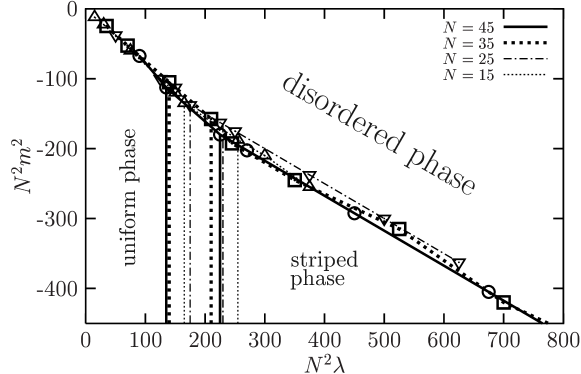
Figure 2: The phase diagram of the NC $\lambda\phi^{4}$ model, explored by means of numerical simulations. Since it contains a new type of phase we conclude: this diagram of phases simply amazes.

(a) $N=45,~{}\lambda=0.044,~{}m^{2}=-0.011$

(b) $N=45,~{}\lambda=0.044,~{}m^{2}=-0.11$

(c) $N=45,~{}\lambda=0.22,~{}m^{2}=-0.2$

(d) $N=35,~{}\lambda=10,~{}m^{2}=-4$

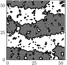
(e) $N=55,~{}\lambda=50,~{}m^{2}=-22$

Figure 3: Snapshots of typical, well thermalized configurations in different sectors of the phase diagram: disordered and uniformly ordered (above), and patterns of two stripes parallel to an axis, two diagonal stripes and finally four stripes (below). The dark and bright areas correspond to $\phi>0$, $\phi<0$.

The transition from disorder to order can be localized well and it appears to be second order. On the other hand, the transition between the uniform and the striped phase is more difficult to localize and it is expected to be of first order.

The order parameter that was used here is based on the spatial Fourier transform of the scalar field, $\tilde{\phi}(\vec{p},t)$. We average over the time direction and turn it such that an eventually condensated mode can be detected optimally. This is done be introducing the function

$$M(k)=\frac{1}{NT}\ ^{\rm max}_{k=|\vec{p}|N/2\pi}\,\left|\sum_{t=1}^{T}\tilde{\phi}(\vec{p},t)\right|\ ,$$ (27)

and its expectation value is our order parameter, sensitive to the mode $k$. In particular, $\langle M(0)\rangle$ is the standard order parameter for the $Z_{2}$ symmetry, $\langle M(1)\rangle$ is the staggered order parameter that detects patterns of two stripes parallel to one of the axes as in Fig. 3 below on the left, $\langle M(\sqrt{2})\rangle$ detects a diagonal two-stripe pattern as in Fig. 3 below in the center, $\langle M(2)\rangle$ detects a pattern of four stripes parallel to one of the axes as in Fig. 3 below on the right, etc. We also measured the connected two-point functions of $M(k)$, the peak of which allowed us to localize the order–disorder phase transition in the diagram of Fig. 2 to a high precision.

Next we consider the spatial correlator at a fixed time,

$$C(\vec{x})=\langle\phi(\vec{0},t)\phi(\vec{x},t)\rangle\ .$$ (28)

As it can be expected, in the disordered phase this decay is fast, but in contrast to our daily experience in the commutative world, it is in general not exponential (nor polynomial), as Fig. 4 (on the left) shows. It may be plausible that the spatial decay behavior is somehow distorted by the NC geometry; what is perhaps more surprising is that the decay moves closer to an exponential as $\lambda$ increases (so that the NC effects are expected to be enhanced), see Fig. 4 (on the right). This observation might be explained in the light of the pole structure described in Ref. [13].

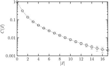
(a) $\lambda=0.06,~{}m^{2}=-0.015$

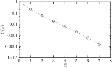
(b) $\lambda=2,~{}m^{2}=-0.3$

Figure 4: Decay of the spatial correlator $C(\vec{x})$ defined in eq. (28) at $N=35$ in the disordered phase, close to the ordering phase transition. On the left we see a clear deviation from the exponential decay. At larger $\lambda$ (on the right) the standard exponential behavior is approximated.

Turning now to the striped phase, the pattern with stripes parallel to one of the axes can be visualized well by plotting $C(x_{1},0)$ and $C(0,x_{2})$. In Fig. 5 we show two examples where the cuts through a configuration of two stripes parallel to an axis (on the left) resp. two diagonal stripes (on the right) can easily be recognized.

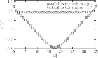
(a) $\lambda=0.6,~{}m^{2}=-0.7$

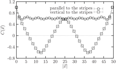
(b) $\lambda=6,~{}m^{2}=-4$

Figure 5: The profile of $C(x_{1},0)$ and $C(0,x_{2})$ at $N=35$ for two stripes parallel to an axis (left) and two diagonal stripes, as they occur at stronger coupling (right).

Now we want to consider the correlations in the direction of the Euclidean time. More precisely, we consider the correlators of two fields $\tilde{\phi}(\vec{p},t)$ at the same momentum $\vec{p}$ but at different times. For instance, Fig. 6 on the left shows

$$G(\tau):=\langle\tilde{\phi}(\vec{p}=\vec{0},t)\tilde{\phi}(\vec{p}=\vec{0},t+\tau)\rangle$$ (29)

in the disordered phase, close to the phase transition. Since the time direction is commutative, we rather expect here the usual behavior, and indeed these correlators follow neatly the exponential with periodic boundary conditions, i.e. a cosh shape. This shape allows us to extract the energy at rest — or effective mass — in the exponentially dominated sector (not too close to the center) as

$$E(\vec{p}=\vec{0})=-\ln\frac{G(\tau+1)}{G(\tau)}\ .$$ (30)

By varying $\tau$ we find a convincing plateau, see Fig. 6 on the right.

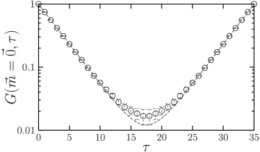
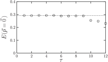
Figure 6: On the left: the temporal correlator $G(\tau)$, defined in eq. (29), at $N=35$, $\lambda=0.29$, $m^{2}=-0.11$. On the right we show the rest energy extracted at different values of $\tau$ according to eq. (30), which has a clear plateau.

We can now repeat this procedure also at non-vanishing momenta $\vec{p}$, which finally yields the full dispersion relation $E(\vec{p})$. We still stay in the disordered phase, close to the ordering transition. If we are close to the uniform order (small $\lambda$), the dispersion has its usual linear shape (up to finite size corrections) as in the commutative case, see Fig. 7 on the left. However, the shape changes if we move to the vicinity of the striped phase, see Fig. 7 on the right. Now the rest energy increases, since the effects of UV/IR mixing set in. In the large $N$ double scaling limit it is expected to diverge. The minimum moves to a finite value of the momentum, which corresponds to the stripe patterns shown in Fig. 3.

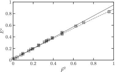
(a) $N=45,~{}\lambda=0.035,~{}m^{2}=-0.009$

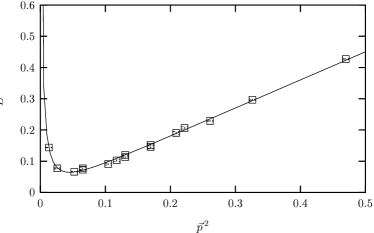
(b) $N=55,~{}\lambda=55,~{}m^{2}=-15$

Figure 7: The dispersion relation $E^{2}(\vec{p}^{\,2})$ in the disorder phase, close to the ordering transition. On the left: at weak coupling — above the uniform phase — it takes the standard shape known from the commutative world, including the lattice correction (dashed line). On the right: at strong coupling — above the striped phase — the rest energy increases and the energy minimum moves to finite momenta. The line is a four parameter fit to the one loop prediction [21, 24]. Although we are still in the disordered phase, the system already feels the trend towards a stripe formation.

If we enlarge the lattice, we expect the dispersion relation to stabilize if the axes are taken in physical units (an exception is of course the close vicinity of $\vec{p}=\vec{0}$). The required re-scaling of the axes determines the physical lattice spacing $a$. A clear hint that such a stabilization can indeed be achieved is the preliminary Fig. 8 — for the corresponding definition of the $a$ (which also stabilizes the spatial correlator) we refer to Ref. [25]. We see here in particular that the energy minimum stabilizes in physical units, which means that at large $N$ we find an infinite number of stripes with a stable average width, which can be denoted as a zebra pattern. (Of course this also includes the interference of stripes in several directions; this is what we meant by checker-field pattern.) Once this is fully demonstrated, we have established the continuum limit and the final confirmation of the existence of the striped phase, as conjectured by Gubser and Sondhi [15].

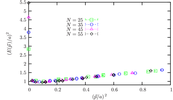
Figure 8: The dispersion relations at different sizes $N$ and physical lattice spacings $a$. The product $Na^{2}=100$ is kept constant, which corresponds to the prescription of the double scaling limit. We see that the rest energy seems to diverge at large $N$, whereas the shape of the rest of the dispersion relation stabilizes.

We finally remark that the occurrence of stripes in the lattice formulation was also observed in the case of two NC dimensions in $d=2$ [22, 20, 21] and in $d=4$ [25]. In both cases, this observation is not trivial from the theoretical point of view: since such a phase breaks the translation invariance spontaneously, one may wonder if it can possibly exist in $d=2$ at all [15], c.f. Section 2. However, there is no contradiction with the Mermin-Wagner Theorem because the proof of the latter assumes locality and an IR regular behavior, which is both not provided here. In $d=4$, on the other hand, the situation might be special because we are dealing with the critical dimension in view of the renormalization group [16], and an exciting question would be if there are any news about triviality once $\Theta$ enters the game.

4 Conclusions

We have presented results from a numerical study of the $\lambda\phi^{4}$ model in 3d Euclidean space, where the two spatial directions are NC, whereas the Euclidean time is commutative. The system was first lattice discretized and then mapped onto a dimensionally reduced matrix model. On each time lattice point one obtains a Hermitian $N\times N$ matrix, where $N\times N$ is the spatial lattice volume. We denote the physical (i.e. dimensionful) lattice space as $a$. The double scaling limit $N\to\infty$, at $Na^{2}=~{}constant$ describes the limit of an infinite volume in the continuum at a finite non-commutativity parameter $\theta$. This means that the UV limit and the thermodynamic limit are intertwined in this case, as a consequence of UV/IR mixing.

We find a phase diagram which stabilizes for $N\mathop{\raise 1.29167pt\hbox{$>$\kern-7.5pt\raise-4.73611pt\hbox{$\sim$}}}25$. The ordered regime splits into a uniform and a striped phase, which is consistent with the conjecture by Gubser and Sondhi. We discussed the order parameter, which is able to detect different types of stripe patterns. The spatial correlators in the disordered phase decay in some irregular way (fast but in general not exponential), whereas the correlators in time direction — at fixed spatial momentum — do decay exponentially. Based on the latter property we can determine the dispersion relation, which reveals the UV/IR mixing again. At large $\lambda$ the energy minimum drifts away from zero, in accordance with the occurrence of stripe patterns in the ground state. The $\Theta$-deformed dispersion relation at large $\lambda$ seems to be IR divergent. Hence the short-ranged non-locality has once again also long range manifestations.

As an outlook we hope to identify a similar dispersion relation for the photon, which would be of immediate phenomenological interest, as we outlined in Section 1. We repeat that the experimental search for bounds on $\theta$ based on a possible frequency dependence of the speed of light rely so far on a one loop calculation [11] (with an uncertain behavior at higher loops). Therefore a non-perturbative result would certainly be valuable. A first step in that direction was the study of Wilson loops in the 2d NC $U(1)$ gauge theory [26].

Acknowledgement   It is a pleasure to thank J. Ambjørn, S. Catterall, F. Iachello, D. Lüst, Y. Makeenko and R. Szabo for useful comments. The computations were performed at the PC clusters at Humboldt Universität and Freie Universität, Berlin.

References

- [1] H.S. Snyder, Phys. Rev. 71 (1947) 38.
- [2] C.N. Yang, Phys. Rev. 72 (1947) 874.
- [3] A. Connes and M. Rieffel, Contemp. Math. 62 (1987) 237.
-
[4]
A. Connes, M.R. Doublas and A. Schwarz,
JHEP 02 (1998) 003.
N. Seiberg and E. Witten, JHEP 09 (1999) 032. - [5] A. Abouelsaood, C. Callan, C.R. Nappi and S.A. Yost, Nucl. Phys. B280 (1987) 599.
-
[6]
S.M. Girvin and A.H. MacDonald, Phys. Rev. Lett.
58 (1987) 1252.
L. Susskind, hep-th/0101029.
A.P. Polychronakos, JHEP 06 (2001) 070. - [7] J.L.F. Barbon, “Introduction to noncommutative theories”, Lecture at ICTP Trieste, Summer 2001.
- [8] S. Doplicher, K. Fredenhagen and J.E. Roberts, Phys. Lett. B331 (1994) 39; Commun. Math Phys. 172 (1995) 187.
-
[9]
N. Seiberg, L. Susskind and N. Toumbas,
JHEP 0006 (2000) 044.
H. Bozkaya, P. Fischer, H. Grosse, M. Pitschmann, V. Putz, M. Schweda and R. Wulkenhaar, Eur. Phys. J. C29 (2003) 133. - [10] G. Amelino-Camelia, L. Doplicher, S. Nam and Y.-S. Seo, Phys. Rev. D67 (2003) 085008.
- [11] A. Matusis, L. Susskind and N. Toumbas, JHEP 0012 (2000) 002.
- [12] T. Filk, Phys. Lett. B376 (1996) 53.
- [13] S. Minwalla, M. van Raamsdonk and N. Seiberg, JHEP 02 (2000) 020.
- [14] R.J. Szabo, Phys. Rept. 378 (2003) 207.
- [15] S.S. Gubser and S.L. Sondhi, Nucl. Phys. B605 (2001) 395.
- [16] G.-H. Chen and Y.-S. Wu, Nucl. Phys. B622 (2002) 189.
- [17] J. Ambjørn, Y.M. Makeenko, J. Nishimura and R.J. Szabo, JHEP 05 (2000) 023.
- [18] H. Aoki, N. Ishibashi, S. Iso, H. Kawai, Y. Kitazawa and T. Tada, Nucl. Phys. B565 (2000) 176.
- [19] A. González-Arroyo and M. Okawa, Phys. Lett. 120B (1983) 174; Phys. Rev. D27 (1983) 2397.
- [20] W. Bietenholz, F. Hofheinz and J. Nishimura, Nucl. Phys. B (Proc. Suppl.) 119 (2003) 941; Fortsch. Phys. 51 (2003) 745.
- [21] F. Hofheinz, Ph.D. Thesis, Humboldt Univ. Berlin, 2003.
- [22] J. Ambjørn and S. Catterall, Phys. Lett. B549 (2002) 253.
- [23] D. Mihailovic and V.V. Kabanov, Phys. Rev. B63 (2001) 054505.
- [24] W. Bietenholz, F. Hofheinz and J. Nishimura, hep-th/0309182.
- [25] W. Bietenholz, F. Hofheinz and J. Nishimura, in preparation.
- [26] W. Bietenholz, F. Hofheinz and J. Nishimura, JHEP 09 (2002) 009.