Gravitational energy loss in high energy particle collisions: ultrarelativistic plunge into a multidimensional black hole
Abstract
We investigate the gravitational energy emission of an ultrarelativistic particle radially falling into a -dimensional black hole. We numerically integrate the equations describing black hole gravitational perturbations and obtain energy spectra, total energy and angular distribution of the emitted gravitational radiation. The black hole quasinormal modes for scalar, vector, and tensor perturbations are computed in the WKB approximation. We discuss our results in the context of black hole production at the TeV scale.
pacs:
04.70.Bw, 04.50.+hI Introduction
Brane-world models describe the visible universe as a four-dimensional brane embedded in a higher-dimensional bulk extradim . A generic consequence of the brane-world scenario is that the fundamental gravitational scale is lower than the observed Planck scale. In some models, the fundamental scale is lowered to values that would be accessible to next-generation particle colliders, thus enabling laboratory-based studies of strong gravitational physics via perturbative pertextradim and nonperturbative events nonpertextradim . Ultrahigh energy cosmic rays could also probe trans-Planckian energies uhecr . The possibility that strong gravitational effects such as black hole (BH) and brane formation could be observed in the near future has sparked a lot of interest in the investigation of nonperturbative gravitational phenomena in hard-scattering events hardscat . (For a review and more references, see Ref. Cavaglia:2002si ).
Trans-Planckian BH formation at energy scales much larger than the fundamental gravitational scale is a classical process nonpertextradim . The event is dominated by the -channel and the initial state is modelled by two classical shock waves with given impact parameter. In this context, a major issue is the estimate of the collisional energy loss. The hoop conjecture states that the collision of two particles with center-of-mass (c.m.) energy and impact parameter smaller than the Schwarzschild radius forms a trapped surface hoop . This event is formally described by the process , where denotes the collisional “junk” energy which does not contribute to the BH mass. The junk energy includes a bulk component of gravitational radiation and other possible non-standard model gauge fields, and a brane component of standard model collisional by-products carrying the charge of the initial particles. The newly formed BH is expected to decay first by loss of gauge radiation into the bulk and then by thermal Hawking emission. The Hawking evaporation ends when the mass of the BH approaches the fundamental gravitational scale. At this stage the BH either decays completely by emitting the residual Planckian energy or leaves a stable remnant with mass about the Planck mass relic . Most of the observable signatures of BH formation come from Hawking’s phase and strongly depend on the initial BH mass Cavaglia:2003hg . Hence, a precise calculation of the collisional energy loss is essential to the phenomenology of BH formation.
A numerical estimate of the total collisional energy loss for spherically symmetric BHs in dimensions has been given by Yoshino and Nambu (YN) Yoshino:2002tx (see also Ref. Vasilenko:2003ak ). The YN approach evaluates the total junk energy by investigating the formation of the BH apparent horizon apphor . The colliding particles are assumed massless, uncharged and pointlike. Each particle is modelled by an infinitely boosted Schwarzschild solution with fixed energy. This solution describes a plane-fronted gravitational shock wave corresponding to the Lorentz-contracted longitudinal gravitational field (Aichelburg-Sexl wave) Aichelburg:1970dh . The collision is simulated by combining two shock waves travelling in opposite directions. The apparent horizon arises in the union of the two shock waves. The junk energy is estimated by comparing the initial c.m. energy to the BH mass. The result is that the collisional energy loss depends on the impact parameter and increases as the number of spacetime dimensions increases.
The YN method allows estimation of the total junk energy in the classical uncharged point-particle approximation. However, it cannot discriminate between different components of , which is theoretically and experimentally most important. In a realistic BH event such as a proton-proton collision at LHC LHC , the BH is formed by the collision of two partons. The bulk component of the junk energy is dominated by gravitational radiation and is invisible to the detector. The gravitational junk energy and the invisible component of Hawking emission (neutrinos, gravitons …) add to the total missing energy of the process. Therefore, the knowledge of collisional energy loss in gravitational emission should provide a good estimate of the different sources of energy loss and missing energy.
An accurate estimate of the gravitational collisional energy loss would require the use of the full non-linear Einstein equations in dimensions. This is a formidable task, even in four dimensions. Recently, significant advances in numerical relativity allowed stable numerical simulations of BH-BH collisions for initial BH separation of a few Schwarzschild radii in the non-linear Einstein theory. The gravitational waveforms predicted by these simulations are in excellent agreement with analytical results from first and second order perturbation theory Gleiser:1998rw . Since the linearization of the Einstein equations yields results which are surprisingly close to the full theory (see, e.g., Ref. Anninos:1998wt ), BH perturbation theory is likely to provide accurate estimates of gravitational wave emission in higher-dimensional spacetimes. Relying on this result, we compute the gravitational wave emission in higher dimensions via a perturbative approach. Our computation is the first of this kind to our knowledge.
The formalism for the computation of gravitational wave emission from perturbed BHs was developed by Regge and Wheeler RW and Zerilli Zerilli , who reduced the problem to the solution of two Schrödinger-like equations. Davis et al. DRPP computed the energy radiated in the radial infall of a particle of mass starting from rest at infinity into a four-dimensional BH of mass . This study was later generalized to the radial infall of a particle with finite initial velocity or starting at finite distance from the BH Ruffini . (For a more comprehensive introduction to BH perturbation theory see, e.g., Refs. perturb ). Cardoso and Lemos Cardoso:2002ay ; Cardoso:2002yj have recently investigated the plunge of ultrarelativistic test particles into a four-dimensional static BH and along the rotation axis of a Kerr BH, improving early estimates by Smarr Smarr:1977 . In this paper we generalize these results to higher dimensions by computing the gravitational radiation emitted by an ultrarelativistic particle falling into a -dimensional spherically symmetric BH. Since wave propagation in odd-dimensional curved spacetimes is not yet fully understood, we restrict our investigation to even dimensions. (Wave late-time behavior and propagation are very different in odd- and even-dimensional spacetimes Cardoso:2002pa ; Cardoso:2003jf ; Barvinsky:2003jf . Moreover, open issues in the definition of asymptotic flatness Hollands:2003ie do not allow an unambiguous definition of “gravitational waves radiated at infinity” in odd dimensions.)
We model the particle collision as a relativistic test particle plunging into a BH with mass . We use recent results of -dimensional gravitational-wave theory by Cardoso et al. Cardoso:2002pa and the -dimensional extension of Zerilli’s formalism by Kodama and Ishibashi (KI) Kodama:2000fa ; Kodama:2003jz ; Ishibashi:2003ap ; Kodama:2003kk , which reduces the problem to the solution of three Schrödinger-like equations. Our method provides a simple and relativistically consistent estimate of the collisional gravitational emission in higher dimensions. We derive the emitted energy in terms of the wave amplitude and study the angular dependence of the radiation using the KI formalism. We also present a systematic calculation of BH quasinormal modes (QNMs) for the different perturbations in the WKB approach, extending recent calculations by Konoplya Konoplya:2003ii ; Konoplya:2003dd . We show that there is a significant relation between the QNM frequencies and the spectral content of the emitted radiation.
The outline of the paper is as follows. In Sec. II we introduce our notations and the basic equations. In Sec. III we briefly describe our numerical approach to the computation of gravitational wave emission (details are in the Appendices). Section IV contains the main results of the paper. Conclusions are presented in Sec. V.
II Perturbation equations and quasinormal modes
In the next subsection we introduce the background metric and the KI perturbation equations Kodama:2003jz . In Subsec. II.2 we describe the method to compute the BH QNMs.
II.1 Background metric and perturbation equations
The spherically symmetric BH in dimensions is described by the Schwarzschild-Tangherlini metric Tangherlini:1963
| (1) |
where is the metric of the -dimensional unit sphere , and
| (2) |
The BH mass is given in terms of the parameter by
| (3) |
where is the area of , is the -dimensional Newton constant, and is the speed of light. We will set and in the following. The -dimensional tortoise coordinate is defined by
| (4) |
Integrating Eq. (4) we find
| (5) |
where
| (6) |
and the integration constant has been chosen to make the argument of the logarithm dimensionless. Here and throughout the paper we use the notations of Refs. Kodama:2003jz ; Kodama:2000fa ; the indices , , and denote the coordinates of the -dimensional spacetime, the coordinates of , and the coordinates of the two-dimensional spacetime , respectively.
Kodama and Ishibashi Kodama:2003jz showed that the gravitational perturbation equations for this metric can be reduced to Schrödinger–like wave equations:
| (7) |
where the potential depends on the kind of perturbation. Setting , the potential for scalar perturbations is
| (8) |
where
| (9) |
and
| (10) | |||||
Equation (8) reduces to the Zerilli equation Zerilli for . The potential for vector perturbations is
| (11) |
where
| (12) |
Equation (11) reduces to the Regge-Wheeler equation RW for . Finally, the potential for tensor perturbations is
| (13) |
where
| (14) |
Equation (13) was derived by Gibbons and Hartnoll Gibbons:2002pq in a more general case (see also Neupane , where a Gauss-Bonnet term is included) and has no equivalent in four dimensions.
II.2 Quasinormal modes
The knowledge of the QNM frequencies of multidimensional BHs enables a clear physical interpretation of their gravitational emission. QNMs are free damped BH oscillations which are characterized by pure ingoing radiation at the BH horizon and pure outgoing radiation at infinity. The no-hair theorem implies that QNM frequencies depend only on the BH mass, charge and angular momentum. Numerical simulations of BH collapse and BH-BH collision show that, after a transient phase depending on the details of the process, the newly formed BH has a ringdown phase, i.e., it undergoes damped oscillations that can be described as a superposition of slowly damped QNMs (modes with small imaginary part). Furthermore, the QNMs determine the late-time evolution of perturbation fields in the BH exterior (for comprehensive reviews on QNMs see Refs. KS ).
Gravitational radiation from four-dimensional astrophysical BHs is dominated by slowly damped modes. In the following we show that these also dominate the emission of gravitational radiation in higher dimensions and determine important properties of the energy spectra. Recently, Konoplya computed slowly damped QNMs of higher-dimensional BHs Konoplya:2003ii ; Konoplya:2003dd using the WKB method. This method is known to be inaccurate for large imaginary parts, but it is accurate enough for the slowly damped modes which are relevant in our context. Therefore, QNM frequencies for scalar, vector, and tensor gravitational perturbations are computed here in the WKB approximation. Our results are in good agreement with those presented by Konoplya in Ref. Konoplya:2003dd (modulo a different normalization). At variance with Ref. Konoplya:2003dd , we concentrated on uncharged black holes in asymptotically flat, even dimensional spacetimes. We extended Konoplya’s calculation in two ways: i) in addition to the fundamental QNM we also computed the first two overtones; ii) we carried out our calculations for a much larger range of values of (Ref. Konoplya:2003dd only shows results for and ).
The method consists in applying the WKB approximation to the potential in Eq. (7) with appropriate boundary conditions. The result is a pair of connection formulae which relate the amplitudes of the waves on either side of the potential barrier, and ultimately yield an analytical formula for the QNM frequencies (for details see Refs. Iyer:np ; Iyer:nq ). The WKB QNM frequencies are given in terms of the potential maximum and of the potential derivatives at the maximum by
| (15) |
where
| (16) | |||||
and is the mode index. The QNM frequencies for the scalar, vector, and tensor potentials of Sec. II and various dimensions are shown in Tables 1-4 and will be discussed in Sec. IV. Let us stress that the application of the WKB technique is questionable in a few higher-dimensional cases; for and the vector and scalar potentials in are not positive definite and/or display a second, small scattering peak close to the BH horizon. An accurate analysis of these potentials would require a refinement of the standard WKB technique, which is not presented here. These special cases are denoted with italic numbers in Tables 3-4.
We mention that highly damped QNMs of four- and higher-dimensional BHs have recently become a subject of great interest in a different context. A few years ago, Hod proposed to use Bohr’s correspondence principle to determine the BH area quantum from highly damped BH QNMs Hod:1998vk . Hod’s proposal is quite general: the asymptotic QNM frequency for scalar perturbations of a non-rotating BH in dimensions is the same as in four dimensions Motl:2003cd . Quite notably, this result holds also for scalar, vector and tensor gravitational perturbations Birmingham:2003rf ; Motl:2003cd . Ref. AreaQuantum contains a partial list of references on recent developments in this field.
III Integration method
The computation of the gravitational wave emission of an ultrarelativistic particle plunging into a BH requires the numerical integration of the inhomogeneous wave equation for scalar gravitational perturbations. (Vector and tensor gravitational perturbations are not excited by a particle in radial infall.) The source term for the corresponding wave equation in dimensions can be calculated from the stress-energy tensor of the infalling particle. Details of the derivation are in Appendix A.
The integration in dimensions proceeds as in four dimensions DRPP ; Ruffini . A good summary of the integration procedure can be found in Ref. Cardoso:2002ay . In this section we simply stress the differences between the four- and the -dimensional cases. For the sake of simplicity, in our numerical integrations we set the horizon radius . The equation for the scalar perturbations is
| (18) |
The general solution of Eq. (18) is obtained via a Green function technique as follows. Consider two independent (left and right) solutions of the homogeneous equation with boundary conditions for , and for . For the left solution is a superposition of ingoing and outgoing waves of the form
| (19) |
The Wronskian is given by . The wave amplitude is obtained from a convolution of the left solution with the source term
| (20) |
The energy spectrum can be expressed in terms of the wave amplitude as (details of the derivation are given in Appendix B)
| (21) |
where . The Wronskian for a given value of is obtained by integrating the homogeneous equation from a point located as close as possible to the horizon, and expanding as
| (22) |
where
| (23) |
(and ) can be obtained with good accuracy by matching the numerically integrated to the asymptotic expansion
| (24) |
where the leading-order coefficient is
| (25) |
For given , and , the error on the Wronskian and on the energy spectrum is typically of the order of .
IV Results
The main results of our work are the computation of the QNM frequencies in the WKB approximation, the computation of the energy spectra, and the estimate of the total energy and angular distribution of the radiation emitted during the plunge. These results are discussed in detail below.
IV.1 Quasinormal frequencies
The WKB QNM frequencies for different even values of are listed in Tables 1-4. Each line shows the first three quasinormal frequencies () for scalar, vector, and tensor perturbations at given . For tensor perturbations do not exist. In this case the scalar and vector entries correspond to the QNMs of the Zerilli and Regge-Wheeler equations, which are known to be isospectral perturb . The isospectrality is broken for . This has been shown analytically by Kodama and Ishibashi Kodama:2003jz and later verified numerically by Konoplya Konoplya:2003dd . The real and imaginary parts of scalar QNM frequencies at given , and are smaller than those of vector QNMs, which are in turn smaller than those of tensor QNMs. Since scalar modes are the least damped, they are likely to dominate the gravitational radiation emission.
As grows, the isospectrality tends to be restored. In the eikonal limit the centrifugal term of the potential dominates and is the same for scalar, vector, and tensor perturbations. In this limit, the QNM frequencies for all perturbations are
| (26) |
The previous relation was derived in Ref. Konoplya:2003ii for multidimensional BH perturbations induced by a scalar field. (Notice that the normalization used in Ref. Konoplya:2003ii is different from ours.) Here we have shown that it also holds for gravitational perturbations. Isospectrality of scalar and gravitational perturbations is a common feature of the eikonal limit and of the large-damping limit Birmingham:2003rf ; Motl:2003cd for any .
IV.2 Multipolar components of the energy spectra
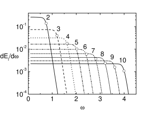
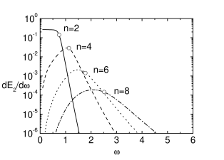
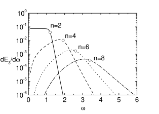
The numerical integration described in Sec. III gives the energy spectra of Figs. 1 and 2. The spectra for (top left panel in Fig. 1) are in excellent agreement with those of Ref. Cardoso:2002ay . The spectra are flat in the region between the zero-frequency limit and a “cutoff” frequency , beyond which they fall exponentially to zero. The cutoff frequency is given by the fundamental QNM frequency to a good level of accuracy. This result can be understood in terms of gravitational-wave scattering from the potential barrier which surrounds the black hole. plays the role of the energy in the Schrödinger-like equation (7). From Eq. (15) it follows that at first order in the WKB approximation. Therefore, only the radiation with energy smaller than the peak of the potential is backscattered to infinity; radiation with larger frequency is exponentially suppressed.
The gravitational emission of a two-particle hard collision in higher dimensions has been computed by Cardoso et al. Cardoso:2002pa using techniques developed in four dimensions by Weinberg Weinberg and later used by Smarr Smarr:1977 . The main result of Ref. Cardoso:2002pa is that the spectra in dimensions grow as , thus the integrated spectra diverge as . Physically meaningful results for the total energy can only be obtained by imposing some cutoff on the integrated spectra. Smarr Smarr:1977 first suggested to use the inverse horizon radius as a cutoff. The relativistic perturbative calculation in Cardoso:2002ay shows that the cutoff frequency at fixed is very close to the fundamental BH QNM. Therefore, the cutoff frequency should be given by some “weighted average” of the fundamental gravitational QNM frequencies Cardoso:2002pa .
Our results for the spectra and the QNMs confirm the above picture. Fig. 1 shows that all spectra go to zero as . For the spectrum at fixed is
| (27) |
where is a constant that can be found by a fit of the spectra. For large decays as
| (28) |
A fit of the numerical data gives , , , and . Our result for is consistent with that of Ref. Cardoso:2002ay .
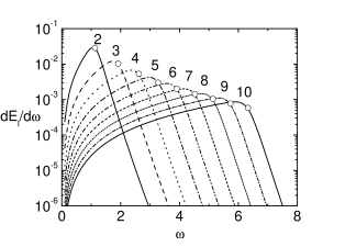
As conjectured in Ref. Cardoso:2002pa , all spectra have a maximum at some cutoff frequency . This cutoff frequency is very close to the fundamental QNM frequency for (scalar) gravitational perturbations with given and , which is marked by open circles in Fig. 1 and Fig. 2. The deviation between and is of order 10 % for low , and decreases for large (compare Fig. 1 and Fig. 2 to the first column of Tables 1-4). The deviation is larger when the WKB method is least reliable, namely for and . In these cases, the location of the peaks in the spectra can presumably be used as a more reliable estimate of the QNM frequency. The spectrum decays exponentially for with an -dependent slope (see Fig. 2):
| (29) |
Thus the -integrated multipolar contributions at given are finite. With our choice of units, Cardoso and Lemos Cardoso:2002ay find (here is a constant of order unity which cannot easily be determined because the spectra decay very quickly). Our numerical fits give , in good agreement with their result. In higher dimensions the constants are comparatively easier to determine. Their values are , , and . It is not clear if there is any relation between this -dependent slope and the late-time tail behavior predicted in Ref. Cardoso:2003jf .
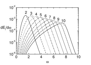
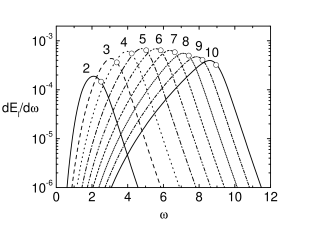
Fig. 1 shows that higher multipoles contribute more as grows. This is evident when we look at the -integrated multipolar components of the energy spectra of Fig. 3. The quadrupole () is dominant only for and . For and the dominant multipoles are and , respectively (see Table 5). This effect may be related to the appearance of a negative well in the scalar potentials for and . It would be interesting to understand better the physical relation between the dominant multipole and the spacetime dimension.
IV.3 Total energy
The total emitted energy is obtained by numerically integrating the results of the previous section over and summing the multipolar components. For large the integrated energy in the multipole can be fitted by
| (30) |
where , , and for , , and , respectively. The coefficients have been obtained by fitting the data from to and are weakly dependent on the chosen range of . This variability affects our final results on the total energy within less than a few percent.
Restoring the dependence on the BH horizon and on the conserved particle energy , the total emitted energy is
| (31) |
where is the “dimensionless” total energy (expressed in the units that we used in our numerical integrations). We obtained the integrated spectra numerically up to and extrapolated them for larger using the fits in Eq. (30). Results are presented in Table 6.
Following Ref. Cardoso:2002ay we estimate the gravitational energy loss for a collision of two particles with equal mass by the replacement , . For this extrapolation gives results in good agreement with the perturbative shock-wave calculation of Ref. apphor which considers two BHs of equal mass. An analogous extrapolation for gives results in close agreement with the fully relativistic computation Anninos:1998wt for a particle starting from infinity at rest. Therefore, we believe that our extrapolation should provide a qualitative but realistic estimate. The results for different values of are given in the last column of Table 6. The gravitational energy loss is %, %, %, and % for to , respectively. The result for is in good agreement with previous estimates apphor (see the discussion in Ref. Cardoso:2002ay ).
IV.4 Angular dependence
The angular dependence of the radiation is obtained by evaluating numerically Eq. (67) and Eq. (68). Fig. 4 shows the angular dependence of the total energy up to for , and .
The angular distribution of the gravitational radiation in the BH frame goes to zero along the axis of the collision (, ) in any dimensions. Therefore, the gravitational emission is never back or forward scattered. In four dimensions the angular spectrum of the gravitational radiation increases rapidly at small and becomes approximately flat at greater angles with a maximum in the direction orthogonal to the axis of the collision, before falling rapidly to zero for values of the angles close to . The angular distribution of the gravitational radiation for is peaked at and , where is a small angle. The difference between the behavior of the angular distribution in four dimensions and in higher dimensions has no evident physical reason. It would be interesting to further explore this point.
V Conclusion and perspectives
In this paper we have computed the gravitational emission of a two-particle collision in an even -dimensional spacetime. We have presented the numerical results for to . The collision has been modelled as a massless test particle plunging into a BH with mass equal to the c.m. energy of the event.
According to our estimates, the total emitted energy in a head-on collision with particles of equal mass ranges from % () to % (). This shows that the loss in gravitational radiation is quite stable under variation of the spacetime dimension and slightly decreases for higher . The result for confirms previous numerical and analytical calculations apphor .
Our result contrasts with the YN estimation for the initial mass of a BH in head-on collisions Yoshino:2002tx . A possible explanation is that the junk emission is not wholly gravitational emission. The YN method predicts the mass within the apparent horizon to be in four dimensions. If all the junk energy were gravitational radiation, this would amount to a total loss of around %. The disagreement is likely not due to numerical uncertainties or inaccurate approximations: the YN mass decreases for higher spacetime dimensions ( to for to ), whereas the loss in gravitational radiation remains stable. Since both YN and our methods are purely gravitational, this “dark component” of the junk radiation should describe the by-products of the collision. According to this picture, % of the c.m. energy in ten dimensions is trapped inside the horizon, % is emitted in gravitational radiation, and % goes into particle by-products in the final state. These could be the carriers of the initial charge in a collision between charged particles. For a fraction of the by-products may be emitted into the bulk.
Let us conclude by briefly discussing the phenomenological consequences of these results for BH formation at the TeV scale. Although uncertainties may affect the numerical estimates, different approaches now confirm that some of the initial c.m. energy is not trapped inside the BH horizon. For head-on collisions in , for example, this junk energy ranges from % (optimistic value – our result) to % (pessimistic value – YN result). Hence, the initial mass of the BH formed in the collision could be considerably smaller than the c.m. energy. The experimental signatures of BH production at particle colliders and in ultrahigh energy cosmic ray events strongly depend on the initial BH mass. The total multiplicity of the Hawking phase in ten dimensions could be almost halved in the pessimistic case, leading to a greater average energy of the emitted quanta.
A thorough investigation of the effects of energy loss in TeV-scale BH production is undoubtedly worth pursuing. Future research should focus on the extension of the above results to spacetimes with odd dimensions and to gravitational events with different geometries. BHs produced in colliders, for instance, possess nonvanishing angular momentum. Rotating BHs are expected to lose more energy in gravitational waves than Schwarzschild BHs of equal mass. A larger gravitational emission is also expected for non-spherically symmetric BHs. This is particularly relevant when the compactified space is asymmetric, and some of the extra dimensions have size of order of the fundamental gravitational scale. It would be extremely important to quantify these differences.
Acknowledgements.
We warmly thank V. Cardoso for his encouragement to carry out this work and for several useful suggestions. M. C. is grateful to E.-J. Ahn for many helpful comments on the content of this paper. This work has been supported by the EU Programme ‘Improving the Human Research Potential and the Socio-Economic Knowledge Base’ (Research Training Network Contract HPRN-CT-2000-00137). M. C. is partially supported by PPARC.Appendix A The source term
In this Appendix we derive the source term of the KI equation that describes the radial plunge of a massless particle into the -dimensional BH. The perturbation of the stress-energy tensor is
| (32) |
where is the conserved energy of the particle. The only non-vanishing components of the particle velocity are and . Thus the source excites only scalar perturbations. Following the notations of Ref. Kodama:2000fa , Eq. (32) reads
| (33) |
where are the scalar harmonics and are the non-vanishing gauge-invariant perturbations of the stress-energy tensor. The BH+source system is symmetric under rotation of the -sphere Cardoso:2002cf . Consequently, the harmonic decomposition of the fields contains only harmonics invariant under . We can write the metric of as
| (34) |
and choose the trajectory of the test particle to be . The harmonics which are invariant under do not depend on . The scalar harmonics on belong to the representations of
| (35) |
Each harmonic is labelled by the index denoting its representation and by additional indices in the representation. We fix a particular element of each representation (the singlet under ) by requiring the harmonics to be invariant under . Therefore, the harmonics in the expansion of the perturbations depend only on and on the dimension of the sphere. A -dimensional scalar field can then be expanded as Cardoso:2002cf
| (36) |
where satisfy
| (37) |
and
| (38) |
The solution of Eq. (37) is
| (39) |
where are Gegenbauer polynomials Abr and are normalization factors. Using Eq. (38) we have
| (40) |
The scalar harmonics for the source are obtained setting :
| (41) |
For a massive particle in radial geodesic motion
| (42) |
From equations (42) and (4) it follows that
| (43) |
where we have set to zero the integration constant. The stress-energy tensor perturbations are
| (44) |
( does not contribute to the source of the KI equation.) Integrating Eqs. (A) on and applying a Fourier-transform, the gauge-invariant perturbations are
| (45) |
The source term for scalar gravitational perturbations is obtained in terms of by substituting Eqs. (45) in Eq. (5.44) of Ref. Kodama:2003kk , where
| (46) |
The result is:
| (47) | |||||
| (48) | |||||
| (49) | |||||
| (50) |
where . The BH horizon and the particle energy have been set equal to one. Equation (47) coincides with Eq. (8) of Ref. Cardoso:2002ay .
Appendix B Energy and angular distribution
We derive here the formulae for the energy and the angular dependence of the gravitational emission. Gravitational waves in a -dimensional spacetime behave asymptotically as Cardoso:2002pa and possess degrees of freedom. The transverse-traceless (TT) gauge is defined by , , and . These conditions can be chosen by imposing the harmonic gauge in the wave zone and using the remaining gauge freedom to constrain , , and .
We separate the angular part of the perturbations using tensor spherical harmonics, following Ref. Kodama:2003jz . In the TT-gauge, the only nonvanishing term in the decomposition is the component. Hence, the gauge invariant quantities for scalar perturbations ( and ) depend only on :
| (51) |
where
| (52) |
The scalar perturbation is written in terms of the gauge invariant quantities as
| (53) |
where
| (54) |
Setting
| (55) |
the asymptotic behavior of is
| (56) |
The asymptotic behavior of in the TT-gauge is
| (57) |
The energy-momentum pseudotensor does not depend on the spacetime dimension and is given by Cardoso:2002pa
| (58) |
where are metric perturbations in the time domain. Using Parseval’s theorem, the energy-momentum pseudotensor in the frequency domain is
| (59) |
where are now the metric perturbations in the frequency domain. Substituting Eq. (57) in Eq. (59) we get
| (60) |
Integrating on the sphere and using the relations
| (61) |
where is a generic vector (here and in the following, indices are raised and lowered with ), we find the “two-sided” power spectrum
| (62) |
The “one-sided” spectrum in Eq. (21) is obtained by multiplying Eq. (62) by two. In the four-dimensional limit the one-sided spectrum is
| (63) |
Equation (63) is Zerilli’s formula for the -th multipole component of the energy spectrum in four-dimensions. The total energy spectrum is given by the sum over the multipoles.
For each the energy spectrum is
| (64) |
Substituting Eq. (62) in the previous equation, we find
| (65) |
The angular dependence for the -th multipole is obtained by integrating over frequency Cardoso:2002ay . The result is
| (66) |
where
| (67) |
For Eq. (67) reduces to the known result in four dimensions Cardoso:2002ay . The angular dependence is obtained by summing over the multipoles:
| (68) |
The result truncated to is shown in the left panel of Fig. 4. The curve corresponding to shows good agreement with Fig. 3 of Ref. Cardoso:2002ay .
References
- (1) I. Antoniadis, Phys. Lett. B 246, 377 (1990); N. Arkani-Hamed, S. Dimopoulos and G. R. Dvali, Phys. Lett. B 429, 263 (1998) [arXiv:hep-ph/9803315]; I. Antoniadis, N. Arkani-Hamed, S. Dimopoulos and G. R. Dvali, Phys. Lett. B 436, 257 (1998) [arXiv:hep-ph/9804398]; L. Randall and R. Sundrum, Phys. Rev. Lett. 83, 3370 (1999) [arXiv:hep-ph/9905221]; L. Randall and R. Sundrum, Phys. Rev. Lett. 83, 4690 (1999) [arXiv:hep-th/9906064].
- (2) G. F. Giudice, R. Rattazzi and J. D. Wells, Nucl. Phys. B 544, 3 (1999) [arXiv:hep-ph/9811291]; T. Han, J. D. Lykken and R. J. Zhang, Phys. Rev. D 59, 105006 (1999) [arXiv:hep-ph/9811350]; J. L. Hewett, Phys. Rev. Lett. 82, 4765 (1999) [arXiv:hep-ph/9811356]; T. G. Rizzo, Phys. Rev. D 59, 115010 (1999) [arXiv:hep-ph/9901209].
- (3) T. Banks and W. Fischler, arXiv:hep-th/9906038; S. B. Giddings and S. Thomas, Phys. Rev. D 65, 056010 (2002) [arXiv:hep-ph/0106219]; S. Dimopoulos and G. Landsberg, Phys. Rev. Lett. 87, 161602 (2001) [arXiv:hep-ph/0106295]; S. Dimopoulos and R. Emparan, Phys. Lett. B 526, 393 (2002) [arXiv:hep-ph/0108060]; R. Casadio and B. Harms, Int. J. Mod. Phys. A 17, 4635 (2002) [arXiv:hep-th/0110255]; E. J. Ahn, M. Cavaglià and A. V. Olinto, Phys. Lett. B 551, 1 (2003) [arXiv:hep-th/0201042].
- (4) J. L. Feng and A. D. Shapere, Phys. Rev. Lett. 88, 021303 (2002) [arXiv:hep-ph/0109106]; A. Ringwald and H. Tu, Phys. Lett. B 525, 135 (2002) [arXiv:hep-ph/0111042]; E. J. Ahn, M. Ave, M. Cavaglià and A. V. Olinto, Phys. Rev. D 68, 043004 (2003) [arXiv:hep-ph/0306008].
- (5) S. Hossenfelder, S. Hofmann, M. Bleicher and H. Stocker, Phys. Rev. D 66, 101502 (2002) [arXiv:hep-ph/0109085]; K. Cheung, Phys. Rev. Lett. 88, 221602 (2002) [arXiv:hep-ph/0110163]; S. I. Dutta, M. H. Reno and I. Sarcevic, Phys. Rev. D 66, 033002 (2002) [arXiv:hep-ph/0204218]; K. Cheung, Phys. Rev. D 66, 036007 (2002) [arXiv:hep-ph/0205033]; E. J. Ahn and M. Cavaglià, Gen. Rel. Grav. 34, 2037 (2002) [arXiv:hep-ph/0205168].; V. Frolov and D. Stojkovic, Phys. Rev. D 66, 084002 (2002) [arXiv:hep-th/0206046]; T. Han, G. D. Kribs and B. McElrath, Phys. Rev. Lett. 90, 031601 (2003) [arXiv:hep-ph/0207003]; V. Frolov and D. Stojkovic, Phys. Rev. Lett. 89, 151302 (2002) [arXiv:hep-th/0208102]; I. Mocioiu, Y. Nara and I. Sarcevic, Phys. Lett. B 557, 87 (2003) [arXiv:hep-ph/0301073]; A. Chamblin, F. Cooper and G. C. Nayak, arXiv:hep-ph/0301239.
- (6) M. Cavaglià, Int. J. Mod. Phys. A 18, 1843 (2003) [arXiv:hep-ph/0210296].
- (7) K.S. Thorne, in: Magic without magic: John Archibald Wheeler, edited by J. Klauder (freeman, San Francisco, 1972).
- (8) M. Cavaglià, S. Das and R. Maartens, Class. Quant. Grav. 20, L205 (2003) [arXiv:hep-ph/0305223]; S. Hossenfelder, M. Bleicher, S. Hofmann, H. Stocker and A. V. Kotwal, arXiv:hep-ph/0302247.
- (9) M. Cavaglià, Phys. Lett. B 569, 7 (2003) [arXiv:hep-ph/0305256].
- (10) H. Yoshino and Y. Nambu, Phys. Rev. D 67, 024009 (2003) [arXiv:gr-qc/0209003].
- (11) O. I. Vasilenko, arXiv:hep-th/0305067.
- (12) P. D. D’Eath and P. N. Payne, Phys. Rev. D 46, 658 (1992); P. D. D’Eath and P. N. Payne, Phys. Rev. D 46, 675 (1992); P. D. D’Eath and P. N. Payne, Phys. Rev. D 46, 694 (1992); D. M. Eardley and S. B. Giddings, Phys. Rev. D 66, 044011 (2002) [arXiv:gr-qc/0201034]; H. Yoshino and Y. Nambu, Phys. Rev. D 66, 065004 (2002) [arXiv:gr-qc/0204060]; D. Ida and K. I. Nakao, Phys. Rev. D 66, 064026 (2002) [arXiv:gr-qc/0204082]. O. I. Vasilenko, arXiv:hep-th/0305067.
- (13) P. C. Aichelburg and R. U. Sexl, Gen. Rel. Grav. 2, 303 (1971).
- (14) http://lhc-new-homepage.web.cern.ch/lhc-new-homepage/
- (15) R. J. Gleiser, C. O. Nicasio, R. H. Price and J. Pullin, Phys. Rept. 325, 41 (2000) [arXiv:gr-qc/9807077].
- (16) P. Anninos and S. Brandt, Phys. Rev. Lett. 81, 508 (1998) [arXiv:gr-qc/9806031].
- (17) T. Regge, J. A. Wheeler, Phys. Rev. 108, 1063 (1957).
- (18) F. Zerilli, Phys. Rev. D 2, 2141 (1970).
- (19) M. Davis, R. Ruffini, W. H. Press, R. H. Price, Phys. Rev. Lett. 27, 1466 (1971).
- (20) R. Ruffini, Phys. Rev. D 7, 972 (1973); R. Ruffini, V. Ferrari, Phys. Lett. B 98, 381 (1981); C. Lousto, R. H. Price, Phys. Rev. D 55, 2124 (1997).
- (21) J. Baker, B. Brugmann, M. Campanelli, C. O. Lousto and R. Takahashi, Phys. Rev. Lett. 87, 121103 (2001) [arXiv:gr-qc/0102037]; Y. Mino, M. Sasaki, M. Shibata, H. Tagoshi and T. Tanaka, Prog. Theor. Phys. Suppl. 128, 1 (1997) [arXiv:gr-qc/9712057]; S. Chandrasekhar, The Mathematical Theory of Black Holes, Oxford University Press (1983).
- (22) V. Cardoso and J. P. Lemos, Phys. Lett. B 538, 1 (2002) [arXiv:gr-qc/0202019].
- (23) V. Cardoso and J. P. Lemos, Gen. Rel. Grav. 35, 327 (2003) [arXiv:gr-qc/0207009].
- (24) L. Smarr, Phys. Rev. D 15, 2069 (1977).
- (25) V. Cardoso, O. J. Dias and J. P. Lemos, Phys. Rev. D 67, 064026 (2003) [arXiv:hep-th/0212168].
- (26) V. Cardoso, S. Yoshida, O. J. Dias and J. P. Lemos, arXiv:hep-th/0307122.
- (27) A. O. Barvinsky and S. N. Solodukhin, arXiv:hep-th/0307011.
- (28) S. Hollands and A. Ishibashi, arXiv:gr-qc/0304054.
- (29) H. Kodama, A. Ishibashi and O. Seto, Phys. Rev. D 62, 064022 (2000) [arXiv:hep-th/0004160].
- (30) H. Kodama and A. Ishibashi, arXiv:hep-th/0305147.
- (31) A. Ishibashi and H. Kodama, arXiv:hep-th/0305185.
- (32) H. Kodama and A. Ishibashi, arXiv:hep-th/0308128.
- (33) R. A. Konoplya, Phys. Rev. D 68, 024018 (2003) [arXiv:gr-qc/0303052].
- (34) R. A. Konoplya, Phys. Rev. D 68, 124017 (2003) [arXiv:hep-th/0309030].
- (35) F. R. Tangherlini, Nuovo Cimento 27, 636 (1963).
- (36) G. Gibbons and S. A. Hartnoll, Phys. Rev. D 66, 064024 (2002) [arXiv:hep-th/0206202].
- (37) I. P. Neupane, arXiv:hep-th/0302132.
- (38) K. D. Kokkotas and B. G. Schmidt, Living Rev. Rel. 2, 2 (1999) [arXiv:gr-qc/9909058]; H.-P. Nollert, Class. Quant. Grav. 16, R159 (1999).
- (39) S. Iyer and C. M. Will, Phys. Rev. D 35, 3621 (1987).
- (40) S. Iyer, Phys. Rev. D 35, 3632 (1987).
- (41) S. Hod, Phys. Rev. Lett. 81, 4293 (1998) [arXiv:gr-qc/9812002].
- (42) L. Motl and A. Neitzke, arXiv:hep-th/0301173.
- (43) D. Birmingham, arXiv:hep-th/0306004.
- (44) O. Dreyer, Phys. Rev. Lett. 90, 081301 (2003) [arXiv:gr-qc/0211076]; G. Kunstatter, Phys. Rev. Lett. 90, 161301 (2003) [arXiv:gr-qc/0212014]; L. Motl, Adv. Theor. Math. Phys. 6, 1135 (2003) [arXiv:gr-qc/0212096]; E. Berti and K. D. Kokkotas, Phys. Rev. D 67, 064020 (2003) [arXiv:gr-qc/0301052]; V. Cardoso and J. P. Lemos, Phys. Rev. D 67, 084020 (2003) [arXiv:gr-qc/0301078]; C. Molina, Phys. Rev. D 68, 064007 (2003) [arXiv:gr-qc/0304053]; A. Neitzke, arXiv:hep-th/0304080; A. Maassen van den Brink, Phys. Rev. D 68, 047501 (2003) [arXiv:gr-qc/0304092]; V. Cardoso, R. Konoplya and J. P. Lemos, Phys. Rev. D 68, 044024 (2003) [arXiv:gr-qc/0305037]; D. Birmingham, S. Carlip and Y. j. Chen, arXiv:hep-th/0305113; E. Berti, V. Cardoso, K. D. Kokkotas and H. Onozawa, arXiv:hep-th/0307013; N. Andersson and C. J. Howls, arXiv:gr-qc/0307020; S. Hod, arXiv:gr-qc/0307060; S. Yoshida and T. Futamase, arXiv:gr-qc/0308077; S. Musiri and G. Siopsis, arXiv:hep-th/0308168. J. Oppenheim, arXiv:gr-qc/0307089.
- (45) S. Weinberg, Gravitation and Cosmology (Wiley, New York, 1972).
- (46) V. Cardoso and J. P. Lemos, Phys. Rev. D 66, 064006 (2002) [arXiv:hep-th/0206084].
- (47) M. Abramowitz, I. A. Stegun, in Handbook of Mathematical functions (Dover, New York, 1970); useful information can also be found at http://www.mathworld.wolfram.com.


| n=2 | Scalar and vector modes | ||
|---|---|---|---|
| l | |||
| 2 | 0.746-0.178i | 0.692-0.550i | 0.606-0.942i |
| 3 | 1.199-0.185i | 1.165-0.563i | 1.106-0.953i |
| 4 | 1.618-0.188i | 1.593-0.569i | 1.547-0.958i |
| 5 | 2.025-0.190i | 2.004-0.572i | 1.967-0.960i |
| 6 | 2.424-0.191i | 2.407-0.573i | 2.375-0.961i |
| 7 | 2.819-0.191i | 2.805-0.574i | 2.777-0.961i |
| 8 | 3.212-0.191i | 3.200-0.575i | 3.175-0.961i |
| 9 | 3.604-0.192i | 3.592-0.575i | 3.570-0.962i |
| 10 | 3.994-0.192i | 3.983-0.576i | 3.963-0.962i |
| 11 | 4.383-0.192i | 4.373-0.576i | 4.355-0.962i |
| 12 | 4.771-0.192i | 4.762-0.576i | 4.745-0.962i |
| 13 | 5.159-0.192i | 5.151-0.576i | 5.135-0.962i |
| 14 | 5.546-0.192i | 5.539-0.577i | 5.524-0.962i |
| 15 | 5.934-0.192i | 5.927-0.577i | 5.913-0.962i |
| n=4 | Scalar modes | Vector modes | Tensor modes | ||||||
|---|---|---|---|---|---|---|---|---|---|
| l | |||||||||
| 2 | 1.131-0.386i | 0.922-1.186i | 0.537-2.053i | 1.543-0.476i | 1.279-1.482i | 0.825-2.583i | 2.004-0.503i | 1.764-1.568i | 1.378-2.732i |
| 3 | 1.915-0.399i | 1.715-1.217i | 1.336-2.103i | 2.191-0.471i | 1.988-1.445i | 1.625-2.492i | 2.576-0.499i | 2.393-1.531i | 2.075-2.632i |
| 4 | 2.622-0.438i | 2.476-1.331i | 2.208-2.271i | 2.824-0.474i | 2.664-1.441i | 2.369-2.460i | 3.146-0.498i | 2.998-1.514i | 2.729-2.580i |
| 5 | 3.279-0.457i | 3.156-1.384i | 2.924-2.347i | 3.441-0.478i | 3.310-1.447i | 3.063-2.453i | 3.716-0.497i | 3.592-1.504i | 3.359-2.549i |
| 6 | 3.911-0.467i | 3.803-1.412i | 3.598-2.385i | 4.046-0.481i | 3.935-1.453i | 3.723-2.454i | 4.286-0.496i | 4.179-1.498i | 3.974-2.530i |
| 7 | 4.527-0.474i | 4.432-1.429i | 4.249-2.408i | 4.644-0.484i | 4.547-1.458i | 4.360-2.456i | 4.856-0.496i | 4.762-1.495i | 4.580-2.517i |
| 8 | 5.133-0.478i | 5.048-1.441i | 4.883-2.422i | 5.236-0.485i | 5.150-1.462i | 4.983-2.458i | 5.427-0.495i | 5.342-1.492i | 5.178-2.508i |
| 9 | 5.732-0.481i | 5.655-1.449i | 5.505-2.432i | 5.824-0.487i | 5.747-1.466i | 5.596-2.460i | 5.997-0.495i | 5.921-1.490i | 5.772-2.501i |
| 10 | 6.326-0.484i | 6.256-1.455i | 6.118-2.439i | 6.409-0.488i | 6.339-1.468i | 6.201-2.462i | 6.567-0.495i | 6.498-1.489i | 6.361-2.496i |
| 11 | 6.916-0.485i | 6.852-1.459i | 6.725-2.444i | 6.992-0.489i | 6.928-1.470i | 6.801-2.463i | 7.138-0.495i | 7.074-1.488i | 6.948-2.492i |
| 12 | 7.504-0.487i | 7.444-1.463i | 7.326-2.448i | 7.574-0.490i | 7.514-1.472i | 7.396-2.464i | 7.708-0.495i | 7.649-1.487i | 7.532-2.489i |
| 13 | 8.088-0.488i | 8.033-1.465i | 7.923-2.452i | 8.153-0.490i | 8.098-1.473i | 7.988-2.465i | 8.279-0.495i | 8.224-1.486i | 8.115-2.487i |
| 14 | 8.671-0.489i | 8.619-1.468i | 8.517-2.454i | 8.732-0.491i | 8.680-1.474i | 8.577-2.465i | 8.849-0.495i | 8.798-1.486i | 8.696-2.485i |
| 15 | 9.253-0.489i | 9.204-1.469i | 9.108-2.456i | 9.309-0.491i | 9.261-1.475i | 9.164-2.466i | 9.420-0.495i | 9.371-1.485i | 9.275-2.483i |
| n=4 | Scalar modes | Vector modes | Tensor modes | ||||||
|---|---|---|---|---|---|---|---|---|---|
| l | |||||||||
| 2 | [1.778-0.571i] | [1.289-1.770i] | [0.395-3.201i] | 2.388-0.720i | 1.831-2.237i | 0.825-4.001i | 2.956-0.751i | 2.365-2.357i | 1.339-4.245i |
| 3 | 2.604-0.628i | 2.198-1.916i | 1.403-3.355i | 3.102-0.715i | 2.660-2.191i | 1.814-3.833i | 3.623-0.747i | 3.181-2.294i | 2.351-4.012i |
| 4 | 3.401-0.645i | 3.050-1.958i | 2.346-3.375i | 3.815-0.712i | 3.450-2.165i | 2.730-3.731i | 4.282-0.744i | 3.926-2.264i | 3.235-3.895i |
| 5 | 4.174-0.660i | 3.875-1.997i | 3.270-3.403i | 4.522-0.712i | 4.213-2.156i | 3.595-3.678i | 4.940-0.741i | 4.640-2.247i | 4.047-3.830i |
| 6 | 4.923-0.675i | 4.665-2.037i | 4.144-3.449i | 5.222-0.714i | 4.954-2.156i | 4.418-3.654i | 5.598-0.740i | 5.337-2.236i | 4.818-3.789i |
| 7 | 5.653-0.687i | 5.425-2.070i | 4.967-3.492i | 5.915-0.716i | 5.679-2.160i | 5.207-3.645i | 6.255-0.739i | 6.024-2.229i | 5.563-3.763i |
| 8 | 6.369-0.695i | 6.164-2.095i | 5.753-3.525i | 6.602-0.719i | 6.392-2.164i | 5.969-3.643i | 6.913-0.738i | 6.705-2.224i | 6.290-3.745i |
| 9 | 7.075-0.702i | 6.888-2.113i | 6.515-3.550i | 7.285-0.721i | 7.094-2.169i | 6.712-3.644i | 7.570-0.738i | 7.382-2.221i | 7.004-3.732i |
| 10 | 7.772-0.707i | 7.602-2.128i | 7.259-3.570i | 7.964-0.722i | 7.790-2.173i | 7.441-3.646i | 8.228-0.737i | 8.055-2.218i | 7.709-3.722i |
| 11 | 8.464-0.711i | 8.306-2.139i | 7.989-3.585i | 8.640-0.724i | 8.480-2.177i | 8.158-3.648i | 8.885-0.737i | 8.726-2.216i | 8.406-3.715i |
| 12 | 9.151-0.715i | 9.004-2.148i | 8.709-3.598i | 9.314-0.725i | 9.165-2.180i | 8.867-3.650i | 9.543-0.737i | 9.395-2.215i | 9.098-3.709i |
| 13 | 9.834-0.717i | 9.697-2.156i | 9.421-3.607i | 9.986-0.726i | 9.847-2.183i | 9.569-3.653i | 10.200-0.737i | 10.062-2.214i | 9.785-3.705i |
| 14 | 10.51-0.720i | 10.39-2.162i | 10.13-3.616i | 10.66-0.727i | 10.53-2.185i | 10.27-3.655i | 10.86-0.737i | 10.73-2.213i | 10.47-3.701i |
| 15 | 11.19-0.721i | 11.07-2.167i | 10.83-3.622i | 11.32-0.728i | 11.20-2.187i | 10.96-3.657i | 11.52-0.736i | 11.39-2.212i | 11.15-3.698i |
| n=4 | Scalar modes | Vector modes | Tensor modes | ||||||
|---|---|---|---|---|---|---|---|---|---|
| l | |||||||||
| l = 2 | [2.513-0.744i] | [1.686-2.299i] | [0.159-4.345i] | 3.261-0.924i | 2.335-2.851i | 0.598-5.287i | 3.886-0.959i | 2.765-2.988i | 0.706-5.720i |
| l = 3 | [3.388-0.812i] | [2.696-2.461i] | [1.277-4.431i] | 4.017-0.923i | 3.269-2.804i | 1.747-5.016i | 4.618-0.959i | 3.806-2.917i | 2.141-5.241i |
| l = 4 | 4.223-0.841i | 3.631-2.532i | 2.367-4.420i | 4.775-0.920i | 4.147-2.777i | 2.824-4.840i | 5.336-0.955i | 4.691-2.885i | 3.331-5.018i |
| l = 5 | 5.042-0.855i | 4.524-2.568i | 3.407-4.401i | 5.531-0.918i | 4.991-2.762i | 3.840-4.734i | 6.049-0.951i | 5.507-2.866i | 4.360-4.904i |
| l = 6 | 5.848-0.865i | 5.390-2.595i | 4.403-4.399i | 6.283-0.917i | 5.810-2.757i | 4.802-4.676i | 6.761-0.949i | 6.291-2.854i | 5.297-4.838i |
| l = 7 | 6.640-0.874i | 6.231-2.622i | 5.357-4.415i | 7.030-0.918i | 6.610-2.757i | 5.719-4.646i | 7.473-0.947i | 7.056-2.846i | 6.178-4.798i |
| l = 8 | 7.420-0.883i | 7.052-2.647i | 6.270-4.441i | 7.774-0.920i | 7.396-2.759i | 6.599-4.634i | 8.184-0.946i | 7.808-2.841i | 7.022-4.772i |
| l = 9 | 8.191-0.890i | 7.855-2.669i | 7.149-4.469i | 8.514-0.921i | 8.167-2.764i | 7.450-4.630i | 8.895-0.945i | 8.553-2.837i | 7.841-4.755i |
| l = 10 | 8.953-0.896i | 8.645-2.688i | 7.999-4.495i | 9.250-0.923i | 8.935-2.768i | 8.278-4.630i | 9.606-0.944i | 9.292-2.834i | 8.640-4.743i |
| l = 11 | 9.709-0.902i | 9.423-2.705i | 8.829-4.519i | 9.984-0.924i | 9.692-2.773i | 9.088-4.633i | 10.32-0.944i | 10.03-2.832i | 9.426-4.735i |
| l = 12 | 10.46-0.906i | 10.19-2.718i | 9.641-4.539i | 10.71-0.926i | 10.44-2.777i | 9.884-4.637i | 11.03-0.943i | 10.76-2.831i | 10.20-4.728i |
| l = 13 | 11.20-0.910i | 10.95-2.730i | 10.44-4.556i | 11.44-0.927i | 11.19-2.781i | 10.67-4.642i | 11.74-0.943i | 11.49-2.829i | 10.97-4.724i |
| l = 14 | 11.95-0.914i | 11.71-2.740i | 11.23-4.571i | 12.17-0.928i | 11.93-2.785i | 11.44-4.646i | 12.45-0.943i | 12.21-2.828i | 11.73-4.720i |
| l = 15 | 12.68-0.916i | 12.46-2.748i | 12.01-4.584i | 12.90-0.929i | 12.67-2.788i | 12.21-4.650i | 13.16-0.943i | 12.94-2.828i | 12.48-4.718i |
| 2 | 0.1845 | 0.189e-1 | 0.194e-2 | 0.269e-3 |
|---|---|---|---|---|
| 3 | 0.0855 | 0.120e-1 | 0.238e-2 | 0.653e-3 |
| 4 | 0.0500 | 0.086e-1 | 0.241e-2 | 0.983e-3 |
| 5 | 0.0329 | 0.064e-1 | 0.224e-2 | 1.187e-3 |
| 6 | 0.0234 | 0.050e-1 | 0.199e-2 | 1.258e-3 |
| 7 | 0.0175 | 0.039e-1 | 0.172e-2 | 1.225e-3 |
| 8 | 0.0136 | 0.032e-1 | 0.149e-2 | 1.130e-3 |
| 9 | 0.0109 | 0.027e-1 | 0.128e-2 | 1.009e-3 |
| 10 | 0.0089 | 0.022e-1 | 0.111e-2 | 0.888e-3 |
| 11 | 0.0074 | 0.019e-1 | 0.096e-2 | 0.780e-3 |
| 12 | 0.0063 | 0.016e-1 | 0.084e-2 | 0.688e-3 |
| 13 | 0.0054 | 0.014e-1 | 0.075e-2 | 0.612e-3 |
| 14 | 0.0047 | 0.013e-1 | 0.066e-2 | 0.549e-3 |
| 15 | 0.0041 | 0.011e-1 | 0.059e-2 | 0.497e-3 |
| Energy loss | ||||
|---|---|---|---|---|
| 4 | 0.52 | 0.26 | 13% | |
| 6 | 0.095 | 0.20 | 10% | |
| 8 | 0.034 | 0.13 | 7% | |
| 10 | 0.032 | 0.15 | 8% |