TUM-HEP-527/03, OSU-HEP-03-12

Casimir Energy in Deconstruction
and the Cosmological Constant

Florian Bauer, Manfred Lindner

Gerhart Seidl

Abstract

We demonstrate that by employing the correspondence between gauge theories in geometric and in deconstructed extra dimensions, it is possible to transfer the methods for calculating finite Casimir energy densities in higher dimensions to the four-dimensional deconstruction setup. By this means, one obtains an unambiguous and well-defined prescription to determine finite vacuum energy contributions of four-dimensional quantum fields which have a higher-dimensional correspondence. Thereby, large kink masses lead to an exponentially suppressed Casimir effect. For a specific model, we hence arrive at a small and positive contribution to the cosmological constant in agreement with observations.

1 Introduction

The idea of Kaluza-Klein (KK) compactification [1] of extra spatial dimensions offers the attractive possibility to obtain realistic four-dimensional (4D) gauge theories from a simpler higher-dimensional setup [2]. In this approach, the 4D theory which emerges after dimensional reduction is generally characterized by a tower of KK modes [3]. Here, the maximum number of KK modes is restricted by an ultraviolet (UV) cutoff which reflects the fact that non-Abelian gauge theories in higher dimensions are non-renormalizable. Although this leads below the cutoff to a renormalizable effective 4D theory, the full higher-dimensional gauge-invariance is in general lost. Recently, however, a class of manifestly gauge-invariant and renormalizable 4D gauge theories has been proposed [4, 5] which reproduce higher-dimensional physics in their infrared (IR) limit. These “deconstructed” higher-dimensional gauge theories use the transverse lattice technique [7] as a gauge-invariant regulator to describe the extra dimensions and can be viewed as viable UV completions of theories in more than four space-time dimensions [8].

One interesting aspect of compactified extra dimensions is, that quantum fields in such a non-trivial space-time give rise to the Casimir effect [9], inducing a non-vanishing finite vacuum energy. The associated Casimir force can be attractive and contract the compactified extra dimensions to a size which is sufficiently small so as to have escaped experimental detection so far [10]. Upon integrating out the extra dimensions, the Casimir energies have additionally the interesting property that they appear as an effective cosmological constant $\Lambda$ or vacuum energy in the 4D subspace. Indeed, recent cosmological and astrophysical observations [11] indicate that the universe is currently in an accelerating expansion phase which is most likely driven by a positive $\Lambda$. To be near to the observational value $\rho_{\text{obs}}\sim 10^{-47}\,\text{GeV}^{4}$ of the vacuum energy density in the universe, the generation of $\Lambda$ via Casimir energies requires a compactification radius $R/(2\pi)$ in the sub-mm range [12]. Actually, in the model of Arkani-Hamed, Dimopoulos, and Dvali (ADD) for compactified extra dimensions [13], the fundamental scale $M_{*}$ of quantum gravity may be lowered from the 4D Planck scale $M_{\text{Pl}}\sim 10^{19}\,\text{GeV}$ down to the TeV scale, when the compactification radius is of sub-mm size. Such “large” extra dimensions may be possible if all Standard Model (SM) gauge and other degrees of freedom are confined to a 4D subspace, i.e., on a “3-brane”, which can be understood in certain types of string theory [14]. Additional SM singlet fields, on the other hand, can freely propagate in the bulk and give rise to a characteristic mixing pattern with SM fields [15]. For gravity freely propagating in the bulk, however, large extra dimensions are already close to be ruled out by tests of the theory of gravity [16] and supernova emission of KK-gravitons [17] which in total implies that the compactification radius is smaller than $100\,\mu\text{m}$. In most formulations of deconstruction, on the other hand, gravity is completely decoupled. A priori, a deconstructed version of the ADD-scheme can therefore give a realistic value of $\Lambda$ via the Casimir effect without running into conflict with the bounds from gravitational physics.

In a flat Minkowski world, quantum fields also provide a vacuum energy in the form of infinite zero-point energies. Unfortunately, in absence of a characteristic length scale like, e.g., the compactification scale in KK theories, a procedure to calculate a reasonable value of this energy is not known. Naive estimations using common particle physics scales as cutoff yield only unrealistically high values for the vacuum energy density which constitutes one part of the cosmological constant problem [18]. Since the effective Lagrangians of KK modes provided by deconstruction are also defined in Minkowski space-time, one could, at first instance, expect these theories to suffer from similar problems of zero-point energies. However, in this paper we demonstrate that by insisting on the correspondence between gauge theories in geometric and in deconstructed extra dimensions, it is possible to transfer the methods for calculating finite Casimir energy densities in higher dimensions to the 4D deconstruction setup. By this means, one obtains an unambiguous and well-defined prescription to determine finite vacuum energies of 4D quantum fields which have a higher-dimensional correspondence. Here, we propose that the smallness of $\Lambda$ can be achieved by a replicated type-II seesaw mechanism [19, 20] which “naturally” generates the large length scale $R\sim 100\,\mu\text{m}$ in the deconstructed theory. This has the advantage, that we need only a small number of KK modes to obtain a realistic $\Lambda$, which is in contrast to a naive latticization of the ADD-scheme, where a short distance cutoff of order $a^{-1}\sim 1\,\text{TeV}$ would require a rather large number of $N=Ra\sim 10^{12}$ lattice sites. In particular, we calculate the Casimir energies for fields of different spin, which propagate in a compactified latticized 5th dimension. As a result, we find that a bulk-Dirac particle gives a value for $\Lambda$ in agreement with observations. In addition, we show that unwanted contributions to $\Lambda$ from quantum fields with large kink (or bulk) masses are exponentially suppressed and can hence be neglected.

The paper is organized as follows: First, in Sec. 2, we formulate the model for deconstructed large extra dimensions. Next, we calculate in Sec. 3 the Casimir energies of scalar (Sec. 3.1) and fermionic (Sec. 3.2) bulk fields which are propagating in a latticized 5th dimension. Then, we analyze in Sec. 3.4 the exponential suppression of the unwanted Casimir energies by a kink mass. These results are related to the model of dimensional deconstruction in Sec. 4. In Sec. 5, we match the lattice-calculations onto the continuum theory. Finally, in Sec. 6, we present our summary and conclusions. Additionally, we minimize in Appendix A the scalar potential involved in deconstruction. Moreover, explicit calculations for the energy density, pressure, and the renormalization of these quantities are presented in Appendix B and Appendix C.

2 Deconstructing Large Extra Dimensions

In this section, we present first the model for deconstructed large extra dimensions. Then, we discuss the 5D kinetic terms for gauge bosons, fermions, and scalars before we outline some phenomenological features of embedding the deconstructed space into a disk.

Sub-mm lattice spacings

Let us start with the periodic model for a deconstructed 5D $U(1)$ gauge theory compactified on the circle $\mathcal{S}^{1}$ [4, 5]. The setup is defined by an $U(1)^{N}=\Pi_{i=1}^{N}U(1)_{i}$ product gauge group with $N$ scalar link variables $Q_{i}$ $(i=1,\ldots,N)$, where the link field $Q_{i}$ carries the $U(1)$-charges $(q,-q)$ under the neighboring groups $U(1)_{i}\times U(1)_{i+1}$. The identification $i+N=i$ establishes the periodicity of the lattice. On the $i$th lattice site, we put one Dirac fermion $\Psi_{i}$ and one scalar $\Phi_{i}$ which carry both the charge $-q$ of the group $U(1)_{i}$. Here, the fermions $\Psi_{i}$ are SM-singlets and correspond to a right-handed bulk neutrino in the ADD scheme [15]. The corresponding “moose” [21] or “quiver” [22] diagram is shown in Fig. 1. The Lagrangian of this field theory can be split into several parts,

$$\mathcal{L}=\mathcal{L}_{\text{kin}}[\Phi_{i},Q_{i}]+\mathcal{L}_{\text{kin}}[A_{i}^{\mu}]+\mathcal{L}_{\text{kin}}[\Psi_{i}]+\mathcal{L}_{\text{mass}}[\Psi_{i},Q_{i}]-V,$$

where $\mathcal{L}_{\text{kin}}[A_{i}^{\mu}]=\sum_{n=1}^{N}-\frac{1}{4}(\partial_{\mu}A_{n\nu}-\partial_{\nu}A_{n\mu})^{2}$ and $\mathcal{L}_{\text{kin}}[\Psi_{i}]=\sum_{n=1}^{N}\overline{\Psi}_{n}\gamma_{\mu}(\partial^{\mu}-ig_{n}A_{n}^{\mu})\Psi_{n}$ are the standard kinetic terms for the gauge bosons $A_{i}^{\mu}$ and the fermions $\Psi_{i}$, respectively. Here, $\mathcal{L}_{\text{kin}}[\Phi_{i},Q_{i}]$ denotes the kinetic terms for the scalars $\Phi_{i}$ and $Q_{i}$, which provide the gauge boson masses. Moreover, we combine the mass and mixing terms involving the fermions $\Psi_{i}$ and the link fields $Q_{i}$ into $\mathcal{L}_{\text{mass}}[\Psi_{i},Q_{i}]$.

The most general renormalizable scalar potential $V$ consistent with the symmetries reads

$$V = \sum_{i=1}^{N}\left[m^{2}\Phi_{i}^{\dagger}\Phi_{i}+M^{2}Q_{i}^{\dagger}Q_{i}+\frac{1}{2}\lambda_{1}(\Phi_{i}^{\dagger}\Phi_{i})^{2}+\frac{1}{2}\lambda_{2}(Q_{i}^{\dagger}Q_{i})^{2}\right.$$ (1)

$$+\lambda_{3}Q_{i}^{\dagger}Q_{i}\sum_{j=1}^{N}\Phi_{j}^{\dagger}\Phi_{j}+\mu\Phi_{i}Q_{i}\Phi_{i+1}^{\dagger}+\mu^{\ast}\Phi_{i+1}Q_{i}^{\dagger}\Phi_{i}^{\dagger}$$

$$+\lambda_{4}\Phi_{i}^{\dagger}\Phi_{i}\sum_{j\neq i}\Phi_{j}^{\dagger}\Phi_{j}+\lambda_{5}Q_{i}^{\dagger}Q_{i}\sum_{j\neq i}Q_{j}^{\dagger}Q_{j}$$

$$+\lambda_{6}Q_{i}Q_{i+1}\Phi_{i}\Phi_{i+2}^{\dagger}+\lambda_{6}^{\ast}Q_{i+1}^{\dagger}Q_{i}^{\dagger}\Phi_{i+2}\Phi_{i}^{\dagger}\big{]},$$

where $\lambda_{1},\lambda_{2},\ldots,\lambda_{5}$ are dimensionless real parameters of order unity and $\lambda_{6}$ is a complex-valued order unity coefficient. In Eq. (1), we can take the dimensionful quantities $m$ and $\mu$ to be of the order of the electroweak scale $\left|m\right|,\left|\mu\right|\simeq 10^{2}\>{\text{GeV}}$ and we take the mass $M$ of the link fields to be very large, i.e., $\left|M\right|\gg\left|m\right|,\left|\mu\right|$. Moreover, the square $m^{2}$ is chosen to be negative while $M^{2}$ is positive in order to obtain spontaneous symmetry breaking (SSB). Note that for a supersymmetric case, the term $\lambda_{6}$ would have to vanish at the renormalizable level due to the holomorphy of the superpotential and the phase of $\mu$ could be absorbed into the Yukawa couplings of the fermions $\Psi_{i}$. In the following, the parameters $\mu$ and $\lambda_{6}$ are therefore chosen to be real and $\mu<0$.

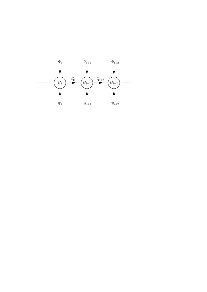
Figure 1: View at the sites $i,i+1$, and $i+2$ of the moose diagram for a deconstructed large extra dimension compactified on $\mathcal{S}^{1}$. Each circle corresponds to one $U(1)_{i}\equiv G_{i}$ gauge group and each arrow pointing towards (outwards) a circle represents a field with negative (positive) charge under this group.

We minimize the potential by going to the real basis

$$Q_{i}=q_{i}^{a}+{\text{i}}q_{i}^{b}\longrightarrow\left(\begin{matrix}q_{i}^{a}\\ q_{i}^{b}\end{matrix}\right),\quad\Phi_{i}=\phi_{i}^{a}+{\text{i}}\phi_{i}^{b}\longrightarrow\left(\begin{matrix}\phi_{i}^{a}\\ \phi_{i}^{b}\end{matrix}\right),$$ (2)

where we are interested in a minimum of $V$ with the following vacuum structure

$$\langle Q_{i}\rangle=\left(\begin{matrix}u\\ 0\end{matrix}\right),\quad\langle\Phi_{i}\rangle=\left(\begin{matrix}v\\ 0\end{matrix}\right),\quad i=1,2,\ldots,N,$$ (3)

i.e., all link variables $Q_{i}$ have a real universal vacuum expectation value (VEV) $u$ and all site variables $\Phi_{i}$ have a real universal VEV $v$. The conditions for an extremum of the potential $V$ are $\partial V/\partial\phi_{i}^{a,b}=\partial V/\partial q_{i}^{a,b}=0$, where the explicit forms are given in the Eqs. (56), (57), (58), and (59) in Appendix A. Requiring $\partial V/\partial\phi_{i}^{a}=0$ leads for the VEVs in Eq. (3) to the minimization condition

$$m^{2}+\left[\lambda_{1}+(N-1)\lambda_{4}\right]v^{2}+(N\lambda_{3}+\frac{1}{2}\lambda_{6})u^{2}+\mu u=0,$$ (4)

where $\langle\partial V/\partial\phi_{i}^{b}\rangle=0$ is automatically fulfilled for these VEVs. Demanding $\partial V/\partial q_{i}^{a}=0$ yields with Eq. (3) the minimization condition

$$u\left[M^{2}+\left(\lambda_{2}+(N-1)\lambda_{5}\right)u^{2}+(N\lambda_{3}+\frac{1}{2}\lambda_{6})v^{2}\right]+\frac{1}{2}\mu v^{2}=0,$$ (5)

and $\langle\partial V/\partial q_{i}^{b}\rangle=0$ is again satisfied for these VEVs. Solving Eq. (4) for $v^{2}$ and substituting $v^{2}$ into Eq. (5), we obtain a cubic equation for $u$, which has the real solution

$$u=\frac{m^{2}\mu}{2\left[\lambda_{1}+(N-1)\lambda_{4}\right]M^{2}}+\mathcal{O}(M^{-4}),$$ (6)

where we have expanded for large $M$. From Eq. (6) we conclude that for large $M\gg v,m$ and moderate $N$, one obtains a naturally small and positive value for $u$, since the VEVs of the link variables are suppressed via the type-II seesaw mechanism [19, 20]. Furthermore, from the Eqs. (4) and (6), one finds

$$v^{2}=\frac{-m^{2}}{\lambda_{1}+(N-1)\lambda_{4}}+\mathcal{O}(M^{-2}).$$ (7)

Choosing the masses of the link fields in the range $M\simeq 10^{8}\ldots 10^{9}\>{\text{GeV}}$, we therefore obtain $v\simeq 10^{2}\>{\text{GeV}}$ and a seesaw suppressed value $u\simeq 10^{-1}\ldots 10^{-3}\>{\text{eV}}$ of the inverse lattice spacing which corresponds to a sub-mm separation of the lattice sites.

Kinetic and mass terms

The mass spectrum of the gauge bosons $A_{i\mu}$ arises via the Higgs mechanism from the kinetic terms of the scalars $\Phi_{i}$ and $Q_{i}$:

$$\mathcal{L}_{\text{kin}}[\Phi_{i},Q_{i}] = \sum_{i=1}^{N}\left[(D_{\mu}\Phi_{i})^{{\dagger}}D^{\mu}\Phi_{i}+(D_{\mu}Q_{i})^{{\dagger}}D^{\mu}Q_{i}\right]$$ (8)

$$= \sum_{i=1}^{N}\left|(\partial_{\mu}+ig_{i}A_{i\mu})\Phi_{i}\right|^{2}+\left|(\partial_{\mu}+ig_{i}A_{i\mu}-ig_{i+1}A_{(i+1)\mu})Q_{i}\right|^{2}.$$

Let us now examine in some more detail how $\mathcal{L}_{\text{kin}}[\Phi_{i},Q_{i}]$ reproduces a 5D $U(1)$ gauge theory compactified on  $\mathcal{S}^{1}$. For this purpose, we denote by $(x^{\mu},y)$ the bulk coordinates and by $A_{5}$ the 5th component of the bulk $U(1)$ gauge group. When the fields $Q_{n}$ are interpreted as the Higgs links

$$Q_{n}=\frac{u}{\sqrt{2}g_{n}}\exp\left(ig_{n}\int_{an}^{a(n+1)}\text{d}y\,A_{5}(x^{\mu},y)\right)=\frac{u}{\sqrt{2}g_{n}}\exp(ig_{n}aA_{n5}),$$ (9)

where $a$ is the spacing between neighboring branes, we observe that $\sum_{i=1}^{N}(D_{\mu}Q_{i})^{{\dagger}}D^{\mu}Q_{i}$ becomes a lattice approximation of the 5D gauge kinetic term

$$\frac{1}{a}\sum_{i=1}^{N}(D_{\mu}Q_{i})^{{\dagger}}D^{\mu}Q_{i}\longrightarrow-\frac{1}{4}\int_{0}^{R}\text{d}y\,(\partial_{\mu}A_{5}-\partial_{5}A_{\mu})^{2},\,\,\,\,R=Na.$$

Actually, in the non-linear sigma model approximation, $Q_{n}$ can be written as

$$Q_{n}=\frac{u}{\sqrt{2}g_{n}}\exp(ig_{n}\pi_{n}(x^{\mu})/u),$$ (10)

where $\pi_{n}(x^{\mu})$ is the Nambu-Goldstone boson field associated with $Q_{n}$. Comparison with Eq. (9) shows that the effective physical degrees of freedom of the non-linear sigma model field in Eq. (10) are completely captured by the gauge boson and (pseudo) Nambu-Goldstone boson sectors. For universal gauge couplings $g_{i}=g$, we obtain from the last line in Eq. (8) the gauge boson mass terms

$$g^{2}\sum_{i=1}^{N}\left[v^{2}A_{i\mu}A_{i}^{\mu}+u^{2}(A_{i\mu}-A_{(i+1)\mu})^{2}\right],$$ (11)

where the VEVs $v=\left\langle\Phi_{i}\right\rangle$ and $u=\left\langle Q_{i}\right\rangle$ have already been inserted. After diagonalization, the mass eigenvalues $M_{n}$ of the gauge bosons read

$$M_{n}^{2}=g^{2}v^{2}+2g^{2}u^{2}\left(1-\cos 2\pi\frac{n}{N}\right),\,\,\,\,n=1,\dots,N.$$ (12)

This spectrum can be interpreted as follows: For $n\ll N$ or $\left|n-N\right|\ll N$ the link fields generate a linear KK spectrum $\sim n/R=ngu/N$ with an overall mass scale $u\sim 10^{-2}\,\text{eV}$. The fields $\Phi_{i}$ provide in addition for the gauge bosons a constant kink mass of the order $v\sim 10^{2}\,\text{GeV}$. In Sec. 3.4, we will show that this comparably large kink mass suppresses the resulting Casimir energy, which would, for bosonic fields, imply a negative cosmological constant.

The Lagrangian $\mathcal{L}_{\text{mass}}[\Psi_{i},Q_{i}]$ contains terms of the type $Q_{i}^{{\dagger}}\overline{\Psi}_{i\text{L}}\Psi_{(i+1)\text{R}}+\text{h.c.}$ which give after SSB fermion masses of order $u$. In our 4D model, a “naive” transverse lattice of the 5D $U(1)$ theory for a bulk fermion is easily accommodated by taking the mass and mixing terms to be

$$\mathcal{L}_{\text{mass}}[\Psi_{i},Q_{i}]=\frac{u}{2}\cdot\sum_{n=1}^{N}\overline{\Psi}_{n\text{L}}\left[\frac{Q_{n}^{{\dagger}}}{u}\Psi_{(n+1)\text{R}}-\frac{Q_{n-1}}{u}\Psi_{(n-1)\text{R}}\right]+\text{h.c.},$$ (13)

which represents the kinetic term of the fermion in the 5th dimension. In the IR, the Lagrangian in Eq. (13) generates identical KK towers for the left- and right-handed states with masses in the sub-eV range. The exact form of the KK mass spectra of the fermions will be calculated in Sec. 4, where the kinetic term will also be modified to cope with the fermion doubling problem, which occurs in the naive treatment of the fermions. As a result of the small inverse lattice spacing $u$, we will show in Sec. 3.2 that the fermionic Casimir energy induces a small positive cosmological constant for small $N$.

It is also possible to interpret the set of scalars $\Phi_{i}$ as one 5D massive scalar on a transverse lattice. The corresponding deconstruction Lagrangian reads

$$\mathcal{L} = \sum_{i=1}^{N}\left[(D_{\mu}\Phi_{i})^{2}+(m^{2}+M_{b}^{2})\left|\Phi_{i}\right|^{2}+\lambda_{1}\left|\Phi_{i}\right|^{4}\right.$$ (14)

$$- \left.M_{b}^{2}\left(\frac{1}{2}\left|\Phi_{i}\right|^{2}+\frac{1}{2}\left|\Phi_{i+1}\right|^{2}-\Phi_{i}\frac{Q_{i}}{u}\Phi_{i+1}^{{\dagger}}+\text{h.c.}\right)\right],$$

where the terms in the last line mimic in the IR the effects of $-\sum_{i=1}^{N}M_{\text{b}}^{2}\left|\Phi_{i}-Q_{i}\Phi_{i+1}/u\right|^{2}\rightarrow\int_{0}^{R}\text{d}y\,(D_{5}\Phi)^{2}$. Here, the scale $M_{\text{b}}$ defines the lattice spacing in the 5th dimension and the $Q_{i}$ are taken as link fields. Choosing $M_{\text{b}}^{2}=\mu u\sim(10^{4}-10^{5}\,\text{eV})^{2}$, we recover similar terms as in the potential $V$ in Eq. (1). The resulting KK mass spectrum corresponds to the one for the gauge bosons in Eq. (12), but with a compactification scale of the order $M_{\text{b}}$ and a constant kink mass $m\sim 10^{2}\,\text{GeV}$. The latter one is large enough to significantly suppress the Casimir effect for the fields $\Phi_{i}$ in a manner similar to the gauge bosons. Note that the terms in $V$ with coefficients $\lambda_{3},\lambda_{5}$, and $\lambda_{6}$ can be neglected with respect to the expression in Eq. (14), since they become $\sim u^{2}v^{2}$. Furthermore, the term with coefficient $\lambda_{4}$ must be forbidden when requiring for the fields $\Phi_{i}$ only “local” interactions. In such a case, Eq. (14) describes very well all scalar interactions in $V$ which involve the fields $\Phi_{i}$. Note again, that (at the renormalizable level) in a supersymmetric case $\lambda_{4}=0$ due to the holomorphy of the superpotential.

Embedding into a disk

So far, we have viewed the fields $\Phi_{i}$ as scalar site variables. The potential $V$, however, possesses a global symmetry which allows to interpret the fields $\Phi_{i}$ also as link variables by gauging the symmetry. In fact, we can embed the latticized 5th dimension into a disk by adding one further $U(1)$ gauge group $U(1)_{0}$ under which all scalars $\Phi_{i}$ $(i=1,\ldots,N)$ carry the same charge $+1$ while the link fields $Q_{i}$ and the fermions $\Psi_{i}$ are all singlets under $U(1)_{0}$. The moose diagram for these symmetries is shown in Fig. 2

Figure 2: Moose diagram obtained from the latticized circle by adding one further gauge group $U(1)_{0}$ to the center. Each scalar $\Phi_{i}$ carries the charge $+1$ under $U(1)_{0}$ and thus connects as a link field the groups $U(1)_{0}$ and $U(1)_{i}$.

where the extra gauge group $U(1)_{0}$ has been placed in the center of a disk whose boundary is the latticized circle discussed above. Obviously, the addition of the $U(1)_{0}$ group has promoted the scalar site variables from the previous model to link fields, since each $\Phi_{i}$ is now charged as $(+1,-1)$ under the product group $U(1)_{0}\times U(1)_{i}$. Topological properties of this lattice geometry have been analyzed in Ref. [25] and its relation to the doublet-triplet splitting problem was addressed in Ref. [26]. It is important to note, that the extra gauge group $U(1)_{0}$ does not affect the scalar potential $V$ and hence the replicated type-II seesaw mechanism which ensures the smallness of the VEVs $u=\left\langle Q_{i}\right\rangle\sim 10^{-2}\,\text{eV}$ remains unaltered. Choosing the gauge coupling of $U(1)_{0}$ to be equal to the other $U(1)_{i}$ gauge couplings $g$, the Lagrangian generating the gauge boson masses can be written as

$$\mathcal{L}[\Phi_{i},Q_{i}]=\sum_{i=1}^{N}\left|\left(\partial_{u}-igA_{0\mu}+igA_{i\mu}\right)\Phi_{i}\right|^{2}+|(\partial_{\mu}+igA_{i\mu}-igA_{(i+1)\mu})Q_{i}|^{2}.$$

In the basis $(A_{0}^{\mu},A_{N}^{\mu},A_{1}^{\mu},A_{2}^{\mu},\ldots,A_{N-1}^{\mu})$, the $(N+1)\times(N+1)$ gauge boson mass matrix $M^{2}$ takes the form

$$M^{2}=g^{2}v^{2}\left(\begin{matrix}N&-1&-1&-1&\cdots\\ -1&1&0&0&\cdots\\ -1&0&1&0&\cdots\\ -1&0&0&1&\cdots\\ \vdots&\vdots&\vdots&\vdots&\ddots\end{matrix}\right)+g^{2}u^{2}\left(\begin{matrix}0&0&0&0&\cdots\\ 0&2&-1&0&\cdots\\ 0&-1&2&-1&\cdots\\ 0&0&-1&2&\cdots\\ \vdots&\vdots&\vdots&\vdots&\ddots\end{matrix}\right),$$

where the bottom-right $N\times N$ submatrix of $M^{2}$ is just the gauge boson mass matrix in Eq. (11). Therefore, the mass eigenstates $\tilde{A}_{n}^{\mu}$ $(n=1,\dots,N)$ of this submatrix have masses $M_{n}$ as in Eq. (12). Hence, $M^{2}$ can be brought to diagonal form in two steps. First, we diagonalize the down-right $N\times N$ submatrix which gives in the basis $(A_{0}^{\mu},\tilde{A}_{N}^{\mu},\tilde{A}_{1}^{\mu},\tilde{A}_{2}^{\mu},\dots,\tilde{A}_{N-1}^{\mu})$ a matrix of the structure

$$M^{2}\rightarrow g^{2}v^{2}\left(\begin{matrix}N&-\sqrt{N}&0&0&\cdots\\ -\sqrt{N}&0&0&0&\cdots\\ 0&0&0&0&\cdots\\ 0&0&0&0&\cdots\\ \vdots&\vdots&\vdots&\vdots&\ddots\end{matrix}\right)+\left(\begin{matrix}0&0&0&0&\cdots\\ 0&M_{N}^{2}&0&0&\cdots\\ 0&0&M_{1}^{2}&0&\cdots\\ 0&0&0&M_{2}^{2}&\cdots\\ \vdots&\vdots&\vdots&\vdots&\ddots\end{matrix}\right).$$

We therefore see, that the rotation in the $N\times N$ sub-space has almost diagonalized the total mass matrix. Next, the diagonalization of $M^{2}$ is completed by a rotation in the $(A_{0}^{\mu},\tilde{A}_{N}^{\mu})$ subspace an angle $\theta=\arctan[\frac{1}{2}(\sqrt{4+(N-1)^{2}/N}-(N-1)/\sqrt{N})]$. From this we observe, that $\tilde{A}_{1}^{\mu},\tilde{A}_{2}^{\mu},\dots,\tilde{A}_{N-1}^{\mu}$ are mass eigenstates of $M^{2}$ since the mixing of these states with $A_{0}^{\mu}$ is zero. In other words, $\tilde{A}_{1}^{\mu},\tilde{A}_{2}^{\mu},\dots,\tilde{A}_{N-1}^{\mu}$ are exactly localized on the boundary of the disk. The remaining two gauge boson mass eigenstates of $M^{2}$ are linear combinations of $A_{0}^{\mu}$ and $\tilde{A}_{N}^{\mu}$ which are parameterized by the mixing angle $\theta$. In configuration space, the wave function profiles of these mass eigenstates read $1/\sqrt{N(N+1)}\cdot(N,-1,-1,\dots,-1)$, which has mass $gv\sqrt{N+1}$, and $1/\sqrt{N+1}\cdot(1,1,\dots,1)$, which is a zero mode. Obviously, the former massive state is primarily composed of $A_{0}^{\mu}$ and becomes arbitrarily well located on the site in the center for $N\gg 1$. Correspondingly, the flat distribution of the zero mode over the disk shows that the admixture of $A_{0}^{\mu}$ to the zero mode vanishes in the limit $N\rightarrow\infty$. Indeed, for large $N$ the mixing angle is approximately $\theta\sim\sqrt{N}/(N-1)$ and the field $A_{0}^{\mu}$ “decouples” from the rest of the gauge bosons such that we effectively recover on the boundary of the disk a deconstructed 5D $U(1)$ gauge theory as above. Note that in $V$, each tri-linear term $\propto\mu\Phi_{i}Q_{i}\Phi_{i+1}^{{\dagger}}$ corresponds in Fig. 2 to a small triangle and is therefore interpreted as a gauge-invariant plaquette term with trivial holonomy in the lowest energy state. The system with real VEVs as in Eq. (3) is gauge-equivalent with a vacuum structure

$$\left\langle Q_{n}\right\rangle=u\cdot e^{i2\pi/N},\,\,\,\,\left\langle\Phi_{n}\right\rangle=v\cdot e^{i2\pi n/N},\,\,\,\,n=1,\dots,N,$$

which maintains an equivalence between the links on the boundary under a rotation of the disk by an angle $2\pi/N$. This rotation yields a representation of the fundamental group of the boundary, which is $Z_{N}$ [26].

3 Casimir Energies and the Cosmological Constant

The Casimir effect is a notable exception from the normal ordering procedure in quantum field theories. It occurs when quantum fields have to obey certain boundary conditions, e.g., the electric component of the photon field, restricted between two parallel conducting plates, has to vanish on the plates. This causes a geometry dependent vacuum energy density inducing a force on the plates. Therefore, the Casimir effect is a macroscopic quantum phenomenon, which is experimentally well established [27]. For a recent review of the effect and its applications see, e.g., Ref. [28].

It has been pointed out, that the Casimir effect is also relevant in higher-dimensional theories [10], where the bulk fields are subject to boundary conditions associated with a non-trivial space-time topology. To establish contact with the discussion in Sec. 2, let us from now on restrict our considerations mainly to the Casimir effect in a 5D $U(1)$ gauge theory compactified on the circle $\mathcal{S}^{1}$ with circumference $R$. After integrating out the extra dimension, the number of KK modes for each bulk field is typically given by $N\sim M_{*}R/2\pi$. In the effective 4D description, each mode contributes, upon quantization, a divergent amount of zero-point energy to the total vacuum energy density, which has the form of a cosmological constant. Even for quantum fields in flat Minkowski space-time, there are always such contributions, which are usually discarded by normal-ordering. These divergent terms arise as VEVs of the Hamiltonian density $\mathcal{H}$, which can be written as an integral over the energy $\omega(p)$ of a field mode with momentum $p$ and mass $M$, i.e., $\left\langle\mathcal{H}\right\rangle\propto\int\text{d}^{3}p\cdot\omega(p)$ with $\omega^{2}=\vec{p}^{\,2}+M^{2}$. In the effective 4D description of the extra-dimensional theory, the total energy density of the $N$ KK field modes can then be brought into the form

$$\rho\propto\sum_{n=1}^{N}\int\text{d}^{3}p\cdot\sqrt{\vec{p}^{\,2}+M^{2}+f(n)},$$

where the function $f(n)$ depends on $N$, $R$, and the spin of the fields. Without any knowledge of the 5th dimension, it would not be clear how to put these UV divergent expressions in a sensible (finite) form. However, since we can interpret the KK tower in terms of an underlying higher-dimensional theory with certain boundary conditions, the 5D Casimir effect provides a well-known procedure to handle these UV divergences in four dimensions. With this, one obtains an unambiguous finite expression for the vacuum energy.

Since the UV divergences are all subtracted in the renormalization program, Casimir energies can be regarded as an IR effect which is insensitive to the UV details of the theory. We hence expect essentially similar Casimir energies to emerge in a class of models which have identical 5D physics as an IR limit but may differ significantly in the UV. In this section, we shall examine this aspect more properly by considering the Casimir effect for a 5D theory which is treated in the UV as a transverse lattice for the extra dimension. In this framework, we will hence be working in a total manifold with topology $\mathcal{M}\times\mathcal{S}_{\text{lat}}^{1}$, where $\mathcal{M}$ is the (continuous) Minkowski space and $\mathcal{S}_{\text{lat}}^{1}$ denotes the latticized 5th dimension compactified on the circle.

In Sec. 3.1, we first discuss the possible field configurations in $\mathcal{M}\times\mathcal{S}^{1}$ before we determine the Casimir energy for a real 5D scalar field $\phi$ and calculate the effective cosmological constant in the transverse lattice. The results for other bosonic fields differ at most by a simple factor, taking into account the degrees of freedom, e.g., one massive vector field counts as $3$ real scalars. Next, in Sec. 3.2, we will perform the analogical calculation for Dirac fermions. Finally, we briefly summarize in Sec. 3.3 our results for massless fields, and in Sec. 3.4 we discuss the effect of a kink mass term.

3.1 The Casimir effect for scalar fields

At the quantum level, global properties of non-trivial space-time topology may be probed by the Casimir effect which is sensitive to the IR structure of a theory. In this context, the existence of inequivalent field configurations associated with the different boundary conditions in the space-time manifold is of special interest. The impact of boundary conditions on the Casimir energies of fields propagating in a non-trivial space-time becomes already evident for the simple example of a 5D theory with topology $\mathcal{M}\times\mathcal{S}^{1}$. For this case, let us now describe the possible field configurations in the language of orbifolds. To this end, we consider a 5D scalar field $\phi$ defined on the simply connected manifold $\mathcal{M}\times\mathbb{R}^{1}$, where the real line $\mathbb{R}^{1}$ is described by the coordinate $y$. We assume that $\mathbb{R}^{1}$ and the field $\phi$ are both subject to a discrete symmetry group $K$. Here, we actually take $K=\mathbb{Z}$, the additive group of integers. The group $K$ acts on $\mathbb{R}^{1}$ as $K:\,y\rightarrow y+m\cdot R$, where $m\in K$ and $R$ is some finite displacement, while the action of $K$ on $\phi$ is $K:\,\phi\rightarrow D(m)\phi$, where $D(m)$ is some (matrix) representation of $K$. Now, one can orbifold the theory by requiring the field $\phi$ to be invariant under both these actions. Then, the equivalence relation $y\sim y+R$ imposed by $K$ on $\mathbb{R}^{1}$ constrains the true physical space to be the smooth manifold $\mathcal{M}\times\mathbb{R}^{1}/\mathbb{Z}=\mathcal{M}\times\mathcal{S}^{1}$, where the circle $\mathcal{S}^{1}$ has the circumference $R$. For the simple case of a real field $\phi$, we can take the matrices $D(m),\,m\in K$ to form a representation of $GL(1,\mathbb{R})\sim O(1,\mathbb{R})$ which is just the group $Z_{2}=\left\{+1,-1\right\}$. As a result, $\phi(y=0)$ and $\phi(y=R)$ are only equal up to a sign, which can also be understood in the context of fibre bundle theory. In this framework [31], the field $\phi$ is interpreted as a cross section of a vector bundle, where the fibre is a real line $\mathbb{R}$. Then we have two possibilities to attach the fibre on the base space $\mathcal{M}\times\mathcal{S}^{1}$. The first one corresponds to forming a product bundle of the base space and the real line, implying a cylinder-like structure and thus periodic boundary conditions for the field, $\phi(y+R)=\phi(y)$. On the other hand, one can form a non-product bundle by twisting the fibres which yields a Möbius band and therefore, $\phi$, as a cross section, obeys anti-periodic boundary conditions

$$\phi(y+mR)=(-1)^{m}\phi(y),\,\,\,\,m\in\mathbb{Z},$$

because one must cycle twice through the circle $\mathcal{S}^{1}$ to completely traverse the Möbius band. In the latter case, the field $\phi$ is called a twisted field, whereas cross sections through the product bundle are untwisted fields. Locally, both bundle types have the same product structure, but globally they differ significantly. These two bundles are the only ones that can be formed by gluing together two trivial real vector bundles. They represent the two possibilities of matching the vector bundles by transition functions, which are the elements of the structure group, in our case $Z_{2}$, that acts on the fibre $\mathbb{R}^{1}$. Since untwisted and twisted bundles provide inequivalent cross sections, they yield inequivalent degrees of freedom of the field $\phi$, which must be considered in the Casimir effect.

Turning to the calculation of Casimir energies, we will first treat the compactified extra dimension to be continuous, before we examine the lattice description. As above, the position in the extra-dimensional space is described by the spatial coordinate $y$ and the corresponding momentum is called $q$. For a real bulk-scalar $\phi$ in the flat manifold $\mathcal{M}\times\mathcal{S}^{1}$, it is sensible to use the plane wave Ansatz

$$\phi(t,\vec{x},y)=A\cdot\exp(i\omega t-i\vec{p}\vec{x}-iqy),$$ (15)

where $A$ is a normalization factor. As discussed previously, the untwisted field configuration is fixed by periodic boundary conditions,

$$\phi(y+R)=\phi(y)\,\,\,\,\Longrightarrow\,\,\,\,e^{-iqR}=1,$$

implying a discrete momentum spectrum:

$$q=2\pi\frac{n}{R},\,\,\,\,n\in\mathbb{Z}.$$ (16)

For twisted fields we use anti-periodic boundary conditions

$$\phi(y+mR)=(-1)^{m}\phi(y),\,\,\,\,m\in\mathbb{Z}\,\,\,\,\Longrightarrow\,\,\,\,e^{-iqR}=-1,$$

which yield the discrete momentum spectrum

$$q=2\pi\frac{(n-\frac{1}{2})}{R},\,\,\,\,n\in\mathbb{Z}.$$ (17)

Since this is the only difference which is relevant for the following calculations, we will work with untwisted fields and replace $n$ by $n-1/2$ when needed.

Discretization

Taking the latticized nature of the 5th dimension into account, the discretization of the circle $\mathcal{S}^{1}$ also forces the coordinate $y$ to be discrete. Assuming $N$ lattice sites with a universal lattice spacing $a$, the circumference of the 5th dimension is given by $R=Na$, and the position $y$ of each site can be described by a coordinate index $j$,

$$y=a\cdot j,\,\,\,\,j=1,\dots,N.$$ (18)

From the standard definition for a derivative in the continuum,

$$\frac{\partial\phi}{\partial y}(y)=\lim_{a\rightarrow 0}\frac{\phi(y+a)-\phi(y)}{a},$$

follows the discrete forward and backward difference operators $\partial_{5}\phi$ and $(\partial_{5}\phi)^{{\dagger}}$:

$$\frac{\partial\phi}{\partial y}\longrightarrow(\partial_{5}\phi) := a^{-1}(\phi(j+1)-\phi(j)),$$

$$\left(\frac{\partial\phi}{\partial y}\right)^{{\dagger}}\longrightarrow(\partial_{5}\phi)^{{\dagger}} := a^{-1}(\phi(j)-\phi(j-1)).$$

By inserting the Ansatz (15) for $\phi$ we find

$$\partial_{5}\phi=a^{-1}(e^{-iqa}-1)\phi,\,\,\,\,(\partial_{5}\phi)^{{\dagger}}=a^{-1}(1-e^{iqa})\phi,$$

and

$$\partial_{5}^{{\dagger}}\partial_{5}\phi=-2a^{-2}(1-\cos qa)\phi.$$

The Klein-Gordon equation for a real 5D scalar field $\phi$ with mass $M_{\text{s}}$ reads

$$\left[\frac{\partial^{2}}{\partial t^{2}}-\nabla^{2}-\partial_{5}^{{\dagger}}\partial_{5}+M_{\text{s}}^{2}\right]\phi=0,$$

and determines the energy $\omega$ of a field mode with the momenta $\vec{p}$ and $q$:

$$\omega^{2}=\vec{p}^{\,2}+m^{2},\,\,\,\,m^{2}:=2a^{-2}(1-\cos qa)+M_{\text{s}}^{2}.$$

The 5D energy-momentum tensor of the real scalar field $\phi$ has the form

$$T_{AB}=(\phi_{,A})^{{\dagger}}(\phi_{,B})-\frac{1}{2}g_{AB}g^{CD}(\phi_{,C})^{{\dagger}}(\phi_{,D})+\frac{1}{2}g_{AB}M_{\text{s}}^{2}\phi^{{\dagger}}\phi,$$ (19)

where $A,B,C,\dots$ are 5D coordinate indices. Here, $A=0$ is the time-like index, $A=1,2,3$ are spatial indices, corresponding to the uncompactified $3$-space, and $A=5$ characterizes the extra spatial dimension. The 5D energy density $\rho_{5}$ is the $00$-component of $T_{AB}$:

$$\rho_{5}=T_{00}=\frac{1}{2}(\partial_{0}\phi)^{{\dagger}}(\partial_{0}\phi)+\frac{1}{2}(\nabla\phi)^{{\dagger}}(\nabla\phi)+\frac{1}{2}(\partial_{5}\phi)^{{\dagger}}(\partial_{5}\phi)+\frac{1}{2}M_{\text{s}}^{2}\phi^{{\dagger}}\phi.$$ (20)

By averaging over all directions of the isotropic $3$-space, we obtain the pressure $p_{5}$ of the scalar field $\phi$:

$$p_{5}=\frac{1}{3}\sum_{i=1}^{3}T_{ii}=\frac{1}{3}\left[(\nabla\phi)^{{\dagger}}(\nabla\phi)+\frac{1}{2}(\partial_{0}\phi)^{{\dagger}}(\partial_{0}\phi)-\frac{1}{2}(\nabla\phi)^{{\dagger}}(\nabla\phi)-\frac{1}{2}(\partial_{5}\phi)^{{\dagger}}(\partial_{5}\phi)-\frac{1}{2}M_{\text{s}}^{2}\phi^{{\dagger}}\phi\right].$$ (21)

The (canonical) quantization of the field $\phi$ leads to the field operator

$$\hat{\phi}(t,\vec{x},y)=\sqrt{V_{3}}\int\text{d}^{3}p\sum_{n=1}^{N}\left(\phi(\vec{p},n)a_{\vec{p},n}+\phi^{{\dagger}}(\vec{p},n)a_{\vec{p},n}^{{\dagger}}\right),$$ (22)

where $a_{p,n}$ and $a_{p,n}^{{\dagger}}$ obey the bosonic commutator relations

$$[a_{\vec{p},n},a_{\vec{p}^{\,\prime},n^{\prime}}^{{\dagger}}]=V_{3}^{-1}\delta(\vec{p}-\vec{p}^{\,\prime})\delta_{nn^{\prime}}\,,\,\,\,\,[a,a]=[a^{{\dagger}},a^{{\dagger}}]=0.$$

The energy-momentum operator $\hat{T}_{AB}$ is obtained by replacing $\phi$ in Eq. (19) by the field operator $\hat{\phi}$. After some calculation (see Appendix B), we arrive at the energy density $\rho_{5}$ and the pressure $p_{5}$ of the 5D quantized field $\phi$,

$$\rho_{5}=\left\langle 0\right|\hat{T}_{00}\left|0\right\rangle = \frac{1}{2(2\pi)^{3}R}\int\text{d}^{3}p\sum_{n=1}^{N}\,\omega,$$ (23)

$$p_{5}=\frac{1}{3}\sum_{i=1}^{3}\left\langle 0\right|\hat{T}_{ii}\left|0\right\rangle = \frac{1}{2(2\pi)^{3}R}\int\text{d}^{3}p\sum_{n=1}^{N}\,\frac{\vec{p}^{\,2}}{3\omega}.$$ (24)

Regularization

The momentum integral $\int\text{d}^{3}p=4\pi\int_{0}^{\infty}\text{d}p\cdot p^{2}$ in Eqs. (23) and (24) and thus $\rho_{5}$ and $p_{5}$ are divergent. We introduce therefore a regularization to obtain meaningful, finite expressions. Consider first Eq. (23). Introducing an exponential suppression factor $e^{-(dp)^{2}}$ as regulator function for $d>0$, we have

$$\int\text{d}p\cdot p^{2}\omega \longrightarrow \int_{0}^{\infty}\text{d}p\cdot p^{2}\omega e^{-(dp)^{2}}$$ (25)

$$= \frac{1}{4}m^{2}d^{-2}e^{\frac{1}{2}(dm)^{2}}K_{1}\left({\textstyle\frac{1}{2}}d^{2}m^{2}\right)$$

$$= \frac{1}{2}d^{-4}+\frac{1}{4}m^{2}d^{-2}+\frac{1}{8}m^{4}\left(\frac{1}{4}+\frac{1}{2}\gamma-\ln 2+\ln(dm)\right)+\mathcal{O}(d^{6}m^{6}),$$

where $K_{n}(x)$ is the modified Bessel function of the second kind of the order $n$ and $\gamma=0,577\dots$ is the Euler-Mascheroni constant. The limit $d\rightarrow 0$ removes the regulator and recovers the divergence. Before taking that limit, a renormalization has to be carried out to remove the potentially divergent terms. Alternatively to the exponential regulator function in Eq. (25), one can also apply dimensional regularization by moving to $n$ space-time dimensions. To be specific,

$$\int\text{d}^{3}p\cdot\omega \longrightarrow \mu^{(4-n)}S(n-1)\cdot\int_{0}^{\infty}\text{d}p\cdot p^{(n-2)}\cdot\omega$$

$$= -\frac{1}{2}m^{4}\left(\frac{\mu}{m}\right)^{(4-n)}\pi^{(n/2-1)}\Gamma\left(-\frac{n}{2}\right)$$

$$\stackrel{{\scriptstyle n\rightarrow 4}}{{=}} (4\pi)\frac{1}{8}m^{4}\left[(n-4)^{-1}+\frac{1}{2}\gamma+\ln\left(\frac{m}{\mu}\right)+\mathcal{O}(n-4)\right]_{n\rightarrow 4},$$

where the arbitrary energy scale $\mu$ has been introduced to keep the dimension of the whole term constant, and $S(n)$ is the surface area of an $n$-ball.

For a curved background space-time [32], one would decompose $\rho$ into a divergent and a finite term, so that the former one has the form of a cosmological term in Einsteins´s equations. Then the divergences would be absorbed into renormalized coupling constants (like $\Lambda$), and the finite remainder is called the renormalized energy density or, in our case, the Casimir energy density. Here, such a general treatment is not necessary because the divergence also arises in flat space-time, like our $\mathcal{M}\times\mathcal{S}^{1}$-manifold, but there are neither cosmological terms nor Einstein´s equations. In order to get rid of the divergence, one simply subtracts the corresponding part of the energy density of the same field in a Minkowski-like space-time with the same dimensions, i.e., $\mathcal{M}\times\mathbb{R}^{1}$ in our case. This kind of renormalization works because the 5D Minkowski space suffers from the same divergence as the $\mathcal{M}\times\mathcal{S}^{1}$ space-time but exhibits no Casimir effect.

Before discussing the details of the renormalization process, we determine the regularized form of the pressure $p$ of the 5D quantized field $\phi$. The regularization with the exponential suppression factor with $d>0$ goes along the same lines as above:

$$\int\text{d}p\cdot p^{2}\frac{p^{2}}{\omega} \longrightarrow \int_{0}^{\infty}\text{d}p\cdot p^{2}\frac{p^{2}}{\omega}e^{-(dp)^{2}}$$ (26)

$$= \frac{1}{4}m^{2}d^{-2}e^{\frac{1}{2}(dm)^{2}}\left(d^{2}m^{2}K_{0}\left({\textstyle\frac{1}{2}}d^{2}m^{2}\right)+(1-d^{2}m^{2})K_{1}\left({\textstyle\frac{1}{2}}d^{2}m^{2}\right)\right)$$

$$= \frac{1}{2}d^{-4}-\frac{1}{4}m^{2}d^{-2}-\frac{3}{8}m^{4}\left(\frac{7}{12}+\frac{\gamma}{2}-\ln 2+\ln(dm)\right)+\mathcal{O}(d^{6}m^{6}).$$

Notice that when keeping in in Eqs. (25) and (26) only terms proportional to $m^{4}\ln m$, we obtain an equation of state $p=-\rho$ of a cosmological constant. As we will see next, the calculation of the Casimir effect on the lattice indeed involves for $d\rightarrow 0$ an exact elimination of all terms which are different from $m^{4}\ln m$ thus leaving a finite contribution to the cosmological constant.

Renormalization

The discrete mode sums for the energy density and pressure in Eqs. (23) and (24) are a result of imposing the periodic or anti-periodic boundary conditions on the lattice scalar. For a quantized scalar field $\hat{\phi}$ which lives on the lattice in the same volume of space (with length $R$ in the fifth dimension) and which does not obey such boundary conditions, the energy density and pressure can be written as

$$\rho_{5} = \frac{1}{2(2\pi)^{3}R}\int\text{d}^{3}p\cdot R\int_{0}^{2\pi/a}\frac{\text{d}q}{2\pi}\omega=\frac{1}{2(2\pi)^{3}R}\int\text{d}^{3}p\cdot N\int_{0}^{1}\text{d}s\cdot\omega,$$ (27)

$$p_{5} = \frac{1}{2(2\pi)^{3}R}\int\text{d}^{3}p\cdot R\int_{0}^{2\pi/a}\frac{\text{d}q}{2\pi}\frac{\vec{p}^{\,2}}{3\omega}=\frac{1}{2(2\pi)^{3}R}\int\text{d}^{3}p\cdot N\int_{0}^{1}\text{d}s\frac{\vec{p}^{\,2}}{3\omega},$$ (28)

where $\omega^{2}=\vec{p}^{\,2}+2a^{-2}(1-\cos qa)+M_{\text{s}}^{2}$. In Appendix C, it is explicitly shown how these mode integrals correspond to the uncompactified latticized space. To calculate the Casimir energy density in $\mathcal{M}\times\mathcal{S}_{\text{lat}}^{1}$, we subtract from the energy density (23) of the field subject to the boundary conditions the corresponding energy density (27) of the field without boundary conditions, which gives the renormalized energy density

$$\rho_{5} = \frac{1}{2(2\pi)^{3}R}\int\text{d}^{3}p\left[\sum_{n=1}^{N}\omega-N\int_{0}^{1}\text{d}s\omega\right]$$ (29)

$$= \frac{1}{2(2\pi)^{3}R}\cdot\frac{4\pi}{8}\left[\sum_{n=1}^{N}m^{4}\ln m-N\cdot\int_{0}^{1}\text{d}s\cdot m^{4}\ln m\right]$$

$$= +R^{-5}S_{1}(N),\,\,\,\,\text{(untwisted)}$$

where $m^{2}=2a^{-2}(1-\cos qa)+M_{\text{s}}^{2}$ and where we have introduced the function

$$S_{1}(N) := \frac{1}{4(2\pi)^{2}}N^{4}\cdot\left[\sum_{n=1}^{N}\left(1-\cos 2\pi\frac{n}{N}+\frac{1}{2}a^{2}M_{\text{s}}^{2}\right)^{2}\ln\left(1-\cos 2\pi\frac{n}{N}+\frac{1}{2}a^{2}M_{\text{s}}^{2}\right)\right.$$ (30)

$$- \left.N\cdot\int_{0}^{1}\text{d}s\cdot\left(1-\cos 2\pi s+\frac{1}{2}a^{2}M_{\text{s}}^{2}\right)^{2}\ln\left(1-\cos 2\pi s+\frac{1}{2}a^{2}M_{\text{s}}^{2}\right)\right].$$

In Eq. (29) we have first regulated the expressions with the exponential regulator method in Eq. (25) before applying the relations as given in Appendix C to exactly subtract for $d\rightarrow 0$ all terms of the type

$$\frac{1}{2}d^{-4}+\frac{1}{4}m^{2}d^{-2}+\frac{1}{8}m^{4}\left(\frac{1}{4}+\frac{1}{2}\gamma-\ln 2+\ln(d)\right)+\mathcal{O}(d^{6}m^{6}).$$

For the renormalized pressure of the quantized field, we apply the corresponding subtraction as in Eq. (29), i.e.,

$$p_{5} = \frac{1}{2(2\pi)^{3}R}\int\text{d}^{3}p\left[\sum_{n=1}^{N}\frac{\vec{p}^{\,2}}{3\omega}-N\int_{0}^{1}\text{d}s\frac{\vec{p}^{\,2}}{3\omega}\right]$$ (31)

$$= \frac{-1}{2(2\pi)^{3}R}\cdot\frac{4\pi}{8}\left[\sum_{n=1}^{N}m^{4}\ln m-N\cdot\int_{0}^{1}\text{d}s\cdot m^{4}\ln m\right]$$

$$= -R^{-5}S_{1}(N),\,\,\,\,\text{(untwisted)}$$

where we again regulated the divergent expressions following Eq. (26) and then exactly subtracted for $d\rightarrow 0$ all terms of the form

$$\frac{1}{2}d^{-4}-\frac{1}{4}m^{2}d^{-2}-\frac{3}{8}m^{4}\left(\frac{7}{12}+\frac{1}{2}\gamma-\ln 2+\ln(d)\right)+\mathcal{O}(d^{6}m^{6}).$$

Comparision of Eqs. (29) and (31) shows that the renormalized finite values of $\rho_{5}$ and $p_{5}$ obey an equation of state $p=-\rho$ which is that of a cosmological constant and hence, the renormalization precedure carried out here actually amounts to a renormalization of the effective cosmological constant in the 4D subspace. As a matter of fact, it is sufficient to restrict in the following our considerations to the vacuum energy density alone with corresponding statements for the pressure implied.

In the limit $N\rightarrow\infty$ and $M_{\text{s}}=0$, the function $S_{1}(N)$ converges to the value of a continuous 5th dimension:

$$\lim_{N\rightarrow\infty}S_{1}(N)=-\frac{1}{4(2\pi)^{2}}3\zeta(5)\cdot 4.$$

By integrating out the 5th dimension, we obtain the 4D energy density

$$\rho_{4}=\int_{0}^{R}\text{d}r\cdot\rho_{5}=R\cdot\rho_{5}=-\frac{3\zeta(5)}{(2\pi)^{2}R^{4}}=\frac{1}{R^{4}}\cdot(-0,0787970\dots).\,\,\,\,(\text{untwisted})$$ (32)

In the case of a twisted scalar field everything is like above, but the energy density reads $\rho_{5}=+R^{-5}S_{2}(N)$, where $S_{2}(N)$ is the function $S_{1}(N)$ with $n$ replaced by $n-\frac{1}{2}$. For massless fields ($M_{\text{s}}=0$) we obtain in the continuum limit

$$\lim_{N\rightarrow\infty}S_{2}(N)=+\frac{1}{4(2\pi)^{2}}3\zeta(5)\cdot(4-{\textstyle\frac{1}{4}}),$$

and after integrating out the 5th dimension the 4D energy density reads

$$\rho_{4}=R\cdot\rho_{5}=+\frac{15}{16}\cdot\frac{3\zeta(5)}{(2\pi)^{2}R^{4}}=\frac{1}{R^{4}}\cdot(+0,0738722\dots).\,\,\,\,(\text{twisted})$$ (33)

Obviously, untwisted and twisted fields provide energy densities $\rho_{4}$ of different sign. Note that the values for $\rho_{4}$ in Eqs. (32) and (33) agree with the results in Refs. [33, 34].

3.2 The Casimir effect for fermions

In analogy with the treatment of scalar fields in Sec. 3.1, we will now calculate the Casimir energy density of Dirac fermions. Therefore, a plane wave Ansatz for Dirac spinor fields $\Psi$ in the $\mathcal{M}\times\mathcal{S}^{1}$ manifold is a convenient choice, too:

$$\Psi=\psi\exp(i\omega t-i\vec{p}\vec{x}-iqy).$$ (34)

The boundary conditions, associated with the compactified $\mathcal{S}^{1}$-dimension, provide the discrete momentum spectra. For twisted and untwisted fields we have $q=2\pi(n-\frac{1}{2})/(aN)$ and $q=2\pi n/(aN)$, respectively. Like in Eq. (18) the coordinate $y$ corresponding to the 5th dimension is discrete, $y=a\cdot j$, where $j=1,\dots,N$, and implies an upper bound for the momentum $q$.

Unlike the Klein-Gordon equation for scalars fields, the Dirac equation is linear in the derivatives, and therefore we need a symmetric derivative operator for the discrete $y$-coordinate:

$$\partial_{5}\Psi(j):=\frac{1}{2a}\left(\Psi(j+1)-\Psi(j-1)\right).$$

With the Ansatz (34) we obtain

$$\partial_{5}\Psi(j) = \frac{1}{2a}Nu\cdot\exp(-i\omega t+i\vec{p}\vec{x})\left[\exp(iqa(j+1))-\exp(iqa(j-1))\right]$$

$$= \Psi(j)\cdot\left(+\frac{i}{a}\sin(qa)\right),$$

and together with the 5D Dirac equation for a Dirac field with mass $M_{\text{f}}$,

$$(i\gamma^{A}\partial_{A}-M_{\text{f}})\Psi=0,\,\,\,\,A=0,\dots,3,5,$$

the energy-momentum relation is determined to be

$$\omega^{2}=\vec{p}^{\,2}+m^{2},\,\,\,\,m^{2}:=a^{-2}\sin^{2}qa+M_{\text{f}}^{2}.$$ (35)

The energy-momentum tensor $T_{AB}$ for the Dirac field $\Psi$ has the form

$$T_{AB}=\frac{1}{4}i[\overline{\Psi}\gamma_{A}\partial_{B}\Psi+\overline{\Psi}\gamma_{B}\partial_{A}\Psi-\overline{(\partial_{A}\Psi)}\gamma_{B}\Psi-\overline{(\partial_{B}\Psi)}\gamma_{A}\Psi],$$

and the usual canonical quantization procedure parallels that for scalar fields up to replacing the bosonic commutator relations by the fermionic anti-commutator relations, which give an overall minus sign in the result. The Dirac fermion also has four times the degrees of freedoms of a real scalar, describing particles and anti-particles with two spin states each. In total, the energy density $\rho_{5}$ and pressure $p_{5}$ of a quantized Dirac field differ from the scalar results of Eqs. (23) and (24) only by a factor of $(-4)$ and in the modified energy-momentum relation of Eq. (35), i.e.,

$$\rho_{5} = -\frac{2}{(2\pi)^{3}R}\sum_{n=1}^{N}\int\text{d}^{3}p\cdot\omega,$$ (36)

$$p_{5} = -\frac{2}{(2\pi)^{3}R}\sum_{n=1}^{N}\int\text{d}^{3}p\cdot\frac{\vec{p}^{\,2}}{\omega},$$ (37)

where $\omega^{2}=\vec{p}^{\,2}+a^{-2}\sin^{2}qa+M_{\text{f}}^{2}$. From here on, the regularization and renormalization procedures are identical to the scalar case in Sec. 3.1. This also implies that the equation of state of the fermionic vacuum energy is that of a cosmological constant, $p=-\rho$. Thus, it is sufficient to give the renormalized energy density in five dimensions

$$\rho_{5} = -\frac{2}{(2\pi)^{3}R}4\pi\frac{1}{8}\left[\sum_{n=1}^{N}m^{4}\ln m-N\cdot\int_{0}^{1}\text{d}s\cdot m^{4}\ln m\right]$$

$$= +R^{-5}F_{1}(N),$$

where the function $F_{1}(N)$ in the last equation is defined as

$$F_{1}(N) := -\frac{1}{4(2\pi)^{2}}N^{4}\cdot\left[\sum_{n=1}^{N}\left(\sin^{2}2\pi\frac{n}{N}+a^{2}M_{\text{f}}^{2}\right)^{2}\ln\left(\sin^{2}2\pi\frac{n}{N}+a^{2}M_{\text{f}}^{2}\right)\right.$$ (38)

$$- \left.N\cdot\int_{0}^{1}\text{d}s\cdot\left(\sin^{2}2\pi\frac{n}{N}+a^{2}M_{\text{f}}^{2}\right)^{2}\ln\left(\sin^{2}2\pi\frac{n}{N}+a^{2}M_{\text{f}}^{2}\right)\right],$$

with $R=Na$. For the twisted Dirac field we have

$$\rho_{5}=R^{-5}F_{2}(N),$$

where $F_{2}(N)$ is the function $F_{1}(N)$ with $n$ replaced by $n-\frac{1}{2}$. Unlike the functions $S_{1,2}(N)$ for the scalar fields, the functions $F_{1,2}(N)$ for the fermionic fields have two limit points each, which depend on whether the number of lattice sites $N$ is even or odd. For massless fermions ($M_{\text{f}}=0$) and even $N$ we obtain

$$\lim_{N\rightarrow\infty}F_{1}(N) = -\frac{1}{4(2\pi)^{2}}\cdot 3\zeta(5)\cdot(-32),\,\,\,\,(\text{untwisted})$$

$$\lim_{N\rightarrow\infty}F_{2}(N) = -\frac{1}{4(2\pi)^{2}}\cdot 3\zeta(5)\cdot(+30).\,\,\,\,(\text{twisted})$$

After integrating out the 5th dimension, the 4D Casimir energy densities read

$$\rho_{4} = \frac{32\cdot 3\zeta(5)}{4(2\pi)^{2}R^{4}}=\frac{1}{R^{4}}\cdot(+0,630376\dots),\,\,\,\,(\text{untwisted})$$ (39)

$$\rho_{4} = \frac{-30\cdot 3\zeta(5)}{4(2\pi)^{2}R^{4}}=\frac{1}{R^{4}}\cdot(-0,590978\dots).\,\,\,\,(\text{twisted})$$ (40)

In the case of odd $N$, both functions have the same limit

$$\lim_{N\rightarrow\infty}F_{1}(N)=\lim_{N\rightarrow\infty}F_{2}(N)=\frac{1}{4(2\pi)^{2}}\cdot 3\zeta(5),$$

$$\rho_{4}=\frac{3\zeta(5)}{4(2\pi)^{2}R^{4}}=\frac{1}{R^{4}}\cdot(+0,019699\dots).$$

This behavior seems to be an effect of the lattice (odd-even artefact [23]), since the analytic calculation of Sec. 5 yields the same values as for even $N$. We also notice, that the $N\rightarrow\infty$ limit of the sum of twisted and untwisted results does not depend on whether $N$ is even or odd. Therefore, it is reasonable to consider only this sum as a physical quantity. For finite $N$, this odd-even artefact is illustrated in Fig. 3. Note again, that the results for $\rho_{4}$ in Eqs. (39) and (40) are identical with the values in Ref. [33].

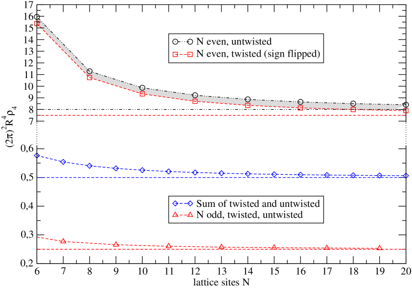
Figure 3: Illustration of the odd-even artefact for fermion fields. The cases of odd and even $N$ are plotted separately, and the circumference $R$ of the 5th dimension is kept constant. For a better representation, we flipped the sign in the results for twisted fields and even $N$. The horizontal lines correspond to the continuum values given in Table 1.

3.3 Summary for massless fields

The calculations of Sec. 3.1 show that the Casimir effect for a real scalar field in the transverse lattice space-time $\mathcal{M}\times\mathcal{S}_{\text{lat}}^{1}$ induces a negative vacuum energy density $\rho$ and therefore a negative effective cosmological constant in the 4D subspace. On the other hand, the fermionic Dirac field of Sec. 3.2 yields a positive contribution to the cosmological constant.

We have already concluded that only the sum of twisted and untwisted fields can be regarded as a physical quantity, and we note that its sign is independent of $N$. Moreover, for a constant circumference $R$ and small $N$, the Casimir energy density $\rho_{4}(N)$ in the transverse lattice setup has already the same order of magnitude as the energy density $\rho_{4}(N\rightarrow\infty)$ in the continuum limit. Specifically, for $N\gtrsim 10$ the continuum result is approximated at the few percent level. Even for a number of lattice sites which is as small as $N=3$, the results differ at most by a factor of $2$, which is clearly shown in Fig. 4.

In the limit $N\rightarrow\infty$ (Table 1), the results for real scalars are the same as in the non-lattice calculation [33, 34], but for the fermions there is an extra factor of $2$ in the energy density of our lattice calculation because of the fermion doubling phenomenon in lattice theory. In a calculation for continuous dimensions, one usually expects, from counting degrees of freedom, that the energy density for Dirac fermions is $(-4)$ times the value of real scalars.

Up to now, we have investigated the Casimir effect for Dirac fermions and real scalars having twisted and untwisted field configurations. When passing to a complex scalar field which transforms under a $U(1)$ gauge group there exist only trivial (untwisted) structures and therefore the charged scalar obeys only periodic boundary conditions. For fermions, on the other hand, the appearance of twisted field modes is related to the double covering map $SL(2,\mathbb{C})\rightarrow SO(3,1)$ which gives rise to inequivalent spin connections [31]. Consequently, even in presence of a simply connected gauge group like $U(1)$ we still have also the anti-periodic boundary condition for the fermions.

$\rho_{4}R^{4}$	untwisted	twisted	sum
real scalar	$-1\cdot(2\pi)^{-2}3\zeta(5)$	$+\frac{15}{16}\cdot(2\pi)^{-2}3\zeta(5)$	$-\frac{1}{16}\cdot(2\pi)^{-2}3\zeta(5)$
fermion, $N$ even	$+8\cdot(2\pi)^{-2}3\zeta(5)$	$-\frac{15}{2}\cdot(2\pi)^{-2}3\zeta(5)$	$+\frac{1}{2}\cdot(2\pi)^{-2}3\zeta(5)$
fermion, $N$ odd	$+\frac{1}{4}\cdot(2\pi)^{-2}3\zeta(5)$	$+\frac{1}{4}\cdot(2\pi)^{-2}3\zeta(5)$	$+\frac{1}{2}\cdot(2\pi)^{-2}3\zeta(5)$

Table 1: The Casimir energy density $\rho_{4}$ multiplied by $R^{4}$ for real massless scalars and Dirac fermions ($M_{\text{s,f}}=0$) in the limit of an infinite number of lattice sites ($N\rightarrow\infty$).

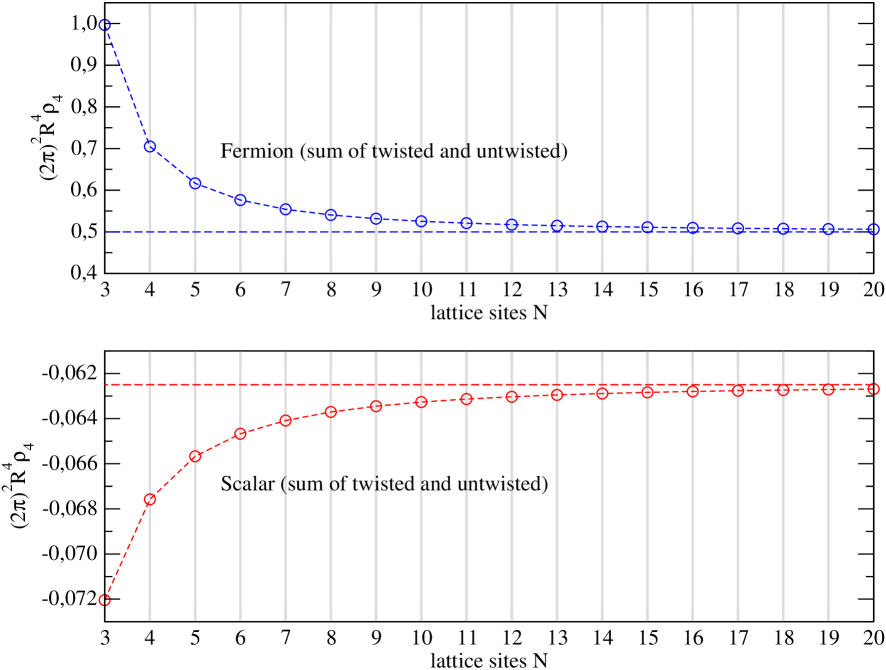
Figure 4: The Casimir energy densities for fermions (upper graph) and real scalars (lower graph). In this plot, $R$ is fixed so that the lattice spacing decreases for increasing $N$. The dashed horizontal lines denote the continuum limit $N\rightarrow\infty$, which has for scalars the value $-\frac{1}{16}$ and for fermions $+\frac{1}{2}$.

3.4 Exponential suppression by a kink mass

So far, we have given results only in the case of vanishing kink mass ($M_{\text{s,f}}=0$). For massive five dimensional fields we observe an approximately exponential suppression of the Casimir energy. This behavior becomes obvious in the analytical calculation for a continuous extra dimension, which is given in Sec. 5. But it is also achieved for the latticized case of Sec. 3, where in the limit of an infinite number of lattice sites ($N\rightarrow\infty$) we approach the values of the analytical formulas (51) and (52). To investigate the suppression behavior depending on the mass $M_{\text{s},\text{f}}$ and the number $N$, we examine the ratio between the energy density of fields with mass $M_{\text{s,f}}$ and that of massless fields. For scalar fields this ratio is defined by

$$\frac{S_{1}(M_{\text{s}}R)+S_{2}(M_{\text{s}}R)}{S_{1}(0)+S_{2}(0)},$$ (41)

where the functions $S_{1,2}(N)$ are taken from Eq. (30) of Sec. 3.1. Analogously, using the functions $F_{1,2}(N)$ from Eq. (38) of Sec. 3.2, the ratio for fermionic fields reads

$$\frac{F_{1}(M_{\text{f}}R)+F_{2}(M_{\text{f}}R)}{F_{1}(0)+F_{2}(0)}.$$ (42)

Both ratios are plotted in Fig. 5 for a range of values of $N$ and $M_{\text{s},\text{f}}R$. The suppression by a kink mass is most minimal for small $N$. In the case of $N=3$ lattice sites, the corresponding ratios are given in Table 2.

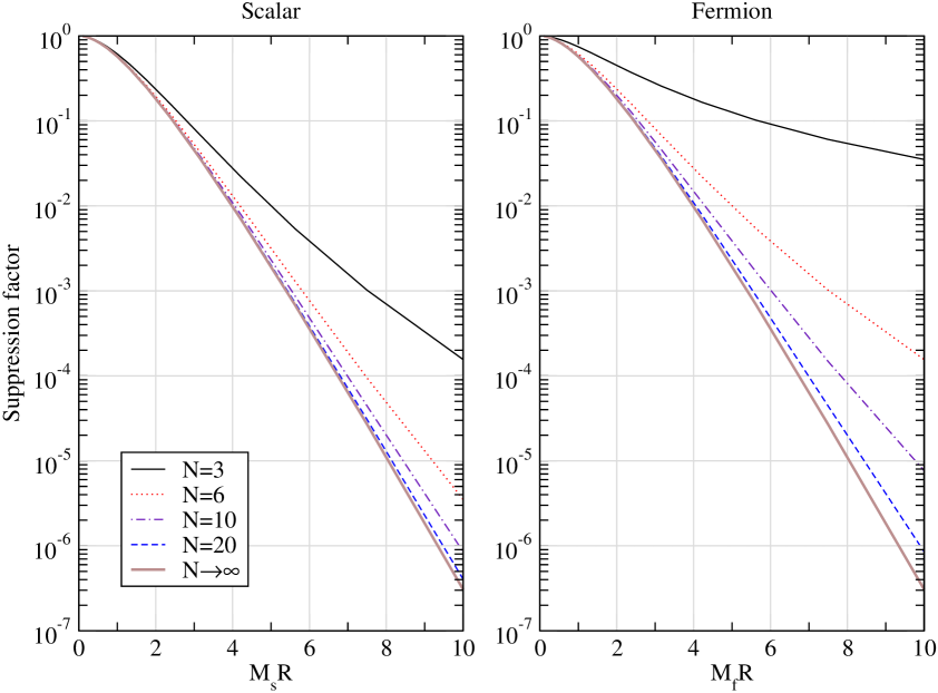
Figure 5: The ratios in Eqs. (41) and (42) of the Casimir energy density between massive and massless fields. The values for $N\rightarrow\infty$ are taken from the analytic formulas in Eqs. (51) and (52).

$M_{\text{s,f}}R$	$1$	$10$	$100$	$1000$	$10^{4}$	$10^{5}$
Scalar	$0,61$	$1,5\cdot 10^{-4}$	$2,9\cdot 10^{-12}$	$3,0\cdot 10^{-20}$	$3,0\cdot 10^{-28}$	$3,0\cdot 10^{-36}$
Fermion	$0,74$	$3,5\cdot 10^{-2}$	$3,7\cdot 10^{-4}$	$3,8\cdot 10^{-6}$	$3,7\cdot 10^{-8}$	$3,7\cdot 10^{-10}$

Table 2: The exponential suppression factors in Eqs. (41) and (42) of the Casimir energy densities for $N=3$ lattice sites, where $M_{\text{s},\text{f}}$ denotes the kink masses of the quantum fields.

field	inverse lattice spacing $a^{-1}$	kink mass $M$	$MR$
scalars $\Phi_{i}$	$M_{\text{b}}\sim 10^{4}-10^{5}\,\text{eV}$	$m\sim 10^{2}\,\text{GeV}$	$N\cdot 10^{6}$
gauge bosons $A_{i}$	$u\sim 10^{-2}\,\text{eV}$	$v\sim 10^{2}\,\text{GeV}$	$N\cdot 10^{13}$
fermions $\Psi_{i}$	$u\sim 10^{-2}\,\text{eV}$	$0$	$0$

Table 3: The fields which can be interpreted as KK modes of a 5D field on a transverse lattice. The kink mass is denoted by $M$, and $R=Na$ is the circumference of $\mathcal{S}_{\text{lat}}^{1}$ with $N$ sites and a lattice spacing $a$. For large values of $MR$ the Casimir effect will be highly suppressed, see Fig. 5 and Table 2.

4 Zero-point Energy in Deconstruction

We will now determine the finite value to the formally infinite vacuum energies of the 4D quantum fields in deconstruction. In the non-linear sigma model approximation, deconstruction yields a transverse lattice description of the $\mathcal{M}\times\mathcal{S}_{\text{lat}}^{1}$ space-time for which we have already calculated the Casimir energies of different fields species in Sec. 3. Then, by correspondence with the parent 5D theory, we are in a position to adopt the renormalization procedure from the Casimir effect of a 5D quantum field to renormalize the divergent vacuum energies of the associated 4D effective KK modes in the deconstruction setup. Specifically, in the model of Sec. 2, all fields, except the fermionic ones, have large kink masses. As a result of Table 3 and Sec. 3.4, the Casimir effect is therefore highly suppressed only for the bosons. Consequently, the fermionic fields $\Psi_{i}$ ($i=1,\dots,N$) provide the dominant part to $\Lambda$, and their total vacuum energy density is given by the sum of zero-point energies

$$\rho=-\frac{2}{(2\pi)^{3}}\sum_{n=1}^{N}\int\text{d}^{3}p\,\omega_{n}(p),$$ (43)

where the $n$th field has a mass $M_{n}$ and momentum modes with energy

$$\omega_{n}(p)=\sqrt{p^{2}+M_{n}^{2}}.$$

We will now show that the masses $M_{n}$ follow exactly the momentum spectrum of the 5D fermion field in Eq. (35), implying that the expression in Eq. (43) becomes identical with the effective unrenormalized Casimir energy density obtained from Eq. (36). This clearly reflects also on a formal level the correspondence between the deconstructed and the 5D theory, by which we can apply the Casimir renormalization techniques of Sec. 3 to the energy density $\rho$ in Eq. (43). To this end, we consider first the kinetic term in Eq. (13). When the link fields $Q_{i}$ acquire universal VEVs $u$ after SSB, $\mathcal{L}_{\text{mass}}[\Psi_{i},Q_{i}]$ takes the form

$$\mathcal{L}_{\text{mass}}[\Psi_{i},Q_{i}]\rightarrow\frac{u}{2}\cdot\sum_{n=1}^{N}\overline{\Psi}_{n\text{L}}\left[\Psi_{(n+1)\text{R}}-\Psi_{(n-1)\text{R}}\right]+\text{h.c.},$$

where $\Psi_{n\text{L,R}}=\frac{1}{2}(1\mp\gamma_{5})\Psi_{n}$ are the left- and right-handed chiral components of the Dirac spinor $\Psi_{n}=(\Psi_{n\text{L}},\Psi_{n\text{R}})^{\text{T}}$. The sum in $\mathcal{L}_{\text{mass}}[\Psi_{i},Q_{i}]$ contains “boundary terms” $-\frac{u}{2}\overline{\Psi}_{1\text{L}}\Psi_{0\text{R}}$ and $\frac{u}{2}\overline{\Psi}_{N\text{L}}\Psi_{(N+1)\text{R}}$, where $\Psi_{0\text{R}}$ and $\Psi_{(N+1)\text{R}}$ are defined by

$$\Psi_{mN+1}=T^{m}\cdot\Psi_{1}\,\,\,\,\text{and}\,\,\,\,\Psi_{0}=T^{m}\cdot\Psi_{mN},\,\,\,\,m\in\mathbb{Z},$$

where we distinguish between untwisted ($T=+1$) and twisted ($T=-1$) fermionic fields. Note that this is the discretized version of the continuum boundary condition

$$\Psi(y+mR)=T^{m}\cdot\Psi(y),\,\,\,\,m\in\mathbb{Z}.$$

Now, the Lagrangian in matrix form reads

$$\mathcal{L}_{\text{mass}}[\Psi_{i}]=\sum_{n,k=1}^{N}\overline{\Psi}_{n\text{L}}M_{nk}\Psi_{k\text{R}}+\text{h.c.},$$

where the mass matrix $M_{nk}$ and its square $M^{2}=MM^{{\dagger}}=M^{{\dagger}}M$ are explicitly given by

$$M=\frac{u}{2}\left[\begin{array}[]{rrrcr}0&+1&&&-T\\ -1&0&+1\\ \\ &\ddots&\ddots&\ddots\\ \\ &&-1&0&+1\\ +T&&&-1&0\end{array}\right],\,\,\,\,M^{2}=\frac{u^{2}}{4}\left[\begin{array}[]{rrrrrrr}2&0&-1&&&-T&0\\ 0&2&0&-1&&&-T\\ -1&0&2&0&-1\\ &\ddots&\ddots&\ddots&\ddots&\ddots\\ &&-1&0&2&0&-1\\ -T&&&-1&0&2&0\\ 0&-T&&&-1&0&2\end{array}\right].$$

The squared masses $m_{n}^{2}$ of the fermions are found to be the eigenvalues of $M^{2}$. Thus, the mass spectrum for untwisted fields reads

$$m_{n}^{2}=u^{2}\sin^{2}2\pi\frac{n}{N},\,\,\,\,n=1,\dots,N,$$

and for the twisted fields we obtain

$$m_{n}^{2}=u^{2}\sin^{2}2\pi\frac{n-\frac{1}{2}}{N},\,\,\,\,n=1,\dots,N,$$

which is consistent with the results in Ref. [23]. Note that only for odd $N$, both spectra become identical, which has already been discussed in the context of the odd-even artefact in Sec. 3.3. With these mass spectra the Casimir energy of the fermions is $(-8)$ times the Casimir energy of a real scalar, whereas in a non-lattice calculation the energies differ only by a factor of $(-4)$ (see Sec. 3.3). This comes again from the well known phenomenon of fermion doubling in lattice theory. One way to remove this problem is to add a Wilson term [37] to $\mathcal{L}_{\text{mass}}[\Psi_{i},Q_{i}]$ in Eq. (13). This then modifies the Lagrangian in Eq. (13):

$$\mathcal{L}_{\text{mass}}=u\cdot\sum_{n=1}^{N}\left[\overline{\Psi}_{n\text{L}}\left(\frac{Q_{n}^{\dagger}}{u}\Psi_{(n+1)\text{R}}-\Psi_{n\text{R}}\right)-\overline{\Psi}_{n\text{R}}\left(\Psi_{n\text{L}}-\frac{Q_{n-1}}{u}\Psi_{(n-1)\text{L}}\right)\right],$$ (44)

which, after SSB, yields the mass matrix $M$. The squared masses $m_{n}^{2}$ of the fermions are now the eigenvalues of $M^{2}$:

$$M=u\cdot\left[\begin{array}[]{rrrrr}-1&+1&&&0\\ &-1&+1\\ &&\ddots&\ddots\\ &&&-1&+1\\ +T&&&&-1\end{array}\right],\,\,\,\,M^{2}=u^{2}\cdot\left[\begin{array}[]{rrrrr}2&-1&&&-T\\ -1&2&-1\\ &\ddots&\ddots&\ddots\\ &&-1&2&-1\\ -T&&&-1&2\end{array}\right],$$

For the untwisted fields we get

$$m_{n}^{2}=2u^{-2}\left(1-\cos 2\pi\frac{n}{N}\right),\,\,\,\,n=1\dots N,$$ (45)

and for the twisted ones $n$ is replaced by $n-\frac{1}{2}$. These mass spectra are identical with the mass spectra of real scalars and yields the usual (continuum) factor $(-4)$ in the vacuum energy density between the two field species. The Wilson term successfully prevented the fermion doubling. Looking at the above mass spectra, we remark that the spectrum (45) for scalars and Wilson-modified fermions does not contain a zero mode in the case of twisted fields.

The Wilson term in Eq. (44) involves explicit Dirac mass terms of the type $u\cdot\overline{\Psi}_{n\text{L}}\Psi_{n\text{R}}$. Let us now examine a possibility to generate such small Dirac masses $u\sim 10^{-2}\,\text{eV}$ in a natural way. For this purpose, we assume two extra SM singlet scalars $Q_{0}$ and $\Phi_{0}$, where $Q_{0}$ has the large mass $M\sim 10^{8}\,\text{GeV}$ and $\Phi_{0}$ has the mass $m\sim 10^{2}\,\text{GeV}$. Also, $Q_{0}$ and $\Phi_{0}$ are singlets under the product group $U(1)^{N}$. Next, we suppose a discrete $Z_{2N}$ symmetry acting on the fields as follows:

$$Z_{2N}: \Phi_{n}\rightarrow e^{i2\pi n/N}\cdot\Phi_{n},\,\,\,\,Q_{n}\rightarrow e^{i2\pi/N}\cdot Q_{n},\,\,\,\,\Psi_{n\text{L}}\rightarrow e^{-i2\pi/N}\cdot\Psi_{n\text{L}},$$

$$\Phi_{0}\rightarrow e^{i\pi/N}\cdot\Phi_{0},\,\,\,\,Q_{0}\rightarrow e^{i2\pi/N}\cdot Q_{0},\,\,\,\,\,\,\,\,n=1,\dots,N$$

All Yukawa interactions of the type $\overline{\Psi}_{n\text{L}}Q_{n}^{{\dagger}}\Psi_{(n+1)\text{R}}/u$ are left unaffected by this symmetry in the Wilson term which forbids all explicit mass terms. The only Yukawa interaction which is, in addition, allowed by the $Z_{2N}$-symmetry is of the form $\overline{\Psi}_{n\text{L}}Q_{0}^{{\dagger}}\Psi_{n\text{R}}$, coupling left- and right-handed states sitting on the same lattice site. Schematically, in presence of the fields $Q_{0}$ and $\Phi_{0}$, the potential in Eq. (1) is modified as follows:

$$V \rightarrow V+m^{2}\Phi_{0}^{{\dagger}}\Phi_{0}+M^{2}Q_{0}^{{\dagger}}Q_{0}+\frac{1}{2}\lambda_{1}(\Phi_{0}^{{\dagger}}\Phi_{0})^{2}+\frac{1}{2}\lambda_{2}(Q_{0}^{{\dagger}}Q_{0})^{2}$$ (46)

$$+(\lambda_{3}Q_{0}^{{\dagger}}Q_{0}+\lambda_{4}\Phi_{0}^{{\dagger}}\Phi_{0})\sum_{j=1}^{N}\Phi_{j}^{{\dagger}}\Phi_{j}+\mu\Phi_{0}^{{\dagger}}Q_{0}\Phi_{0}^{{\dagger}}+\mu^{*}\Phi_{0}Q_{0}^{{\dagger}}\Phi_{0}$$

$$+(\lambda_{3}\Phi_{0}^{{\dagger}}\Phi_{0}+\lambda_{4}Q_{0}^{{\dagger}}Q_{0})\sum_{j=1}^{N}Q_{j}^{{\dagger}}Q_{j},$$

where $\lambda_{1},\dots,\lambda_{4}$ are order unity coefficients. It is thus seen, that the interactions of the scalars $Q_{0}$ and $\Phi_{0}$ also reproduce the structure of $V$ which is relevant for the type-II seesaw mechanism. We therefore expect the mechanism in Sec. 2 for generating sub-mm lattice spacings to be valid (at least qualitatively) also for the modified potential in Eq. (46). From this we find, that the choice $m^{2}<0$ and $M^{2}>0$ leads to VEVs of the orders $\left\langle\Phi_{0}\right\rangle\sim 10^{2}\,\text{GeV}$ and $\left\langle Q_{0}\right\rangle\sim 10^{-2}\,\text{eV}$. We hence conclude, that a small Dirac mass $u$ for the mass terms $u\cdot\overline{\Psi}_{n\text{L}}\Psi_{n\text{R}}$ in Eq. (44) can be generated spontaneously from the Yukawa interaction $\overline{\Psi}_{n\text{L}}Q_{0}^{{\dagger}}\Psi_{nR}$ in a natural way thereby providing an understanding of the mass scales involved in the Wilson term.

The discussion of mass spectra can be easily repeated for the bosonic fields in the model as well. Therefore, we identify the physical vacuum energies of the fields in the model of dimensional deconstruction of Sec. 2 with the finite Casimir results of the calculation in Sec. 3. In Table 3 we give the relevant quantities for the vacuum energy suppression of the fields. Consequently, the Casimir energies of the scalar and vector fields can be neglected due to their large kink masses of order $10^{2}\,\text{GeV}$. In contrast to this, the fermionic fields with KK masses of the order of the small VEV $u\sim 10^{-2}\,\text{eV}$ from Eq. (6) induce a positive contribution to $\Lambda$ which is of the observed order of magnitude already for a small number of $N\lesssim 10$ lattice sites. Finally, it should be noted that we determined only the vacuum energy contributions of quantum fields to $\Lambda$, not its absolute value.

5 The Casimir Effect in the Continuum

In this section, the Casimir effect for a continuous extra dimension will be investigated analytically, where we put special emphasis on the dependence on the mass of the quantum field. In the continuum case, there is no difference in the momentum sums/integrals between fermions and scalars, in both cases the energy function $\omega$ has the form

$$\omega^{2}=\vec{p}^{\,2}+q^{2}+M_{\text{s,f}}^{2},$$

where $q=2\pi n/R$ and $q=2\pi(n+\frac{1}{2})/R$ for untwisted and twisted fields, respectively. We also have to consider negative and unbounded momenta $q$ in the mode sum. So the unrenormalized energy density is

$$\rho\propto\int\text{d}^{3}p\sum_{n=-\infty}^{\infty}\omega.$$

After the regularization used in Eq. (25) of the $\int\text{d}^{3}p$-integral, the remaining sum over the discrete five-momentum $q=2\pi n/R$ can be calculated by using the Abel-Plana formulas [38] as a renormalization prescription:

$$\sum_{n=0}^{\infty}f(n)-\int_{0}^{\infty}\text{d}n\cdot f(n) = \frac{1}{2}f(0)+i\int_{0}^{\infty}\text{d}n\cdot\frac{f(+in)-f(-in)}{\exp(2\pi n)-1},$$ (47)

$$\sum_{n=0}^{\infty}f(n+{\textstyle\frac{1}{2}})-\int_{0}^{\infty}\text{d}n\cdot f(n) = -i\int_{0}^{\infty}\text{d}n\cdot\frac{f(+in)-f(-in)}{\exp(2\pi n)+1}.$$ (48)

The subtraction of the integral on the left hand side corresponds to the subtraction in the first line of Eq. (29). In the case of untwisted fields we have

$$A:=\sum_{n=-\infty}^{\infty}m^{4}(n)\ln[m(n)]-\int_{-\infty}^{\infty}\text{d}n\cdot m^{4}(n)\ln[m(n)],$$

where $m(n)=\sqrt{k^{2}n^{2}+M^{2}}$ and $k:=2\pi/R$, and with the first Abel-Plana formula (47) we rewrite this difference:

$$A=2i\int_{0}^{\infty}\text{d}n\frac{m^{4}(+in)\ln[m(+in)]-m^{4}(-in)\ln[m(-in)]}{\exp(2\pi n)-1}.$$

Assuming $k,n,M\geq 0$, we must consider two cases for the root $m(\pm in)$:

$$\left[k^{2}(\pm in)^{2}+M^{2}\right]^{\frac{1}{2}}=\left\{\begin{array}[]{ll}(M^{2}-k^{2}n^{2})^{\frac{1}{2}}&\,\,\,\text{for}\,\,\,M>kn,\\ \pm i(k^{2}n^{2}-M^{2})^{\frac{1}{2}}&\,\,\,\text{for}\,\,\,M<kn.\end{array}\right.$$

For $a>0$ we can write the logarithm as $\ln(\pm i\cdot a)=\pm i\pi/2+\ln a$, and with $x:=M/k$ we obtain the result

$$A(M)=-2\pi k^{4}\int_{x}^{\infty}\text{d}n\frac{(n^{2}-x^{2})^{2}}{\exp(2\pi n)-1},$$ (49)

which has, in the massless case ($x=0$), the value

$$A=-2\pi k^{4}\frac{3}{4\pi^{5}}\cdot\zeta(5)=-8R^{-4}3\zeta(5).$$

For twisted fields we have to use the second Abel-Plana formula (48). Analogously, we write

$$B(M)=-2i\int_{0}^{\infty}\text{d}n\frac{m^{4}(+in)\ln[m(+in)]-m^{4}(-in)\ln[m(-in)]}{\exp(2\pi n)+1},$$

using $m(n)=\sqrt{k^{2}n^{2}+M^{2}}$, and not $m(n)=\sqrt{k^{2}(n+\frac{1}{2})^{2}+M^{2}}$. Thus, the result becomes

$$B(M)=+2\pi k^{4}\int_{x}^{\infty}\text{d}n\frac{(n^{2}-x^{2})^{2}}{\exp(2\pi n)+1},$$ (50)

where the value for massless fields ($x=0$) is

$$B=+2\pi k^{4}\frac{45}{64\pi^{5}}\cdot\zeta(5)=\frac{15}{2}R^{-4}3\zeta(5).$$

For large masses ($x\gg 1$), approximate expressions for $A(M)$ and $B(M)$ can be given by neglecting the $1$ in the denominator of the Eqs. (49) and (50):

$$\int_{x}^{\infty}\text{d}n\frac{(n^{2}-x^{2})^{2}}{\exp(2\pi n)\pm 1}\stackrel{{\scriptstyle x\gg 1}}{{\sim}}\int_{x}^{\infty}\text{d}n\frac{(n^{2}-x^{2})^{2}}{\exp(2\pi n)}=\frac{4\pi^{2}x^{2}+6\pi x+3}{4\pi^{5}}e^{-2\pi x}.$$

This shows the (approximately) exponential suppression of the Casimir energy by the field mass $M=xk$. Using Eqs. (29) and (49) the effective energy density $\rho_{4}=R\rho$ for untwisted scalar fields is given by

$$\rho_{4} = \frac{1}{8(2\pi)^{2}}\cdot A(M)\,\,\stackrel{{\scriptstyle M=0}}{{=}}\,\,-1\cdot(2\pi)^{-2}R^{-4}3\zeta(5),$$ (51)

and with Eq. (50) we obtain the result for the twisted fields:

$$\rho_{4} = \frac{1}{8(2\pi)^{2}}\cdot B(M)\,\,\stackrel{{\scriptstyle M=0}}{{=}}\,\,+\frac{15}{16}\cdot(2\pi)^{-2}R^{-4}3\zeta(5).$$ (52)

The energy densities for Dirac fermions are just $(-4)$ times the values for the real scalars.

6 Summary and Conclusions

In this paper, we have shown a way how to calculate finite zero-point energies of 4D quantum fields which have a higher-dimensional correspondence in deconstruction. In particular, we constructed a 4D $U(1)^{N}$ model which mimics a latticized large extra dimension with lattice spacings $a$ in the sub-mm range. The vacuum energy of the fermions in our model gives rise to a small and positive contribution $\rho\sim(Na)^{-4}\sim(10^{-3}\,\text{eV})^{4}$ to the cosmological constant in agreement with recent observations. The negative contributions of the scalars and gauge bosons, on the other hand, are exponentially suppressed by large kink masses. Here, we used the correspondence between the 4D zero-point energies and the unrenormalized Casimir energy of 5D quantum fields in a geometric transverse lattice space-time. With inverse lattice spacings in the sub-eV range, our mechanism allows to dynamically generate a large compactified extra dimension with only a small number of lattice sites. This is achieved by giving the link fields a large mass of the order $10^{8}\,\text{GeV}$ and a bulk scalar with kink mass in the electroweak range. Alternatively, this scalar can also be interpreted as a link variable in a space which is topologically a disk. The Casimir effect on the transverse lattice has been investigated for scalar and fermion fields in more detail, thereby taking into account twisted and untwisted field configurations which arise in multiply connected space-times. For the fermions, we observed an odd-even artefact in the Casimir energy which disappears when taking the energy sum of twisted and untwisted fermionic fields. Moreover, due to the naive discretization procedure, we also encountered the effect of fermion doubling, which has been removed by the usual Wilson modification of the fermionic kinetic terms. Furthermore, the suppression of the Casimir effect by a kink mass has been shown for fields on the lattice and in the continuum. Although, this has been utilized only to neglect unwanted contributions to the vacuum energy, it could also be used to generate tiny energy values for quantum fields in small extra dimensions. The combination of methods and mechanisms employed in this work may be generalized for other purposes, and a deeper discussion of vacuum energy in non-trivial topologies poses a task in the future.

Appendix A Minimization of the Potential

We will minimize the scalar potential $V$ in Eq. (1) by going to the real basis in Eq. (2). In this parameterization, the term $\mu\Phi_{i-1}Q_{i}\Phi_{i}^{\dagger}$ in Eq. (1) reads

$$\mu\Phi_{i-1}Q_{i}\Phi_{i}^{\dagger} = \mu\left[\phi_{i-1}^{a}q_{i}^{a}\phi_{i}^{a}-\phi_{i-1}^{b}q_{i}^{b}\phi_{i}^{a}+\phi_{i-1}^{b}q_{i}^{a}\phi_{i}^{b}+\phi_{i-1}^{a}q_{i}^{b}\phi_{i}^{b}\right.$$ (53)

$$\left.+{\text{i}}(\phi_{i-1}^{b}q_{i}^{a}\phi_{i}^{a}+\phi_{i-1}^{a}q_{i}^{b}\phi_{i}^{a}-\phi_{i-1}^{a}q_{i}^{a}\phi_{i}^{b}+\phi_{i-1}^{b}q_{i}^{b}\phi_{i}^{b})\right].$$

Also, the term $\lambda_{6}(Q_{i}Q_{i+1})(\Phi_{i}\Phi_{i+2}^{\dagger})$ in Eq. (1) is given by

$$\lambda_{6}(Q_{i}Q_{i+1})(\Phi_{i}\Phi_{i+2}^{\dagger}) = \lambda_{6}\left[(q_{i}^{a}q_{i+1}^{a}-q_{i}^{b}q_{i+1}^{b})(\phi_{i}^{a}\phi_{i+2}^{a}+\phi_{i}^{b}\phi_{i+2}^{b})\right.$$ (54)

$$\left.-(q_{i}^{b}q_{i+1}^{a}+q_{i}^{a}q_{i+1}^{b})(\phi_{i}^{b}\phi_{i+2}^{a}-\phi_{i}^{a}\phi_{i+2}^{b})\right]$$

$$+{\text{i}}\lambda_{6}\left[(q_{i}^{a}q_{i+1}^{a}-q_{i}^{b}q_{i+1}^{b})(\phi_{i}^{b}\phi_{i+2}^{a}-\phi_{i}^{a}\phi_{i+2}^{b})\right.$$

$$\left.+(q_{i}^{b}q_{i+1}^{a}+q_{i}^{a}q_{i+1}^{b})(\phi_{i}^{a}\phi_{i+2}^{a}+\phi_{i}^{b}\phi_{i+2}^{b})\right].$$

Then, the scalar potential in Eq. (1) can be written as

$$V = \sum_{i=1}^{N}\left\{m^{2}\left[(\phi_{i}^{a})^{2}+(\phi_{i}^{b})^{2}\right]+M^{2}\left[(q_{i}^{a})^{2}+(q_{i}^{b})^{2}\right]+\frac{1}{2}\lambda_{1}\left[(\phi_{i}^{a})^{2}+(\phi_{i}^{b})^{2}\right]^{2}\right.$$

$$+\frac{1}{2}\lambda_{2}\left[(q_{i}^{a})^{2}+(q_{i}^{b})^{2}\right]^{2}+\lambda_{3}\left[(\phi_{i}^{a})^{2}+(\phi_{i}^{b})^{2}\right]\left[\sum_{j=1}^{N}(q_{j}^{a})^{2}+(q_{j}^{b})^{2}\right]$$

$$+\lambda_{4}\left[(\phi_{i}^{a})^{2}+(\phi_{i}^{b})^{2}\right]\left[\sum_{j\neq i}(\phi_{j}^{a})^{2}+(\phi_{j}^{b})^{2}\right]$$

$$+\lambda_{5}\left[(q_{i}^{a})^{2}+(q_{i}^{b})^{2}\right]\left[\sum_{j\neq i}(q_{j}^{a})^{2}+(q_{j}^{b})^{2}\right]$$

$$+\mu\left[\phi_{i-1}^{a}q_{i}^{a}\phi_{i}^{a}-\phi_{i-1}^{b}q_{i}^{b}\phi_{i}^{a}+\phi_{i-1}^{b}q_{i}^{a}\phi_{i}^{b}+\phi_{i-1}^{a}q_{i}^{b}\phi_{i}^{b}\right]$$

$$+\mu\left[\phi_{i}^{a}q_{i+1}^{a}\phi_{i+1}^{a}-\phi_{i}^{b}q_{i+1}^{b}\phi_{i+1}^{a}+\phi_{i}^{b}q_{i+1}^{a}\phi_{i+1}^{b}+\phi_{i}^{a}q_{i+1}^{b}\phi_{i+1}^{b}\right]$$

$$+\frac{1}{2}\lambda_{6}\left[(q_{i-2}^{a}q_{i-1}^{a}-q_{i-2}^{b}q_{i-1}^{b})(\phi_{i-2}^{a}\phi_{i}^{a}+\phi_{i-2}^{b}\phi_{i}^{b})\right.$$

$$\left.-(q_{i-2}^{b}q_{i-1}^{a}+q_{i-2}^{a}q_{i-1}^{b})(\phi_{i-2}^{b}\phi_{i}^{a}-\phi_{i-2}^{a}\phi_{i}^{b})\right]$$

$$+\frac{1}{2}\lambda_{6}\left[(q_{i-1}^{a}q_{i}^{a}-q_{i-1}^{b}q_{i}^{b})(\phi_{i-1}^{a}\phi_{i+1}^{a}+\phi_{i-1}^{b}\phi_{i+1}^{b})\right.$$

$$\left.-(q_{i-1}^{b}q_{i}^{a}+q_{i-1}^{a}q_{i}^{b})(\phi_{i-1}^{b}\phi_{i+1}^{a}-\phi_{i-1}^{a}\phi_{i+1}^{b})\right]$$

$$+\frac{1}{2}\lambda_{6}\left[(q_{i}^{a}q_{i+1}^{a}-q_{i}^{b}q_{i+1}^{b})(\phi_{i}^{a}\phi_{i+2}^{a}+\phi_{i}^{b}\phi_{i+2}^{b})\right.$$

$$\left.-(q_{i}^{b}q_{i+1}^{a}+q_{i}^{a}q_{i+1}^{b})(\phi_{i}^{b}\phi_{i+2}^{a}-\phi_{i}^{a}\phi_{i+2}^{b})\right]$$

$$+\frac{1}{2}\lambda_{6}\left[(q_{i+1}^{a}q_{i+2}^{a}-q_{i+1}^{b}q_{i+2}^{b})(\phi_{i+1}^{a}\phi_{i+3}^{a}+\phi_{i+1}^{b}\phi_{i+3}^{b})\right.$$

$$\left.\left.-(q_{i+1}^{b}q_{i+2}^{a}+q_{i+1}^{a}q_{i+2}^{b})(\phi_{i+1}^{b}\phi_{i+3}^{a}-\phi_{i+1}^{a}\phi_{i+3}^{b})\right]\right\},$$ (55)

where we have symmetrically reorganized the sum, such that all operators carrying the index “$i$” are explicitly displayed. We are interested in a minimum of $V$ with a vacuum structure as given in Eq. (3), i.e., all link variables $Q_{i}$ have a real universal VEV $u$ and all fields $\Phi_{i}$ have a real universal VEV $v$. From Eq. (55) we obtain

$$\frac{\partial V}{\partial\phi_{i}^{a}} = 2m^{2}\phi_{i}^{a}+2\lambda_{1}\left[(\phi_{i}^{a})^{2}+(\phi_{i}^{b})^{2}\right]\phi_{i}^{a}$$ (56)

$$+2\lambda_{3}\phi_{i}^{a}\left[\sum_{j=1}^{N}(q_{j}^{a})^{2}+(q_{j}^{b})^{2}\right]+2\lambda_{4}\phi_{i}^{a}\left[\sum_{j\neq i}(\phi_{j}^{a})^{2}+(\phi_{j}^{b})^{2}\right]$$

$$+\mu[\phi_{i-1}^{a}q_{i}^{a}-\phi_{i-1}^{b}q_{i}^{b}]+\mu\left[q_{i+1}^{a}\phi_{i+1}^{a}+q_{i+1}^{b}\phi_{i+1}^{b}\right]$$

$$+\frac{1}{2}\lambda_{6}\left[(q_{i-2}^{a}q_{i-1}^{a}-q_{i-2}^{b}q_{i-1}^{b})\phi_{i-2}^{a}-(q_{i-2}^{b}q_{i-1}^{a}+q_{i-2}^{a}q_{i-1}^{b})\phi_{i-2}^{b}\right]$$

$$+\frac{1}{2}\lambda_{6}\left[(q_{i}^{a}q_{i+1}^{a}-q_{i}^{b}q_{i+1}^{b})\phi_{i+2}^{a}+(q_{i}^{b}q_{i+1}^{a}+q_{i}^{a}q_{i+1}^{b})\phi_{i+2}^{b}\right],$$

$$\frac{\partial V}{\partial\phi_{i}^{b}} = 2m^{2}\phi_{i}^{b}+2\lambda_{1}\left[(\phi_{i}^{a})^{2}+(\phi_{i}^{b})^{2}\right]\phi_{i}^{b}$$ (57)

$$+2\lambda_{3}\phi_{i}^{b}\left[\sum_{j=1}^{N}(q_{j}^{a})^{2}+(q_{j}^{b})^{2}\right]+2\lambda_{4}\phi_{i}^{b}\left[\sum_{j\neq i}(\phi_{j}^{a})^{2}+(\phi_{j}^{b})^{2}\right]$$

$$+\mu[\phi_{i-1}^{b}q_{i}^{a}+\phi_{i-1}^{a}q_{i}^{b}]+\mu\left[-q_{i+1}^{b}\phi_{i+1}^{a}+q_{i+1}^{a}\phi_{i+1}^{b}\right]$$

$$+\frac{1}{2}\lambda_{6}\left[(q_{i-2}^{a}q_{i-1}^{a}-q_{i-2}^{b}q_{i-1}^{b})\phi_{i-2}^{b}+(q_{i-2}^{b}q_{i-1}^{a}+q_{i-2}^{a}q_{i-1}^{b})\phi_{i-2}^{a}\right]$$

$$+\frac{1}{2}\lambda_{6}\left[(q_{i}^{a}q_{i+1}^{a}-q_{i}^{b}q_{i+1}^{b})\phi_{i+2}^{b}-(q_{i}^{b}q_{i+1}^{a}+q_{i}^{a}q_{i+1}^{b})\phi_{i+2}^{a}\right],$$

which gives for the VEVs in Eq. (3) the minimization condition

$$m^{2}+\left[\lambda_{1}+(N-1)\lambda_{4}\right]v^{2}+(N\lambda_{3}+\frac{1}{2}\lambda_{6})u^{2}+\mu u=0,$$

and $\langle\partial V/\partial\phi_{i}^{b}\rangle=0$ is automatic for these VEVs. The partial derivatives for the link fields $Q_{i}$ are

$$\frac{\partial V}{\partial q_{i}^{a}} = 2M^{2}q_{i}^{a}+2\lambda_{2}\left[(q_{i}^{a})^{2}+(q_{i}^{b})^{2}\right]q_{i}^{a}+2\lambda_{3}q_{i}^{a}\left[\sum_{j=1}^{N}(\phi_{j}^{a})^{2}+(\phi_{j}^{b})^{2}\right]$$ (58)

$$+\mu(\phi_{i-1}^{a}\phi_{i}^{a}+\phi_{i-1}^{b}\phi_{i}^{b})+2\lambda_{5}q_{i}^{a}\left[\sum_{j\neq i}(q_{j}^{a})^{2}+(q_{j}^{b})^{2}\right]$$

$$+\frac{1}{2}\lambda_{6}\left[q_{i-1}^{a}(\phi_{i-1}^{a}\phi_{i+1}^{a}+\phi_{i-1}^{b}\phi_{i+1}^{b})-q_{i-1}^{b}\left(\phi_{i-1}^{b}\phi_{i+1}^{a}-\phi_{i-1}^{a}\phi_{i+1}^{b}\right)\right]$$

$$+\frac{1}{2}\lambda_{6}\left[q_{i+1}^{a}(\phi_{i}^{a}\phi_{i+2}^{a}+\phi_{i}^{b}\phi_{i+2}^{b})-q_{i+1}^{b}\left(\phi_{i}^{b}\phi_{i+2}^{a}-\phi_{i}^{a}\phi_{i+2}^{b}\right)\right],$$

and

$$\frac{\partial V}{\partial q_{i}^{b}} = 2M^{2}q_{i}^{b}+2\lambda_{2}\left[(q_{i}^{a})^{2}+(q_{i}^{b})^{2}\right]q_{i}^{b}+2\lambda_{3}q_{i}^{b}\left[\sum_{j=1}^{N}(\phi_{j}^{a})^{2}+(\phi_{j}^{b})^{2}\right]$$ (59)

$$+\mu(-\phi_{i-1}^{b}\phi_{i}^{a}+\phi_{i-1}^{a}\phi_{i}^{b})+2\lambda_{5}q_{i}^{b}\left[\sum_{j\neq i}(q_{j}^{a})^{2}+(q_{j}^{b})^{2}\right]$$

$$+\frac{1}{2}\lambda_{6}\left[-q_{i-1}^{b}(\phi_{i-1}^{a}\phi_{i+1}^{a}+\phi_{i-1}^{b}\phi_{i+1}^{b})-q_{i-1}^{a}\left(\phi_{i-1}^{b}\phi_{i+1}^{a}-\phi_{i-1}^{a}\phi_{i+1}^{b}\right)\right]$$

$$+\frac{1}{2}\lambda_{6}\left[-q_{i+1}^{b}(\phi_{i}^{a}\phi_{i+2}^{a}+\phi_{i}^{b}\phi_{i+2}^{b})-q_{i+1}^{a}\left(\phi_{i}^{b}\phi_{i+2}^{a}-\phi_{i}^{a}\phi_{i+2}^{b}\right)\right],$$

which leads for the VEVs in Eq. (3) to the minimization condition

$$u\left[M^{2}+\left(\lambda_{2}+(N-1)\lambda_{5}\right)u^{2}+(N\lambda_{3}+\frac{1}{2}\lambda_{6})v^{2}\right]+\frac{1}{2}\mu v^{2}=0,$$

and $\langle\partial V/\partial q_{i}^{b}\rangle=0$ is again satisfied for these VEVs.

Appendix B Energy density and pressure of the quantized scalar field

In Sec. 3.1, we have introduced a real 5D bulk-scalar $\phi$ propagating in a $\mathcal{M}\times\mathcal{S}_{\text{lat}}^{1}$ manifold. To normalize the field modes in Eq. (15), we define the following scalar product for two modes $\phi_{1,2}(\vec{p},n)$ by

$$(\phi_{1},\phi_{2}):=i\int d^{3}x\,a\sum_{j=1}^{N}\,\left(\phi_{1}^{{\dagger}}(\partial_{t}\phi_{2})-(\partial_{t}\phi_{1})^{{\dagger}}\phi_{2}\right),$$

so that the normalization factor $A$ can be fixed by demanding the orthonormality relation

$$\left(\phi(\vec{p},n),\phi(\vec{p}^{\,\prime},n^{\prime})\right)=-V_{3}^{-1}\delta^{(3)}(\vec{p}-\vec{p}^{\,\prime})\delta_{nn^{\prime}},$$

where $V_{3}$ is an arbitrary $3$-volume factor, which leaves the scalar product dimensionless. With the Ansatz in Eq. (15), we find

$$A^{{\dagger}}A=\frac{1}{2\omega(2\pi)^{3}V_{3}R},$$ (60)

where we have applied the relations

$$\int d^{3}x\cdot\exp(i\vec{x}(\vec{p}-\vec{p}^{\,\prime}))=(2\pi)^{3}\delta^{(3)}(\vec{p}-\vec{p}^{\,\prime})\,\,\,\,\text{and}\,\,\,\,\sum_{j=1}^{N}\exp\left(2\pi i\frac{n-n^{\prime}}{N}j\right)=N\delta_{nn^{\prime}}.$$

Now, the $00$-component $\hat{T}_{00}$ and the averaged $ii$-components $\frac{1}{3}\sum_{i=1}^{3}\hat{T}_{ii}$ of the energy-momentum operator $\hat{T}_{AB}$ follow from substituting the field operator $\hat{\phi}$ in Eq. (22) into Eqs. (20) and (21). Here, it is useful to consider the relations

$$(\partial_{0}\hat{\phi})^{{\dagger}}(\partial_{0}\hat{\phi}) = V_{3}^{2}\int d^{3}p\int d^{3}p^{\prime}\sum_{n,n^{\prime}=1}^{N}\left[\partial_{0}\phi(\vec{p},n)a_{\vec{p},n}\cdot\partial_{0}\phi(\vec{p}^{\,\prime},n^{\prime})^{{\dagger}}a_{\vec{p}^{\,\prime},n^{\prime}}^{{\dagger}}+\cdots\right]$$

$$= V_{3}\int d^{3}p\sum_{n=1}^{N}\,A^{{\dagger}}A\cdot\omega^{2}+\cdots$$

$$(\partial_{b}\hat{\phi})^{{\dagger}}(\partial_{b}\hat{\phi}) = V_{3}\int d^{3}p\sum_{n=1}^{N}\,A^{{\dagger}}A\cdot p_{b}^{2}+\cdots\,\,\,\,\forall\,b=1,2,3$$

$$(\partial_{5}\hat{\phi})^{{\dagger}}(\partial_{5}\hat{\phi}) = V_{3}\int d^{3}p\sum_{n=1}^{N}\,A^{{\dagger}}A\cdot 2a^{-2}(1-\cos qa)+\cdots,$$ (61)

where the ellipses ($\cdots$) denote the terms which vanish in the VEVs $\left\langle 0\right|\hat{T}_{AB}\left|0\right\rangle$ due to $\left\langle 0\right|a^{{\dagger}}=a\left|0\right\rangle=0$. When we insert the terms in Eqs. (61) into Eqs. (20) and (21), one obtains, after taking the VEVs of $\hat{T}_{00}$ and $\hat{T}_{ii}$, the energy density $\rho_{5}$ and the pressure $p_{5}$ of the quantized field $\phi$,

$$\rho_{5}=\left\langle 0\right|\hat{T}_{00}\left|0\right\rangle = V_{3}\int\text{d}^{3}p\sum_{n=1}^{N}\,A^{{\dagger}}A\cdot\left[\frac{1}{2}\omega^{2}+\frac{1}{2}\vec{p}^{\,2}+\frac{1}{2}\cdot 2a^{-2}(1-\cos qa)+\frac{1}{2}M_{\text{s}}^{\text{2}}\right]$$

$$= V_{3}\int\text{d}^{3}p\sum_{n=1}^{N}\,A^{{\dagger}}A\cdot\omega^{2},$$

$$p_{5}=\frac{1}{3}\sum_{i=1}^{3}\left\langle 0\right|\hat{T}_{ii}\left|0\right\rangle = V_{3}\int\text{d}^{3}p\sum_{n=1}^{N}\,A^{{\dagger}}A\cdot\left[\frac{1}{3}\vec{p}^{\,2}+\frac{1}{2}\omega^{2}-\frac{1}{2}\vec{p}^{\,2}-\frac{1}{2}2a^{-2}(1-\cos qa)-\frac{1}{2}M_{\text{s}}^{2}\right]$$

$$= V_{3}\int\text{d}^{3}p\sum_{n=1}^{N}\,A^{{\dagger}}A\cdot\frac{\vec{p}^{\,2}}{3\omega},$$

where we have used the energy-momentum relation $\omega^{2}=\vec{p}^{\,2}+2a^{-2}(1-\cos qa)+M_{\text{s}}^{2}$. With the normalization factor $A$ in Eq. (60) we finally arrive at the Eqs. (23) and (24).

Appendix C Renormalization

To gain the finite and unambiguous Casimir energy density, it is necessary to compare the discrete mode sums belonging to the momenta in $\mathcal{S}_{\text{lat}}^{1}$ with the energy density and pressure of a field in a space-time with a non-compactified extra dimension. Regarding Eqs. (23) and (25), the mode sum with respect to the 5th momentum coordinate $q=2\pi n/(aN)$ is of the type

$$\sum_{n=1}^{N}f(n/N),$$

where $f(n/N)$ summarizes the terms in the last line of Eq. (25). From this sum, the mode integral corresponding to a non-compactified $\mathbb{R}^{1}$-dimension can be obtained by cutting out a section of length $R$ of an $\mathbb{R}^{1}$-dimension. This means, that we take the limit of an infinite number $M$ of lattice sites, $M\rightarrow\infty$, while keeping the spacing $a$ constant:

$$\left.\frac{R}{Ma}\sum_{n=1}^{M}f\left(\frac{n}{M}\right)\right|_{M\rightarrow\infty}=\frac{R}{a}\left[\sum_{n=1}^{M}\frac{\Delta n}{M}f\left(\frac{n}{M}\right)\right]_{M\rightarrow\infty}\stackrel{{\scriptstyle s:=n/M}}{{=}}N\cdot\int_{0}^{1}\text{d}s\cdot f(s),$$

where $Ma$ becomes the infinite “length” of $\mathbb{R}^{1}$ and $f(s)$ is the same function as in the $\mathcal{S}_{\text{lat}}^{1}$ mode sum. In the last equation, we have substituted $s:=n/M$ and inserted $\Delta n=1$ so that $\text{d}s=\Delta n/M$ for $M\rightarrow\infty$. Both the sum and the integral are finite since the lattice introduces an UV cutoff. Then the renormalization is performed by subtracting the integral from the sum,

$$\sum_{n=1}^{N}f\left(\frac{n}{N}\right)-N\cdot\int_{0}^{1}\text{d}s\cdot f(s)=\sum_{n=1}^{N}m^{4}\ln m-N\cdot\int_{0}^{1}\text{d}s\cdot m^{4}\ln m,$$ (62)

where only $m^{4}\ln m$ survives since all other terms

$$\frac{1}{2}d^{-4}+\frac{1}{4}m^{2}d^{-2}+\frac{1}{8}m^{4}\left(\frac{1}{4}+\frac{1}{2}\gamma-\ln 2+\ln(d)\right)+\mathcal{O}(d^{6}m^{6})$$

of Eq. (25) either vanish when the regularization is removed for $d\rightarrow 0$ or are completely subtracted due to the following identities:

$$\sum_{n=1}^{N}(1-\cos 2\pi{\textstyle\frac{n}{N}}+{\textstyle\frac{1}{2}}a^{2}M_{\text{s}}^{2})=N\cdot\int_{0}^{1}ds\cdot(1-\cos 2\pi s+{\textstyle\frac{1}{2}}a^{2}M_{\text{s}}^{2})=N(1+{\textstyle\frac{1}{2}}a^{2}M_{\text{s}}^{2}),$$ (63)

$$\sum_{n=1}^{N}(1-\cos 2\pi{\textstyle\frac{n}{N}}+{\textstyle\frac{1}{2}}a^{2}M_{\text{s}}^{2})^{2}=N\cdot\int_{0}^{1}ds\cdot(1-\cos 2\pi s+{\textstyle\frac{1}{2}}a^{2}M_{\text{s}}^{2})^{2}=N({\textstyle\frac{3}{2}}+a^{2}M_{\text{s}}^{2}+({\textstyle\frac{1}{2}}a^{2}M_{\text{s}}^{2})^{2}).$$ (64)

This is also the case for twisted fields, where $n$ is replaced by $n-\frac{1}{2}$.

References

- [1] T. Kaluza, Sitzungsber. Preuss. Akad. Wiss. Berlin (Math. Phys.) K21 (1921) 966; O. Klein, Z. Phys. 37 (1926) 895.
- [2] See, e.g., E. Cremmer and B. Julia, Phys. Lett. B 80 (1978) 48; J. Sherk and J. Schwarz, Nucl. Phys. B 153 (1979) 61.
- [3] I. Antoniadis, Phys. Lett. B 246 (1990) 377; I. Antoniadis, C. Munoz, and M. Quiros, Nucl. Phys. B 397 (1993) 515, hep-ph/9211309; I. Antoniadis, K. Benakli, and M. Quiros, Phys. Lett. B 331 (1994) 313, hep-ph/9403290; J. Lykken, Phys. Rev. D 54 (1996) 3693, hep-th/9603133; I. Antoniadis, S. Dimopoulos, and G. Dvali, Nucl. Phys. B 516 (1998) 70, hep-ph/9710204; J. Lykken and L. Randall, J. High Energy Phys. 0006 (2000) 014, hep-th/9908076.
- [4] N. Arkani-Hamed, A.G. Cohen, and H. Georgi, Phys. Rev. Lett. 86 (2001) 4757, hep-th/0104005.
- [5] C.T. Hill, S. Pokorski, and J. Wang, Phys. Rev. D64 (2001) 105005, hep-th/0104035.
- [6] M.B. Halpern and W. Siegel, Phys. Rev. D11 (1975) 2967.
- [7] W.A. Bardeen and R.B. Pearson, Phys. Rev. D 14 (1976), 547; W.A. Bardeen, R.B. Pearson, and E. Rabinovici, Phys. Rev. D 21 (1980) 1037.
- [8] H.C. Cheng, C.T. Hill, S. Pokorski, and J. Wang, Phys. Rev. D 64 (2001) 065007, hep-th/0104179; H.C. Cheng, C.T. Hill, and J. Wang, Phys. Rev. D 64 (2001) 095003, hep-ph/0105323; C. Csaki, G.D. Kribs, and J. Terning, Phys. Rev. D 65 (2002) 015004, hep-ph/0107266; H.C. Cheng, K.T. Matchev, and J. Wang, Phys. Lett. B 521 (2001) 308, hep-ph/0107268; A. Falkowski, C. Grojean, and S. Pokorski, Phys. Lett. B 535 (2002) 258, hep-ph/0203033; H. Abe, T. Kobayashi, N. Maru, and K. Yoshioka, Phys. Rev. D 67 (2003) 045019, hep-ph/0205344; T. Gregoire and J.G. Wacker, hep-ph/0207164; L. Randall, Y. Shadmi, and N. Weiner, J. High Energy Phys. 0301 (2003) 055, hep-th/0208120; E. Dudas, A. Falkowski, and S. Pokorski, Phys. Lett. B 568 (2003) 281, hep-th/0303155.
- [9] H.B.G. Casimir, Kon. Ned. Akad. Wetensch. Proc. 51 (1948) 793.
- [10] T. Appelquist and A. Chodos, Phys. Rev. Lett. 50 (1983) 141; T. Appelquist and A. Chodos, Phys. Rev. D 28 (1983) 772.
- [11] A.G. Riess et al., Astron. J. 116 (1998) 1009, astro-ph/9805201; S. Perlmutter et al., Astrophys. J. 517 (1999) 565, astro-ph/9812133; D.N. Spergel et al., astro-ph/0302209.
- [12] K.A. Milton, Grav. Cosmol. 9 (2003) 66, hep-ph/0210170.
- [13] N. Arkani-Hamed, S. Dimopoulos, and G.R. Dvali, Phys. Lett. B 429 (1998) 263, hep-ph/9803315.
- [14] I. Antoniadis, N. Arkani-Hamed, S. Dimopoulos, and G.R. Dvali, Phys. Lett. B 436 (1998) 257, hep-ph/9804398.
- [15] N. Arkani-Hamed, S. Dimopoulos, G.R. Dvali, and J. March-Russell, Phys. Rev. D 65 (2002) 024032, hep-ph/9811448; K.R. Dienes, E. Dudas, and T. Gherghetta, Nucl. Phys. B 557 (1999) 25, hep-ph/9811428.
- [16] E.G. Adelberger, B.R. Heckel, and A.E. Nelson, hep-ph/0307284; C.D. Hoyle, U. Schmidt, B.R. Heckel, E.G. Adelberger, J.H. Gundlach, D.J. Kapner, H.E. Swanson, Phys. Rev. Lett. 86 (2001) 1418, hep-ph/0011014; EÖT-WASH Group, E.G. Adelberger, et al., hep-ex/0202008.
- [17] S. Cullen and M. Perelstein, Phys. Rev. Lett. 83 (1999) 268, hep-ph/9903422; V. Barger, T. Han, C. Kao, and R.J. Zhang, Phys. Lett B 461 (1999) 34, hep-ph/9905474; S. Hannestad and G.G. Raffelt, Phys. Rev. Lett. 87 (2001) 051301, hep-ph/0103201; C. Hanhart, D.R. Philips, S. Reddy, and M.J. Savage, Nucl. Phys. B 595 (2001) 335, nucl-th/0007016; S. Hannestad and G.G. Raffelt, Phys. Rev. D 67 (2003) 125008, hep-ph/0304029.
- [18] S. Weinberg, Rev. Mod. Phys. 61 (1989) 1; P.J. Peebles and B. Ratra, Rev. Mod. Phys. 75 (2003) 599, astro-ph/0207347; T. Padmanabhan, Phys. Rept. 380 (2003) 235, hep-th/0212290.
- [19] R.N. Mohapatra and G. Senjanović, Phys. Rev. Lett. 44 (1980) 912.
- [20] E. Ma and U. Sarkar, Phys. Rev. Lett. 80 (1998) 5716, hep-ph/9802445.
- [21] H. Georgi, Nucl. Phys. B 266 (1986) 274.
- [22] M.R. Douglas and G. Moore, hep-th/9603167.
- [23] C.T. Hill and A.K. Leibovich, Phys. Rev. D 66 (2002) 016006, hep-ph/0205057.
- [24] A. Falkowski, H.P. Nilles, M. Olechowski, and S. Pokorski, Phys. Lett. B 566 (2003) 248, hep-th/0212206.
- [25] N. Arkani-Hamed, A.G. Cohen, and H. Georgi, J. High Energy Phys. 0207 (2002), hep-th/0109082.
- [26] E. Witten, hep-ph/0201018.
- [27] M.J. Sparnaay, Physica 24 (1958) 751.
- [28] M. Bordag, U. Mohideen and V.M. Mostepanenko, Phys. Rept. 353 (2001) 1, quant-ph/0106045.
- [29] N. Kan and K. Shiraishi, gr-qc/0212113.
- [30] A. Hebecker and J. March-Russell, Nucl. Phys. B 625 (2002) 128, hep-ph/0107039.
- [31] C.J. Isham, Proc. R. Soc. Lond. A. 362 (1978) 383; C.J. Isham, Proc. R. Soc. Lond. A. 364 (1978) 591; S.J. Avis and C.J. Isham, Nucl. Phys. B 156 (1979) 441.
- [32] N.D. Birrell and P.C.W. Davies, “Quantum Fields In Curved Space”, Cambridge Univ. Pr. (1982).
- [33] P. Candelas and S. Weinberg, Nucl. Phys. B 237 (1984) 397.
- [34] R. Kantowski and K.A. Milton, Phys. Rev. D 36 (1987) 3712.
- [35] A. Pilaftsis, Phys. Rev. D 60 (1999) 105023, hep-ph/9906265.
- [36] R.S. Chivukula and Hong-Jian He, Phys. Lett. B 532 (2002) 121, hep-ph/0201164.
- [37] K.G. Wilson, Phys. Rev. D 10 (1974) 2445.
- [38] A.A. Saharian, hep-th/0002239.