hep-th/0309198

DAMTP 2003-88

RI-09-03

KCL-MTH-03-14

Very-extended Kac-Moody algebras and their interpretation at low levels
Axel Kleinschmidt
Department of Applied Mathematics and Theoretical Physics, University of Cambridge, Wilberforce Road, Cambridge CB3 0WA, UK

Email: a.kleinschmidt@damtp.cam.ac.uk
Igor Schnakenburg
Racah Institute of Physics, The Hebrew University, Jerusalem 91904, Israel

Email: igorsc@phys.huji.ac.il
Peter West
Department of Mathematics, King’s College, London WC2R 2LS, UK

Email: pwest@mth.kcl.ac.uk

We analyse the very-extended Kac-Moody algebras as representations in terms of certain $A_{d}$ subalgebras and find the generators at low levels. Our results for low levels agree precisely with the bosonic field content of the theories containing gravity, forms and scalars which upon reduction to three dimensions can be described by a non-linear realisation. We explain how the Dynkin diagrams of the very-extended algebras encode information about the field content and generalised T-duality transformations.

1 Introduction

The finite-dimensional Lie algebras have played an essential rôle in our understanding of particle physics culminating in the development of the standard model which describes three of the four forces of nature. In fact, almost all of the finite-dimensional semi-simple Lie algebras classified by Cartan have occurred in discussions of either unified theories or space-time symmetries. The discovery of Kac-Moody algebras in the 1960s considerably enlarged the class of Lie algebras. A given Kac-Moody algebra of rank $r$ is completely specified by a finite-dimensional integer valued $r\times r$ matrix $A_{ij}$, called the Cartan matrix. Subject to a small number of properties one can define a Kac-Moody algebra for any such matrix $A_{ij}$. The class of Kac-Moody algebras comprises the finite-dimensional semi-simple Lie algebras and the affine algebras but also more general algebras.

Affine Lie algebras have played an important role in string theory and conformal field theory (for a review see [1]. Apart from exceptions, until recently no significant rôle has been found for more general Kac-Moody algebras. The two exceptions concerned the dimensional reduction of supergravity theories and hyperbolic Kac-Moody algebras; it was suggested [2] that eleven-dimensional supergravity when dimensionally reduced to one dimension might possess an $E_{10}$ symmetry and it was shown that four dimensional $N=1$ supergravity possessed a hyperbolic Kac-Moody algebra [3]. Relatively recently it has been found that the dynamics of theories of the type II supergravities near a space-like singularity becomes the free motion of a massless particle with scattering off the walls of the fundamental Weyl chamber of $E_{10}$, called cosmological billiards [4].

In the last two years it has become clear that the maximal supergravity theories in ten and eleven dimensions have Kac-Moody algebras associated with them. It has been shown that the bosonic sector of eleven-dimensional supergravity can be expressed as a non-linear realisation [5]. Although the algebra used in this non-linear realisation was not a Kac-Moody algebra it was argued that there should exist an extension of eleven-dimensional supergravity that does possess a Kac-Moody symmetry and it has been shown that if this was the case then this symmetry would have to contain a rank eleven algebra which was called $E_{11}$ [6]. It was also argued that $E_{11}$ is a symmetry of IIA [6] and IIB [7] supergravity. Substantial fragments [6] of $E_{11}$ were shown to be symmetries of these supergravity theories and other evidence has been given [8, 9, 10]. Using similar arguments, it has been proposed that the effective action of the closed bosonic string generalises in twenty-six dimensions and has an associated Kac-Moody algebra of rank twenty-seven called $K_{27}$ [6] and gravity in $d$ space-time dimensions has an associated Kac-Moody algebra of rank $d$ [11] respectively

The Kac-Moody algebras which arose in this way were of a special type. Given a finite-dimensional semi-simple Lie algebra ${\mathfrak{g}}$ of rank $r$, it is well-known how to construct its (non-twisted) affine and over-extended extensions which are denoted ${\mathfrak{g}}^{+}$ and ${\mathfrak{g}}^{++}$ [12] and are of rank $r+1$ and $r+2$ respectively. The very-extended algebra [13] based on ${\mathfrak{g}}$ is denoted by ${\mathfrak{g}}^{+++}$ and it has rank $r+3$. Its Dynkin diagram is found from the Dynkin diagram of the over-extended algebra ${\mathfrak{g}}^{++}$ by adding one further node which is attached to the over-extended node by a single line. The Kac-Moody algebras mentioned just above in the context of eleven-dimensional supergravity, the effective action of the closed bosonic string generalised to $d$ space-time dimensions and gravity in $d$ dimensions are $E_{8}^{+++}$, $D_{d-2}^{+++}$, and $A_{d-3}^{+++}$ respectively.

It is natural to suppose that some similar results exist for any very-extended Kac-Moody algebra ${\mathfrak{g}}^{+++}$. For each such algebra ${\mathfrak{g}}^{+++}$, one can identify an associated theory, denoted in this paper by ${\cal O}_{\mathfrak{g}}$, consisting of gravity, possible dilatons and forms with precise couplings and it has been found by examining Weyl transformations [9] and brane configurations [10] that these theories show evidence of very-extended Kac-Moody structures.

The general approach in [6] was taken up in reference [14] which considered eleven-dimensional supergravity as a non-linear realisation of the $E_{10}$ subalgebra of $E_{11}$ in the small tension limit which played a crucial role in the work of references [4]. The relationship between del Pezzo surfaces and Borcherds algebras was explored in [15].

Unlike finite-dimensional semi-simple Lie algebras and affine Lie algebras very little is known about more general Kac-Moody algebras. In particular, such an elementary property as all the root multiplicities are unknown for any Kac-Moody algebra that is not of the first two types. It might be hoped that the there exists a larger sub-class of Kac-Moody algebras which are more amenable to study and that this class may contain the algebras relevant to supergravity and string theories, namely the very-extended algebras.

In this paper, we calculate the representation content of very-extended ${\mathfrak{g}}^{+++}$ in terms of certain preferred $A$ subalgebras at low levels. This allows us to predict the field content at low levels of the corresponding non-linear realisation of ${\mathfrak{g}}^{+++}$ and we find that this is in precise agreement with those of the anticipated theory, namely ${\cal O}_{\mathfrak{g}}$, if the levels are considered to a well-defined cut-off given by the affine root. The appendices contain details on some of the next levels which tentatively correspond to new fields.

2 Very-extended Kac-Moody algebras, decompositions and the field content

2.1 Kac-Moody algebras and the process of very-extending

We follow the conventions of Kac’ book [16]. In particular, we define a Kac-Moody algebra ${\mathfrak{g}}$ of rank $n$ via its symmetrisable Cartan matrix $A=(A_{ij})_{i,j=1}^{n}$ which is related to the simple roots $\alpha_{i}$ by

$$A_{ij}=2\frac{(\alpha_{i}|\alpha_{j})}{(\alpha_{i}|\alpha_{i})}.$$

The Cartan subalgebra ${\mathfrak{h}}$ is generated by the elements $h_{i}$ (simple co-roots) which satisfy

$$(h_{i}|h_{j})=2\frac{A_{ij}}{(\alpha_{i}|\alpha_{j})}.$$

(We will be dealing with non-degenerate $A$ only and thus the $h_{i}$ span the Cartan subalgebra ${\mathfrak{h}}$.) The Kac-Moody algebra ${\mathfrak{g}}$ is then generated as a complex Lie algebra by the elements $h_{i},e_{i},f_{i}$ subject to the relations

$$\left[e_{i},f_{j}\right] = \delta_{ij}h_{i},$$

$$\left[h_{i},e_{j}\right] = A_{ij}e_{j},$$

$$\left[h_{i},f_{j}\right] = -A_{ij}f_{j},$$

$$\left[h_{i},h_{j}\right] = 0,$$

$$(\mbox{ad}\,e_{i})^{1-A_{ij}}e_{j} = 0,$$

$$(\mbox{ad}\,f_{i})^{1-A_{ij}}f_{j} = 0.$$

for all $i,j=1,...,n$. The last two relations are called the Serre relations. It is a basic fact that the form $(\,|\,)$ introduced above is symmetric and non-degenerate on ${\mathfrak{h}}$. Moreover, it extends to the invariant symmetric form on the whole Kac-Moody algebra.

The characteristics of ${\mathfrak{g}}$ are very different depending on the properties of the Cartan matrix $A$. If $A$ is positive definite then the resulting Lie algebra is finite-dimensional and one from the famous list of Cartan’s classification of semi-simple Lie algebras (assuming $A$ indecomposable, i.e. the Dynkin diagram is connected). If $A$ is positive semi-definite and has precisely one zero eigenvalue the resulting algebra is an affine algebra. As explained in the introduction our focus are the so-called very-extended algebras [13] and their Cartan matrix has signature $(-++\ldots)$. We will consider the different algebras in the following sections case by case and list the relevant Dynkin diagrams there. We will always draw the very-extended node to the far left and on its right the over-extended and affine nodes.

We now give some details about the root systems of Kac-Moody algebras which will be relevant to our analysis. The simple roots $\alpha_{i}$ are elements of the dual space of the Cartan subalgebra ${\mathfrak{h}}$ and so they naturally act on elements of ${\mathfrak{h}}$. We denote this action by $\alpha(h)$ for $\alpha\in{\mathfrak{h}}^{*}$ and $h\in{\mathfrak{h}}$. For example, we have $\alpha_{i}(h_{j})=A_{ji}$ (which can also be used as a defining relation). An element $\alpha=\sum m_{i}\alpha_{i}$ of the root lattice $Q$ is called a root if the corresponding root space

$${\mathfrak{g}}_{\alpha}=\left\{x\in{\mathfrak{g}}\,|\,[h,x]=\alpha(h)x\,\,\mbox{for all }h\in{\mathfrak{h}}\right\}$$

is non-trivial and $\alpha\neq 0$. The dimension of the root space is called the multiplicity $\mbox{mult}(\alpha)$ of the root. We call $ht(\alpha)=\sum_{i=1}^{n}m_{i}$ the height of the root and $\alpha^{2}=(\alpha|\alpha)$ the norm squared of the root. Kac-Moody algebras possess a triangular decomposition ${\mathfrak{g}}={\mathfrak{n}}_{-}\oplus{\mathfrak{h}}\oplus{\mathfrak{n}}_{+}$ and every root is either a sum of simple roots, and then called a positive root, or the negative thereof. The positive and negative parts of ${\mathfrak{g}}$ are exchanged by the Chevalley involution $\omega$ which acts by

$$\omega(h)=-h,\,\,\omega(e_{i})=-f_{i},\,\,\omega(f_{i})=-e_{i}.$$ (1)

Besides the root lattice $Q$ there is also the weight lattice $P=Q^{*}$, which is spanned by the fundamental weights $\lambda_{i}$ defined by $\lambda_{i}(h_{j})=-\delta_{ij}$. We can express any element $\alpha\in Q$ in either basis as

$$\alpha=\sum_{i=1}^{n}m_{i}\alpha_{i}$$

or as

$$\alpha=\sum_{i=1}^{n}p_{i}\lambda_{i}.$$

We will often write $\alpha$ in terms of its components with respect to the two bases as

$$\alpha=(m_{1},m_{2},\dots,m_{n})=[p_{1},p_{2},\dots,p_{n}],$$ (2)

using different brackets to indicate the different bases. The $p_{i}$ are referred to as Dynkin labels and we can convert from one set of labels to the other one by using the Cartan matrix. Explicitly,

$$p_{i}=-A_{ij}m_{j}.$$ (3)

As $A$ has integer entries and also $m_{i}\in\mathbf{Z}$ it is obvious that also $p_{i}\in\mathbf{Z}$ for all $i=1,\ldots,n$.

One of the first questions to be asked about a Kac-Moody algebra is which elements $\alpha$ of the root lattice $Q$ are actually roots of the algebra. The answer to this question is most easily phrased using the Weyl group $\cal{W}$ which is generated by the reflections in the simple roots. $\cal W$ leaves the inner product and the multiplicity invariant. If the metric on ${\mathfrak{h}}$ is not definite, like in our case where we have a Lorentzian space, a potential root $\alpha$ can have either $\alpha^{2}>0$ or $\alpha^{2}\leq 0$. In the first case the root is called real and in the latter imaginary and the set of roots $\Delta$ splits as $\Delta=\Delta^{re}\uplus\Delta^{im}$. As the Weyl group leaves the inner product invariant the sets of real and imaginary roots are closed under the action of the Weyl group. In fact, all real roots are images of the simple roots $\alpha_{i}$ under the Weyl group and all imaginary roots can be obtained by acting with a Weyl transformation on an element in the fundamental (Weyl) chamber $\cal{C}$ or in $-\cal{C}$ if that element has connected support on the Dynkin diagram [16], i.e. the nodes $i$ for which $m_{i}\neq 0$ form a connected subgraph of the Dynkin diagram. The fundamental chamber $\cal{C}$ is defined at the subset of ${\mathfrak{h}}^{*}$ with only non-negative Dynkin labels, i.e. ${\cal C}=\left\{\sum p_{i}\lambda_{i}:p_{i}\geq 0\,\mbox{for all $i$}\right\}$.

Having established that a certain element $\alpha$ is a root, its multiplicity can be deduced from the Weyl-Kac character formula for the trivial representation [16]. Elements $\alpha\in Q$ which are not roots are assigned vanishing multiplicity by this formula. A more useful formulation of the denominator identity is the Peterson formula [16] and this is the one used here for performing the calculations in the remainder of the paper. Similarly, if one is interested in weight multiplicities in (integrable) highest weight representations, one can use the Freudenthal formula [16].

The explicit structure of a Kac-Moody algebra involving all root multiplicities and structure constants is not known except for finite-dimensional and affine cases. As we are interested in the indefinite case we have to rely on recursive methods based on the Peterson and Freudenthal formulae to uncover parts of the infinite-dimensional algebra, usually up to a certain height. We note that there is a generalisation of Kac-Moody algebras introduced by Borcherds [17] and in some cases the structure of these generalised Kac-Moody algebras is better understood in the indefinite cases.

2.2 Decompositions with respect to a regular subalgebra

We will be interested in decomposing a given (very-extended) algebra with respect to one of its regular, finite-dimensional subalgebras. A regular subalgebra ${\mathfrak{s}}$ here is given by a Kac-Moody algebra whose Cartan matrix is a principal proper submatrix of the original Cartan matrix $A$. The Cartan matrix of the subalgebra will be called $A_{sub}$ in order to distinguish it from the original one. Let us assume that $A$ has dimension $n$ and we delete the rows and columns given by $i_{1},\ldots,i_{g}$, then the subalgebra will have rank $n-g$. We denote the set of indices belonging to the subalgebra by $J=\{1,\ldots,n\}\backslash\{i_{1},\ldots,i_{g}\}$, and by $I=\{1,\ldots,n\}$ we denote the set of indices belonging to the full algebra.

As ${\mathfrak{s}}$ acts upon ${\mathfrak{g}}$ via the adjoint action, and due to the regularity of the subalgebra and the triangular decomposition of ${\mathfrak{g}}$ we can decompose ${\mathfrak{g}}$ into a sum of highest weight modules of ${\mathfrak{s}}$.

We now derive the conditions on a root $\alpha$ to be a highest weight under the action of the subalgebra. This will be a straight-forward generalisation of the analysis of [14, 18, 19]. We focus on the decomposition of ${\mathfrak{n}}_{+}$ since the other half can be obtained by using the Chevalley involution. According to (3), an element $\alpha\in Q$ has Dynkin labels $[p_{1},\ldots,p_{n}]$ under the action of ${\mathfrak{g}}$. As the fundamental weights corresponding to nodes which do not form the Dynkin diagram of the subalgebra ${\mathfrak{s}}$ are orthogonal to the simple roots of ${\mathfrak{s}}$, the Dynkin labels on these nodes are unchanged under the action of ${\mathfrak{s}}$. The condition for such an element to be a highest weight element under the action of ${\mathfrak{s}}$ is thus simply that $p_{j}\geq 0$ for $j\in J$.

We call the components of an element $\alpha$ on the deleted nodes the level ${\mathbf{l}}=(l_{1},\ldots,l_{g})$, so that in components $l_{j}=m_{i_{j}}$. The importance of the level $\mathbf{l}$ is that it provides a grading of the algebra ${\mathfrak{g}}=\oplus_{\mathbf{l}}{\mathfrak{g}}_{\mathbf{l}}$ and is left invariant under the action of the regular subalgebra. If we fix the level of an element $\alpha$ to be given by $\mathbf{l}$ then the values $p_{s}$ on the undeleted nodes ($s\in J$) are obtained from the coefficients of the element $\alpha$ as in (3) by

$$p_{s}=-\sum_{i\in I}A_{si}m_{i}=-\sum_{t\in J}(A_{sub})_{st}m_{t}-\sum_{j=1}^{g}A_{si_{j}}l_{j}.$$

Inverting this relation gives

$$m_{s}=-\sum_{t\in J}(A^{-1}_{sub})_{st}p_{t}-\sum_{t\in J}(A^{-1}_{sub})_{st}\sum_{j=1}^{g}A_{ti_{j}}l_{j}$$ (4)

and so we can express a root $\alpha$ at a given level $\mathbf{l}$ either by supplying the Dynkin labels $p_{s}$ on the remaining nodes belonging to the subalgebra or the simple root basis components $m_{s}$ and the change is determined by (4).

The crucial point is that for a finite-dimensional subalgebra the matrix $A^{-1}_{sub}$ has only positive entries and as $l_{j}\geq 0$ for roots and $A_{ti_{j}}\leq 0$ by the properties of Cartan matrices, it can be seen that the second term in (4) is a non-negative number (for each $s$). If $\alpha$ is to be a positive root and a highest weight then both $p_{s}$ and $m_{s}$ have to be non-negative integers. Thus there is only a finite number of allowed solutions to this diophantine problem at each (fixed) level. Additional constraints derive from the fact that $\alpha$ has to be a root of ${\mathfrak{g}}$, the simplest one being that its norm squared should not exceed the one of the longest root in ${\mathfrak{g}}$. For the hyperbolic case this condition is sufficient, but for the very-extended case it is not. We will refer to solutions of (4) with non-negative $m_{s}$ and $p_{s}$ that belong to allowed roots as allowed highest weights. In the following sections we will carry out this analysis for all very-extended algebras and for low levels. Our tables list all the allowed weights, and in order to determine them one does not need more information about ${\mathfrak{g}}$ than which roots appear but not their multiplicities.

To determine the actual outer multiplicity $\mu$ (the number of copies) with which a given representation generated by a certain root appears, we use the character formula. We will see that certain representations that are possible are actually absent.

There is a nice construction due to Feingold and Frenkel [21, 22] (see also [23, 20]) which allows one to abstractly characterise the decomposition of ${\mathfrak{g}}$ into representations of a regular co-rank $1$ subalgebra at all levels. The coefficient of the node which has been removed will be referred to as $l$ (without index since $j$ can only take one value in this case). The representation $U$ that can occur at first level is generated by the simple root corresponding to the node which was deleted. In particular, the corresponding highest weight will be just the weighted sum of all the fundamental weights of the nodes to which the deleted node was connected. This is obvious from (3) because the simple root of ${\mathfrak{g}}$ corresponding to the deleted node has just Dynkin labels equal to minus its column of the Cartan matrix. Its weight under the action of ${\mathfrak{s}}$ is thus simply that column with the entry stemming from the diagonal removed. Most elements obtained by (free) commutation of the elements at $l=1$ will be present for $l\geq 2$ but not all of them are elements of ${\mathfrak{g}}$ since the Serre relations might remove some of them. The corresponding relations between the node which was deleted and its neighbours will generate a (not necessarily irreducible) representation $V$ at $l\geq 2$. The Kac-Moody algebra ${\mathfrak{g}}$ is just the quotient of the free algebra generated by $U$ and the ideal generated by $V$ in the free algebra. This technique will be used to analyse some of the very-extended algebras. In particular, in appendix A.5 we will present a general result for the $A$ series at $l=2$ with respect to its maximal $A$ subalgebra which to the best of our knowledge provides new information about the structure of an infinite family of indefinite Kac-Moody algebras.

We will also face the problem of decomposing very-extended algebras with respect to regular subalgebras of co-rank greater than one. This can be thought of as successively decomposing with respect to co-rank one subalgebras, where the order in which these multiple expansions are done is not important.

In principle, the above considerations completely determine the decomposition for any specific case. However, the general answer is still beyond reach as ${\mathfrak{g}}^{+++}$ is indefinite.

2.3 Bosonic field content of non-linear realisations of very-extended Kac-Moody algebras

A non-linear realisation of a group $G$ with respect to a subgroup $H$ considers an arbitrary element $g$ of the group $G$ which depends on space-time and constructs equations of motion, or an action, which are invariant under the transformation $g\to g_{0}gh$ where $g_{0}$ is an arbitrary space-time independent element of $G$ and $h$ is an element of $H$ which also depends on space-time. One of the most frequently used methods to find the invariant theory is to use the Cartan forms $g^{-1}dg$ which are Lie algebra valued. These are invariant under the $g_{0}$ transformations and so one only has to build quantities out of the Cartan forms which are invariant under the local $h$ transformations.

For the very-extended algebras we wish to consider as the basis for our non-linear realisations we take the subalgebra to be the one which is invariant under the Chevalley involution of equation (1). So we are constructing the non-linear realisation of $G^{+++}/K(G^{+++})$ where $G^{+++}$ denotes the formal exponentiation of ${\mathfrak{g}}^{+++}$ and $K(G^{+++})$ the exponential of the (maximally compact) subalgebra invariant under the Chevalley involution. In this case we may use this local subgroup to choose our group elements to be of the form

$$g=\exp(q^{a}H_{a})\exp(\sum_{\alpha\in\Delta_{+}}\phi_{\alpha}E_{\alpha}).$$ (5)

In this equation, $H_{a}$ are the Cartan subalgebra generators, $E_{\alpha}$ are the generators corresponding to a positive root $\alpha$ and the sum is over all positive roots of the very-extended algebra. The coefficients $q^{a}$ and $\phi^{\alpha}$ depend on space-time and are the fields that appear in the invariant theory that is the non-linear realisation. Hence, for every positive root of the very-extended algebra we find a field in the non-linear realisation. The field associated with a given positive root will have multiple components if the multiplicity of the root is greater than $1$.

If we are dealing with an internal symmetry then $G$ does not contain any space-time associated generators and we just let the elements of $G$ depend on our chosen space-time, as we have done in equation (5). However, if $G$ does contain space-time generators these are used to introduce space-time into the group element in a natural way. In particular, if the algebra contains the translations $P_{a}$ then the group element will contain the factor $\exp(x^{a}P_{a})$. Such a factor was introduced in reference [5] which formulated eleven-dimensional supergravity as a non-linear realisation and was implicit in later discussion involving $E_{11}$. However, only recently was the $E_{11}$ extension of the space-time translations discussed and found to include the central charges of the eleven-dimensional supersymmetry algebra as well as an infinite number of other objects [24]. In this paper we will not consider the rôle of space-time associated generators, although it is expected that they will play an important rôle in a full treatment.

The very-extended algebras contain a preferred regular $\mathfrak{gl}(d)$, or $A_{d-1}\otimes\mathbf{R}$, subalgebra whose generators are denoted by $K^{a}{}_{b}$, the $\mathbf{R}$ factor being $\sum_{a}K^{a}{}_{a}$. The space-time generators $P_{a}$ are chosen to belong to the vector representation of the preferred $A_{d-1}$. The group element then contains the corresponding factor $exp\,(x^{a}P_{a})exp\,(h_{a}{}^{b}K^{a}{}_{b})$ which in the non-linear realisation leads to the gravity sector of the theory. Indeed, one finds from the non-linear realisation that the vielbein is given by $e_{\mu}{}^{b}=(exp(h))_{\mu}{}^{b}$. Hence, the preferred $A_{d-1}$ controls the space-time sector of the theory. The $A_{d-1}$ subalgebra can be identified by deleting nodes from the Dynkin diagram of the very-extended algebra and it always contains the very-extended, over-extended and affine nodes. The $A_{d-1}$ subalgebra is constructed by starting at the very-extended node and then following the line of long roots so that the rank $d-1$ is maximal, but one can also consider submaximal choices. As we shall see, for a given Dynkin diagram there can sometimes be more than one choice corresponding to the occurrence of bifurcations in the diagram. We refer to the part of the Dynkin diagram whose dots correspond to the preferred $A_{d-1}$ subalgebra as the gravity line. The additional factor $\mathbf{R}$ is part of the Cartan subalgebra of the very-extended algebra in a way which must also be specified. Having identified the preferred $A_{D-1}$ subalgebra we can decompose the field content into representations of this subalgebra. The advantage of this decomposition is that the resulting fields can be recognised in terms that one is familiar with.

We illustrate the above discussion for the case of very-extended $E_{8}$ which we denote as $E_{8}^{+++}$; this algebra has also been called $E_{11}$ in the literature. It has been conjectured [6] that $E_{8}^{+++}$ is a symmetry of an extended version of the bosonic sector of eleven-dimensional supergravity. The Dynkin diagram of $E_{8}^{+++}$ is given in figure 1 where we indicate the regular, largest possible $A_{10}$ subalgebra which is the preferred subalgebra relevant to this case. We note that the Cartan subalgebra of $E_{8}^{+++}$ is contained entirely in $\mathfrak{gl}(11)$ and indeed can be constructed from linear combinations of the generators $K^{a}{}_{a}$.

Figure 1: The Dynkin diagram of $E_{8}^{+++}$. The canonical gravity line corresponds to the solid nodes. The Dynkin diagram of $E_{8}$ is given by the nodes labelled $4,\ldots,11$, the affine node is $3$, the over-extended one is $2$ and the very-extended node is labelled by $1$.

Apart from the $K^{a}{}_{b}$ generators of $GL(11)$, the $E_{8}^{+++}$ algebra contains the positive root generators [6]

$$R^{a_{1}a_{2}a_{3}},\ R^{a_{1}\dots a_{6}},\ R^{a_{1}\dots a_{8},b},\dots$$ (6)

which transform as their indices suggest under $\mathfrak{sl}(11)$. The level of a given root of $E_{8}^{+++}$ is just the number of times the simple root $\alpha_{11}$ occurs in its decomposition into simple roots, as explained in section 2.2. The algebra at level zero is just the algebra found by deleting node $11$ from the Dynkin diagram and it is just the preferred $A_{10}\times\mathbf{R}$ subalgebra. The generators in equation (6) are of level $1,2,3$ respectively.

When constructing the non-linear realisation of $E_{8}^{+++}$ we find space-time fields for every positive root of $E_{8}^{+++}$. Hence, in addition to the gravity fields $h_{a}{}^{b}$ at level zero we find the fields [6]

$$A_{a_{1}a_{2}a_{3}},\ A_{a_{1}\dots a_{6}},\ h_{a_{1}\dots a_{8},b},\dots$$

at levels $1,2,3$ respectively. As already mentioned, the field $h_{a}{}^{b}$ leads to gravity whose vielbein is given by $e_{\mu}{}^{a}=(exp(h))_{\mu}{}^{a}$. The fields at levels one and two are the third rank gauge field and its dual gauge field respectively in eleven-dimensional supergravity. Thus in the non-linear realisation the bosonic non-gravitational fields of eleven-dimensional supergravity are described by a duality symmetric set of first order field equations. The field at level three in equation (6) is required to formulate gravity in an analogous first order system [6], although the precise way this occurs in the interacting theory is unknown. This required formulation differs from the one discussed in a five-dimensiona; context in [25, 26]. Nonetheless, in all theories we will treat the dual graviton field as part of the gravity sector. The fields at higher levels are required in the complete $E_{8}^{+++}$ invariant theory, but their precise rôle remains to be clarified. We conclude that the correct field content of the bosonic sector of $11d$ supergravity is encoded in the Cartan subalgebra and the positive root part of $E_{8}^{+++}$ up to level $3$.

Given any very-extended Kac-Moody algebra ${\mathfrak{g}}^{+++}$ one can construct its non-linear realisation, with respect to a subalgebra which we take to be the Cartan involution invariant subalgebra. This theory, which we denote by ${\cal V}_{\mathfrak{g}}$, contains an infinite number of fields. Given our current knowledge of Kac-Moody algebras, this theory can only be constructed at low levels. As explained above, corresponding to a each preferred embedding of GL(D) one finds a different effective theory, however, these are all related by relabelling of the generators of ${\mathfrak{g}}^{+++}$ and so are closely related theories. We should in principle put a label on ${\cal V}_{\mathfrak{g}}$ to say which embedding is being considered but we will refrain from this in this paper and leave the ambiguity as being understood when it is discussed. For example, for the algebra $E_{8}^{+++}$, as we just discussed above, the resulting non-linear realisation containing all fields up to the level of the affine root is just eleven-dimensional supergravity if we take the obvious GL(11) embedding. Precisely how the fields corresponding to higher levels of $E_{8}^{+++}$ modify this theory is at present unknown.

Clearly, if the theory ${\cal V}_{\mathfrak{g}}$ is dimensionally reduced on a torus then the resulting theory will contain scalars that will belong to a non-linear realisation of a sub-algebra of the very-extended algebra which is preserved by the torus. In the reduction to three dimensions all the fields can be dualised to scalars and so one finds a theory consisting of scalars alone that is a non-linear realisation of some group $G$ with respect to its maximally compact subgroup. In fact, it is known that one can obtain all of the finite-dimensional semi-simple Lie group in this way [27] by starting with an appropriate theory. The unreduced theory with the maximal space-time dimension from which one can start to obtain the non-linear realisation of $G$ in three dimensions has become known as the maximally oxidised theory and we denote it by ${\cal O}_{\mathfrak{g}}$. The most well-known example is eleven-dimensional supergravity which is the maximally oxidised theory of the three dimensional theory whose scalars belong to the non-linear realisation of $E_{8}$ with respect to $D_{8}$. Eleven-dimensional supergravity is thus called ${\cal O}_{E_{8}}$ in this language. We note that in general the dimensional reduction of a theory that contains gravity, dilatons and gauge forms does not lead to scalars that form a non-linear realisation and indeed only occurs for a restricted set of theories each of which has a specified field content and a precise set of couplings between the fields [11].

One might anticipate, in view of the discussion of reduction, that the non-linear realisation of ${\mathfrak{g}}^{+++}$, i.e. ${\cal V}_{\mathfrak{g}}$, will contain up to a certain low level the theory ${\cal O}_{\mathfrak{g}}$. As ${\cal O}_{\mathfrak{g}}$ is characterised by ${\mathfrak{g}}$ it is natural to look at the fields generated by the ${\mathfrak{g}}$ subalgebra of ${\mathfrak{g}}^{+++}$ and this will provide a cut-off criterion in our decomposition. In this paper we calculate the generators and corresponding field content of ${\mathfrak{g}}^{+++}$ in terms of representations of the preferred $A_{d-1}$ subalgebra at low levels. We find that the corresponding field content up to (and including) the lowest level at which an affine root occurs is in one-to-one correspondence with the bosonic field content of the theory which is associated with ${\cal O}_{\mathfrak{g}}$. This provides a significant check on the conjecture that extensions of the ${\cal O}_{\mathfrak{g}}$ theories exist and do possess a non-linearly realised $G^{+++}$ symmetry.

3 Simply-laced cases

In this section we begin by analysing the representation content of the very-extension ${\mathfrak{g}}^{+++}$ of simply-laced algebras ${\mathfrak{g}}$ with respect to some of their regular $A_{d-1}$ subalgebras. The low-lying representations correspond to the bosonic field content of various known theories containing gravity, forms and dilatons. As mentioned in section 2.3, low-lying here refers to precisely those representations whose level does not exceed the level at which the representation corresponding to the first affine root (of the non-twisted affine algebra obtained in the process of very-extension) occurs. For the $E$ series this is the same as considering all representations generated up to the height of the first affine root. Then the relevant roots of the very-extended algebras all belong to the affinised finite-dimensional Lie algebra that has been extended. Actually, with the exception of the representations dual to scalar fields coming from the Cartan subalgebra, they all come from the finite-dimensional version of the algebra. However, in the corresponding physical theory Lorentz covariance with respect to the whole $\mathfrak{sl}(d)$ gravity algebra implies the occurence of the very-extended version of those algebras. The finite-dimensional Lie subalgebras correspond precisely to the known symmetries of the scalar cosets after compactification to three dimensions. In this way, affinisation, over- and very-extension can tentatively be understood as coset symmetries of the arising scalars in 2, 1, 0 dimensions. Some representations of the very-extended simply-laced algebras for levels greater than that of the first affine root are listed in the appendices.

3.1 $E$ series

3.1.1 $E_{8}^{+++}$, the bosonic part of $11d$ supergravity and type IIA and IIB theory

We summarise the discussion of $E_{8}^{+++}$ with respect to its $A_{10}$ subalgebra given in section 2.3 in table 1.

$l$	$A_{10}$ weight	$E_{8}^{+++}$ element $\alpha$	$\alpha^{2}$	$ht(\alpha)$	$\mu$	interpretation
0	[1,0,0,0,0,0,0,0,0,1]	(1,1,1,1,1,1,1,1,1,1,0)	2	10	1	$h_{a}{}^{b}$
1	[0,0,0,0,0,0,0,1,0,0]	(0,0,0,0,0,0,0,0,0,0,1)	2	1	1	$A_{(3)}$
2	[0,0,0,0,1,0,0,0,0,0]	(0,0,0,0,0,1,2,3,2,1,2)	2	11	1	$\tilde{A}_{(6)}$
3	[0,0,1,0,0,0,0,0,0,1]	(0,0,0,1,2,3,4,5,3,1,3)	2	22	1	$\tilde{A}_{(8,1)}$
3	[0,1,0,0,0,0,0,0,0,0]	(0,0,1,2,3,4,5,6,4,2,3)	0	30	0	$\tilde{A}_{(9)}^{\phi}$

Table 1: The first three levels of $E_{8}^{+++}$ decomposed with respect to its regular $A_{10}$ subalgebra.

We have listed all representations that are possible up to height $30$, however the last column $\mu$ contains the outer multiplicity with which the given representation actually occurs. If the outer multiplicity is zero, then the Serre relations forbid the occurrence of this representation. The table is complete for the first three levels and all representations which occur at higher levels will be generated by $E_{8}^{+++}$ elements of height greater than $30$.

It was suggested in [6, 18] that this representation content can be associated with the bosonic field contents of eleven-dimensional supergravity in an appropriate formulation. Thereby, the generators of $GL(11)$ contain the degrees of freedom of the vielbein $e_{\mu}{}^{a}$. The level $l=1$ representation is the antisymmetric rank three tensor under $A_{10}$ and corresponds to the three-form potential $A_{(3)}$ in $11d$ supergravity. At level $l=2$ we find a six-form representation whose field strength is dual to the one of the three-form potential in $11d$. The field at $l=3$ can be seen as the dual field to the vielbein, subject to the remarks in section 2.3. We also see that the nine-form representation is forbidden by the Serre relation. In eleven-dimensional supergravity this relates to the fact that there is neither a dilaton field nor its dual.

The physical interpretation of representations beyond this point has yet to be given. A list of some of these representations can be found in [18, 19]. We conclude that the correct field content of the bosonic sector of maximal $11d$ supergravity is encoded in the Cartan subalgebra and the positive root part of $E_{8}^{+++}$ up to level $3$ with respect to its $A_{10}$ subalgebra.

We now show how to obtain both ten-dimensional maximal supergravities from $E_{8}^{+++}$ by decomposing into representations of different regular $A_{9}$ subalgebras. As the Dynkin diagram has a bifurcation, there are actually two different choices for this and the different $A_{9}$ subalgebras are depicted in figure 2.

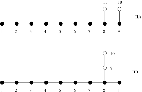
Figure 2: The Dynkin diagram of $E_{8}^{+++}$ drawn with an $A_{9}$ subalgebra (solid nodes) to yield a ten-dimensional theory.

IIA: First, consider the case where the gravity line is chosen as depicted in the top half of the figure. We will label the decomposition by a pair of non-negative integers $(l_{1},l_{2})$ where $l_{1}$ corresponds to the entry on the node denoted $11$ in the diagram and $l_{2}$ to the node denoted $10$. Doing the decomposition gives the $\mathfrak{sl}(10)$ content of table 2 on the first few levels.

$(l_{1},l_{2})$	$A_{9}$ weight	$E_{8}^{+++}$ element $\alpha$	$\alpha^{2}$	$ht(\alpha)$	$\mu$	Interpretation
(0,0)	[1,0,0,0,0,0,0,0,1]	(1,1,1,1,1,1,1,1,1,0,0)	2	9	1	$h_{a}{}^{b}$
(0,0)	[0,0,0,0,0,0,0,0,0]	(0,0,0,0,0,0,0,0,0,0,0)	0	0	1	$\phi$
(1,0)	[0,0,0,0,0,0,0,1,0]	(0,0,0,0,0,0,0,0,0,0,1)	2	1	1	$B_{(2)}$
(0,1)	[0,0,0,0,0,0,0,0,1]	(0,0,0,0,0,0,0,0,0,1,0)	2	1	1	$A_{(1)}$
(1,1)	[0,0,0,0,0,0,1,0,0]	(0,0,0,0,0,0,0,1,1,1,1)	2	4	1	$A_{(3)}$
(2,1)	[0,0,0,0,1,0,0,0,0]	(0,0,0,0,0,1,2,3,2,1,2)	2	11	1	$\tilde{A}_{(5)}$
(2,2)	[0,0,0,1,0,0,0,0,0]	(0,0,0,0,1,2,3,4,3,2,2)	2	17	1	$\tilde{B}_{(6)}$
(3,1)	[0,0,1,0,0,0,0,0,0]	(0,0,0,1,2,3,4,5,3,1,3)	2	22	1	$\tilde{A}_{(7)}$
(3,2)	[0,0,1,0,0,0,0,0,1]	(0,0,0,1,2,3,4,5,3,2,3)	2	23	1	$\tilde{A}_{(7,1)}$
(3,2)	[0,1,0,0,0,0,0,0,0]	(0,0,1,2,3,4,5,6,4,2,3)	0	30	1	$\tilde{A}^{\phi}_{(8)}$

Table 2: The first few levels of $E_{8}^{+++}$ decomposed with respect to its regular $A_{9}$ subalgebra obtained by deleting nodes $11$ and $10$ corresponding to a grading by $l_{1}$ and $l_{2}$ respectively. The representation content is related to type IIA supergravity in the text.

Looking at the fields, we find precisely the generators corresponding to the bosonic part of IIA supergravity, namely the NS-NS two-form, the RR one- and three-forms along with their duals. At level $(0,0)$ the generators of $\mathfrak{sl}(10)$ and two additional fields are found. As usual, they contain the gravitational degrees of freedom as $\mathfrak{gl}(10)$ and the additional scalar $\phi$ which can be interpreted as the dilaton field. Its dual occurs together with the dual gravity field at level $(3,2)$. The precise relation between the field generators in a non-linear realisation of eleven-dimensional supergravity and ten-dimensional IIA supergravity was already given in [6] and can be understood as follows: the positive root component of the $K^{a}{}_{11}$ generator that stretches in the eleventh dimension is interpreted as the Kaluza-Klein vector generator of the dimensionally reduced theory $K^{a}{}_{11}\sim R^{10}$. Similarly, the additional Cartan subalgebra scalar generator $\phi$ is proportional to the $K^{11}{}_{11}$ part. For the gauge field generators one finds canonically $R^{ab\,11}\sim R^{ab}$, where the former is the three-form of eleven-dimensional supergravity, while the latter is the 2-form generator in ten-dimensional IIA supergravity.

IIB: There is another possible regular $A_{9}$ subalgebra as shown in part (b) of figure 2, and its $\mathfrak{sl}(10)$ representation content is given in table 3 up to the level of the affine root.

$(l_{1},l_{2})$	$A_{9}$ weight	$E_{8}^{+++}$ element $\alpha$	$\alpha^{2}$	$ht(\alpha)$	$\mu$	Interpretation
(0,0)	[1,0,0,0,0,0,0,0,1]	(1,1,1,1,1,1,1,1,0,0,1)	2	9	1	$h_{a}{}^{b}$
(0,0)	[0,0,0,0,0,0,0,0,0]	(0,0,0,0,0,0,0,0,0,0,0)	0	0	1	$\phi$
(1,0)	[0,0,0,0,0,0,0,0,0]	(0,0,0,0,0,0,0,0,0,1,0)	2	1	1	$\chi$
(0,1)	[0,0,0,0,0,0,0,1,0]	(0,0,0,0,0,0,0,0,1,0,0)	2	1	1	$B_{(2)}$
(1,1)	[0,0,0,0,0,0,0,1,0]	(0,0,0,0,0,0,0,0,1,1,0)	2	2	1	$A_{(2)}$
(1,2)	[0,0,0,0,0,1,0,0,0]	(0,0,0,0,0,0,1,2,2,1,1)	2	7	1	$A_{(4)}$
(1,3)	[0,0,0,1,0,0,0,0,0]	(0,0,0,0,1,2,3,4,3,2,2)	2	16	1	$\tilde{B}_{(6)}$
(2,3)	[0,0,0,1,0,0,0,0,0]	(0,0,0,0,2,2,3,4,3,2,2)	2	17	1	$\tilde{A}_{(6)}$
(2,4)	[0,0,1,0,0,0,0,0,1]	(0,0,0,1,2,3,4,5,4,2,2)	2	23	1	$\tilde{A}_{(7,1)}$
(1,4)	[0,1,0,0,0,0,0,0,0]	(0,0,1,2,3,4,5,6,4,1,3)	2	29	1	$\tilde{A}^{\chi}_{(8)}$
(2,4)	[0,1,0,0,0,0,0,0,0]	(0,0,1,2,3,4,5,6,4,2,3)	0	30	1	$\tilde{A}^{\phi}_{(8)}$

Table 3: The first few levels of $E_{8}^{+++}$ decomposed with respect to its regular $A_{9}$ subalgebra obtained by deleting nodes $10$ and $9$ corresponding to a grading by $l_{1}$ and $l_{2}$ respectively. The representation content is related to type IIB supergravity in the text.

The last column gives the interpretation in terms of fields of IIB supergravity in ten dimensions. There is again a one-to-one correspondence if we accept that gauge fields and gravity have to be treated on an equal footing by introducing duals to either. Indeed, there is a non-linear realisation of IIB supergravity which employs all those fields [7]. The occurrence of only one four-form potential implies that its field strength will have to be self-dual.

More details on the higher levels for the IIA and IIB decompositions can be found in appendix A.1.

3.1.2 $E_{7}^{+++}$

The Dynkin diagram of very-extended $E_{7}$ is given in figure 3. Again, there are two alternative choices for the gravity subalgebra as the diagram has a bifurcation. As depicted in figure 3 we can choose either an $A_{9}$ or an $A_{7}$ subalgebra corresponding to theories in $8$ or $10$ dimensions respectively.

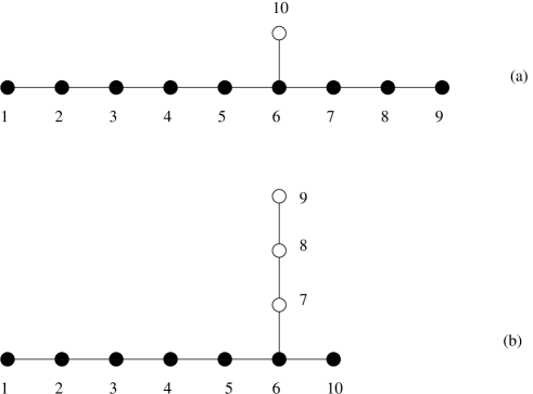
Figure 3: The Dynkin diagram of $E_{7}^{+++}$ drawn with an $A_{9}$ subalgebra to yield a ten-dimensional theory (a) or with an $A_{7}$ subalgebra to obtain an eight-dimensional theory (b).

(a) Decomposition into representations of $A_{9}$: A similar analysis to above gives the representation content with respect to $\mathfrak{sl}(10)$ presented in table 4 where we label the component on the node $10$ by $l$.

$l$	$A_{9}$ weight	$E_{7}^{+++}$ element $\alpha$	$\alpha^{2}$	$ht(\alpha)$	$\mu$	interpretation
0	[1,0,0,0,0,0,0,0,1]	(1,1,1,1,1,1,1,1,1,0)	2	9	1	$h_{a}{}^{b}$
1	[0,0,0,0,0,1,0,0,0]	(0,0,0,0,0,0,0,0,0,1)	2	1	1	$A_{(4)}$
2	[0,0,1,0,0,0,0,0,1]	(0,0,0,1,2,3,2,1,0,2)	2	11	1	$A_{(7,1)}$
2	[0,1,0,0,0,0,0,0,0]	(0,0,1,2,3,4,3,2,1,2)	0	18	0	$A_{(8)}^{\phi}$

Table 4: The first three levels of $E_{7}^{+++}$ decomposed with respect to its regular $A_{9}$ subalgebra.

All other representations lie above the level where the first affine root appears. We find a four-form ($l=1$) and the dual gravity generator ($l=2$) apart from the adjoint gravity generator at level $l=0$. This theory is a consistent non-supersymmetric truncation of IIB supergravity as can be easily found out by truncating the algebra called $g_{IIB}$ in [7]. We note that this theory is listed as the potential oxidation endpoint for the $E_{7}$ coset in [27]. We also note that a potential dual scalar (dual dilaton) has outer multiplicity zero ($\mu=0$) and is thus absent (and so is the dilaton itself). This is analogous to the eleven-dimensional case of $E_{8}^{+++}$.

The truncation of IIB to the content at hand can be understood purely algebraically by embedding $E_{7}^{+++}$ in $E_{8}^{+++}$. We choose as simple roots for the $E_{7}^{+++}$ subalgebra the gravity line and the element $\alpha_{7}+2\alpha_{8}+2\alpha_{9}+\alpha_{10}+\alpha_{11}$ of $E_{8}^{+++}$. From this embedding we see that the elements of $E_{8}^{+++}$ which also give rise to $E_{7}^{+++}$ generators must obey $2l_{1}=l_{2}$ in the type IIB table 3. The fields satisfying this constraint are the vielbein $h_{a}{}^{b}$, the Cartan subalgebra scalar $\phi$, a four-form potential $A_{(4)}$, the dual graviton $K^{a_{1}\ldots a_{7},b}$ and the field $A_{(8)}^{\phi}$ dual $\phi$. As the Cartan subalgebra of $E_{7}^{+++}$ has one dimension less than that of $E_{8}^{+++}$ it is clear that $\phi$ is absent in the $E_{7}^{+++}$ analysis and it is consistent that so is the dual field $A_{(8)}^{\phi}$. We also find that a reduction from IIA or eleven-dimensional supergravity is not immediately possible because of the different $A_{9}$ subalgebra.

(b) Decomposition into representations of $A_{7}$:

We can also consider embedding an $A_{7}$ subalgebra as indicated in part (b) of figure 3 where we expect to find an eight-dimensional theory. From the embedding $E_{7}^{+++}\subset E_{8}^{+++}$ we expect this to be a truncation of maximal $8d$ supergravity, not necessarily supersymmetric. We list all representations occurring up to the level of the affine $E_{7}^{+}$ root in table 5.

$(l_{1},l_{2},l_{3})$	$A_{7}$ weight	$E_{7}^{+++}$ element $\alpha$	$\alpha^{2}$	$ht(\alpha)$	$\mu$	interpretation
(0,0,0)	[1,0,0,0,0,0,1]	(1,1,1,1,1,1,0,0,0,1)	2	7	1	$h_{a}{}^{b}$
(0,0,0)	[0,0,0,0,0,0,0]	(0,0,0,0,0,0,0,0,0,0)	0	0	2	$\phi$
(1,0,0)	[0,0,0,0,0,0,0]	(0,0,0,0,0,0,0,0,1,0)	2	1	1	$\chi$
(0,1,0)	[0,0,0,0,0,0,0]	(0,0,0,0,0,0,0,1,0,0)	2	1	1	$\chi$
(0,0,1)	[0,0,0,0,0,1,0]	(0,0,0,0,0,0,1,0,0,0)	2	1	1	$A_{(2)}$
(1,1,0)	[0,0,0,0,0,0,0]	(0,0,0,0,0,0,0,1,1,0)	2	2	1	$\chi$
(0,1,1)	[0,0,0,0,0,1,0]	(0,0,0,0,0,0,1,1,0,0)	2	2	1	$A_{(2)}$
(1,1,1)	[0,0,0,0,0,1,0]	(0,0,0,0,0,0,1,1,1,0)	2	3	1	$A_{(2)}$
(0,1,2)	[0,0,0,1,0,0,0]	(0,0,0,0,1,2,2,1,0,1)	2	7	1	$\tilde{A}_{(4)}$
(1,1,2)	[0,0,0,1,0,0,0]	(0,0,0,0,1,2,2,1,1,1)	2	8	1	$\tilde{A}_{(4)}$
(1,2,2)	[0,0,0,1,0,0,0]	(0,0,0,0,1,2,2,2,1,1)	2	9	1	$\tilde{A}_{(4)}$
(1,2,3)	[0,0,1,0,0,0,1]	(0,0,0,1,2,3,3,2,1,1)	2	13	1	$\tilde{A}_{(5,1)}$
(0,1,3)	[0,1,0,0,0,0,0]	(0,0,1,2,3,4,3,1,0,2)	2	16	1	$\tilde{A}_{(6)}^{\chi}$
(1,1,3)	[0,1,0,0,0,0,0]	(0,0,1,2,3,4,3,1,1,2)	2	17	1	$\tilde{A}_{(6)}^{\chi}$
(0,2,3)	[0,1,0,0,0,0,0]	(0,0,1,2,3,4,3,2,0,2)	2	17	1	$\tilde{A}_{(6)}^{\chi}$
(1,2,3)	[0,1,0,0,0,0,0]	(0,0,1,2,3,4,3,2,1,2)	0	18	2	$\tilde{A}_{(6)}^{\phi}$

Table 5: The first three levels of $E_{7}^{+++}$ decomposed with respect to its regular $A_{7}$ subalgebra of figure 3. $l_{1},l_{2}$ and $l_{3}$ correspond to nodes 9, 8 and 7 respectively.

We find a triplet of positive root scalars and two Cartan subalgebra scalars, the vielbein, and the duals of all these fields (note outer multiplicity 2 for the dual dilaton). There are also three two-forms with their dual four-forms. This is the field content of a non-supersymmetric truncation of maximal ${\cal N}=2$ eight-dimensional supergravity whose bosonic field content comprises a vielbein, a triplet of two-forms, a triplet of one-forms, one three-form potential and an additional (axion) scalar. These fields arise from reduction of the maximal eleven-dimensional theory and so transform under a global $SL(3)$. Furthermore the supergravity theory has scalars in the coset $SL(3)/SO(3)$.

The rôle of the global $SL(3)$ can also be seen already in the Dynkin diagram of $E_{7}^{+++}$ where we have an $A_{2}$ which is not attached to the gravity line, consisting of the nodes labelled $8$ and $9$ in diagram 3.1.2, part (b). In the non-linear realisation, the fields are controlled by the coset of $E_{7}^{+++}$ by its Chevalley invariant subalgebra and the coset contains a part belonging to this $A_{2}$ which is just $SL(3)/SO(3)$ after exponentiation of the real algebras and acts on the scalars arising from this part of the algebra in the decomposition. The coset is parametrised by five elements and three are associated with positve roots of $E_{7}^{+++}$ and two with the Cartan subalgebra as is also apparent in the table. The positive roots of the $A_{2}$ subalgebra also act on the generators forming the two-form representation on level $(0,0,1)$ in the table and so generate another two two-forms, all of which transform under the $\mathfrak{sl}(3)$. These fields together with the vielbein are retained in the non-supersymmetric truncation of maximal ${\cal N}=2$ eight-dimensional supergravity. Again the Kac-Moody algebra also contains duals of all the fields precisely up to the level of the first affine root.

In appendix A.2 we list details for the higher levels of a decomposition of $E_{7}^{+++}$ with respect to its regular $A_{8}$ gravity subalgebra, corresponding to a nine-dimensional theory.

3.1.3 $E_{6}^{+++}$

This section deals with very-extended $E_{6}$ which is denoted by $E_{6}^{+++}$. The Dynkin diagram is given in figure 4. Here there is only one canonical maximal choice of a gravity subalgebra $A_{7}$ because the possibilities are exchanged by a diagram automorphism. The list of resulting representations of $\mathfrak{sl}(8)$ up to level $(1,2)$ (first affine root) is provided in table 6. The level $(l_{1},l_{2})$ corresponds to the components of a positive root on the nodes $9$ and $8$ respectively.

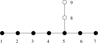
Figure 4: The Dynkin diagram of $E_{6}^{+++}$ drawn with its $A_{7}$ subalgebra.

$(l_{1},l_{2})$	$A_{7}$ weight	$E_{6}^{+++}$ element $\alpha$	$\alpha^{2}$	$ht(\alpha)$	$\mu$	Interpretation
(0,0)	[1,0,0,0,0,0,1]	(1,1,1,1,1,1,1,0,0)	2	7	1	$h_{a}{}^{b}$
(0,0)	[0,0,0,0,0,0,0]	(0,0,0,0,0,0,0,0,0)	0	0	1	$\phi$
(1,0)	[0,0,0,0,0,0,0]	(0,0,0,0,0,0,0,0,1)	2	1	1	$\chi$
(0,1)	[0,0,0,0,1,0,0]	(0,0,0,0,0,0,0,1,0)	2	1	1	$A_{(3)}$
(1,1)	[0,0,0,0,1,0,0]	(0,0,0,0,0,0,0,1,1)	2	2	1	$\tilde{A}_{(3)}$
(1,2)	[0,0,1,0,0,0,1]	(0,0,0,1,2,1,0,2,1)	2	7	1	$\tilde{A}_{(5,1)}$
(0,2)	[0,1,0,0,0,0,0]	(0,0,1,2,3,2,1,2,0)	2	11	1	$\tilde{A}^{\chi}_{(6)}$
(1,2)	[0,1,0,0,0,0,0]	(0,0,1,2,3,2,1,2,1)	0	12	1	$\tilde{A}^{\phi}_{(6)}$

Table 6: The first few levels of $E_{6}^{+++}$ decomposed with respect to its regular $A_{7}$ subalgebra obtained by deleting nodes $9$ and $8$ corresponding to a grading by $l_{1}$ and $l_{2}$ respectively.

We find a positive root scalar (axion) and its dual, but also the vielbein and a Cartan subalgebra scalar (dilaton) on level $(0,0)$ and their duals. There also are two three-forms generated by positive roots. The dual graviton and dual dilaton occur on the same level. This is precisely the field content of the oxidation endpoint of the supersymmetric $E_{6}$ coset theory described in [27] where the four-form field strength and its dual form a doublet under a global $SL(2,\mathbf{R})$. Details on the higher levels can be found in appendix A.3.

3.2 $D$ series

The Dynkin diagram of the very-extended $D$ algebras is given in figure 5 and the gravity line is indicated as usual by the solid nodes. Different from the cases considered so far, there are actually two nodes in the gravity subalgebra where other subalgebras couple to it. The gravity line is an $A_{n-2}$ algebra, and we expand around the nodes marked as $n$ and $n-1$. Expanding the node $n$ leaves a $D_{n-1}$ subalgebra, further expansion around $n-1$ yields $A_{n-2}$. If the expansion nodes are exchanged then we get a $E_{7}^{+(n-8)}$ by which we mean an $E_{7}$ algebra extended $n-8$ times. This is an indefinite Kac-Moody algebra, and belongs to the class of algebras considered in [13] but is in general not very-extended.

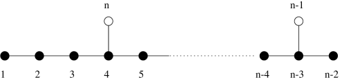
Figure 5: The Dynkin diagram of $D_{n-3}^{+++}$ drawn with its $A_{n-2}$ subalgebra as gravity given by the solid nodes.

According to the level criterion for the physical spectrum of ${\cal O}_{\mathfrak{g}}$, we are interested in finding all representations on levels less than $(1,1)$ which is the level of the affine root coming from the affine $D_{n-3}$ subalgebra. It is possible to apply a mild generalisation of the Feingold-Frenkel method to find the decomposition up to this level and the result is presented in table 7. This list is complete since the tensor product of the representations at levels $(0,1)$ and $(1,0)$ has three summands, one of which lies in the ideal described in section 2.2 and thus has to be removed. The other two are the listed ones. The outer multiplicity of the first one is fixed by it being generated by the lowest element on that level and being a real root. The outer multiplicity of the affine $D$ root can be computed by noting that its multiplicity in the algebra is $n-3$ and its multiplicity as a weight in the other representation on that level is $n-4$.

$(l_{1},l_{2})$	$A_{n-2}$ weight	$D_{n-3}^{+++}$ element $\alpha$	$\alpha^{2}$	$ht(\alpha)$	$\mu$
(0,0)	[1,0,0,0,0,…,0,0,1]	(1,1,1,1,…,1,1,0,0)	2	$n-2$	1	$h_{a}{}^{b}$
(0,0)	[0,0,0,0,0,…,0,0,0]	(0,0,0,0,…,0,0,0,0)	0	0	1	$\phi$
(0,1)	[0,0,0,0,0,…,0,1,0]	(0,0,0,0,…,0,0,1,0)	2	1	1	$A_{(2)}$
(1,0)	[0,0,0,1,0,…,0,0,0]	(0,0,0,0,…,0,0,0,1)	2	1	1	$\tilde{A}_{(n-5)}$
(1,1)	[0,0,1,0,0,…,0,0,1]	(0,0,0,1,…,1,0,1,1)	2	$n-4$	1	$\tilde{A}_{(n-4,1)}$
(1,1)	[0,1,0,0,0,…,0,0,0]	(0,0,1,2,…,2,1,1,1)	0	$2n-8$	1	$\tilde{A}_{(n-3)}^{\phi}$

Table 7: The first levels of $D_{n-3}^{+++}$ decomposed with respect to its regular $A_{n-2}$ subalgebra obtained by deleting nodes $n$ and $n-1$ giving a grading by $l_{1}$ and $l_{2}$ respectively.

The field content on these levels is thus a vielbein in $n-1$ dimensions, a scalar coming from the Cartan subalgebra which we interpret as dilaton and an antisymmetric two-form. Furthermore we find the duals to all these fields. This is just the set of massless states of closed bosonic string theory in $n-1$ dimensions, in agreement with the conjecture in [6] and also in agreement with the content of the oxidised theory [27]. We also note that the Dynkin diagram has a bifurcation at node $4$ and the other choice of gravity $A_{5}$ subalgebra would lead to a theory in six dimensions. The field content up to the level of the affine root of that theory exists of $(n-6)(n-7)$ positive root scalars and their duals, $2(n-6)$ 2-forms, $n-6$ Cartan subalgebra scalars and their duals, along with a dual graviton.

In appendix A.4 we list the higher levels for the particular case of $D_{8}^{+++}$.

3.3 $A$ series

In this section we analyse the very-extended algebras of the $A$ series on level one which is the relevant bound for the spectrum as the first affine root occurs at this level. The Dynkin diagram of $A_{n-3}^{+++}$ is given in figure 6.

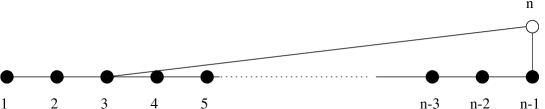
Figure 6: The Dynkin diagram of $A_{n-3}^{+++}$ drawn with its $A_{n-1}$ subalgebra as gravity.

The representation content with respect to the indicated $A_{n-1}$ subalgebra was presented in [18] based on an analysis of the possible weights and the Serre relations. Here we deduce the same results using the Feingold-Frenkel mechanism (see section 2). Table 8 contains the results and all other representations occur at higher level.

$l$	$A_{n-1}$ weight	$A_{n-3}^{+++}$ element $\alpha$	$\alpha^{2}$	$ht(\alpha)$	$\mu$	Interpretation
0	[1,0,0,0,…,0,1]	(1,1,1,…,1,0)	2	$n-1$	1	$h_{a}{}^{b}$
1	[0,0,1,0,…,0,1]	(0,0,0,…,0,1)	2	1	1	$\tilde{A}_{(n-3,1)}$
1	[0,1,0,0,…,0,0]	(0,0,1,…,1,1)	0	$n-2$	0	$\tilde{A}_{(n-2)}$

Table 8: The first level of $A_{n-3}^{+++}$ decomposed with respect to its regular $A_{n-1}$ subalgebra obtained by deleting node $n$ which gives rise to a grading by $l$.

We have included the dual of a (Cartan subalgebra) scalar which is an allowed representation but with vanishing outer multiplicity as we know from section 2. Hence, very-extended $A^{+++}_{n-3}$ only contains the graviton field and its dual. This supports the claim of [18] that this algebra lies behind a non-linear realisation of pure gravity in $n$ dimensions. The content is in agreement with the oxidised theory which is pure Einstein-Hilbert theory [27]. We propose a general result for level $2$ in the appendix A.5 which is also a non-trivial result about the general structure of this family of very-extended Kac-Moody algebras.

4 Non simply-laced cases

We next turn to the study of very-extended algebras that derive from classical algebras which are not simply-laced, starting with the exceptional cases. Afterwards, the families of very-extended algebras belonging to the $B$ and the $C$ series will be considered.

4.1 $F_{4}^{+++}$

The Dynkin diagram of $F_{4}^{+++}$ is depicted in figure 7. The maximal gravity subalgebra is five-dimensional and so the fields will be representations of $\mathfrak{sl}(6)$. The list of representations occuring up to level $(2,4)$ (which is the level of the affine root in affinised $F_{4}$) is in table 9. The lengths of the roots are normalised such that long roots have norm square 2.

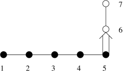
Figure 7: The Dynkin diagram of $F_{4}^{+++}$ drawn with its $A_{5}$ subalgebra as gravity given by the solid nodes.

$(l_{1},l_{2})$	$A_{5}$ weight	$F_{4}^{+++}$ element $\alpha$	$\alpha^{2}$	$ht(\alpha)$	$\mu$	Interpretation
(0,0)	[1,0,0,0,1]	(1,1,1,1,1,0,0)	2	5	1	$h_{a}{}^{b}$
(0,0)	[0,0,0,0,0]	(0,0,0,0,0,0,0)	0	0	1	$\phi$
(1,0)	[0,0,0,0,0]	(0,0,0,0,0,0,1)	1	1	1	$\chi$
(0,1)	[0,0,0,0,1]	(0,0,0,0,0,1,0)	1	1	1	$A_{(1)}$
(1,1)	[0,0,0,0,1]	(0,0,0,0,0,1,1)	1	2	1	$A_{(1)}$
(0,2)	[0,0,0,1,0]	(0,0,0,0,1,2,0)	2	3	1	$A_{(2)}$
(1,2)	[0,0,0,1,0]	(0,0,0,0,1,2,1)	1	4	1	$A_{(2)}$
(2,2)	[0,0,0,1,0]	(0,0,0,0,1,2,2)	2	5	1	$A_{(2)}$
(1,3)	[0,0,1,0,0]	(0,0,0,1,2,3,1)	1	7	1	$\tilde{A}_{(3)}$
(2,3)	[0,0,1,0,0]	(0,0,0,1,2,3,2)	1	8	1	$\tilde{A}_{(3)}$
(2,4)	[0,0,1,0,1]	(0,0,0,1,2,4,2)	2	9	1	$\tilde{A}_{(3,1)}$
(1,4)	[0,1,0,0,0]	(0,0,1,2,3,4,1)	1	11	1	$\tilde{A}_{(4)}^{\chi}$
(2,4)	[0,1,0,0,0]	(0,0,1,2,3,4,2)	0	12	1	$\tilde{A}_{(4)}^{\phi}$

Table 9: The first levels of $F_{4}^{+++}$ decomposed with respect to its regular $A_{5}$ subalgebra obtained by deleting nodes $7$ and $6$ giving a grading by $l_{1}$ and $l_{2}$ respectively.

Examining the table we find that the fields up to and including the level of the affine root consist of gravity $h_{a}{}^{b}$ and a scalar $\phi$ on level $(0,0)$, where $\phi$ lives in the Cartan subalgebra. On the positive levels we find two one-form fields, and one two-form field all together with their duals as well as one further two-form whose field strength is self-dual. This self-duality follows from the listed fields as we have three two-form fields of which at most two may be paired together to form a gauge field whose field strength has no self-duality condition. This content is the field content of the $F_{4}^{+++}$ oxidised theory listed in [27].

It is useful to precisely identify this theory. The bosonic content of the (1,0) supersymmetry multiplets in six dimensions are as follows; the supergravity mulitplet which has a graviton and second rank tensor gauge field, the vector multiplet which has just a vector gauge field and finally the tensor multiplet which has a scalar and a second rank tensor gauge field. Both of the second rank tensor gauge fields have field strengths that are self-dual with the one in the gravity multiplet being of opposite self-duality to that in the tensor multiplet. As such, it is clear that the $F_{4}^{+++}$ theory consist of supergravity coupled to two vector multiplets and two tensor multiplets. The coupling of these multiplets is given in [28].

4.2 $G_{2}^{+++}$

The Dynkin diagram of very extended $G_{2}$ is shown in figure 8 and we list the representations in table 10 up to height $6$.

Figure 8: The Dynkin diagram of $G_{2}^{+++}$ drawn with its $A_{4}$ subalgebra as gravity given by the solid nodes.

$l$	$A_{4}$ weight	$G_{2}^{+++}$ element $\alpha$	$\alpha^{2}$	$ht(\alpha)$	$\mu$	Interpretation
0	[1,0,0,1]	(1,1,1,1,0)	2	4	1	$h_{a}{}^{b}$
1	[0,0,0,1]	(0,0,0,0,1)	2	1	1	$A_{(1)}$
2	[0,0,1,0]	(0,0,0,1,2)	2	3	1	$\tilde{A}_{(2)}$
3	[0,0,1,1]	(0,0,0,1,3)	6	4	1	$\tilde{A}_{(2,1)}$
3	[0,1,0,0]	(0,0,1,2,3)	0	6	0	$\tilde{A}_{(3)}^{\phi}$

Table 10: The first levels of $G_{2}^{+++}$ decomposed with respect to its regular $A_{4}$ subalgebra obtained by deleting nodes $5$ corresponding to a grading by $l$.

All other representations occur at higher level. We see that we have a five-dimensional theory with a gravitational field and its dual and also a 1-form and its dual. This is the right bosonic field content for Einstein-Maxwell theory or $N=2$ supergravity in five dimensions [27]. We list higher levels in appendix A.7.

4.3 $B$ series

The Dynkin diagram of $B_{n-3}^{+++}$ is depicted in figure 9. Similar to the $D$ series we face the problem of expanding about two nodes but we can again apply our low-level techniques to get the representations up to the level of the affine root of the $B$ series. We denote the level as indicated in the Dynkin diagram by $(l_{1},l_{2})$ corresponding to the entries on the nodes $n$ and $n-1$ respectively. The affine root is the element $(0,0,1,2,2,\dots,2,1)$ in $B_{n-3}^{+++}$ which is at level $(1,2)$ and so we have to construct the representations up to this level. By similar arguments to section 3.2 and taking antisymmetry into account we find table 11.

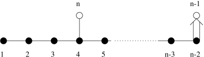
Figure 9: The Dynkin diagram of $B_{n-3}^{+++}$ drawn with its $A_{n-2}$ subalgebra as gravity given by the solid nodes.

$(l_{1},l_{2})$	$A_{n-2}$ weight	$B_{n-3}^{+++}$ element $\alpha$	$\alpha^{2}$	$ht(\alpha)$	$\mu$
(0,0)	[1,0,0,0,0,…,0,0,1]	(1,1,1,1,…,1,0,0)	2	$n-2$	1	$h_{a}{}^{b}$
(0,0)	[0,0,0,0,0,…,0,0,0]	(0,0,0,0,…,0,0,0)	0	0	1	$\phi$
(0,1)	[0,0,0,0,0,…,0,0,1]	(0,0,0,0,…,0,1,0)	1	1	1	$A_{(1)}$
(0,2)	[0,0,0,0,0,…,0,1,0]	(0,0,0,0,…,1,2,0)	2	3	1	$A_{(2)}$
(1,0)	[0,0,0,1,0,…,0,0,0]	(0,0,0,0,…,0,0,1)	2	1	1	$\tilde{A}_{(n-5)}$
(1,1)	[0,0,1,0,0,…,0,0,0]	(0,0,0,1,…,1,1,1)	1	$n-3$	1	$\tilde{A}_{(n-4)}$
(1,2)	[0,0,1,0,0,…,0,0,1]	(0,0,0,1,…,1,2,1)	2	$n-2$	1	$\tilde{A}_{(n-4,1)}$
(1,2)	[0,1,0,0,0,…,0,0,0]	(0,0,1,2,…,2,2,1)	0	$2n-6$	1	$\tilde{A}_{(n-3)}^{\phi}$

Table 11: The first levels of $B_{n-3}^{+++}$ decomposed with respect to its regular $A_{n-2}$ subalgebra obtained by deleting nodes $n$ and $n-1$ giving a grading by $l_{1}$ and $l_{2}$ respectively.

The field content up to the relevant level is thus a 1-form, a 2-form, the metric and a dilaton and their duals, forming part of an $(n-1)$-dimensional theory. This field content agrees with the oxidised theory considered in [27]. In ten dimensions it is just the bosonic field content of $N=1$ supergravity plus one abelian vector multiplet. The non-linear realisation has been studied in [29]. Again, there should be a different theory from the bifurcation in the Dynkin diagram. The case of $B_{3}^{+++}$ proves to be interesting and is analysed at higher levels in appendix A.8.

4.4 $C$ series

The prescription for finding the field content of a tentative physical theory applied to $C_{n-3}^{+++}$ tells us that we should start by considering its $A_{3}$ subalgebra as indicated in figure 10.

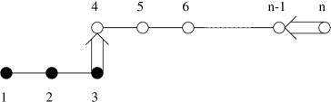
Figure 10: The Dynkin diagram of $C_{n-3}^{+++}$ drawn with its $A_{3}$ subalgebra as gravity given by the solid nodes.

We see that there is a $C_{n-3}$ subalgebra coupled via (the affine) node $3$ to this $A_{3}$ and so from the structure of $C_{n-3}$ this tells us that there will be $(n-4)^{2}$ scalar fields and their duals two-forms and $2n-8$ one-forms. We also find the metric and $n-4$ dilatons and their dual fields up to the level of the affine $C$ root. This agrees with the results in [27]. We do not list higher levels for any $C$ series case because of lack of space and the large number of fields already at low levels.

5 Discussion

5.1 The $A_{d-3}^{+++}$ subalgebras

The theories ${\cal V}_{\mathfrak{g}}$ based on the very-extended Kac-Moody algebras ${\mathfrak{g}}^{+++}$ all contain a gravitational sector. It has been conjectured that pure gravity in $d$-dimensional space-time can be extended such that it is a non-linear realisation based on $A_{d-3}^{+++}$ i.e ${\cal V}_{A_{d-3}}$. To be consistent we would therefore have to find that $A_{d-3}^{+++}$ is contained in ${\mathfrak{g}}^{+++}$ for the appropriate $d$. This is known to be true for $E_{8}^{+++}$ [18], but we now show it is true in all cases. This can be understood by recalling Dynkin’s construction of all regular semi-simple subalgebras of ${\mathfrak{g}}$. We begin considering the Dynkin diagram of the non-twisted affine ${\mathfrak{g}}^{+}$ and deleting nodes from it [30]. If we want to consider ${\cal V}_{\mathfrak{g}}$ as a $d$-dimensional theory then we can find an $A_{d-1}$ regular subalgebra in ${\mathfrak{g}}^{+++}$ which starts at the very-extended node. By removing the over- and the very-extended node we obtain a $A_{d-3}$ subalgebra of ${\mathfrak{g}}^{+++}$. This is actually a subalgebra of ${\mathfrak{g}}^{+}$ whose Dynkin diagram is a subdiagram of the non-twisted affine one and due to Dynkin’s construction it is thus a subalgebra of ${\mathfrak{g}}$. Now we just have to very-extend both ${\mathfrak{g}}$ and this $A_{d-3}$ to find that there exists $A_{d-3}^{+++}\subset{\mathfrak{g}}^{+++}$. Explicitly, we take as the simple root extending $A_{d-1}$ to $A_{d-3}^{+++}$ the element generating the dual graviton. It is encouraging that the non-linear realisation of ${\cal V}_{\mathfrak{g}}$ contains the expected ${\cal V}_{A_{d-3}}$.

We also note that table 8 tells us that if there are Cartan subalgebra scalars $\phi$, their duals $A_{(d-2)}^{\phi}$ will come in at the same level as the dual graviton. This has been observed in the case by case analysis too.

5.2 T-duality and bifurcations

In this section we propose a connection between the bifurcations (or T-junctions) of the Dynkin diagram and a generalisation of T-duality transformations in the theory of gravity and matter associated with it. Suppose we are given a certain very-extended algebra ${\mathfrak{g}}^{+++}$ with a choice of gravity subalgebra $A_{d-1}$. Then Kaluza-Klein reductions can be realised by shortening the gravity subalgebra by a node from the far end because this corresponds to decomposing tensors of $\mathfrak{gl}(d)$ into tensors of $\mathfrak{gl}(d-1)$. For example, this is how the content of the IIA decomposition of $E_{8}^{+++}$ can be obtained from the $11d$ decomposition of $E_{8}^{+++}$, cf. figures 1 and 2. If the Dynkin diagram of ${\mathfrak{g}}^{+++}$ contains a bifurcation and our gravity subalgebra, called $A_{d_{A}-1}$, stretches past it, it is possible to reduce the theory down to the point of the bifurcation. The spectrum obtained then will coincide with the spectrum of any other choice of gravity subalgebra $A_{d_{B}-1}$ stretching past the bifurcation, subsequently reduced to the bifurcation point.

For example, the $E_{8}^{+++}$ diagram has a bifurcation point and so we can take different embeddings of gravity subalgebras and the theories agree if reduced to nine dimensions. In particular, there are two choices of $A_{9}$ subalgebra stretching past the bifurcation point and the field contents of the different decompositions have been related to IIA and IIB supergravity in section 3.1.1. This agrees with the well-known feature of the two maximal ten-dimensional supergravity theories that they are related by a T-duality if each is compactified on a circle. In this case the bifurcation in the Dynkin diagrams gives rise to theories which are related by some generalised T-duality transforms if dimensionally reduced down to the bifurcation point. The proposal that $E_{8}^{+++}$ is a symmetry not only of $11d$ supergravity but also of M-theory and thus of its $10d$ superstring limit is consistent with this observation because it is well-known that T-duality lifts to string theory.

In a similar way we can look at the $E_{7}^{+++}$. The bifurcation point is the node labelled $6$ in figure 3 and so we expect two theories which agree when reduced to seven dimensions. One corresponds to the maximal ten-dimensional theory, called interpretation (a) in section 3.1.2 while the other is the eight-dimensional interpretation (b). Naturally, both reduced theories are contained in the decomposition of $E_{8}^{+++}$ into its $A_{6}$ subalgebra.

A similar proposal for generalising T-duality has been put forward in [31].

5.3 Concluding remarks

We have used the very-extended Kac-Moody algebras ${\mathfrak{g}}^{+++}$ to introduce a set of theories ${\cal V}_{\mathfrak{g}}$ which are just the non-linear realisation based on ${\mathfrak{g}}^{+++}$. We might expect that the theories ${\cal V}_{\mathfrak{g}}$ contain the oxidised theories ${\cal O}_{\mathfrak{g}}$ as subsectors since the latter by construction have a symmetry group ${\mathfrak{g}}$ in three dimensions. In this paper we have calculated the $A_{d-1}$ representations of ${\mathfrak{g}}^{+++}$ at low levels and so deduced the field content of ${\cal V}_{\mathfrak{g}}$. It was found that the fields of the theory ${\cal V}_{\mathfrak{g}}$ up to the level of the affine root contain the fields of ${\cal O}_{\mathfrak{g}}$ in the correct representation of $A_{d-1}$. This implies that the field content of the theories ${\cal O}_{\mathfrak{g}}$ can be read off from the Dynkin diagram, particularly simple at level $1$. We have also argued that the Dynkin diagram encodes information about generalised T-dualities.

While it is an important consistency check that the field contents match between ${\cal V}_{\mathfrak{g}}$ and ${\cal O}_{\mathfrak{g}}$ at low levels, it is an important task to further uncover the structure of the full ${\cal V}_{\mathfrak{g}}$ which includes finding the correct dynamical equations for the higher level fields, as listed in the appendices, which are expected to be largely governed by the structure of ${\mathfrak{g}}^{+++}$.

In this way of viewing things considered here, gravity can be embedded in a larger theory in a number of different ways, some of which involve no supersymmetry. For example, in any space-time dimension, $d$, gravity appears as part of the theories ${\cal V}_{A_{d-3}}$ and ${\cal V}_{D_{d-2}}$. At low energy, in the former theory one only has gravity, but in the latter one also has a dilaton and a second rank tensor gauge field and in both of these theories one might expect to see an infinite number of massive modes corresponding to the infinite number of generators in the Kac-Moody algebra. In certain other dimensions, for example, in ten and eleven dimensions one has further possiblilties such as the theories associated with ${\cal V}_{E_{8}}$.

It is instructive to realise that all the theories that have been thought to play a part in a unified theory of physics are included in this picture based on very-extended Kac-Moody algebras and it is natural to suppose that they are all part of some larger algebraic structure that may be a Borcherds algebra. This idea is consistent with the old suggestion [32, 33] that the closed bosonic string might contain the superstrings. An encouraging sign is that $D_{24}^{+++}$ contains $E_{8}^{+++}\times D_{16}$ if one includes the weight lattice of the former [34].

The suggestion given above fits naturally into the historical developments to find a unified theory. Although supergravity in the late 1970s and early 1980s was hoped to provide a unified theory of gravity and quantum theory it was realised in the mid 1980s that embedding these theories in, the previously discovered, superstrings was more likely to be successful. However, by the late 1990s it became clear that superstring theories themselves were but part of some bigger structure which was called M theory. From the perspective of the above suggestion, M theory is itself just one step on the way and that the very-extended algebras play an important rôle in fixing the structure of that theory, similar to supersymmetry. The final algebraic structure may include Borcherds’ Fake Monster algebra which is the vertex algebra on the unique even, self-dual Lorentzian lattice in $26$ dimensions [35]. Its Dynkin diagram contains an infinite number of nodes and it has been studied in the context of string scattering amplitudes in [36].

Finally we note that at present, the theories ${\cal V}_{\mathfrak{g}}$ have been introduced as non-linear realisations, very much along the same lines as elementary particles where modelled in the early days before this was understood as the breaking of a symmetry. It seems interesting to consider what the unbroken theory looks like for ${\cal V}_{\mathfrak{g}}$.

Acknowledgements
We are grateful for discussions with P. Goddard and M. R. Gaberdiel. AK would like to thank King’s College, London, for hospitality and the EPSRC and the Studienstiftung des deutschen Volkes for financial support. IS is grateful for the support by the Israel Academy of Science and Humanities - Centers of Excellence Program, and the German-Israel Bi-National Science Foundation. This research was supported in part by the PPARC grants PPA/G/O/2000/00451 and PPA/G/S4/1998/00613.

Appendix A Some results on higher levels

In the appendices we list results obtained on the field contents of the theories ${\cal V}_{\mathfrak{g}}$ if read in terms of the indicated $A$ subalgebras. Most of the results were obtained with the help of a computer and give a flavour of the structure of ${\mathfrak{g}}^{+++}$ at higher level. Lack of space prevents us from presenting more data.

A.1 IIA and IIB theories from $E_{8}^{+++}$

The higher levels of the decomposition of $E_{8}^{+++}$ with respect to its $A_{10}$ subalgebra are well-documented in the literature [19] to which we refer the reader. Here we give higher levels of the two decompositions into $A_{9}$ subalgebras discussed in the section 3.1.1.

IIA: This is the data obtained for the IIA case. All the listed levels are complete.

$(l_{1},l_{2})$	$A_{9}$ weight	$E_{8}^{+++}$ element $\alpha$	$\alpha^{2}$	$ht(\alpha)$	$\mu$
(1,0)	[0,0,0,0,0,0,0,1,0]	(0,0,0,0,0,0,0,0,0,0,1)	2	1	1
(0,1)	[0,0,0,0,0,0,0,0,1]	(0,0,0,0,0,0,0,0,0,1,0)	2	1	1
(1,1)	[0,0,0,0,0,0,1,0,0]	(0,0,0,0,0,0,0,1,1,1,1)	2	4	1
(2,1)	[0,0,0,0,1,0,0,0,0]	(0,0,0,0,0,1,2,3,2,1,2)	2	11	1
(3,1)	[0,0,1,0,0,0,0,0,0]	(0,0,0,1,2,3,4,5,3,1,3)	2	22	1
(4,1)	[1,0,0,0,0,0,0,0,0]	(0,1,2,3,4,5,6,7,4,1,4)	2	37	1
(2,2)	[0,0,0,1,0,0,0,0,0]	(0,0,0,0,1,2,3,4,3,2,2)	2	17	1
(3,2)	[0,0,1,0,0,0,0,0,1]	(0,0,0,1,2,3,4,5,3,2,3)	2	23	1
(3,2)	[0,1,0,0,0,0,0,0,0]	(0,0,1,2,3,4,5,6,4,2,3)	0	30	1
(4,2)	[0,1,0,0,0,0,0,1,0]	(0,0,1,2,3,4,5,6,4,2,4)	2	31	1
(4,2)	[1,0,0,0,0,0,0,0,1]	(0,1,2,3,4,5,6,7,4,2,4)	0	38	1
(4,2)	[0,0,0,0,0,0,0,0,0]	(1,2,3,4,5,6,7,8,5,2,4)	-2	47	2
(5,2)	[1,0,0,0,0,0,1,0,0]	(0,1,2,3,4,5,6,8,5,2,5)	2	41	1
(5,2)	[0,0,0,0,0,0,0,1,0]	(1,2,3,4,5,6,7,8,5,2,5)	0	48	1
(6,2)	[0,0,0,0,0,1,0,0,0]	(1,2,3,4,5,6,8,10,6,2,6)	2	53	1
(3,3)	[0,1,0,0,0,0,0,0,1]	(0,0,1,2,3,4,5,6,4,3,3)	2	31	1
(3,3)	[1,0,0,0,0,0,0,0,0]	(0,1,2,3,4,5,6,7,5,3,3)	0	39	0
(4,3)	[0,1,0,0,0,0,1,0,0]	(0,0,1,2,3,4,5,7,5,3,4)	2	34	1
(4,3)	[1,0,0,0,0,0,0,0,2]	(0,1,2,3,4,5,6,7,4,3,4)	2	39	1
(4,3)	[1,0,0,0,0,0,0,1,0]	(0,1,2,3,4,5,6,7,5,3,4)	0	40	1
(4,3)	[0,0,0,0,0,0,0,0,1]	(1,2,3,4,5,6,7,8,5,3,4)	-2	48	2
(5,3)	[0,1,0,0,1,0,0,0,0]	(0,0,1,2,3,5,7,9,6,3,5)	2	41	1
(5,3)	[1,0,0,0,0,0,1,0,1]	(0,1,2,3,4,5,6,8,5,3,5)	2	42	1
(5,3)	[1,0,0,0,0,1,0,0,0]	(0,1,2,3,4,5,7,9,6,3,5)	0	45	1
(5,3)	[0,0,0,0,0,0,0,1,1]	(1,2,3,4,5,6,7,8,5,3,5)	0	49	1
(5,3)	[0,0,0,0,0,0,1,0,0]	(1,2,3,4,5,6,7,9,6,3,5)	-2	51	3
(4,4)	[1,0,0,0,0,0,1,0,0]	(0,1,2,3,4,5,6,8,6,4,4)	2	43	1
(4,4)	[0,0,0,0,0,0,0,0,2]	(1,2,3,4,5,6,7,8,5,4,4)	2	49	1
(4,4)	[0,0,0,0,0,0,0,1,0]	(1,2,3,4,5,6,7,8,6,4,4)	0	50	0
(5,4)	[1,0,0,0,0,1,0,0,1]	(0,1,2,3,4,5,7,9,6,4,5)	2	46	1
(5,4)	[0,1,0,1,0,0,0,0,0]	(0,0,1,2,4,6,8,10,7,4,5)	2	47	1
(5,4)	[1,0,0,0,1,0,0,0,0]	(0,1,2,3,4,6,8,10,7,4,5)	0	50	1
(5,4)	[0,0,0,0,0,0,1,0,1]	(1,2,3,4,5,6,7,9,6,4,5)	0	52	2
(5,4)	[0,0,0,0,0,1,0,0,0]	(1,2,3,4,5,6,8,10,7,4,5)	-2	55	2
(5,5)	[1,0,0,1,0,0,0,0,0]	(0,1,2,3,5,7,9,11,8,5,5)	2	56	1
(5,5)	[0,0,0,0,0,1,0,0,1]	(1,2,3,4,5,6,8,10,7,5,5)	2	56	1
(5,5)	[0,0,0,0,1,0,0,0,0]	(1,2,3,4,5,7,9,11,8,5,5)	0	60	0

We note that there is a nine-form potential $A_{(9)}$ (supporting a domain wall $D8$-brane in string theory) appearing at level $(4,1)$ which probably pertains to massive IIA supergravity [38]. This field has no obvious dual in $10d$. In [37] it was shown that massive IIA supergravity can be formulated as a non-linear realisation based on $E_{8}^{+++}$ with such a field where one does not need to include a dual.

IIB: Below is the data obtained for the IIB case.

$(l_{1},l_{2})$	$A_{9}$ weight	$E_{8}^{+++}$ element $\alpha$	$\alpha^{2}$	$ht(\alpha)$	$\mu$
(1,0)	[0,0,0,0,0,0,0,0,0]	(0,0,0,0,0,0,0,0,0,1,0)	2	1	1
(0,1)	[0,0,0,0,0,0,0,1,0]	(0,0,0,0,0,0,0,0,1,0,0)	2	1	1
(1,1)	[0,0,0,0,0,0,0,1,0]	(0,0,0,0,0,0,0,0,1,1,0)	2	2	1
(1,2)	[0,0,0,0,0,1,0,0,0]	(0,0,0,0,0,0,1,2,2,1,1)	2	7	1
(1,3)	[0,0,0,1,0,0,0,0,0]	(0,0,0,0,1,2,3,4,3,1,2)	2	16	1
(2,3)	[0,0,0,1,0,0,0,0,0]	(0,0,0,0,1,2,3,4,3,2,2)	2	17	1
(1,4)	[0,1,0,0,0,0,0,0,0]	(0,0,1,2,3,4,5,6,4,1,3)	2	29	1
(2,4)	[0,0,1,0,0,0,0,0,1]	(0,0,0,1,2,3,4,5,4,2,2)	2	23	1
(2,4)	[0,1,0,0,0,0,0,0,0]	(0,0,1,2,3,4,5,6,4,2,3)	0	30	1
(3,4)	[0,1,0,0,0,0,0,0,0]	(0,0,1,2,3,4,5,6,4,3,3)	2	31	1
(1,5)	[0,0,0,0,0,0,0,0,0]	(1,2,3,4,5,6,7,8,5,1,4)	2	46	1
(2,5)	[0,1,0,0,0,0,0,1,0]	(0,0,1,2,3,4,5,6,5,2,3)	2	31	1
(2,5)	[1,0,0,0,0,0,0,0,1]	(0,1,2,3,4,5,6,7,5,2,3)	0	38	1
(2,5)	[0,0,0,0,0,0,0,0,0]	(1,2,3,4,5,6,7,8,5,2,4)	-2	47	2
(3,5)	[0,1,0,0,0,0,0,1,0]	(0,0,1,2,3,4,5,6,5,3,3)	2	32	1
(3,5)	[1,0,0,0,0,0,0,0,1]	(0,1,2,3,4,5,6,7,5,3,3)	0	39	1
(3,5)	[0,0,0,0,0,0,0,0,0]	(1,2,3,4,5,6,7,8,5,3,4)	-2	48	2
(4,5)	[0,0,0,0,0,0,0,0,0]	(1,2,3,4,5,6,7,8,5,4,4)	2	49	1
(2,6)	[1,0,0,0,0,0,1,0,0]	(0,1,2,3,4,5,6,8,6,2,4)	2	41	1
(2,6)	[0,0,0,0,0,0,0,1,0]	(1,2,3,4,5,6,7,8,6,2,4)	0	48	1
(3,6)	[0,1,0,0,0,1,0,0,0]	(0,0,1,2,3,4,6,8,6,3,4)	2	37	1
(3,6)	[1,0,0,0,0,0,0,1,1]	(0,1,2,3,4,5,6,7,6,3,3)	2	40	1
(3,6)	[1,0,0,0,0,0,1,0,0]	(0,1,2,3,4,5,6,8,6,3,4)	0	42	1
(3,6)	[0,0,0,0,0,0,0,0,2]	(1,2,3,4,5,6,7,8,6,3,3)	0	48	0
(3,6)	[0,0,0,0,0,0,0,1,0]	(1,2,3,4,5,6,7,8,6,3,4)	-2	49	3
(4,6)	[1,0,0,0,0,0,1,0,0]	(0,1,2,3,4,5,6,8,6,4,4)	2	43	1
(4,6)	[0,0,0,0,0,0,0,1,0]	(1,2,3,4,5,6,7,8,6,4,4)	0	50	1
(2,7)	[0,0,0,0,0,1,0,0,0]	(1,2,3,4,5,6,8,10,7,2,5)	2	53	1
(3,7)	[1,0,0,0,0,1,0,0,1]	(0,1,2,3,4,5,7,9,7,3,4)	2	45	1
(3,7)	[0,1,0,1,0,0,0,0,0]	(0,0,1,2,4,6,8,10,7,3,5)	2	46	1
(3,7)	[1,0,0,0,1,0,0,0,0]	(0,1,2,3,4,6,8,10,7,3,5)	0	49	1
(3,7)	[0,0,0,0,0,0,0,2,0]	(1,2,3,4,5,6,7,8,7,3,4)	2	50	1
(3,7)	[0,0,0,0,0,0,1,0,1]	(1,2,3,4,5,6,7,9,7,3,4)	0	51	1
(3,7)	[0,0,0,0,0,1,0,0,0]	(1,2,3,4,5,6,8,10,7,3,5)	-2	54	3
(4,7)	[1,0,0,0,0,1,0,0,1]	(0,1,2,3,4,5,7,9,7,4,4)	2	46	1
(4,7)	[0,1,0,1,0,0,0,0,0]	(0,0,1,2,4,6,8,10,7,4,5)	2	47	1
(4,7)	[1,0,0,0,1,0,0,0,0]	(0,1,2,3,4,6,8,10,7,4,5)	0	50	1
(4,7)	[0,0,0,0,0,0,0,2,0]	(1,2,3,4,5,6,7,8,7,4,4)	2	51	1
(4,7)	[0,0,0,0,0,0,1,0,1]	(1,2,3,4,5,6,7,9,7,4,4)	0	52	1
(4,7)	[0,0,0,0,0,1,0,0,0]	(1,2,3,4,5,6,8,10,7,4,5)	-2	55	3
(5,7)	[0,0,0,0,0,1,0,0,0]	(1,2,3,4,5,6,8,10,7,5,5)	2	56	1
(4,8)	[0,1,1,0,0,0,0,0,1]	(0,0,1,3,5,7,9,11,8,4,5)	2	53	1

On level $(1,5)$ there is a trivial representation which can be read as $A_{(10)}$ form (supporting the $D9$ brane). We observe that for both the IIA and the IIB decomposition the only roots which can have vanishing outer multiplicity seem to be the null roots. This had been noted for the $A_{10}$ decomposition of $E_{8}^{+++}$ in [19].

A.2 $E_{7}^{+++}$ in nine dimensions

Here we present more details for the decomposition of $E_{7}^{+++}$ with respect to its regular $A_{8}$ subalgebra obtained by deleting the nodes $10$ ($l_{1}$) and $9$ ($l_{2}$) in figure 3. We consider the nine-dimensional viewpoint in order to facilitate a possible Lagrangian interpretation of the representations that occur, cf. [27]. The notation is the same as in section 3.1.2. Again the null roots seem to be the only ones which allow vanishing outer multiplicity.

$(l_{1},l_{2})$	$A_{8}$ weight	$E_{7}^{+++}$ element $\alpha$	$\alpha^{2}$	$ht(\alpha)$	$\mu$
(1,0)	[0,0,0,0,0,1,0,0]	(0,0,0,0,0,0,0,0,0,1)	2	1	1
(2,0)	[0,0,1,0,0,0,0,0]	(0,0,0,1,2,3,2,1,0,2)	2	11	1
(3,0)	[1,0,0,0,0,0,0,1]	(0,1,2,3,4,5,3,1,0,3)	2	22	1
(3,0)	[0,0,0,0,0,0,0,0]	(1,2,3,4,5,6,4,2,0,3)	0	30	0
(4,0)	[0,0,0,0,0,1,0,0]	(1,2,3,4,5,6,4,2,0,4)	2	31	1
(5,0)	[0,0,1,0,0,0,0,0]	(1,2,3,5,7,9,6,3,0,5)	2	41	1
(6,0)	[1,0,0,0,0,0,0,1]	(1,3,5,7,9,11,7,3,0,6)	2	52	1
(6,0)	[0,0,0,0,0,0,0,0]	(2,4,6,8,10,12,8,4,0,6)	0	60	0
(0,1)	[0,0,0,0,0,0,0,1]	(0,0,0,0,0,0,0,0,1,0)	2	1	1
(1,1)	[0,0,0,0,1,0,0,0]	(0,0,0,0,0,1,1,1,1,1)	2	5	1
(2,1)	[0,0,1,0,0,0,0,1]	(0,0,0,1,2,3,2,1,1,2)	2	12	1
(2,1)	[0,1,0,0,0,0,0,0]	(0,0,1,2,3,4,3,2,1,2)	0	18	1
(3,1)	[0,1,0,0,0,1,0,0]	(0,0,1,2,3,4,3,2,1,3)	2	19	1
(3,1)	[1,0,0,0,0,0,0,2]	(0,1,2,3,4,5,3,1,1,3)	2	23	1
(3,1)	[1,0,0,0,0,0,1,0]	(0,1,2,3,4,5,3,2,1,3)	0	24	1
(3,1)	[0,0,0,0,0,0,0,1]	(1,2,3,4,5,6,4,2,1,3)	-2	31	2
(4,1)	[1,0,0,0,1,0,0,1]	(0,1,2,3,4,6,4,2,1,4)	2	27	1
(4,1)	[0,1,1,0,0,0,0,0]	(0,0,1,3,5,7,5,3,1,4)	2	29	1
(4,1)	[1,0,0,1,0,0,0,0]	(0,1,2,3,5,7,5,3,1,4)	0	31	1
(4,1)	[0,0,0,0,0,1,0,1]	(1,2,3,4,5,6,4,2,1,4)	0	32	2
(4,1)	[0,0,0,0,1,0,0,0]	(1,2,3,4,5,7,5,3,1,4)	-2	35	2
(2,2)	[0,1,0,0,0,0,0,1]	(0,0,1,2,3,4,3,2,2,2)	2	19	1
(2,2)	[1,0,0,0,0,0,0,0]	(0,1,2,3,4,5,4,3,2,2)	0	26	0
(3,2)	[0,1,0,0,1,0,0,0]	(0,0,1,2,3,5,4,3,2,3)	2	23	1
(3,2)	[1,0,0,0,0,0,1,1]	(0,1,2,3,4,5,3,2,2,3)	2	25	1
(3,2)	[1,0,0,0,0,1,0,0]	(0,1,2,3,4,5,4,3,2,3)	0	27	1
(3,2)	[0,0,0,0,0,0,0,2]	(1,2,3,4,5,6,4,2,2,3)	0	32	1
(3,2)	[0,0,0,0,0,0,1,0]	(1,2,3,4,5,6,4,3,2,3)	-2	33	2
(4,2)	[1,0,0,0,1,0,1,0]	(0,1,2,3,4,6,4,3,2,4)	2	29	1
(4,2)	[0,1,1,0,0,0,0,1]	(0,0,1,3,5,7,5,3,2,4)	2	30	1
(4,2)	[1,0,0,1,0,0,0,1]	(0,1,2,3,5,7,5,3,2,4)	0	32	2
(4,2)	[0,0,0,0,0,1,0,2]	(1,2,3,4,5,6,4,2,2,4)	2	33	1
(4,2)	[0,0,0,0,0,1,1,0]	(1,2,3,4,5,6,4,3,2,4)	0	34	1
(4,2)	[0,2,0,0,0,0,0,0]	(0,0,2,4,6,8,6,4,2,4)	0	36	1
(4,2)	[0,0,0,0,1,0,0,1]	(1,2,3,4,5,7,5,3,2,4)	-2	36	4
(4,2)	[1,0,1,0,0,0,0,0]	(0,1,2,4,6,8,6,4,2,4)	-2	37	3
(4,2)	[0,0,0,1,0,0,0,0]	(1,2,3,4,6,8,6,4,2,4)	-4	40	3
(3,3)	[1,0,0,0,1,0,0,0]	(0,1,2,3,4,6,5,4,3,3)	2	31	1
(3,3)	[0,0,0,0,0,0,1,1]	(1,2,3,4,5,6,4,3,3,3)	2	34	1
(3,3)	[0,0,0,0,0,1,0,0]	(1,2,3,4,5,6,5,4,3,3)	0	36	0
(4,3)	[1,0,0,1,0,0,1,0]	(0,1,2,3,5,7,5,4,3,4)	2	34	1
(4,3)	[0,2,0,0,0,0,0,1]	(0,0,2,4,6,8,6,4,3,4)	2	37	1
(4,3)	[0,0,0,0,1,0,0,2]	(1,2,3,4,5,7,5,3,3,4)	2	37	1
(4,3)	[1,0,1,0,0,0,0,1]	(0,1,2,4,6,8,6,4,3,4)	0	38	2
(4,3)	[0,0,0,0,1,0,1,0]	(1,2,3,4,5,7,5,4,3,4)	0	38	2
(4,3)	[0,0,0,1,0,0,0,1]	(1,2,3,4,6,8,6,4,3,4)	-2	41	3
(4,3)	[1,1,0,0,0,0,0,0]	(0,1,3,5,7,9,7,5,3,4)	-2	44	2
(4,3)	[0,0,1,0,0,0,0,0]	(1,2,3,5,7,9,7,5,3,4)	-4	46	3

A.3 $E_{6}^{+++}$ in eight dimensions

The following table contains the details of the decomposition of $E_{6}^{+++}$ with respect to its regular $A_{7}$ subalgebra at the next few levels. The notation is the same as in section 3.1.3. Again the null roots seem to be the only ones which allow vanishing outer multiplicity.

$(l_{1},l_{2})$	$A_{7}$ weight	$E_{6}^{+++}$ element $\alpha$	$\alpha^{2}$	$ht(\alpha)$	$\mu$
(1,0)	[0,0,0,0,0,0,0]	(0,0,0,0,0,0,0,0,1)	2	1	1
(0,1)	[0,0,0,0,1,0,0]	(0,0,0,0,0,0,0,1,0)	2	1	1
(1,1)	[0,0,0,0,1,0,0]	(0,0,0,0,0,0,0,1,1)	2	2	1
(0,2)	[0,1,0,0,0,0,0]	(0,0,1,2,3,2,1,2,0)	2	11	1
(1,2)	[0,0,1,0,0,0,1]	(0,0,0,1,2,1,0,2,1)	2	7	1
(1,2)	[0,1,0,0,0,0,0]	(0,0,1,2,3,2,1,2,1)	0	12	1
(2,2)	[0,1,0,0,0,0,0]	(0,0,1,2,3,2,1,2,2)	2	13	1
(0,3)	[0,0,0,0,0,0,1]	(1,2,3,4,5,3,1,3,0)	2	22	1
(1,3)	[0,1,0,0,1,0,0]	(0,0,1,2,3,2,1,3,1)	2	13	1
(1,3)	[1,0,0,0,0,0,2]	(0,1,2,3,4,2,0,3,1)	2	16	1
(1,3)	[1,0,0,0,0,1,0]	(0,1,2,3,4,2,1,3,1)	0	17	1
(1,3)	[0,0,0,0,0,0,1]	(1,2,3,4,5,3,1,3,1)	-2	23	2
(2,3)	[0,1,0,0,1,0,0]	(0,0,1,2,3,2,1,3,2)	2	14	1
(2,3)	[1,0,0,0,0,0,2]	(0,1,2,3,4,2,0,3,2)	2	17	1
(2,3)	[1,0,0,0,0,1,0]	(0,1,2,3,4,2,1,3,2)	0	18	1
(2,3)	[0,0,0,0,0,0,1]	(1,2,3,4,5,3,1,3,2)	-2	24	2
(3,3)	[0,0,0,0,0,0,1]	(1,2,3,4,5,3,1,3,3)	2	25	1
(1,4)	[1,0,0,1,0,0,1]	(0,1,2,3,5,3,1,4,1)	2	20	1
(1,4)	[0,2,0,0,0,0,0]	(0,0,2,4,6,4,2,4,1)	2	23	1
(1,4)	[1,0,1,0,0,0,0]	(0,1,2,4,6,4,2,4,1)	0	24	1
(1,4)	[0,0,0,0,1,0,1]	(1,2,3,4,5,3,1,4,1)	0	24	2
(1,4)	[0,0,0,1,0,0,0]	(1,2,3,4,6,4,2,4,1)	-2	27	2
(2,4)	[1,0,0,0,1,1,0]	(0,1,2,3,4,2,1,4,2)	2	19	1
(2,4)	[0,1,1,0,0,0,1]	(0,0,1,3,5,3,1,4,2)	2	19	1
(2,4)	[1,0,0,1,0,0,1]	(0,1,2,3,5,3,1,4,2)	0	21	2
(2,4)	[0,0,0,0,0,1,2]	(1,2,3,4,5,2,0,4,2)	2	23	1
(2,4)	[0,2,0,0,0,0,0]	(0,0,2,4,6,4,2,4,2)	0	24	1
(2,4)	[0,0,0,0,0,2,0]	(1,2,3,4,5,2,1,4,2)	0	24	0
(2,4)	[1,0,1,0,0,0,0]	(0,1,2,4,6,4,2,4,2)	-2	25	3
(2,4)	[0,0,0,0,1,0,1]	(1,2,3,4,5,3,1,4,2)	-2	25	4
(2,4)	[0,0,0,1,0,0,0]	(1,2,3,4,6,4,2,4,2)	-4	28	3
(3,4)	[1,0,0,1,0,0,1]	(0,1,2,3,5,3,1,4,3)	2	22	1
(3,4)	[0,2,0,0,0,0,0]	(0,0,2,4,6,4,2,4,3)	2	25	1
(3,4)	[1,0,1,0,0,0,0]	(0,1,2,4,6,4,2,4,3)	0	26	1
(3,4)	[0,0,0,0,1,0,1]	(1,2,3,4,5,3,1,4,3)	0	26	2
(3,4)	[0,0,0,1,0,0,0]	(1,2,3,4,6,4,2,4,3)	-2	29	2

A.4 $D_{8}^{+++}$ at higher level

Here we list the representations occuring for $D_{8}^{+++}$ decomposed with respect to its $A_{9}$ subalgebra at the next few levels.

$(l_{1},l_{2})$	$A_{9}$ weight	$D_{8}^{+++}$ element $\alpha$	$\alpha^{2}$	$ht(\alpha)$	$\mu$
(1,0)	[0,0,0,1,0,0,0,0,0]	(0,0,0,0,0,0,0,0,0,0,1)	2	1	1
(2,0)	[1,0,0,0,0,0,1,0,0]	(0,1,2,3,2,1,0,0,0,0,2)	2	11	1
(2,0)	[0,0,0,0,0,0,0,1,0]	(1,2,3,4,3,2,1,0,0,0,2)	0	18	0
(3,0)	[0,0,0,1,0,0,0,1,0]	(1,2,3,4,3,2,1,0,0,0,3)	2	19	1
(3,0)	[1,1,0,0,0,0,0,0,1]	(0,1,3,5,4,3,2,1,0,0,3)	2	22	1
(3,0)	[0,0,1,0,0,0,0,0,1]	(1,2,3,5,4,3,2,1,0,0,3)	0	24	0
(3,0)	[2,0,0,0,0,0,0,0,0]	(0,2,4,6,5,4,3,2,1,0,3)	0	30	0
(3,0)	[0,1,0,0,0,0,0,0,0]	(1,2,4,6,5,4,3,2,1,0,3)	-2	31	1
(4,0)	[0,1,0,0,1,0,0,0,1]	(1,2,4,6,4,3,2,1,0,0,4)	2	27	1
(4,0)	[1,0,0,0,0,0,1,1,0]	(1,3,5,7,5,3,1,0,0,0,4)	2	29	1
(4,0)	[2,0,0,1,0,0,0,0,0]	(0,2,4,6,5,4,3,2,1,0,4)	2	31	1
(4,0)	[1,0,0,0,0,1,0,0,1]	(1,3,5,7,5,3,2,1,0,0,4)	0	31	1
(4,0)	[0,1,0,1,0,0,0,0,0]	(1,2,4,6,5,4,3,2,1,0,4)	0	32	1
(4,0)	[1,0,0,0,1,0,0,0,0]	(1,3,5,7,5,4,3,2,1,0,4)	-2	35	1
(4,0)	[0,0,0,0,0,0,0,2,0]	(2,4,6,8,6,4,2,0,0,0,4)	0	36	0
(4,0)	[0,0,0,0,0,0,1,0,1]	(2,4,6,8,6,4,2,1,0,0,4)	-2	37	1
(4,0)	[0,0,0,0,0,1,0,0,0]	(2,4,6,8,6,4,3,2,1,0,4)	-4	40	1
(0,1)	[0,0,0,0,0,0,0,1,0]	(0,0,0,0,0,0,0,0,0,1,0)	2	1	1
(1,1)	[0,0,1,0,0,0,0,0,1]	(0,0,0,1,1,1,1,1,0,1,1)	2	7	1
(1,1)	[0,1,0,0,0,0,0,0,0]	(0,0,1,2,2,2,2,2,1,1,1)	0	14	1
(2,1)	[1,0,0,0,0,1,0,0,1]	(0,1,2,3,2,1,1,1,0,1,2)	2	14	1
(2,1)	[0,1,0,1,0,0,0,0,0]	(0,0,1,2,2,2,2,2,1,1,2)	2	15	1
(2,1)	[1,0,0,0,1,0,0,0,0]	(0,1,2,3,2,2,2,2,1,1,2)	0	18	1
(2,1)	[0,0,0,0,0,0,1,0,1]	(1,2,3,4,3,2,1,1,0,1,2)	0	20	1
(2,1)	[0,0,0,0,0,1,0,0,0]	(1,2,3,4,3,2,2,2,1,1,2)	-2	23	2
(1,2)	[0,1,0,0,0,0,0,1,0]	(0,0,1,2,2,2,2,2,1,2,1)	2	15	1
(1,2)	[1,0,0,0,0,0,0,0,1]	(0,1,2,3,3,3,3,3,1,2,1)	0	22	1
(1,2)	[0,0,0,0,0,0,0,0,0]	(1,2,3,4,4,4,4,4,2,2,1)	-2	31	1
(2,2)	[1,0,0,0,1,0,0,1,0]	(0,1,2,3,2,2,2,2,1,2,2)	2	19	1
(2,2)	[0,1,1,0,0,0,0,0,1]	(0,0,1,3,3,3,3,3,1,2,2)	2	21	1
(2,2)	[1,0,0,1,0,0,0,0,1]	(0,1,2,3,3,3,3,3,1,2,2)	0	23	2
(2,2)	[0,0,0,0,0,1,0,0,2]	(1,2,3,4,3,2,2,2,0,2,2)	2	23	1
(2,2)	[0,0,0,0,0,1,0,1,0]	(1,2,3,4,3,2,2,2,1,2,2)	0	24	1
(2,2)	[0,0,0,0,1,0,0,0,1]	(1,2,3,4,3,3,3,3,1,2,2)	-2	27	3
(2,2)	[0,2,0,0,0,0,0,0,0]	(0,0,2,4,4,4,4,4,2,2,2)	0	28	1
(2,2)	[1,0,1,0,0,0,0,0,0]	(0,1,2,4,4,4,4,4,2,2,2)	-2	29	3
(2,2)	[0,0,0,1,0,0,0,0,0]	(1,2,3,4,4,4,4,4,2,2,2)	-4	32	3
(1,3)	[1,0,0,0,0,0,1,0,0]	(0,1,2,3,3,3,3,4,2,3,1)	2	25	1
(1,3)	[0,0,0,0,0,0,0,1,0]	(1,2,3,4,4,4,4,4,2,3,1)	0	32	1

A.5 $A$ series at level $2$

Here we present the result for the decomposition of $A_{n-3}^{+++}$ with respect to its regular $A_{n-1}$ subalgebra at level $l=2$ in the notation of section 3.3. We assume $n$ to sufficiently large ($n\geq 8$) for the expressions below to make sense, otherwise some of the representations collapse in the obvious way.

$l$	$A_{n-1}$ weight	$A_{n-3}^{+++}$ element $\alpha$	$\alpha^{2}$	$ht(\alpha)$	$\mu$
1	[0,0,1,0,0,0,0,…,0,0,1]	(0,0,0,0,0,0,…,0,0,1)	2	1	1
	[0,1,0,0,0,0,0,…,0,0,0]	(0,0,1,1,1,1,…,1,1,1)	0	$n-2$	0
2	[1,0,0,0,1,0,0,…,0,1,0]	(0,1,2,1,0,0,…,0,1,2)	2	7	1
	[0,0,0,0,0,1,0,…,0,0,2]	(1,2,3,2,1,0,…,0,0,2)	2	11	1
	[0,0,0,0,0,1,0,…,0,1,0]	(1,2,3,2,1,0,…,0,1,2)	0	12	0
	[0,1,1,0,0,0,0,…,0,0,1]	(0,0,1,1,1,1,…,1,1,2)	2	$n-1$	1
	[1,0,0,1,0,0,0,…,0,0,1]	(0,1,2,1,1,1,…,1,1,2)	0	$n+1$	1
	[0,0,0,0,1,0,0,…,0,0,1]	(1,2,3,2,1,1,…,1,1,2)	-2	$n+5$	1
	[0,2,0,0,0,0,0,…,0,0,0]	(0,0,2,2,2,2,…,2,2,2)	0	$2n-4$	0
	[1,0,1,0,0,0,0,…,0,0,0]	(0,1,2,2,2,2,…,2,2,2)	-2	$2n-3$	1
	[0,0,0,1,0,0,0,…,0,0,0]	(1,2,3,2,2,2,…,2,2,2)	-4	$2n$	0

We have obtained this result by evaluating for a few cases the exterior product of the representation at level $1$ with itself and quotienting out the ideal which we know explicitly in all cases. Then it is possible to extrapolate the result to arbitrary cases. We have checked that the above representations are allowed representations and that the dimensions match in the way they should. We thus believe that this result is true for all very extended $A$ series algebras. This is the first non-trivial general result about an infinite family of very-extended algebras to the best of our knowledge. We also point out that the observation in [19] that for $E_{8}^{+++}$ only representations with affine highest weight can have outer multiplicity zero does not carry over to the very-extended $A$ series.

A.6 $F_{4}^{+++}$ at higher levels

Below are the $A_{5}$ representation in $F_{5}^{+++}$ at the next few levels.

$(l_{1},l_{2})$	$A_{5}$ weight	$F_{4}^{+++}$ element $\alpha$	$\alpha^{2}$	$ht(\alpha)$	$\mu$
(1,0)	[0,0,0,0,0]	(0,0,0,0,0,0,1)	1	1	1
(0,1)	[0,0,0,0,1]	(0,0,0,0,0,1,0)	1	1	1
(1,1)	[0,0,0,0,1]	(0,0,0,0,0,1,1)	1	2	1
(0,2)	[0,0,0,1,0]	(0,0,0,0,1,2,0)	2	3	1
(1,2)	[0,0,0,1,0]	(0,0,0,0,1,2,1)	1	4	1
(2,2)	[0,0,0,1,0]	(0,0,0,0,1,2,2)	2	5	1
(1,3)	[0,0,1,0,0]	(0,0,0,1,2,3,1)	1	7	1
(2,3)	[0,0,1,0,0]	(0,0,0,1,2,3,2)	1	8	1
(1,4)	[0,1,0,0,0]	(0,0,1,2,3,4,1)	1	11	1
(2,4)	[0,0,1,0,1]	(0,0,0,1,2,4,2)	2	9	1
(2,4)	[0,1,0,0,0]	(0,0,1,2,3,4,2)	0	12	1
(3,4)	[0,1,0,0,0]	(0,0,1,2,3,4,3)	1	13	1
(1,5)	[1,0,0,0,0]	(0,1,2,3,4,5,1)	1	16	1
(2,5)	[0,1,0,0,1]	(0,0,1,2,3,5,2)	1	13	1
(2,5)	[1,0,0,0,0]	(0,1,2,3,4,5,2)	-1	17	2
(3,5)	[0,1,0,0,1]	(0,0,1,2,3,5,3)	1	14	1
(3,5)	[1,0,0,0,0]	(0,1,2,3,4,5,3)	-1	18	2
(4,5)	[1,0,0,0,0]	(0,1,2,3,4,5,4)	1	19	1
(1,6)	[0,0,0,0,0]	(1,2,3,4,5,6,1)	1	22	1
(2,6)	[0,1,0,1,0]	(0,0,1,2,4,6,2)	2	15	1
(2,6)	[1,0,0,0,1]	(0,1,2,3,4,6,2)	0	18	1
(2,6)	[0,0,0,0,0]	(1,2,3,4,5,6,2)	-2	23	3
(3,6)	[0,1,0,1,0]	(0,0,1,2,4,6,3)	1	16	1
(3,6)	[1,0,0,0,1]	(0,1,2,3,4,6,3)	-1	19	3
(3,6)	[0,0,0,0,0]	(1,2,3,4,5,6,3)	-3	24	3
(4,6)	[0,1,0,1,0]	(0,0,1,2,4,6,4)	2	17	1
(4,6)	[1,0,0,0,1]	(0,1,2,3,4,6,4)	0	20	1
(4,6)	[0,0,0,0,0]	(1,2,3,4,5,6,4)	-2	25	3
(2,7)	[1,0,0,1,0]	(0,1,2,3,5,7,2)	1	20	1
(2,7)	[0,0,0,0,1]	(1,2,3,4,5,7,2)	-1	24	2
(3,7)	[0,1,1,0,0]	(0,0,1,3,5,7,3)	1	19	1
(3,7)	[1,0,0,0,2]	(0,1,2,3,4,7,3)	1	20	1
(3,7)	[1,0,0,1,0]	(0,1,2,3,5,7,3)	-1	21	3
(3,7)	[0,0,0,0,1]	(1,2,3,4,5,7,3)	-3	25	5
(4,7)	[0,1,1,0,0]	(0,0,1,3,5,7,4)	1	20	1
(4,7)	[1,0,0,0,2]	(0,1,2,3,4,7,4)	1	21	1
(4,7)	[1,0,0,1,0]	(0,1,2,3,5,7,4)	-1	22	3
(4,7)	[0,0,0,0,1]	(1,2,3,4,5,7,4)	-3	26	5

A.7 $G_{2}^{+++}$ at higher levels

Below are the $A_{4}$ representations occuring in $G_{2}^{+++}$ at the next few levels. We again note that there elements of norm squared different from $0$ with vanishing outer multiplicity.

$l$	$A_{4}$ weight	$G_{2}^{+++}$ element $\alpha$	$\alpha^{2}$	$ht(\alpha)$	$\mu$
1	[0,0,0,1]	(0,0,0,0,1)	2	1	1
2	[0,0,1,0]	(0,0,0,1,2)	2	3	1
3	[0,0,1,1]	(0,0,0,1,3)	6	4	1
3	[0,1,0,0]	(0,0,1,2,3)	0	6	0
4	[0,1,0,1]	(0,0,1,2,4)	2	7	1
4	[1,0,0,0]	(0,1,2,3,4)	-4	10	0
5	[0,1,1,0]	(0,0,1,3,5)	2	9	1
5	[1,0,0,1]	(0,1,2,3,5)	-4	11	1
5	[0,0,0,0]	(1,2,3,4,5)	-10	15	0
6	[0,1,1,1]	(0,0,1,3,6)	6	10	1
6	[1,0,0,2]	(0,1,2,3,6)	0	12	0
6	[0,2,0,0]	(0,0,2,4,6)	0	12	0
6	[1,0,1,0]	(0,1,2,4,6)	-6	13	2
6	[0,0,0,1]	(1,2,3,4,6)	-12	16	1
7	[0,2,0,1]	(0,0,2,4,7)	2	13	1
7	[1,0,1,1]	(0,1,2,4,7)	-4	14	2
7	[1,1,0,0]	(0,1,3,5,7)	-10	16	2
7	[0,0,0,2]	(1,2,3,4,7)	-10	17	1
7	[0,0,1,0]	(1,2,3,5,7)	-16	18	2
8	[1,0,1,2]	(0,1,2,4,8)	2	15	1
8	[0,2,1,0]	(0,0,2,5,8)	2	15	1
8	[1,0,2,0]	(0,1,2,5,8)	-4	16	1
8	[1,1,0,1]	(0,1,3,5,8)	-10	17	4
8	[0,0,0,3]	(1,2,3,4,8)	-4	18	0
8	[0,0,1,1]	(1,2,3,5,8)	-16	19	4
8	[2,0,0,0]	(0,2,4,6,8)	-16	20	1
8	[0,1,0,0]	(1,2,4,6,8)	-22	21	4
9	[0,2,1,1]	(0,0,2,5,9)	6	16	1
9	[1,0,2,1]	(0,1,2,5,9)	0	17	1
9	[1,1,0,2]	(0,1,3,5,9)	-6	18	3
9	[0,3,0,0]	(0,0,3,6,9)	0	18	0
9	[1,1,1,0]	(0,1,3,6,9)	-12	19	5
9	[0,0,1,2]	(1,2,3,5,9)	-12	20	3
9	[2,0,0,1]	(0,2,4,6,9)	-18	21	4
9	[0,0,2,0]	(1,2,3,6,9)	-18	21	4
9	[0,1,0,1]	(1,2,4,6,9)	-24	22	9
9	[1,0,0,0]	(1,3,5,7,9)	-30	25	5

A.8 $B_{3}^{+++}$ at higher levels

First we list the representations occuring for the decomposition of $B_{3}^{+++}$ with respect to its $A_{4}$ subalgebra as in section 4.3 at the next few levels. $B_{3}^{+++}$ is a particularly interesting case as it admits a regular $A_{5}$ subalgebra as well and so the theory can be seen as living in six dimensions. This is related to an observation in [27].

$(l_{1},l_{2})$	$A_{4}$ weight	$B_{3}^{+++}$ element $\alpha$	$\alpha^{2}$	$ht(\alpha)$	$\mu$
(1,0)	[0,0,0,1]	(0,0,0,0,0,1)	2	1	1
(0,1)	[0,0,0,1]	(0,0,0,0,1,0)	1	1	1
(1,1)	[0,0,1,0]	(0,0,0,1,1,1)	1	3	1
(0,2)	[0,0,1,0]	(0,0,0,1,2,0)	2	3	1
(1,2)	[0,0,1,1]	(0,0,0,1,2,1)	2	4	1
(1,2)	[0,1,0,0]	(0,0,1,2,2,1)	0	6	1
(2,2)	[0,1,0,1]	(0,0,1,2,2,2)	2	7	1
(2,2)	[1,0,0,0]	(0,1,2,3,2,2)	0	10	0
(1,3)	[0,1,0,1]	(0,0,1,2,3,1)	1	7	1
(1,3)	[1,0,0,0]	(0,1,2,3,3,1)	-1	10	1
(2,3)	[0,1,1,0]	(0,0,1,3,3,2)	1	9	1
(2,3)	[1,0,0,1]	(0,1,2,3,3,2)	-1	11	2
(2,3)	[0,0,0,0]	(1,2,3,4,3,2)	-3	15	1
(3,3)	[1,0,1,0]	(0,1,2,4,3,3)	1	13	1
(3,3)	[0,0,0,1]	(1,2,3,4,3,3)	-1	16	1
(1,4)	[0,1,1,0]	(0,0,1,3,4,1)	2	9	1
(1,4)	[1,0,0,1]	(0,1,2,3,4,1)	0	11	1
(1,4)	[0,0,0,0]	(1,2,3,4,4,1)	-2	15	1
(2,4)	[0,1,1,1]	(0,0,1,3,4,2)	2	10	1
(2,4)	[1,0,0,2]	(0,1,2,3,4,2)	0	12	1
(2,4)	[0,2,0,0]	(0,0,2,4,4,2)	0	12	1
(2,4)	[1,0,1,0]	(0,1,2,4,4,2)	-2	13	4
(2,4)	[0,0,0,1]	(1,2,3,4,4,2)	-4	16	3
(3,4)	[0,2,0,1]	(0,0,2,4,4,3)	2	13	1
(3,4)	[1,0,1,1]	(0,1,2,4,4,3)	0	14	2
(3,4)	[1,1,0,0]	(0,1,3,5,4,3)	-2	16	3
(3,4)	[0,0,0,2]	(1,2,3,4,4,3)	-2	17	2
(3,4)	[0,0,1,0]	(1,2,3,5,4,3)	-4	18	4
(4,4)	[1,1,0,1]	(0,1,3,5,4,4)	2	17	1
(4,4)	[0,0,1,1]	(1,2,3,5,4,4)	0	19	1
(4,4)	[2,0,0,0]	(0,2,4,6,4,4)	0	20	0
(4,4)	[0,1,0,0]	(1,2,4,6,4,4)	-2	21	2

Below are the results of the decomposition with respect to $A_{5}$ by deleting node number $5$ in the relevant diagram.

$l$	$A_{5}$ weight	$B_{3}^{+++}$ element $\alpha$	$\alpha^{2}$	$ht(\alpha)$	$\mu$
1	[0,0,0,1,0]	(0,0,0,0,1,0)	1	1	1
2	[0,0,1,0,1]	(0,0,0,1,2,0)	2	3	1
2	[0,1,0,0,0]	(0,0,1,2,2,1)	0	6	0
3	[0,1,0,1,0]	(0,0,1,2,3,1)	1	7	1
3	[1,0,0,0,1]	(0,1,2,3,3,1)	-1	10	1
3	[0,0,0,0,0]	(1,2,3,4,3,2)	-3	15	0
4	[0,1,1,0,1]	(0,0,1,3,4,1)	2	9	1
4	[1,0,0,1,1]	(0,1,2,3,4,1)	0	11	1
4	[0,2,0,0,0]	(0,0,2,4,4,2)	0	12	0
4	[1,0,1,0,0]	(0,1,2,4,4,2)	-2	13	2
4	[0,0,0,0,2]	(1,2,3,4,4,1)	-2	15	1
4	[0,0,0,1,0]	(1,2,3,4,4,2)	-4	16	1
5	[1,0,1,0,2]	(0,1,2,4,5,1)	1	13	1
5	[0,2,0,1,0]	(0,0,2,4,5,2)	1	13	1
5	[1,0,1,1,0]	(0,1,2,4,5,2)	-1	14	2
5	[1,1,0,0,1]	(0,1,3,5,5,2)	-3	16	3
5	[0,0,0,1,2]	(1,2,3,4,5,1)	-1	16	1
5	[0,0,0,2,0]	(1,2,3,4,5,2)	-3	17	2
5	[0,0,1,0,1]	(1,2,3,5,5,2)	-5	18	4
5	[2,0,0,0,0]	(0,2,4,6,5,3)	-5	20	1
5	[0,1,0,0,0]	(1,2,4,6,5,3)	-7	21	3
6	[1,0,1,2,0]	(0,1,2,4,6,2)	2	15	1
6	[0,2,1,0,1]	(0,0,2,5,6,2)	2	15	1
6	[1,1,0,0,3]	(0,1,3,5,6,1)	2	16	1
6	[1,0,2,0,1]	(0,1,2,5,6,2)	0	16	1
6	[1,1,0,1,1]	(0,1,3,5,6,2)	-2	17	4
6	[0,3,0,0,0]	(0,0,3,6,6,3)	0	18	0
6	[0,0,1,0,3]	(1,2,3,5,6,1)	0	18	1
6	[0,0,0,3,0]	(1,2,3,4,6,2)	0	18	0
6	[1,1,1,0,0]	(0,1,3,6,6,3)	-4	19	5
6	[0,0,1,1,1]	(1,2,3,5,6,2)	-4	19	6
6	[2,0,0,0,2]	(0,2,4,6,6,2)	-4	20	2
6	[2,0,0,1,0]	(0,2,4,6,6,3)	-6	21	5
6	[0,1,0,0,2]	(1,2,4,6,6,2)	-6	21	7
6	[0,0,2,0,0]	(1,2,3,6,6,3)	-6	21	4
6	[0,1,0,1,0]	(1,2,4,6,6,3)	-8	22	10
6	[1,0,0,0,1]	(1,3,5,7,6,3)	-10	25	9
6	[0,0,0,0,0]	(2,4,6,8,6,4)	-12	30	1

We see that this is theory in six dimensions contains a 2-form with self-dual field strength and the metric and its dual which is just $d=6$, $N=1$ supergravity, in agreement with [27].

References

- [1] P. Goddard and D. I. Olive, Kac-Moody and Virasoro algebras in relation to quantum physics, Int. J. Mod. Phys. A 1 (1986) 303
- [2] B. Julia, Kac-Moody Symmetry Of Gravitation And Supergravity Theories, Invited talk given at AMS-SIAM Summer Seminar on Applications of Group Theory in Physics and Mathematical Physics, Chicago, Ill., Jul 6-16, 1982; B. Julia, In: Vertex Operators in Mathematics and Physics, Publications of the Mathematical Sciences Research Institute no 3, Springer Verlag (1984); B. Julia, In: S. W. Hawking and M. Rocek (eds.), Superspace and Supergravity, Cambridge University Press (1981).
- [3] H. Nicolai, A hyperbolic Lie algebra from supergravity, Phys. Lett. B 276 (1992) 333-340
- [4] T. Damour and M. Henneaux, , and Arithmetical Chaos in Superstring Cosmology, Phys. Rev. Lett. 86 (2001) 4749-4752, hep-th/0012172; T. Damour, M. Henneaux, B. Julia and H. Nicolai, Hyperbolic Kac-Moody Algebras and Chaos in Kaluza-Klein Models, Phys.Lett. B 509 (2001) 323-330, hep-th/0103094; T. Damour, M. Henneaux and H. Nicolai, Cosmological Billiards, Class. Quant. Grav. 20 (2003) R145-R200, hep-th/0212256
- [5] P. West, Hidden superconformal symmetry in M theory, JHEP 08 (2000) 007, hep-th/0005270
- [6] P. West, and M-theory, Class. Quant. Grav. 18 (2001) 3143-3158, hep-th/0104081
- [7] I. Schnakenburg and P. West, Kac-Moody Symmetries of IIB Supergravity, Phys. Lett. B 517 (2001) 137-145; hep-th/0107181
- [8] M. R. Gaberdiel and P. West, Kac-Moody algebras in perturbative string theory, JHEP 0208 (2002) 049, hep-th/0207032
- [9] F. Englert, L. Houart, A. Taormina and P. West, The Symmetry of M-theories, JHEP to be published, hep-th/0304206
- [10] F. Englert, L. Houart and P. West, Intersection rules, dynamics and symmetries, JHEP to be published, hep-th/0307024
- [11] N. Lambert and P. West, Coset symmetries in dimensionally reduced bosonic string theory, Nucl. Phys. B 615 (2001) 117, hep-th/0107209
- [12] P. Goddard and D. Olive, Algebras, Lattices and Strings, In: J. Lepowsky and I. M. Singer (eds.), Vertex operators in mathematics and physics, Springer-Verlag (New York, 1985)
- [13] M. R. Gaberdiel, D. I. Olive and P. West, A class of Lorentzian Kac-Moody algebras, Nucl. Phys. B 645 (2002) 403-437, hep-th/0205068
- [14] T. Damour, M. Henneaux and H. Nicolai, E10 and a “small tension expansion” of M-theory, Phys. Rev. Lett 89 (2002) 221601, hep-th/0207267
- [15] P. Henry-Labordère, B. Julia, L. Paulot, Borcherds symmetries in M-theory, JHEP 0204 (2002) 049, hep-th/0203070
- [16] V. G. Kac, Infinite dimensional Lie algebras, 3rd edition, Cambridge University Press (1990)
- [17] R. E. Borcherds, Generalized Kac-Moody Algebras, J. Algebra 115 (1988) 501-512
- [18] P. West, Very extended and at low levels, Gravity and Supergravity, Class. Quant. Grav. 20 (2003) 2393-2406, hep-th/0212291
- [19] H. Nicolai and T. Fischbacher, Low Level representations of and , Contribution to the Proceedings of the Ramanujan International Symposium on Kac-Moody Algebras and Applications, ISKMAA-2002, Jan. 28–31, Chennai, India, hep-th/0301017
- [20] A. Kleinschmidt, as representation at low levels, hep-th/0304246
- [21] A. J. Feingold and I. B. Frenkel, A hyperbolic Kac-Moody algebra and the theory of Siegel modular forms of genus 2, Math. Ann. 263 (1983) 87-144
- [22] A. J. Feingold, I. B. Frenkel and J. F. X. Ries, Representations of Hyperbolic Kac-Moody Algebras, J. Algebra 156 (1993) 433-453
- [23] V. G. Kac, R. V. Moody and M. Wakimoto, On , In: K. Bleuler and M. Werner (eds.), Differential geometrical methods in theoretical physics, Proceedings, NATO advanced research workshop, 16th international conference, Como Kluwer (Amsterdam,1988) 109-128
- [24] P. West, , SL(32) and Central Charges, hep-th/0307098
- [25] T. Curtright, Generalised Gauge Fields, Phys. Lett. B 165 (1985) 304
- [26] C. M. Hull, Strongly Coupled Gravity and Duality, Nucl. Phzs. B 583 (2000) 237-259, hep-th/0004195
- [27] E. Cremmer, B. Julia, H. Lü and C. N. Pope, Higher-dimensional Origin of Coset Symmetries, hep-th/9909099
- [28] F. Riccioni and A. Sagnotti, Consistent and covariant anomolies in six dimensional supergravity, Phys. Lett. B436 (1998) 305; F. Riccioni, All couplings of the maximal six-dimensional supergravity, hep-th/0101074
- [29] I. Schnakenburg and P. West, to appear
- [30] E. B. Dynkin, Semisimple subalgebras of semisimple Lie algebras, Amer. Math. Soc. Transl., Ser. II, 6 (1957) 111-244
- [31] A. Keurentjes, The group theory of oxidation, Nucl. Phys.B658 (2003) 303-347, hep-th/0210178
- [32] A. Casher, F. Englert, H. Nicolai and A. Taormina, Consistent superstrings as solutions of the D=26 bosonic string theory Phys. Lett B 162 (1985) 121; F. Englert, H. Nicolai, A. Schellekens, Superstrings from dimensions, Nucl. Phys. B 274 (1986) 315
- [33] F. Englert, L. Houart and A. Taormina, Brane fusion in the bosonic string and the emergence of fermionic strings, JHEP 0108 (2001) 013, hep-th/0106235; A. Chattaraputi, F. Englert, L. Houart and A. Taormina, The bosonic mother of fermionic D-branes, JHEP 0209 (2002) 037, hep-th/0207238
- [34] P. West, The spontaneous compactification of the closed bosonic string , Phys. Lett. B 548 (2002) 92-96, hep-th/0208214
- [35] R. E. Borcherds, The monster Lie algebra, Adv. Math. 83, No. 1 (1990) 30-47
- [36] G. Moore, Finite in All Directions, hep-th/9305139; G. Moore, Symmetries of the Bosonic String S-matrix, hep-th/9310026; P. West, Physical states and string symmetries, Mod. Phys. Lett. A 10 (1995) 761, hep-th/9411029
- [37] I. Schnakenburg and P. West, Massive IIA supergravity as a non-linear realisation, Phys. Lett. B 540 (2002) 421-428, hep-th/0204207
- [38] L. J. Romans, Massive supergravity in ten dimensions, Phys. Lett. B 169 (1986) 374